Background: Due to natural variability of players’ fantasy points from week to week, it is possible that a player’s opportunity (i.e., volume) may be a stronger influence of future performance than previous performance. However, this possibility has not been tested. Method: In the present study, I compared predictors to determine which is a stronger predictor of future performance among wide receivers: previous performance or previous opportunity. For the predictors, I examined air yards as the index of a wide receiver’s opportunity and receiving yards as the index of player performance. For the criterion, I examined wide receivers’ fantasy points in the subsequent game. Results: I found that previous performance (i.e., receiving yards) was a stronger predictor of fantasy performance (i.e., fantasy points) than was previous opportunity (i.e., air yards). Nevertheless, both previous receiving yards and air yards accounted for unique variance in future fantasy points. Discussion: In conclusion, both previous performance and opportunity are important predictors of fantasy performance and should be considered.
4 Background
In football, like many other domains, a key predictor of future performance is past performance. Wide receivers who gain many receiving yards in a given week or season are more likely than other players to gain many receiving yards and score many points in future weeks or seasons. However, previous performance is not the only important predictor of future performance.
Early in the fantasy football season, there is considerable uncertainty regarding how players will perform. It is common for players to regress to the mean (Stewart, 2013), where players who do not meet expectations in Week 1 or 2 may rebound in subsequent weeks; and players who outperform their expectations may be a blip on the radar and revert to their expected performance. After several weeks into the season, players’ situations tend to become better understood and thus their performance may become more predictable (i.e., their expected mean may change from preseason expectations for the player).
Thus, it is important to consider factors in addition to previous performance that predict player performance. Key influences of player performance, in addition to player ability, include opportunity, usage, and volume. For a wide receiver, opportunity may encompass many aspects including how many snaps they receive, how many routes they run, how many targets they receive, and so on. Another key aspect of opportunity is the depth of the targets they receive—because greater target depth provides greater opportunity for them to obtain receiving yards and fantasy points. A key index of the length of the targets that a player receives is called “air yards” (Hermsmeyer, 2018).
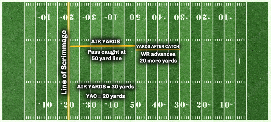
Air yards on a given play are defined as the yardage distance the ball travels in air, from the line of scrimmage, to the point the receiver catches or does not catch the ball (Congelio, 2023). Air yard distance is tracked in yards from the line of scrimmage, not the true distance the ball travels in air (Hermsmeyer, 2018). Air yards are depicted visually in Figure 1. Air yards involve targeted yards—whether or not the pass was completed—and do not include yards after the catch. For a given play in which there is a completed pass, the passing or receiving yards on that play is equal to the sum of the air yards and yards after the catch on that play. Receiving air yards over the course of a game are calculated as the sum of air yards in that game for all passes targeting the player. Receiving air yards thus represent an important index of a wide receiver’s opportunity, volume, or usage (Hermsmeyer, 2018). Hereafter, I refer to receiving air yards as simply “air yards”.
Fantasy managers often must decide whether to trust a player’s previous production or to consider opportunity metrics such as air yards. Understanding which better predicts future fantasy performance can improve weekly start/sit decisions and waiver pickups. One of the goals in fantasy football is to predict which players will do well before they “blow up” and have a big game. Relying on receiving yards, touchdowns, and fantasy points may not be the optimal prognostic indicator of future performance. Although analyzing a wide receiver’s receiving yards or fantasy points tells us about the player’s outcome, it does not indicate how they arrived at that outcome—i.e., how the team used the player, not just what the they caught. It is possible, for instance, that players who get air yards (even if they do not always catch the passes) are more likely to score fantasy points next week than those who just had a good box score (i.e., many receiving yards) last week. Moreover, among underperforming players, considering their air yards may be useful for identifying the ones who are more likely to bounce back in subsequent weeks due to regression to the mean.
Figure 1: Visual Representation of Air Yards. From Congelio (2023).
However, it is not known whether previous performance or opportunity is a stronger predictor of future performance.
4.1 The Present Study
In the present study, I examined whether previous performance or previous opportunity is a stronger predictor of future performance among wide receivers. For the predictors, I operationalized a wide receiver’s performance using their receiving yards, obtained from the nflreadr package (Ho & Carl, 2024). I operationalized a wide receiver’s opportunity using their air yards, obtained from the nflreadr package (Ho & Carl, 2024). For the criterion, I examined wide receivers’ fantasy points in the subsequent game, calculated by Petersen (2025) using the ffanalytics package (Andersen, Petersen, & Tungate, 2025). Thus, I examined the wide receiver’s fantasy points and air yards in a given week in predicting their fantasy points in the subsequent week. Although fantasy points are the ultimate outcome, I examined air yards (opportunity) and receiving yards (performance) as a predictor to isolate the predictive utility of yardage-related receiving opportunity relative to yardage-related receiving production. To my knowledge, this is the first study to examine whether previous performance or opportunity is a stronger predictor of future fantasy performance.
I hypothesized that, due to natural variability from week-to-week that, in part, reflects randomness and is consistent with the statistical principle of regression to the mean, opportunity would be a stronger influence of subsequent performance than previous performance. If the hypothesis is true, I predict that air yards will be a stronger predictor, compared to actual receiving yards, in predicting future fantasy points. Testing this possibility is important for determining what factors may be used to best identify players who, despite not gaining many receiving yards in a given week, may do well in future weeks.
5 Method
To test the hypothesis, I examined whether a wide receiver’s air yards in a given week was a better predictor than their actual receiving yards of the player’s fantasy points the following week.
5.1 Data
Below, I load the data file used for this post. The data file includes weekly player statistics, including air yards, receiving yards, and fantasy points. I obtained the data file from the Open Science Framework repository for the textbook, “Fantasy Football Analytics: Statistics, Prediction, and Empiricism Using R” (Petersen, 2025).
Second, to prepare the data for analysis, I created a lagged variable for fantasy points so that fantasy points in a subsequent year (e.g., 2024) are in the same row as player performance from the prior year (e.g., 2023). Creation of a lagged variable allowed using previous performance to predict future fantasy points.
The original data set includes only those rows for weeks in which a given player played. For instance, if a player played weeks 9 and 11 but missed week 10 due to injury, they would have rows for only week 9 and 11. However, this is a problem if we were to lag a variable (fantasy points) up a row because, in this instance, it would be lagging the variable two weeks (from week 11 to week 9), rather than one week. To ensure that the lagged variable lags only 1 week (and not more weeks), I added missing rows for the missing weeks for given player-season combinations, to ensure each player-season combination had all 18 weeks represented.
Then, I created the lagged variable for fantasy points. I lagged fantasy points within season, so week 1 data did not get lagged to the final week of the prior season.
The lagged variable of fantasy points has fewer observations than the original fantasy points variable because, as mentioned earlier, I lagged data within seasons; consequently, week 1 data were not lagged to the prior season and thus were not retained in the lagged variable.
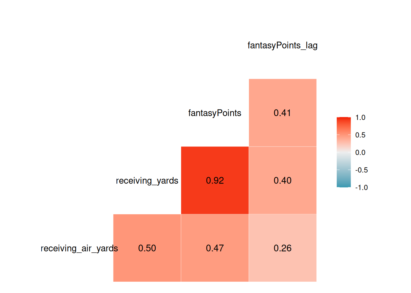
Here is a correlation matrix of the relevant variables:
Code
petersenlab::cor.table(analysisData[,modelVars])
Figure 2 depicts a correlation matrix plot of the relevant variables.
I used multiple regression to test the hypothesis. Specifically, I compared the standardized regression coefficients for the two predictors of interest: air yards versus receiving yards.
6 Results
6.1 Main Analyses
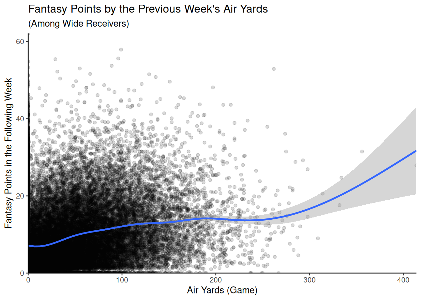
Figure 3 depicts the association between air yards in a given game and their fantasy points the following week among wide receivers.
Code
ggplot2::ggplot(data = analysisData,aes(x = receiving_air_yards,y = fantasyPoints_lag)) +geom_point(alpha =0.15) +geom_smooth() +coord_cartesian(xlim =c(0,NA),ylim =c(0,NA),expand =FALSE) +labs(x ="Air Yards (Game)",y ="Fantasy Points in the Following Week",title ="Fantasy Points by the Previous Week's Air Yards",subtitle ="(Among Wide Receivers)" ) +theme_classic()
Figure 3: Association Between Air Yards and the Player’s Fantasy Points in the Following Week.
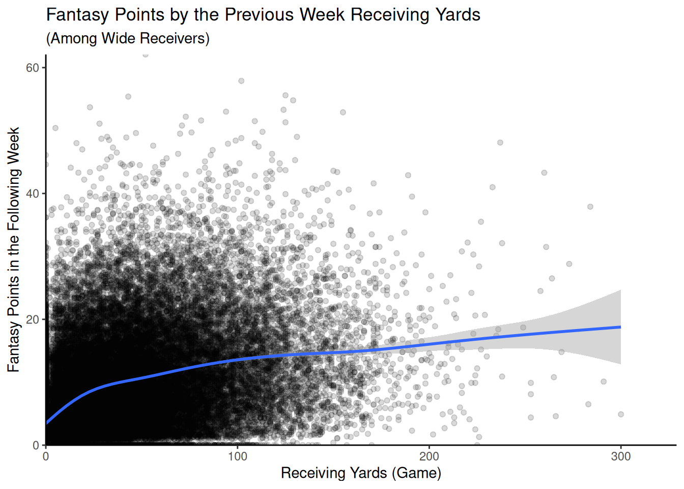
Figure 4 depicts the association between receiving yards in a given game and their fantasy points the following week among wide receivers.
Code
ggplot2::ggplot(data = analysisData,aes(x = receiving_yards,y = fantasyPoints_lag)) +geom_point(alpha =0.15) +geom_smooth() +coord_cartesian(xlim =c(0,NA),ylim =c(0,NA),expand =FALSE) +labs(x ="Receiving Yards (Game)",y ="Fantasy Points in the Following Week",title ="Fantasy Points by the Previous Week Receiving Yards",subtitle ="(Among Wide Receivers)" ) +theme_classic()
Figure 4: Association Between Receiving Yards and the Player’s Fantasy Points in the Following Week.
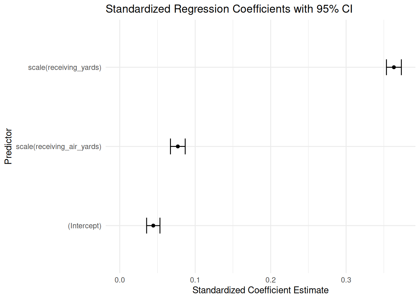
Figure 5: Standardized Regression Coefficients with 95% Confidence Interval.
The standardized regression coefficient for receiving yards was larger than for air yards. As shown in Figure 5, their 95% confidence intervals did not overlap, indicating that the standardized regression coefficient for receiving yards was larger than for air yards. The standardized regression coefficient for air yards in predicting fantasy points was \(\beta = 0.08\). The standardized regression coefficient for receiving yards in predicting fantasy points was \(\beta = 0.36\). Thus, receiving yards had a medium effect size, whereas air yards had a small effect size.
6.2 Sensitivity Analyses
I evaluated assumptions of multiple regression: 1) linear association, 2) homoscedasticity, 3) uncorrelated residuals, and 4) normally distributed residuals. To evaluate the assumption of a linear association between the predictor variables and outcome variable, I examined the shape of the associations of air yards and receiving yards with fantasy points using line graphs. The associations of air yards and receiving yards with fantasy points were mostly linear, as depicted in Figures 3 and 4.
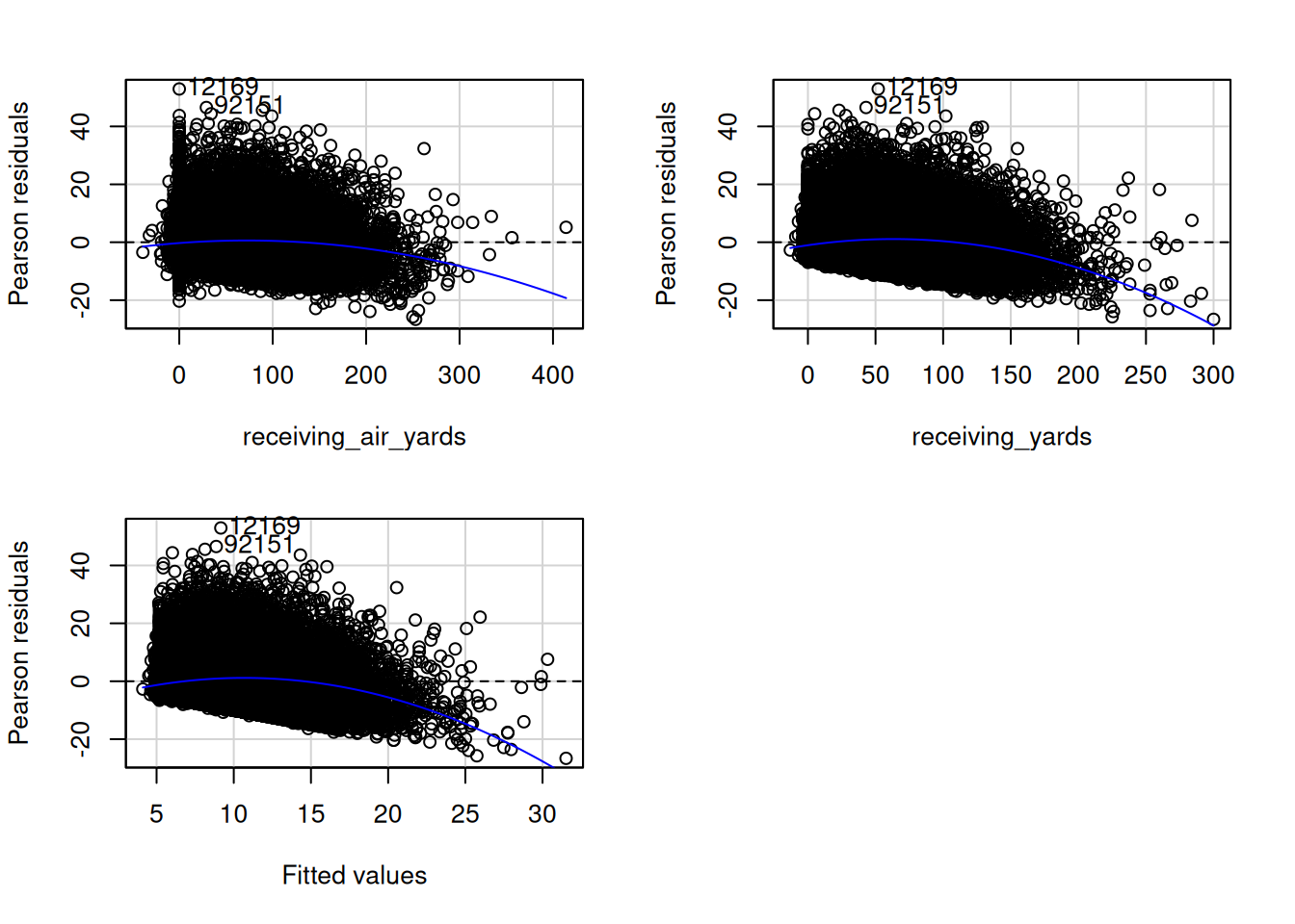
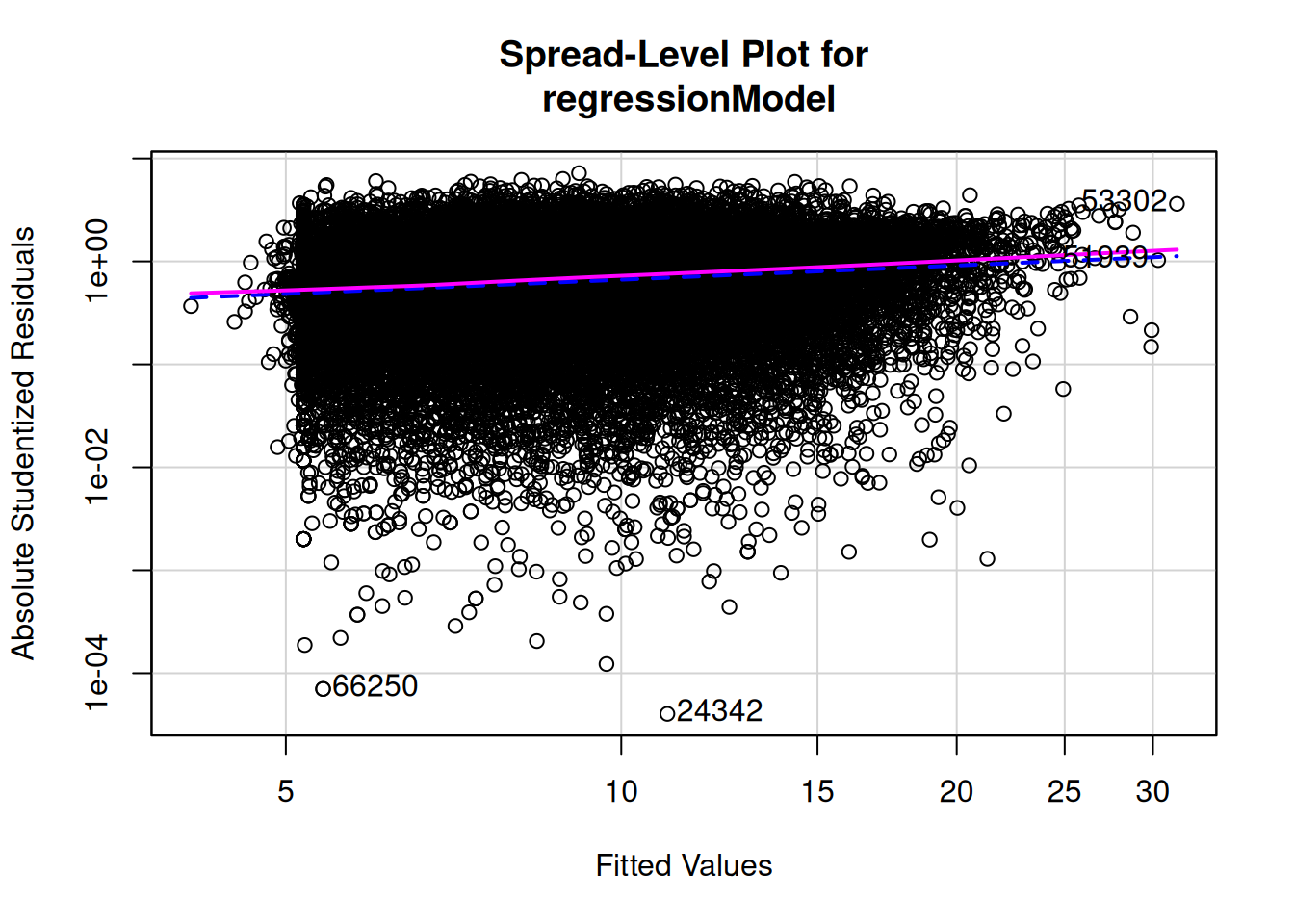
To evaluate the assumption of homoscedasticity, I examined residual and spread-level plots.
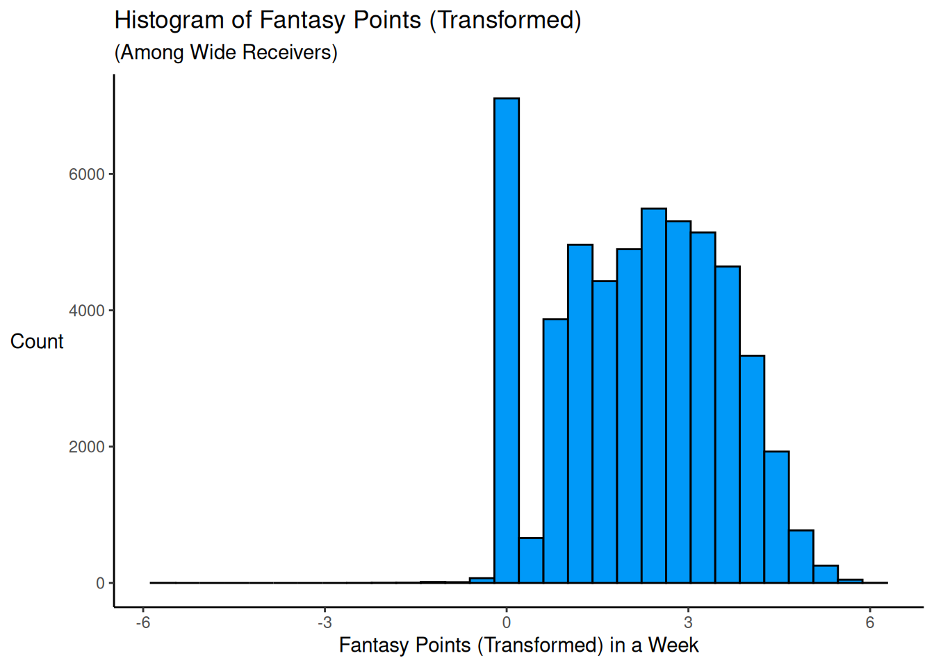
The residuals appeared to increase as a function of the fitted values. To handle this, I conducted a sensitivity analysis by transforming the outcome variable to be more normally distributed. I first identified the best-fitting transformation for (lagged) fantasy points:
Call:
lm(formula = scale(fantasyPoints_lag_transformed) ~ scale(receiving_air_yards) +
    scale(receiving_yards), data = analysisData)

Residuals:
    Min      1Q  Median      3Q     Max
-5.0650 -0.6185 -0.0283  0.5901  4.2404

Coefficients:
                           Estimate Std. Error t value Pr(>|t|)
(Intercept)                0.050609   0.004345   11.65   <2e-16 ***
scale(receiving_air_yards) 0.081937   0.004796   17.08   <2e-16 ***
scale(receiving_yards)     0.379518   0.004848   78.29   <2e-16 ***
---
Signif. codes:  0 '***' 0.001 '**' 0.01 '*' 0.05 '.' 0.1 ' ' 1

Residual standard error: 0.8958 on 42771 degrees of freedom
  (54228 observations deleted due to missingness)
Multiple R-squared:  0.1917,    Adjusted R-squared:  0.1916
F-statistic:  5071 on 2 and 42771 DF,  p-value: < 2.2e-16
The pattern of findings did not differ substantially when transforming the outcome variable to be more normally distributed.
Because the data were nested within players (i.e., longitudinal) and thus violated the assumption of uncorrelated residuals, we also conducted a sensitivity analysis using a mixed model to account for the nested data.
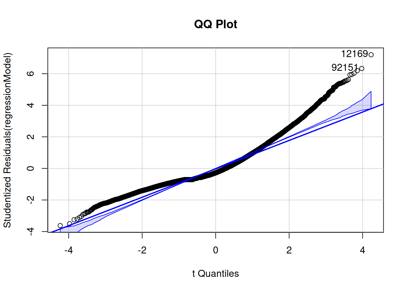
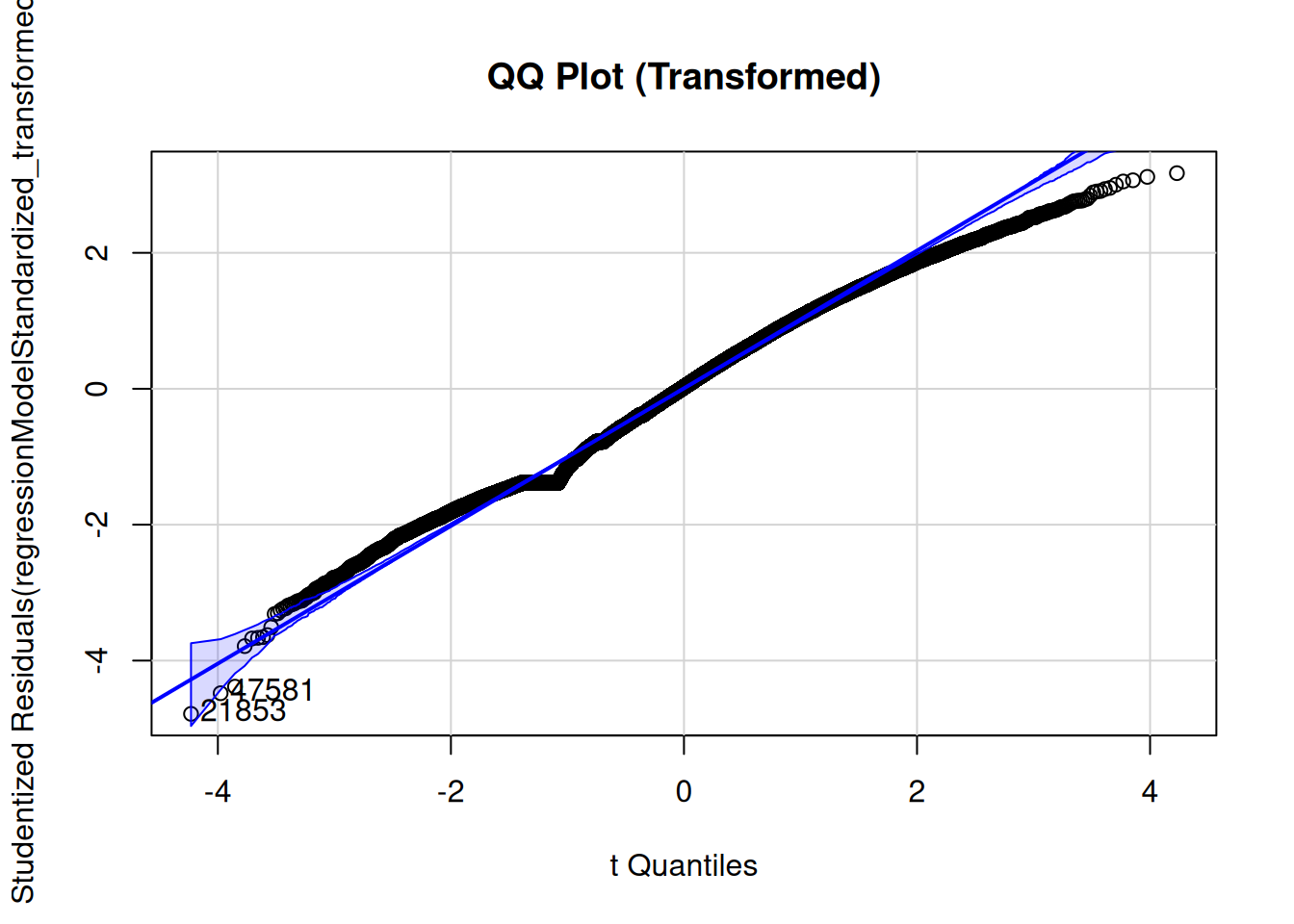
The residuals showed some deviations from normality. However, the residuals from the model with a transformed outcome variable showed some improvements in terms of deviations from normality, as depicted in Figure 11.
In sum, the pattern of findings held after conducting sensitivity analyses to account for potential violations of assumptions of multiple regression.
7 Discussion
In this article, I examined whether previous performance or opportunity is a stronger predictor of future fantasy performance among wide receivers. For the predictors, I operationalized the wide receiver’s performance as their receiving yards. I operationalized a wide receiver’s opportunity as their air yards, an index of the depth of targets the player received. For the criterion of fantasy performance, I examined wide receivers’ fantasy points in the subsequent game. I hypothesized that opportunity would be a stronger influence of subsequent performance than previous performance and that, as a result, air yards will be a stronger predictor, compared to actual receiving yards, in predicting future fantasy points among wide receivers. Contrary to my hypothesis, however, I found that receiving yards was a stronger predictor than air yards in predicting wide receivers’ fantasy points the following week. Receiving yards had a medium effect size; air yards had a small effect size.
Nevertheless, both previous fantasy points and air yards accounted for unique variance in future fantasy points. The findings held when conducting sensitivity analyses, including transforming the outcome variable to be more normally distributed and using a mixed model to account for the longitudinal nature of the data. Thus, findings suggest that, although previous performance is a stronger predictor than previous opportunity in predicting future fantasy performance among wide receivers, both previous performance and opportunity are important predictors of fantasy performance that should be considered. A possible alternative interpretation of the findings is that previous performance reflects other causal processes (such as ability and opportunity) and that previous performance does not influence future performance per se.
7.1 Strengths and Limitations
The study had several strengths. First, I examined data from all seasons since 1999, thus providing strong statistical power to detect differences in the strength of associations. Second, I conducted several sensitivity analyses, providing additional rigor in the methods and additional confidence in the findings.
The study also had limitations. First, air yards and other statistical indexes depend on many factors such as the game script and, in a given game, may not be representative of a player’s role in the offense. Second, a player’s inclusion of a given week in the analysis required the player to play in the given game and the following week. Player availability could depend, in part, due to usage; for instance, receivers who run more routes, receive more targets, and obtain more air/receiving yards could be more likely to miss a subsequent game due to injury and thus could be missing systematically from my analysis. This possibility would be important for future work to consider.
7.2 Conclusion
In conclusion, previous performance is a stronger predictor than previous opportunity in predicting future fantasy performance among wide receivers. However, both previous performance and opportunity are important predictors of fantasy performance and should be considered when predicting wide receiver fantasy performance. Among underperforming players, air yards—as an index of opportunity—may be a useful way of identifying those who may bounce back in subsequent weeks.