Missing Data
1 Preamble
1.1 Load Libraries
1.2 Load Data
The data for this example were simulated:
Code
mydata_long <- read.csv("./data/mydata_long.csv")2 Full Information Maximum Likelihood
For examples using full information maximum likelihood (FIML), see examples of structural equation models here. You can include cases with missingness on predictors by specifying fixed.x = FALSE.
3 Multiple Imputation
3.1 Describe Missing Data
Code
psych::describe(mydata_long)Code
mice::md.pattern(mydata_long, rotate.names = TRUE)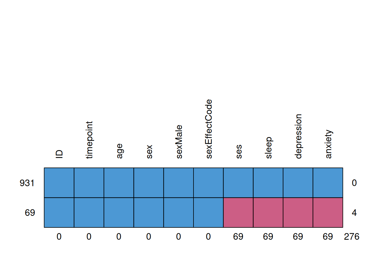
    ID timepoint age sex sexMale sexEffectCode ses sleep depression anxiety
931  1         1   1   1       1             1   1     1          1       1   0
69   1         1   1   1       1             1   0     0          0       0   4
     0         0   0   0       0             0  69    69         69      69 276
3.2 Pre-Imputation Setup
3.2.1 Specify Variables to Impute
Code
varsToImpute <- c("ses","sleep","depression","anxiety")
Y <- varsToImpute
3.2.2 Specify Number of Imputations
Code
numImputations <- 5 # generally use 100 imputations; this example uses 5 for speed3.2.3 Detect Cores
Code
num_cores <- parallelly::availableCores() - 1
num_true_cores <- parallelly::availableCores(logical = FALSE) - 1
3.2.4 Specifying the Imputation Method
You can specify any of various methods to impute each variable. In this case, we use a multilevel imputation (to account for longitudinal data) form of predictive mean matching (2l.pmm from the miceadds package).
Code
imputationMethods <- mice::make.method(mydata_long)
imputationMethods[1:length(imputationMethods)] <- ""
imputationMethods[Y] <- "2l.pmm" # specify the imputation method here; this can differ by outcome variable
imputationMethods
ID timepoint age sex sexMale
"" "" "" "" ""
sexEffectCode ses sleep depression anxiety
"" "2l.pmm" "2l.pmm" "2l.pmm" "2l.pmm" 3.2.5 Specifying the Predictor Matrix
A predictor matrix is a matrix of values, where:
- columns with non-zero values are predictors of the variable specified in the given row
- the diagonal of the predictor matrix should be zero because a variable cannot predict itself
The values are:
- NOT a predictor of the outcome:
0 - cluster variable:
-2 - fixed effect of predictor:
1 - fixed effect and random effect of predictor:
2 - include cluster mean of predictor in addition to fixed effect of predictor:
3 - include cluster mean of predictor in addition to fixed effect and random effect of predictor:
4
Code
predictorMatrix <- mice::make.predictorMatrix(mydata_long)
predictorMatrix[1:nrow(predictorMatrix), 1:ncol(predictorMatrix)] <- 0 # make everything zero by default to manually specify all predictors used for imputation
predictorMatrix[Y, "ID"] <- (-2) # cluster variable
predictorMatrix[Y, "age"] <- 2 # random effect predictor
predictorMatrix[Y, "sexMale"] <- 1 # fixed effect predictor
predictorMatrix[Y, Y] <- 1 # fixed effect predictor; make sure all predictors predict each other

diag(predictorMatrix) <- 0 # don't have a variable predicting itself
predictorMatrix
ID timepoint age sex sexMale sexEffectCode ses sleep depression
ID 0 0 0 0 0 0 0 0 0
timepoint 0 0 0 0 0 0 0 0 0
age 0 0 0 0 0 0 0 0 0
sex 0 0 0 0 0 0 0 0 0
sexMale 0 0 0 0 0 0 0 0 0
sexEffectCode 0 0 0 0 0 0 0 0 0
ses -2 0 2 0 1 0 0 1 1
sleep -2 0 2 0 1 0 1 0 1
depression -2 0 2 0 1 0 1 1 0
anxiety -2 0 2 0 1 0 1 1 1
anxiety
ID 0
timepoint 0
age 0
sex 0
sexMale 0
sexEffectCode 0
ses 1
sleep 1
depression 1
anxiety 03.3 Run Imputation
3.3.1 Sequential Processing
Code
mi_mice <- mice::mice(
  as.data.frame(mydata_long),
  method = imputationMethods,
  predictorMatrix = predictorMatrix,
  m = numImputations,
  maxit = 5, # generally use 100 maximum iterations; this example uses 5 for speed
  seed = 52242)
 iter imp variable
  1   1  ses  sleep  depression  anxiety
  1   2  ses  sleep  depression  anxiety
  1   3  ses  sleep  depression  anxiety
  1   4  ses  sleep  depression  anxiety
  1   5  ses  sleep  depression  anxiety
  2   1  ses  sleep  depression  anxiety
  2   2  ses  sleep  depression  anxiety
  2   3  ses  sleep  depression  anxiety
  2   4  ses  sleep  depression  anxiety
  2   5  ses  sleep  depression  anxiety
  3   1  ses  sleep  depression  anxiety
  3   2  ses  sleep  depression  anxiety
  3   3  ses  sleep  depression  anxiety
  3   4  ses  sleep  depression  anxiety
  3   5  ses  sleep  depression  anxiety
  4   1  ses  sleep  depression  anxiety
  4   2  ses  sleep  depression  anxiety
  4   3  ses  sleep  depression  anxiety
  4   4  ses  sleep  depression  anxiety
  4   5  ses  sleep  depression  anxiety
  5   1  ses  sleep  depression  anxiety
  5   2  ses  sleep  depression  anxiety
  5   3  ses  sleep  depression  anxiety
  5   4  ses  sleep  depression  anxiety
  5   5  ses  sleep  depression  anxiety
3.3.2 Parallel Processing
Code
mi_parallel_mice <- mice::futuremice(
  as.data.frame(mydata_long),
  method = imputationMethods,
  predictorMatrix = predictorMatrix,
  m = numImputations,
  maxit = 5, # generally use 100 maximum iterations; this example uses 5 for speed
  parallelseed = 52242,
  n.core = num_cores,
  packages = "miceadds")
3.4 Imputation Diagnostics
3.4.1 Logged Events
Code
mi_mice$loggedEventsNULL3.4.2 Trace Plots
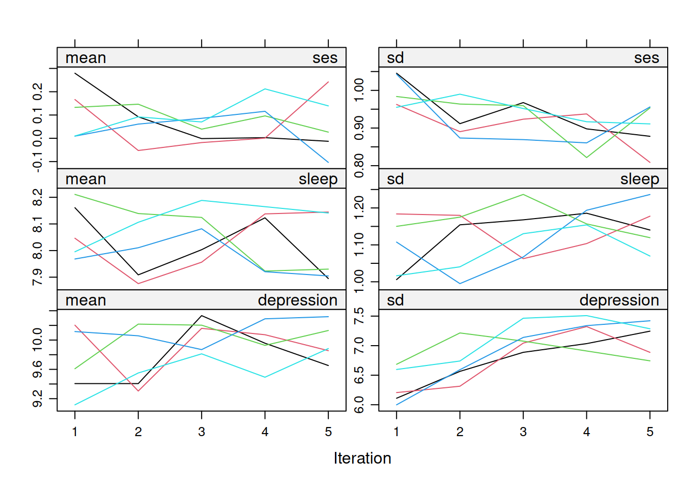
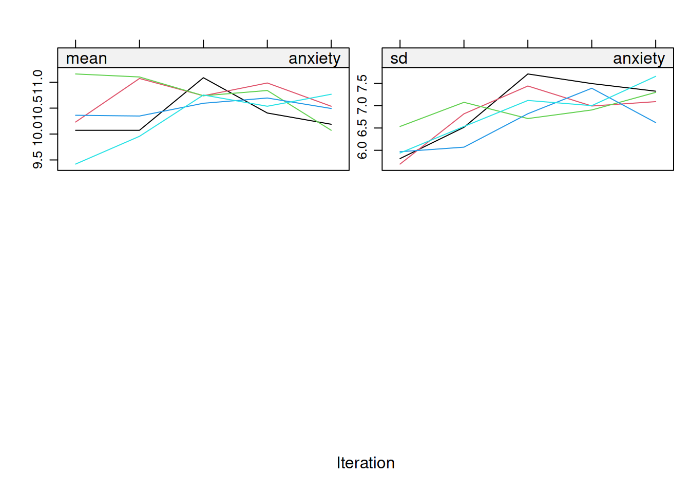
On convergence, the streams of the trace plots should intermingle and be free of any trend (at the later iterations). Convergence is diagnosed when the variance between different sequences is no larger than the variance within each individual sequence.
https://stefvanbuuren.name/fimd/sec-algoptions.html (archived at https://perma.cc/4S54-465R)
3.4.3 Density Plots
Code
mice::densityplot(mi_mice)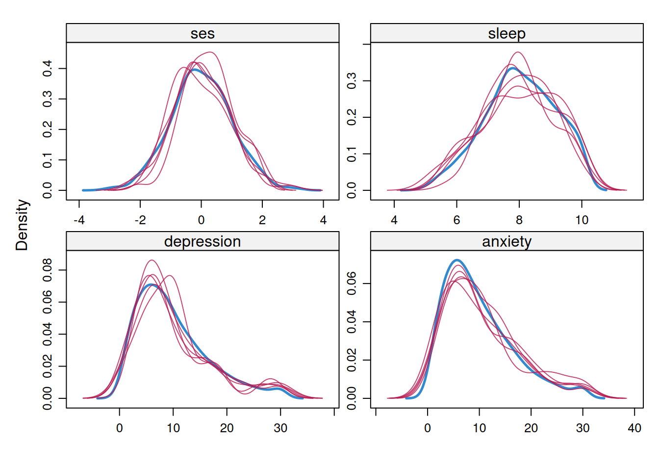
3.4.4 Strip Plots
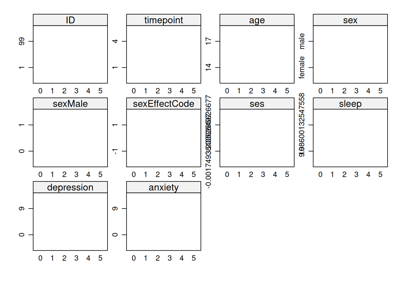
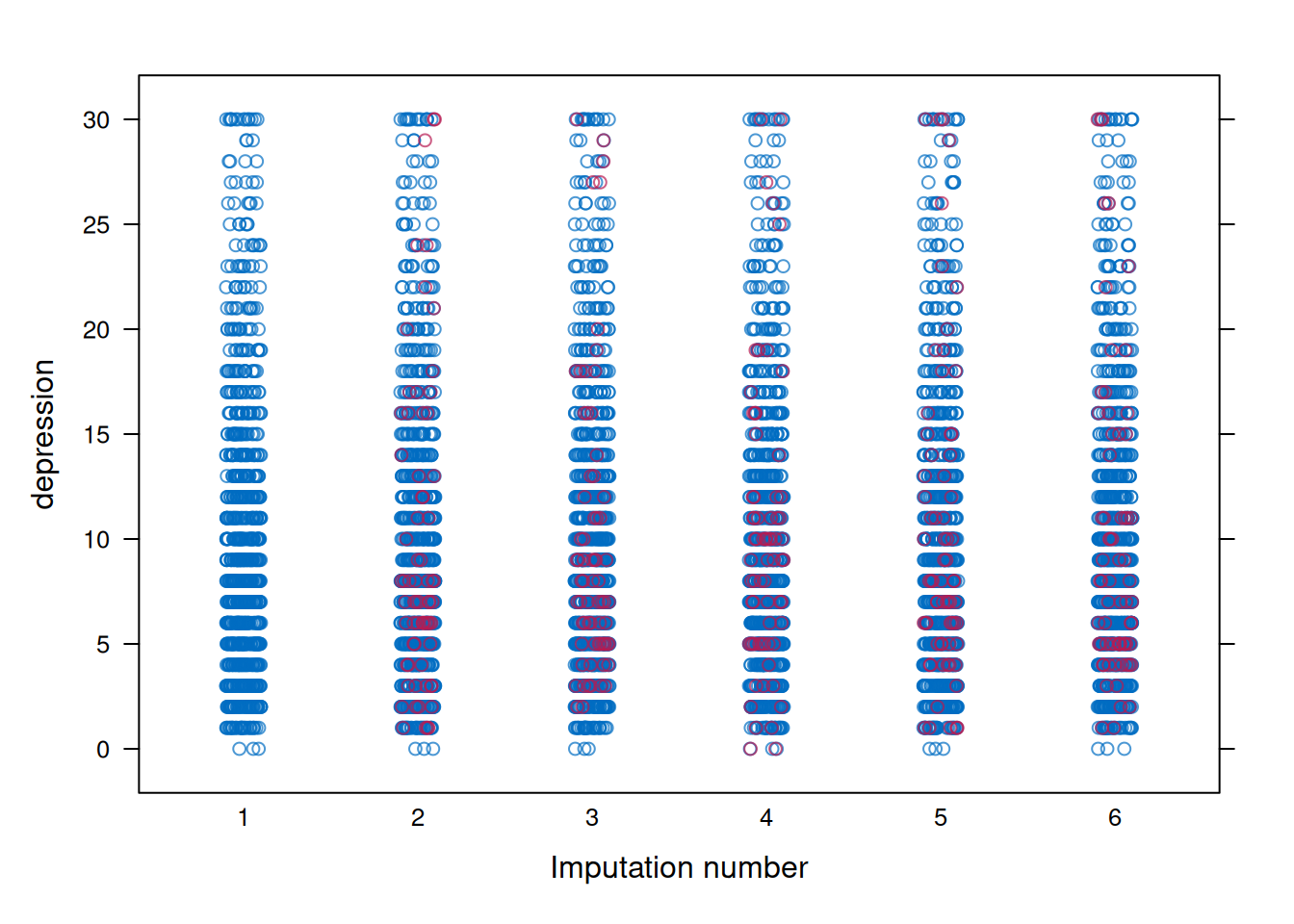
3.5 Post-Processing
3.5.1 Modify/Create New Variables
Code
mi_mice_long <- mice::complete( # return the completed (imputed) data
  mi_mice,
  action = "long",
  include = TRUE)

mi_mice_long <- mi_mice_long |> # long form for mixed-effects modeling
  group_by(ID, .imp) |>
  mutate(
    sexFactor = factor(sex),
    ageCentered = age - min(age, na.rm = TRUE),
    ageCenteredSquared = ageCentered ^ 2,
    ses_personMean = mean(ses, na.rm = TRUE),
    ses_personMeanCentered = ses - ses_personMean,
    sleep_personMean = mean(sleep, na.rm = TRUE),
    sleep_personMeanCentered = sleep - sleep_personMean,
    depression_personMean = mean(depression, na.rm = TRUE),
    depression_personMeanCentered = depression - depression_personMean,
    anxiety_personMean = mean(anxiety, na.rm = TRUE),
    anxiety_personMeanCentered = anxiety - anxiety_personMean,
  ) |>
  ungroup()

mi_mice_wide <- mi_mice_long |> # wide form for structural equation modeling: widen by time
  select(-.id, -age, -ageCentered, -ageCenteredSquared) |> # drop time-varying variables
  tidyr::pivot_wider(
    names_from  = timepoint,
    values_from = c(ses, ses_personMeanCentered, sleep, sleep_personMeanCentered, depression, depression_personMeanCentered, anxiety, anxiety_personMeanCentered)
  )
3.5.2 Convert to mids object
3.6 Fit Models to Multiple Imputed Data
3.6.1 Mixed-Effects Models
3.6.1.1 Fit Model
Code
linearGCM_mice <- with(
  data = mi_mice_long_mids,
  expr = lmerTest::lmer(
    formula = depression ~ sexFactor + ageCentered + sexFactor:ageCentered +
      sleep + sleep:ageCentered + sexFactor:sleep + sexFactor:sleep:ageCentered +
      (1 + ageCentered | ID), # random intercepts and slopes; sex as a fixed-effect predictor of the intercepts and slopes
  )
)
3.6.1.2 Model Summary
Code
linearGCM_micecall :
with.mids(data = mi_mice_long_mids, expr = lmerTest::lmer(formula = depression ~
sexFactor + ageCentered + sexFactor:ageCentered + sleep +
sleep:ageCentered + sexFactor:sleep + sexFactor:sleep:ageCentered +
(1 + ageCentered | ID), ))
call1 :
mice(data = data, m = m, where = where, maxit = 0, remove.collinear = FALSE,
allow.na = TRUE)
nmis :
[1] 0 0 0 0 0 0 69 69 69 69 0 0 0 0 69 0 69 0 69 0 69
analyses :
[[1]]
Linear mixed model fit by REML ['lmerModLmerTest']
Formula: depression ~ sexFactor + ageCentered + sexFactor:ageCentered +
sleep + sleep:ageCentered + sexFactor:sleep + sexFactor:sleep:ageCentered +
(1 + ageCentered | ID)
REML criterion at convergence: 5102.748
Random effects:
Groups Name Std.Dev. Corr
ID (Intercept) 3.789
ageCentered 1.499 0.57
Residual 1.774
Number of obs: 1000, groups: ID, 250
Fixed Effects:
(Intercept) sexFactorfemale
15.35933 1.98820
ageCentered sleep
-0.84863 -0.88422
sexFactorfemale:ageCentered ageCentered:sleep
2.60367 0.01942
sexFactorfemale:sleep sexFactorfemale:ageCentered:sleep
0.04039 -0.12621
[[2]]
Linear mixed model fit by REML ['lmerModLmerTest']
Formula: depression ~ sexFactor + ageCentered + sexFactor:ageCentered +
sleep + sleep:ageCentered + sexFactor:sleep + sexFactor:sleep:ageCentered +
(1 + ageCentered | ID)
REML criterion at convergence: 5099.018
Random effects:
Groups Name Std.Dev. Corr
ID (Intercept) 3.801
ageCentered 1.518 0.55
Residual 1.756
Number of obs: 1000, groups: ID, 250
Fixed Effects:
(Intercept) sexFactorfemale
16.19658 1.07289
ageCentered sleep
-0.63998 -0.99307
sexFactorfemale:ageCentered ageCentered:sleep
2.50714 0.00242
sexFactorfemale:sleep sexFactorfemale:ageCentered:sleep
0.15416 -0.12000
[[3]]
Linear mixed model fit by REML ['lmerModLmerTest']
Formula: depression ~ sexFactor + ageCentered + sexFactor:ageCentered +
sleep + sleep:ageCentered + sexFactor:sleep + sexFactor:sleep:ageCentered +
(1 + ageCentered | ID)
REML criterion at convergence: 5135.067
Random effects:
Groups Name Std.Dev. Corr
ID (Intercept) 3.761
ageCentered 1.497 0.58
Residual 1.827
Number of obs: 1000, groups: ID, 250
Fixed Effects:
(Intercept) sexFactorfemale
16.005936 2.236513
ageCentered sleep
-0.644327 -0.972059
sexFactorfemale:ageCentered ageCentered:sleep
1.985518 0.008007
sexFactorfemale:sleep sexFactorfemale:ageCentered:sleep
0.017228 -0.065530
[[4]]
Linear mixed model fit by REML ['lmerModLmerTest']
Formula: depression ~ sexFactor + ageCentered + sexFactor:ageCentered +
sleep + sleep:ageCentered + sexFactor:sleep + sexFactor:sleep:ageCentered +
(1 + ageCentered | ID)
REML criterion at convergence: 5082.771
Random effects:
Groups Name Std.Dev. Corr
ID (Intercept) 3.799
ageCentered 1.535 0.57
Residual 1.731
Number of obs: 1000, groups: ID, 250
Fixed Effects:
(Intercept) sexFactorfemale
15.84159 1.71636
ageCentered sleep
-1.06624 -0.95303
sexFactorfemale:ageCentered ageCentered:sleep
2.68593 0.06101
sexFactorfemale:sleep sexFactorfemale:ageCentered:sleep
0.08381 -0.15154
[[5]]
Linear mixed model fit by REML ['lmerModLmerTest']
Formula: depression ~ sexFactor + ageCentered + sexFactor:ageCentered +
sleep + sleep:ageCentered + sexFactor:sleep + sexFactor:sleep:ageCentered +
(1 + ageCentered | ID)
REML criterion at convergence: 5114.765
Random effects:
Groups Name Std.Dev. Corr
ID (Intercept) 3.737
ageCentered 1.491 0.63
Residual 1.813
Number of obs: 1000, groups: ID, 250
Fixed Effects:
(Intercept) sexFactorfemale
15.74746 2.14466
ageCentered sleep
-0.47781 -0.93500
sexFactorfemale:ageCentered ageCentered:sleep
2.22335 -0.01803
sexFactorfemale:sleep sexFactorfemale:ageCentered:sleep
0.02546 -0.08941 | Column label | Definition |
|---|---|
m |
Number of imputations |
estimate |
Pooled complete data estimate |
ubar |
Within-imputation variance of estimate
|
b |
Between-imputation variance of estimate
|
t |
Total variance, of estimate
|
dfcom |
Degrees of freedom in complete data |
df |
Residual degrees of freedom for hypothesis testing of \(t\)-statistic |
riv |
Relative increase in variance due to nonresponse |
lambda |
Proportion of total variance due to missingness |
fmi |
Fraction of missing information |
Code
linearGCM_mice_pooled <- mice::pool(linearGCM_mice)

linearGCM_mice_pooled
Class: mipo m = 5
term m estimate ubar b
1 (Intercept) 5 15.83017892 2.256778174 0.0984529972
2 sexFactorfemale 5 1.83172298 4.133072817 0.2188522836
3 ageCentered 5 -0.73539774 0.626591431 0.0515078767
4 sleep 5 -0.94747608 0.033703847 0.0017176927
5 sexFactorfemale:ageCentered 5 2.40112035 1.119580449 0.0844273880
6 ageCentered:sleep 5 0.01456458 0.009444038 0.0008583766
7 sexFactorfemale:sleep 5 0.06420938 0.060787571 0.0031877557
8 sexFactorfemale:ageCentered:sleep 5 -0.11053774 0.016734799 0.0011221435
t dfcom df riv lambda fmi
1 2.37492177 988 593.1339 0.05235056 0.04974631 0.05293437
2 4.39569556 988 507.3527 0.06354176 0.05974543 0.06343016
3 0.68840088 988 319.5232 0.09864395 0.08978700 0.09543133
4 0.03576508 988 524.4955 0.06115715 0.05763251 0.06120550
5 1.22089331 988 353.6699 0.09049181 0.08298257 0.08812468
6 0.01047409 988 282.2755 0.10906901 0.09834285 0.10466416
7 0.06461288 988 511.6980 0.06292909 0.05920347 0.06285920
8 0.01808137 988 402.8435 0.08046539 0.07447290 0.07903391Code
summary(linearGCM_mice_pooled)3.6.2 Structural Equation Models
3.6.2.1 Model Syntax
Code
linearGCM_syntax <- '
  # Intercept and slope
  intercept =~ 1*depression_1 + 1*depression_2 + 1*depression_3 + 1*depression_4
  slope =~ 0*depression_1 + 1*depression_2 + 2*depression_3 + 3*depression_4

  # Regression paths
  intercept ~ sexMale
  slope ~ sexMale

  # Time-varying covariates
  depression_1 ~ sleep_1
  depression_2 ~ sleep_2
  depression_3 ~ sleep_3
  depression_4 ~ sleep_4

  # Constrain observed intercepts to zero
  depression_1 ~ 0
  depression_2 ~ 0
  depression_3 ~ 0
  depression_4 ~ 0

  # Estimate mean of intercept and slope
  intercept ~ 1
  slope ~ 1
'
3.6.2.2 Fit Model
Code
linearGCM_fit_mice <- lavaan.mi::sem.mi(
  linearGCM_syntax,
  data = mi_mice_wide_mids,
  missing = "ML", # FIML
  estimator = "MLR", # Huber-White robust standard errors (for heteroscedasticity and nonnormally distributed residuals)
  meanstructure = TRUE # estimate means/intercepts
)
3.6.2.3 Model Summary
Code
summary(
  linearGCM_fit_mice,
  fit.measures = TRUE,
  standardized = TRUE,
  rsquare = TRUE)
lavaan.mi object fit to 5 imputed data sets using:
- lavaan (0.6-21)
- lavaan.mi (0.1-0)
See class?lavaan.mi help page for available methods.
Convergence information:
The model converged on 5 imputed data sets.
Standard errors were available for all imputations.
Estimator ML
Optimization method NLMINB
Number of model parameters 15
Number of observations 250
Number of missing patterns 1
Model Test User Model:
Standard Scaled
Test statistic 46.920 43.683
Degrees of freedom 19 19
P-value 0.000 0.001
Average scaling correction factor 1.074
Pooling method D4
Pooled statistic "standard"
"yuan.bentler.mplus" correction applied AFTER pooling
Model Test Baseline Model:
Test statistic 1219.809 1049.685
Degrees of freedom 26 26
P-value 0.000 0.000
Scaling correction factor 1.162
User Model versus Baseline Model:
Comparative Fit Index (CFI) 0.977 0.976
Tucker-Lewis Index (TLI) 0.968 0.967
Robust Comparative Fit Index (CFI) 0.977
Robust Tucker-Lewis Index (TLI) 0.968
Loglikelihood and Information Criteria:
Loglikelihood user model (H0) -2477.613 -2477.613
Scaling correction factor 1.228
for the MLR correction
Loglikelihood unrestricted model (H1) -2449.740 -2449.740
Scaling correction factor 1.144
for the MLR correction
Akaike (AIC) 4985.225 4985.225
Bayesian (BIC) 5038.047 5038.047
Sample-size adjusted Bayesian (SABIC) 4990.496 4990.496
Root Mean Square Error of Approximation:
RMSEA 0.077 0.072
90 Percent confidence interval - lower 0.049 0.045
90 Percent confidence interval - upper 0.105 0.099
P-value H_0: RMSEA <= 0.050 0.054 0.087
P-value H_0: RMSEA >= 0.080 0.450 0.334
Robust RMSEA 0.088
90 Percent confidence interval - lower 0.060
90 Percent confidence interval - upper 0.117
P-value H_0: Robust RMSEA <= 0.050 0.015
P-value H_0: Robust RMSEA >= 0.080 0.702
Standardized Root Mean Square Residual:
SRMR 0.082 0.082
Parameter Estimates:
Standard errors Sandwich
Information bread Observed
Observed information based on Hessian
Pooled across imputations Rubin's (1987) rules
Augment within-imputation variance Scale by average RIV
Wald test for pooled parameters t(df) distribution
Pooled t statistics with df >= 1000 are displayed with
df = Inf(inity) to save space. Although the t distribution
with large df closely approximates a standard normal
distribution, exact df for reporting these t tests can be
obtained from parameterEstimates.mi()
Latent Variables:
Estimate Std.Err t-value df P(>|t|) Std.lv
intercept =~
depression_1 1.000 4.038
depression_2 1.000 4.038
depression_3 1.000 4.038
depression_4 1.000 4.038
slope =~
depression_1 0.000 0.000
depression_2 1.000 1.701
depression_3 2.000 3.402
depression_4 3.000 5.104
Std.all
0.935
0.737
0.587
0.472
0.000
0.311
0.495
0.597
Regressions:
Estimate Std.Err t-value df P(>|t|) Std.lv
intercept ~
sexMale -2.314 0.551 -4.203 Inf 0.000 -0.573
slope ~
sexMale -1.539 0.222 -6.925 Inf 0.000 -0.905
depression_1 ~
sleep_1 -0.791 0.131 -6.055 Inf 0.000 -0.791
depression_2 ~
sleep_2 -0.974 0.103 -9.423 804.857 0.000 -0.974
depression_3 ~
sleep_3 -0.990 0.124 -7.982 274.360 0.000 -0.990
depression_4 ~
sleep_4 -0.900 0.179 -5.042 242.711 0.000 -0.900
Std.all
-0.284
-0.449
-0.211
-0.193
-0.157
-0.125
Covariances:
Estimate Std.Err t-value df P(>|t|) Std.lv
.intercept ~~
.slope 3.104 0.521 5.954 782.471 0.000 0.527
Std.all
0.527
Intercepts:
Estimate Std.Err t-value df P(>|t|) Std.lv
.depression_1 0.000 0.000
.depression_2 0.000 0.000
.depression_3 0.000 0.000
.depression_4 0.000 0.000
.intercept 17.487 1.127 15.520 Inf 0.000 4.331
.slope 1.177 0.633 1.859 452.471 0.064 0.692
Std.all
0.000
0.000
0.000
0.000
4.331
0.692
Variances:
Estimate Std.Err t-value df P(>|t|) Std.lv
.depression_1 1.717 0.457 3.757 69.505 0.000 1.717
.depression_2 1.817 0.342 5.316 125.818 0.000 1.817
.depression_3 2.115 0.454 4.659 38.212 0.000 2.115
.depression_4 5.681 1.058 5.369 90.930 0.000 5.681
.intercept 14.984 2.035 7.365 Inf 0.000 0.919
.slope 2.310 0.329 7.020 620.663 0.000 0.798
Std.all
0.092
0.061
0.045
0.078
0.919
0.798
R-Square:
Estimate
depression_1 0.908
depression_2 0.939
depression_3 0.955
depression_4 0.922
intercept 0.081
slope 0.202