Structural Equation Models
For an overview of structural equation modeling, see my chapter on “Structural Equation Modeling” in the following textbook:
Petersen, I. T. (2025). Principles of psychological assessment: With applied examples in R. University of Iowa Libraries. https://isaactpetersen.github.io/Principles-Psychological-Assessment. https://doi.org/10.25820/work.007199
1 Preamble
1.1 Load Libraries
1.2 Load Data
2 Research Questions
- What is the form of adolescents’ depressive symptom trajectories across ages 14 to 17?
- Do the trajectories differ between boys and girls?
- Does how much sleep the adolescent receives predict their depressive symptoms over time?
- Does the association between sleep and depressive symptoms differ between boys and girls?
- What is the association between sleep and depressive symptoms at the within-individual level versus between-individual level?
- Does level of anxiety predict later within-person change in depression (and vice versa)?
- Does within-person change in anxiety predict later within-person change in depression (and vice versa)?
- Do our measures show measurement invariance across time? That is, are our scores able to meaningfully compared on the same metric across time?
3 Pre-Model Computation
Code
mydata_long$sexFactor <- factor(mydata_long$sex)

mydata_long <- mydata_long |>
  group_by(ID) |>
  mutate(
    # Compute person mean and mean-centered variables
    ses_personMean = mean(ses, na.rm = TRUE),
    ses_personMeanCentered = ses - ses_personMean,
    sleep_personMean = mean(sleep, na.rm = TRUE),
    sleep_personMeanCentered = sleep - sleep_personMean,
    depression_personMean = mean(depression, na.rm = TRUE),
    depression_personMeanCentered = depression - depression_personMean,
    anxiety_personMean = mean(anxiety, na.rm = TRUE),
    anxiety_personMeanCentered = anxiety - anxiety_personMean,

    # Compute interaction terms
    sexEffectCodeXses = sexEffectCode * ses,
    sexEffectCodeXsleep = sexEffectCode * sleep,
    sexEffectCodeXdepression = sexEffectCode * depression,
    sexEffectCodeXanxiety = sexEffectCode * anxiety,
    sexEffectCodeXsleep_personMean = sexEffectCode * sleep_personMean,
    sexEffectCodeXsleep_personMeanCentered = sexEffectCode * sleep_personMeanCentered
  ) |>
  ungroup()

# Convert data from long to wide (widen data by timepoint)
mydata_wide <- mydata_long |>
  select(-age) |>
  tidyr::pivot_wider(
    names_from  = timepoint, # widen by timepoint
    values_from = c( # widen time-varying variables
      ses, ses_personMeanCentered, sleep, sleep_personMeanCentered, depression,
      depression_personMeanCentered, anxiety, anxiety_personMeanCentered,
      sexEffectCodeXses, sexEffectCodeXsleep, sexEffectCodeXdepression, sexEffectCodeXanxiety,
      sexEffectCodeXsleep_personMeanCentered)
  )
Variable names for the data in wide form:
Code
names(mydata_wide) [1] "ID"
[2] "sex"
[3] "sexMale"
[4] "sexEffectCode"
[5] "sexFactor"
[6] "ses_personMean"
[7] "sleep_personMean"
[8] "depression_personMean"
[9] "anxiety_personMean"
[10] "sexEffectCodeXsleep_personMean"
[11] "ses_1"
[12] "ses_2"
[13] "ses_3"
[14] "ses_4"
[15] "ses_personMeanCentered_1"
[16] "ses_personMeanCentered_2"
[17] "ses_personMeanCentered_3"
[18] "ses_personMeanCentered_4"
[19] "sleep_1"
[20] "sleep_2"
[21] "sleep_3"
[22] "sleep_4"
[23] "sleep_personMeanCentered_1"
[24] "sleep_personMeanCentered_2"
[25] "sleep_personMeanCentered_3"
[26] "sleep_personMeanCentered_4"
[27] "depression_1"
[28] "depression_2"
[29] "depression_3"
[30] "depression_4"
[31] "depression_personMeanCentered_1"
[32] "depression_personMeanCentered_2"
[33] "depression_personMeanCentered_3"
[34] "depression_personMeanCentered_4"
[35] "anxiety_1"
[36] "anxiety_2"
[37] "anxiety_3"
[38] "anxiety_4"
[39] "anxiety_personMeanCentered_1"
[40] "anxiety_personMeanCentered_2"
[41] "anxiety_personMeanCentered_3"
[42] "anxiety_personMeanCentered_4"
[43] "sexEffectCodeXses_1"
[44] "sexEffectCodeXses_2"
[45] "sexEffectCodeXses_3"
[46] "sexEffectCodeXses_4"
[47] "sexEffectCodeXsleep_1"
[48] "sexEffectCodeXsleep_2"
[49] "sexEffectCodeXsleep_3"
[50] "sexEffectCodeXsleep_4"
[51] "sexEffectCodeXdepression_1"
[52] "sexEffectCodeXdepression_2"
[53] "sexEffectCodeXdepression_3"
[54] "sexEffectCodeXdepression_4"
[55] "sexEffectCodeXanxiety_1"
[56] "sexEffectCodeXanxiety_2"
[57] "sexEffectCodeXanxiety_3"
[58] "sexEffectCodeXanxiety_4"
[59] "sexEffectCodeXsleep_personMeanCentered_1"
[60] "sexEffectCodeXsleep_personMeanCentered_2"
[61] "sexEffectCodeXsleep_personMeanCentered_3"
[62] "sexEffectCodeXsleep_personMeanCentered_4"4 Latent Growth Curve Model
4.1 Linear Growth Curve Model
4.1.1 Model Syntax
In estimating linear latent growth curves of depression symptoms, this model specifies:
- latent intercept and slope factors
- the person’s sex (
sexEffectCode) and the person’s average sleep (sleep_personMean; and their interaction;sexEffectCodeXsleep_personMean) as time-invariant predictors of the latent intercept and slope, and - a person’s deviations from their average sleep (
sleep_personMeanCentered; and in interaction with sex;sexEffectCodeXsleep_personMeanCentered) as time-varying covariates predicting concurrent depression symptoms at each wave.
Code
linearGCM_syntax <- '
  # Intercept and slope
  intercept =~ 1*depression_1 + 1*depression_2 + 1*depression_3 + 1*depression_4
  slope =~ 0*depression_1 + 1*depression_2 + 2*depression_3 + 3*depression_4

  # Regression paths
  intercept ~ sexEffectCode + sleep_personMean + sexEffectCodeXsleep_personMean
  slope ~ sexEffectCode + sleep_personMean + sexEffectCodeXsleep_personMean

  # Time-varying covariates
  depression_1 ~ sleep_personMeanCentered_1 + sexEffectCodeXsleep_personMeanCentered_1
  depression_2 ~ sleep_personMeanCentered_2 + sexEffectCodeXsleep_personMeanCentered_2
  depression_3 ~ sleep_personMeanCentered_3 + sexEffectCodeXsleep_personMeanCentered_3
  depression_4 ~ sleep_personMeanCentered_4 + sexEffectCodeXsleep_personMeanCentered_4

  # Constrain observed intercepts to zero
  depression_1 ~ 0*1
  depression_2 ~ 0*1
  depression_3 ~ 0*1
  depression_4 ~ 0*1

  # Estimate mean of intercept and slope
  intercept ~ 1
  slope ~ 1
'
4.1.2 Fit Model
Specifying fixed.x = FALSE would estimate (i.e., would not consider as fixed) means, variances, and covariances of the observed variables. Doing so would allow missing information in the predictors to be included as part of full information maximum likelihood (FIML). However, this gets challenging to use when including both person mean and person-mean-centered variables (due to linear dependencies). Thus, many of these examples do not specify fixed.x = FALSE.
Code
linearGCM_fit <- lavaan::sem(
  linearGCM_syntax,
  data = mydata_wide,
  missing = "ML", # FIML
  estimator = "MLR", # Huber-White robust standard errors (for heteroscedasticity and nonnormally distributed residuals)
  meanstructure = TRUE) # estimate means/intercepts
4.1.3 Model Summary
Code
summary(
  linearGCM_fit,
  fit.measures = TRUE,
  standardized = TRUE,
  rsquare = TRUE)
lavaan 0.6-21 ended normally after 102 iterations
Estimator ML
Optimization method NLMINB
Number of model parameters 23
Used Total
Number of observations 186 250
Number of missing patterns 1
Model Test User Model:
Standard Scaled
Test Statistic 159.403 206.471
Degrees of freedom 35 35
P-value (Chi-square) 0.000 0.000
Scaling correction factor 0.772
Yuan-Bentler correction (Mplus variant)
Model Test Baseline Model:
Test statistic 2772.555 3085.340
Degrees of freedom 50 50
P-value 0.000 0.000
Scaling correction factor 0.899
User Model versus Baseline Model:
Comparative Fit Index (CFI) 0.954 0.944
Tucker-Lewis Index (TLI) 0.935 0.919
Robust Comparative Fit Index (CFI) 0.944
Robust Tucker-Lewis Index (TLI) 0.920
Loglikelihood and Information Criteria:
Loglikelihood user model (H0) -1686.380 -1686.380
Scaling correction factor 1.117
for the MLR correction
Loglikelihood unrestricted model (H1) NA NA
Scaling correction factor 0.909
for the MLR correction
Akaike (AIC) 3418.761 3418.761
Bayesian (BIC) 3492.953 3492.953
Sample-size adjusted Bayesian (SABIC) 3420.104 3420.104
Root Mean Square Error of Approximation:
RMSEA 0.138 0.162
90 Percent confidence interval - lower 0.117 0.138
90 Percent confidence interval - upper 0.160 0.187
P-value H_0: RMSEA <= 0.050 0.000 0.000
P-value H_0: RMSEA >= 0.080 1.000 1.000
Robust RMSEA 0.143
90 Percent confidence interval - lower 0.125
90 Percent confidence interval - upper 0.162
P-value H_0: Robust RMSEA <= 0.050 0.000
P-value H_0: Robust RMSEA >= 0.080 1.000
Standardized Root Mean Square Residual:
SRMR 0.043 0.043
Parameter Estimates:
Standard errors Sandwich
Information bread Observed
Observed information based on Hessian
Latent Variables:
Estimate Std.Err z-value P(>|z|) Std.lv Std.all
intercept =~
depression_1 1.000 4.094 0.913
depression_2 1.000 4.094 0.727
depression_3 1.000 4.094 0.579
depression_4 1.000 4.094 0.449
slope =~
depression_1 0.000 0.000 0.000
depression_2 1.000 1.770 0.314
depression_3 2.000 3.540 0.501
depression_4 3.000 5.309 0.582
Regressions:
Estimate Std.Err z-value P(>|z|) Std.lv Std.all
intercept ~
sexEffectCode -2.312 2.813 -0.822 0.411 -0.565 -0.556
sleep_personMn -1.440 0.348 -4.136 0.000 -0.352 -0.334
sxEffctCdXsl_M 0.164 0.355 0.461 0.645 0.040 0.318
slope ~
sexEffectCode -2.069 1.100 -1.881 0.060 -1.169 -1.151
sleep_personMn -0.354 0.129 -2.744 0.006 -0.200 -0.190
sxEffctCdXsl_M 0.158 0.132 1.201 0.230 0.089 0.709
depression_1 ~
slp_prsnMnCn_1 -1.535 0.255 -6.008 0.000 -1.535 -0.201
sxEffctCX_MC_1 0.070 0.247 0.284 0.776 0.070 0.009
depression_2 ~
slp_prsnMnCn_2 -0.767 0.255 -3.004 0.003 -0.767 -0.076
sxEffctCX_MC_2 -0.394 0.247 -1.592 0.111 -0.394 -0.039
depression_3 ~
slp_prsnMnCn_3 -0.757 0.221 -3.421 0.001 -0.757 -0.062
sxEffctCX_MC_3 0.137 0.228 0.603 0.547 0.137 0.011
depression_4 ~
slp_prsnMnCn_4 -1.203 0.348 -3.461 0.001 -1.203 -0.085
sxEffctCX_MC_4 0.432 0.358 1.208 0.227 0.432 0.031
Covariances:
Estimate Std.Err z-value P(>|z|) Std.lv Std.all
.intercept ~~
.slope 3.520 0.602 5.844 0.000 0.613 0.613
Intercepts:
Estimate Std.Err z-value P(>|z|) Std.lv Std.all
.depression_1 0.000 0.000 0.000
.depression_2 0.000 0.000 0.000
.depression_3 0.000 0.000 0.000
.depression_4 0.000 0.000 0.000
.intercept 21.149 2.772 7.630 0.000 5.166 5.166
.slope 2.693 1.073 2.509 0.012 1.522 1.522
Variances:
Estimate Std.Err z-value P(>|z|) Std.lv Std.all
.depression_1 2.626 0.689 3.814 0.000 2.626 0.131
.depression_2 2.110 0.331 6.373 0.000 2.110 0.067
.depression_3 1.361 0.498 2.732 0.006 1.361 0.027
.depression_4 8.651 1.642 5.270 0.000 8.651 0.104
.intercept 13.916 2.058 6.761 0.000 0.830 0.830
.slope 2.372 0.411 5.776 0.000 0.757 0.757
R-Square:
Estimate
depression_1 0.869
depression_2 0.933
depression_3 0.973
depression_4 0.896
intercept 0.170
slope 0.2434.1.4 Modification Indices
Code
modificationindices(
  linearGCM_fit,
  sort. = TRUE)
4.1.5 Plots
4.1.5.1 Path Diagram
Code
lavaanPlot::lavaanPlot(
  linearGCM_fit,
  coefs = TRUE,
  #covs = TRUE,
  stand = TRUE)
Path Diagram
To create an interactive path diagram, you can use the following syntax:
Code
lavaangui::plot_lavaan(linearGCM_fit)4.1.5.2 Model-Implied Trajectories
Code
linearGCM_fs <- as.data.frame(lavaan::lavPredict(linearGCM_fit))
linearGCM_caseidx <- lavaan::lavInspect(linearGCM_fit, "case.idx")
linearGCM_fs$ID <- mydata_wide$ID[linearGCM_caseidx]
factorScores_linear <- left_join(
mydata_wide,
linearGCM_fs,
by = "ID")
get_params <- function(fit) {
pe <- parameterEstimates(fit)
get <- function(lhs, rhs, op = NULL) {
if (is.null(op)) {
# automatically detect the operator
# priority: =~, ~1, ~
sub <- pe[pe$lhs == lhs & pe$rhs == rhs, ]
if (nrow(sub) == 0) stop(paste("Parameter not found:", lhs, rhs))
out <- sub$est[1]
} else {
sub <- pe[pe$lhs == lhs & pe$rhs == rhs & pe$op == op, ]
if (nrow(sub) == 0) stop(paste("Parameter not found:", lhs, op, rhs))
out <- sub$est[1]
}
return(out)
}
list(pe = pe, get = get)
}
linearGCM_params <- get_params(linearGCM_fit)
long_linear <- factorScores_linear |>
pivot_longer(
cols = matches("depression_|sleep_personMeanCentered_"),
names_to = c(".value", "time"),
names_pattern = "(.*)_(\\d)"
) |>
mutate(
time = as.numeric(time),
time_num = time - 1,
age = recode_values(time, 1 ~ 14, 2 ~ 15, 3 ~ 16, 4 ~ 17)
)
# Compute individuals' model-implied trajectories
long_linear <- long_linear |>
mutate(
beta_sleep = case_when(
time_num == 0 ~ linearGCM_params$get("depression_1", "sleep_personMeanCentered_1"),
time_num == 1 ~ linearGCM_params$get("depression_2", "sleep_personMeanCentered_2"),
time_num == 2 ~ linearGCM_params$get("depression_3", "sleep_personMeanCentered_3"),
time_num == 3 ~ linearGCM_params$get("depression_4", "sleep_personMeanCentered_4")
),
beta_int = case_when(
time_num == 0 ~ linearGCM_params$get("depression_1", "sexEffectCodeXsleep_personMeanCentered_1"),
time_num == 1 ~ linearGCM_params$get("depression_2", "sexEffectCodeXsleep_personMeanCentered_2"),
time_num == 2 ~ linearGCM_params$get("depression_3", "sexEffectCodeXsleep_personMeanCentered_3"),
time_num == 3 ~ linearGCM_params$get("depression_4", "sexEffectCodeXsleep_personMeanCentered_4")
),
yhat =
intercept +
slope * time_num +
beta_sleep * sleep_personMeanCentered +
beta_int * sexEffectCode * sleep_personMeanCentered
)
sleep_stats <- mydata_long |>
group_by(sexFactor, age) |>
summarize(
mean_sleep = mean(sleep, na.rm = TRUE),
sd_sleep = sd(sleep, na.rm = TRUE),
.groups = "drop"
) %>%
mutate(
time = recode_values(age, 14 ~ 1, 15 ~ 2, 16 ~ 3, 17 ~ 4),
time_num = time - 1
)
newData <- expand.grid(
sexFactor = c("female", "male"),
time_num = 0:3,
sleepFactor = c("low sleep", "average sleep", "high sleep")
) |>
left_join(sleep_stats, by = c("sexFactor", "time_num")) |>
mutate(
sleep = case_when(
sleepFactor == "average sleep" ~ mean_sleep,
sleepFactor == "low sleep" ~ mean_sleep - sd_sleep,
sleepFactor == "high sleep" ~ mean_sleep + sd_sleep
),
sexEffectCode = ifelse(sexFactor == "male", 1, -1)
)
# Compute prototypical trajectories
grand_mean_sleep <- mean(mydata_wide$sleep_personMean, na.rm = TRUE)
newData <- newData |>
mutate(
sleep_personMeanCentered = sleep - grand_mean_sleep
)
newData <- newData |>
mutate(
intercept_hat =
linearGCM_params$get("intercept", "", "~1") +
linearGCM_params$get("intercept", "sexEffectCode", "~") * sexEffectCode +
linearGCM_params$get("intercept", "sleep_personMean", "~") * sleep +
linearGCM_params$get("intercept", "sexEffectCodeXsleep_personMean", "~") * sexEffectCode * sleep,
slope_hat =
linearGCM_params$get("slope", "", "~1") +
linearGCM_params$get("slope", "sexEffectCode", "~") * sexEffectCode +
linearGCM_params$get("slope", "sleep_personMean", "~") * sleep +
linearGCM_params$get("slope", "sexEffectCodeXsleep_personMean", "~") * sexEffectCode * sleep
)
newData <- newData |>
mutate(
beta_sleep = case_when(
time_num == 0 ~ linearGCM_params$get("depression_1", "sleep_personMeanCentered_1"),
time_num == 1 ~ linearGCM_params$get("depression_2", "sleep_personMeanCentered_2"),
time_num == 2 ~ linearGCM_params$get("depression_3", "sleep_personMeanCentered_3"),
time_num == 3 ~ linearGCM_params$get("depression_4", "sleep_personMeanCentered_4")
),
beta_int = case_when(
time_num == 0 ~ linearGCM_params$get("depression_1", "sexEffectCodeXsleep_personMeanCentered_1"),
time_num == 1 ~ linearGCM_params$get("depression_2", "sexEffectCodeXsleep_personMeanCentered_2"),
time_num == 2 ~ linearGCM_params$get("depression_3", "sexEffectCodeXsleep_personMeanCentered_3"),
time_num == 3 ~ linearGCM_params$get("depression_4", "sexEffectCodeXsleep_personMeanCentered_4")
),
yhat =
intercept_hat +
slope_hat * time_num +
beta_sleep * sleep_personMeanCentered +
beta_int * sexEffectCode * sleep_personMeanCentered
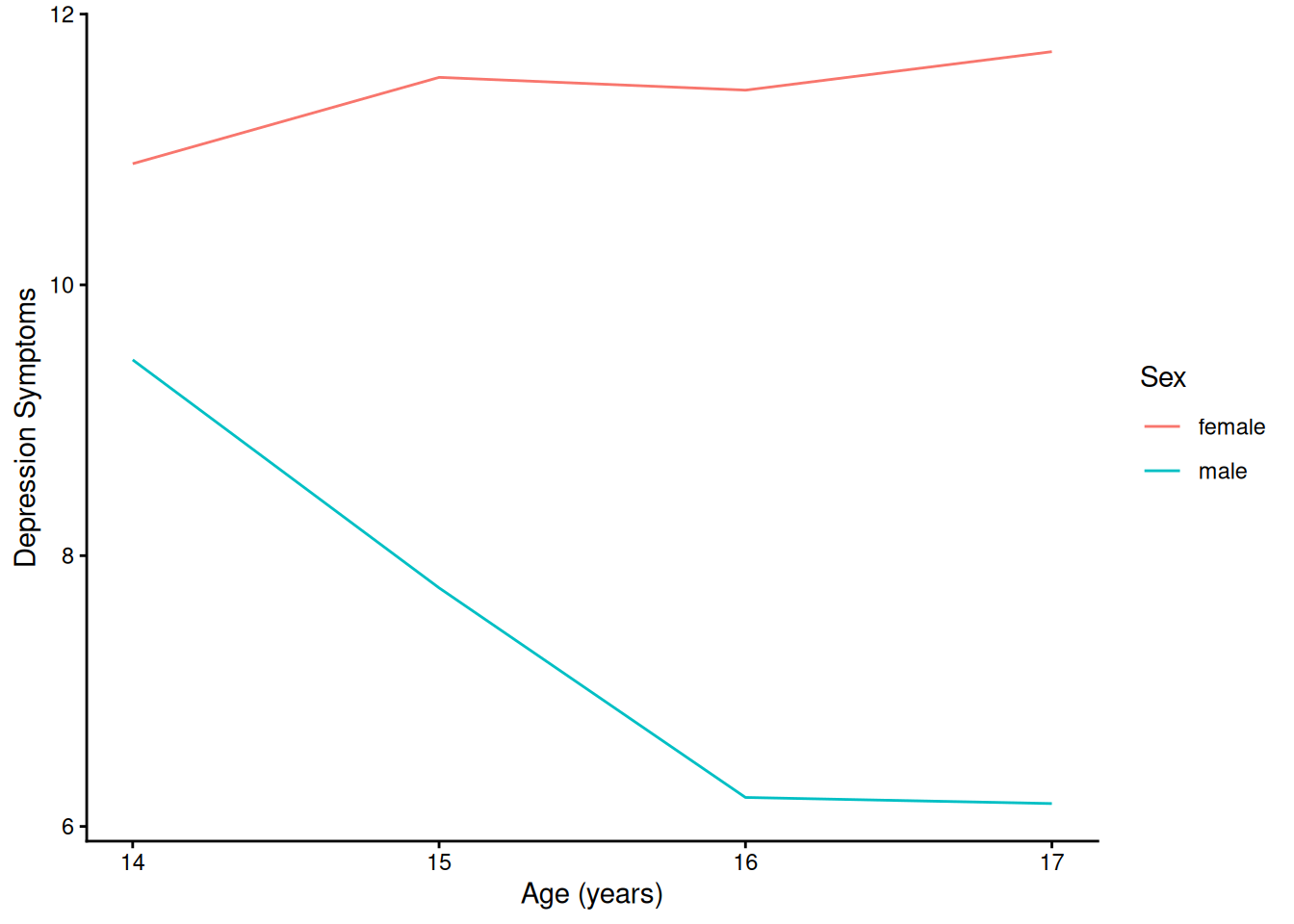
)4.1.5.2.1 Prototypical Growth Curve By Sex
Code
ggplot(
  data = newData |> filter(sleepFactor == "average sleep"),
  mapping = aes(
    x = age,
    y = yhat,
    color = sexFactor)
) +
  geom_smooth( # fit a smoothed line to the model-implied points; use geom_line() to fit a non-smooth line
    method = "lm",
    se = FALSE
  ) +
  labs(
    x = "Age (years)",
    y = "Depression Symptoms",
    color = "Sex"
  ) +
  theme_classic()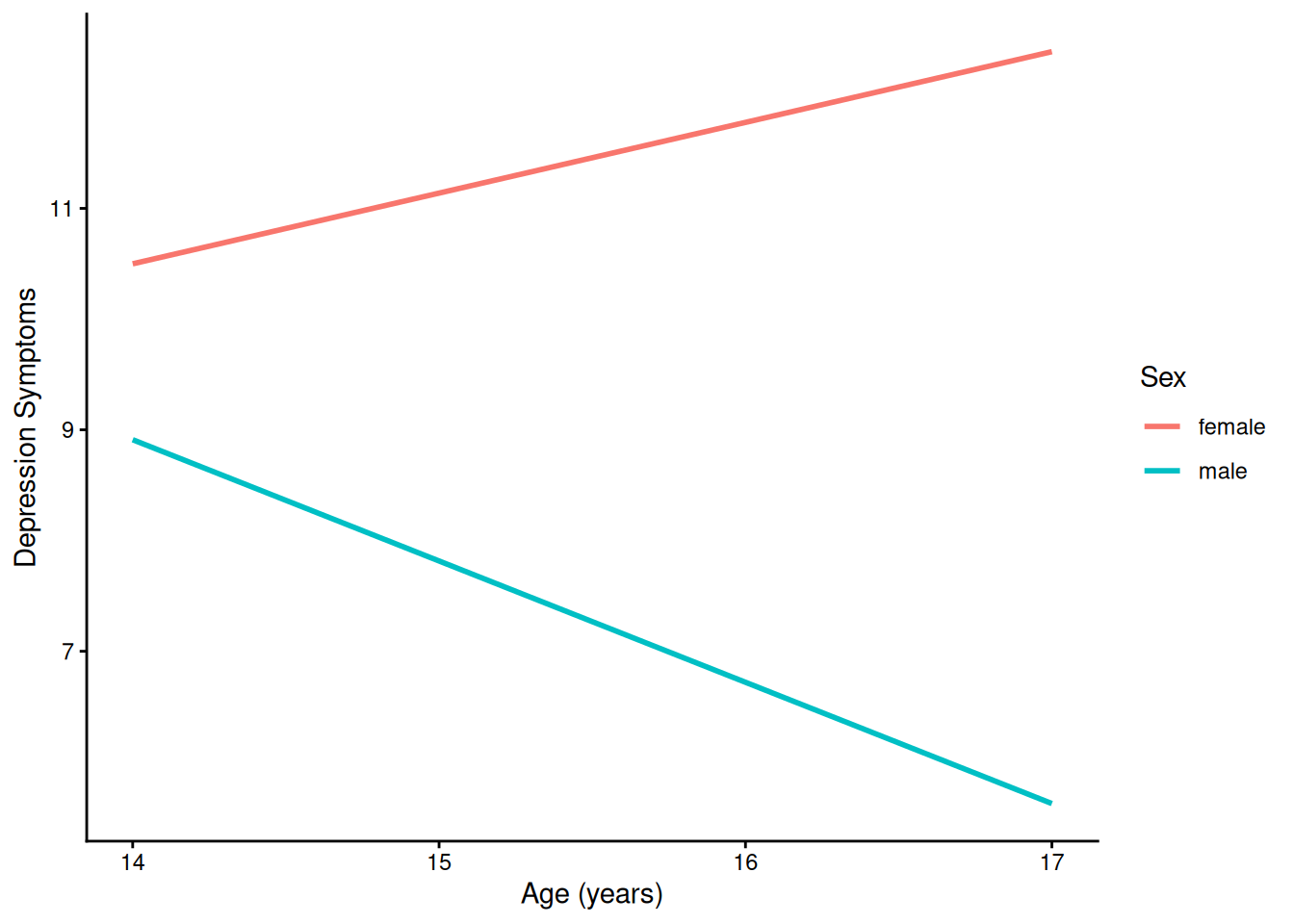
4.1.5.2.2 Individuals’ Growth Curves
Code
ggplot(
  data = long_linear,
  mapping = aes(
    x = age,
    y = yhat,
    group = ID,
    color = sexFactor)
) +
  geom_smooth( # fit a smoothed line to each participant's points; use geom_line() to fit a non-smooth line
    method = "lm",
    se = FALSE,
    linewidth = 0.5
  ) +
  labs(
    x = "Age (years)",
    y = "Depression Symptoms",
    color = "Sex"
  ) +
  theme_classic()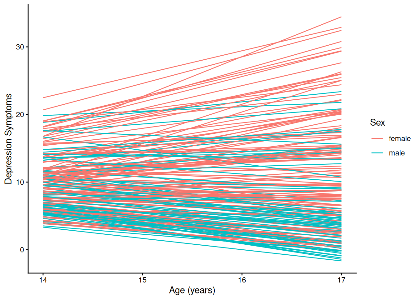
4.1.5.2.3 Individuals’ Trajectories Overlaid with Prototypical Trajectory By Sex
Code
ggplot(
  data = long_linear,
  mapping = aes(
    x = age,
    y = yhat,
    group = ID
  )
) +
  geom_smooth( # fit a smoothed line to each participant's points; use geom_line() to fit a non-smooth line
    method = "lm",
    se = FALSE,
    linewidth = 0.5,
    color = "gray",
    alpha = 0.30
  ) +
  geom_smooth( # fit a smoothed line to the model-implied points; use geom_line() to fit a non-smooth line
    data = newData |> filter(sleepFactor == "average sleep"),
    mapping = aes(
      x = age,
      y = yhat,
      group = sexFactor,
      color = sexFactor
      ),
    method = "lm",
    se = FALSE,
    linewidth = 2
  ) +
  labs(
    x = "Age (years)",
    y = "Depression Symptoms",
    color = "Sex"
  ) +
  theme_classic()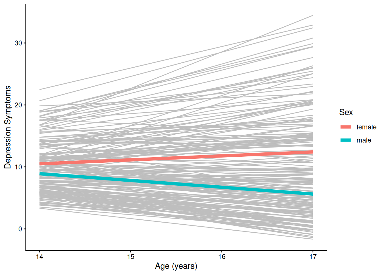
4.1.5.2.4 Prototypical Trajectory By Sex and Sleep
Code
ggplot(
  data = newData |> filter(sleepFactor != "average sleep"),
  mapping = aes(
    x = age,
    y = yhat,
    color = sexFactor,
    linetype = sleepFactor)
) +
  geom_smooth( # fit a smoothed line to the model-implied points; use geom_line() to fit a non-smooth line
    method = "lm",
    se = FALSE
  ) +
  labs(
    x = "Age (years)",
    y = "Depression Symptoms",
    color = "Sex",
    linetype = "Sleep"
  ) +
  guides(
    linetype = guide_legend(
      override.aes = list(color = "black")
    )
  ) +
  theme_classic()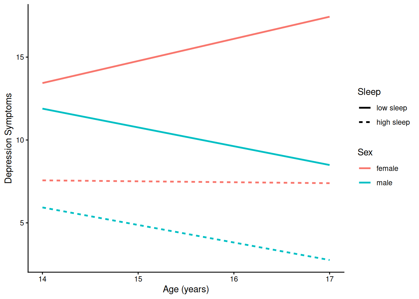
4.2 Quadratic Growth Curve Model
4.2.1 Model Syntax
In estimating quadratic latent growth curves of depression symptoms, this model specifies:
- latent intercept and latent linear and quadratic slope factors
- the person’s sex (
sexEffectCode) and the person’s average sleep (sleep_personMean; and their interaction;sexEffectCodeXsleep_personMean) as time-invariant predictors of the latent intercept and slope, and - a person’s deviations from their average sleep (
sleep_personMeanCentered; and in interaction with sex;sexEffectCodeXsleep_personMeanCentered) as time-varying covariates predicting concurrent depression symptoms at each wave.
Code
quadraticGCM_syntax <- '
  # Intercept and slope
  intercept =~ 1*depression_1 + 1*depression_2 + 1*depression_3 + 1*depression_4
  linear =~ 0*depression_1 + 1*depression_2 + 2*depression_3 + 3*depression_4
  quadratic =~ 0*depression_1 + 1*depression_2 + 4*depression_3 + 9*depression_4

  # Regression paths
  intercept ~ sexEffectCode + sleep_personMean + sexEffectCodeXsleep_personMean
  linear ~ sexEffectCode + sleep_personMean + sexEffectCodeXsleep_personMean
  quadratic ~ sexEffectCode + sleep_personMean + sexEffectCodeXsleep_personMean

  # Time-varying covariates
  depression_1 ~ sleep_personMeanCentered_1 + sexEffectCodeXsleep_personMeanCentered_1
  depression_2 ~ sleep_personMeanCentered_2 + sexEffectCodeXsleep_personMeanCentered_2
  depression_3 ~ sleep_personMeanCentered_3 + sexEffectCodeXsleep_personMeanCentered_3
  depression_4 ~ sleep_personMeanCentered_4 + sexEffectCodeXsleep_personMeanCentered_4

  # Constrain observed intercepts to zero
  depression_1 ~ 0*1
  depression_2 ~ 0*1
  depression_3 ~ 0*1
  depression_4 ~ 0*1

  # Constrain residual variances to be equal (needed to address negative variance)
  depression_1 ~~ vardep*depression_1
  depression_2 ~~ vardep*depression_2
  depression_3 ~~ vardep*depression_3
  depression_4 ~~ vardep*depression_4

  # Estimate mean of intercept and slope
  intercept ~ 1
  linear ~ 1
  quadratic ~ 1
'
4.2.2 Fit Model
Code
quadraticGCM_fit <- lavaan::sem(
  quadraticGCM_syntax,
  data = mydata_wide,
  missing = "ML", # FIML
  estimator = "MLR", # Huber-White robust standard errors (for heteroscedasticity and nonnormally distributed residuals)
  meanstructure = TRUE) # estimate means/intercepts
4.2.3 Model Summary
Code
summary(
  quadraticGCM_fit,
  fit.measures = TRUE,
  standardized = TRUE,
  rsquare = TRUE)
lavaan 0.6-21 ended normally after 142 iterations
Estimator ML
Optimization method NLMINB
Number of model parameters 30
Number of equality constraints 3
Used Total
Number of observations 186 250
Number of missing patterns 1
Model Test User Model:
Standard Scaled
Test Statistic 52.028 74.505
Degrees of freedom 31 31
P-value (Chi-square) 0.010 0.000
Scaling correction factor 0.698
Yuan-Bentler correction (Mplus variant)
Model Test Baseline Model:
Test statistic 2772.555 3085.340
Degrees of freedom 50 50
P-value 0.000 0.000
Scaling correction factor 0.899
User Model versus Baseline Model:
Comparative Fit Index (CFI) 0.992 0.986
Tucker-Lewis Index (TLI) 0.988 0.977
Robust Comparative Fit Index (CFI) 0.987
Robust Tucker-Lewis Index (TLI) 0.980
Loglikelihood and Information Criteria:
Loglikelihood user model (H0) -1632.693 -1632.693
Scaling correction factor 1.036
for the MLR correction
Loglikelihood unrestricted model (H1) NA NA
Scaling correction factor 0.909
for the MLR correction
Akaike (AIC) 3319.386 3319.386
Bayesian (BIC) 3406.481 3406.481
Sample-size adjusted Bayesian (SABIC) 3320.962 3320.962
Root Mean Square Error of Approximation:
RMSEA 0.060 0.087
90 Percent confidence interval - lower 0.029 0.057
90 Percent confidence interval - upper 0.088 0.117
P-value H_0: RMSEA <= 0.050 0.257 0.024
P-value H_0: RMSEA >= 0.080 0.132 0.672
Robust RMSEA 0.072
90 Percent confidence interval - lower 0.050
90 Percent confidence interval - upper 0.094
P-value H_0: Robust RMSEA <= 0.050 0.048
P-value H_0: Robust RMSEA >= 0.080 0.283
Standardized Root Mean Square Residual:
SRMR 0.038 0.038
Parameter Estimates:
Standard errors Sandwich
Information bread Observed
Observed information based on Hessian
Latent Variables:
Estimate Std.Err z-value P(>|z|) Std.lv Std.all
intercept =~
depression_1 1.000 4.101 0.943
depression_2 1.000 4.101 0.717
depression_3 1.000 4.101 0.572
depression_4 1.000 4.101 0.471
linear =~
depression_1 0.000 0.000 0.000
depression_2 1.000 2.628 0.460
depression_3 2.000 5.256 0.733
depression_4 3.000 7.884 0.905
quadratic =~
depression_1 0.000 0.000 0.000
depression_2 1.000 0.646 0.113
depression_3 4.000 2.583 0.360
depression_4 9.000 5.811 0.667
Regressions:
Estimate Std.Err z-value P(>|z|) Std.lv Std.all
intercept ~
sexEffectCode -1.363 2.776 -0.491 0.623 -0.332 -0.327
sleep_personMn -1.415 0.352 -4.021 0.000 -0.345 -0.328
sxEffctCdXsl_M 0.049 0.353 0.139 0.890 0.012 0.095
linear ~
sexEffectCode -5.227 1.880 -2.781 0.005 -1.989 -1.959
sleep_personMn -0.407 0.227 -1.796 0.072 -0.155 -0.147
sxEffctCdXsl_M 0.545 0.227 2.404 0.016 0.207 1.646
quadratic ~
sexEffectCode 1.310 0.560 2.342 0.019 2.029 1.999
sleep_personMn 0.008 0.067 0.121 0.904 0.013 0.012
sxEffctCdXsl_M -0.161 0.067 -2.385 0.017 -0.249 -1.977
depression_1 ~
slp_prsnMnCn_1 -1.336 0.238 -5.621 0.000 -1.336 -0.180
sxEffctCX_MC_1 0.190 0.228 0.835 0.404 0.190 0.026
depression_2 ~
slp_prsnMnCn_2 -0.787 0.266 -2.953 0.003 -0.787 -0.076
sxEffctCX_MC_2 -0.423 0.242 -1.751 0.080 -0.423 -0.041
depression_3 ~
slp_prsnMnCn_3 -0.617 0.198 -3.121 0.002 -0.617 -0.050
sxEffctCX_MC_3 0.286 0.202 1.416 0.157 0.286 0.023
depression_4 ~
slp_prsnMnCn_4 -1.131 0.320 -3.530 0.000 -1.131 -0.084
sxEffctCX_MC_4 0.351 0.330 1.063 0.288 0.351 0.026
Covariances:
Estimate Std.Err z-value P(>|z|) Std.lv Std.all
.intercept ~~
.linear 3.371 1.084 3.109 0.002 0.375 0.375
.quadratic -0.083 0.305 -0.273 0.785 -0.035 -0.035
.linear ~~
.quadratic -1.091 0.356 -3.067 0.002 -0.729 -0.729
Intercepts:
Estimate Std.Err z-value P(>|z|) Std.lv Std.all
.depression_1 0.000 0.000 0.000
.depression_2 0.000 0.000 0.000
.depression_3 0.000 0.000 0.000
.depression_4 0.000 0.000 0.000
.intercept 21.448 2.770 7.743 0.000 5.230 5.230
.linear 1.550 1.882 0.823 0.410 0.590 0.590
.quadratic 0.554 0.559 0.990 0.322 0.857 0.857
Variances:
Estimate Std.Err z-value P(>|z|) Std.lv Std.all
.dprss_1 (vrdp) 1.511 0.238 6.350 0.000 1.511 0.080
.dprss_2 (vrdp) 1.511 0.238 6.350 0.000 1.511 0.046
.dprss_3 (vrdp) 1.511 0.238 6.350 0.000 1.511 0.029
.dprss_4 (vrdp) 1.511 0.238 6.350 0.000 1.511 0.020
.intrcpt 14.179 1.980 7.161 0.000 0.843 0.843
.linear 5.703 1.310 4.352 0.000 0.826 0.826
.quadrtc 0.393 0.111 3.532 0.000 0.942 0.942
R-Square:
Estimate
depression_1 0.920
depression_2 0.954
depression_3 0.971
depression_4 0.980
intercept 0.157
linear 0.174
quadratic 0.0584.2.4 Modification Indices
Code
modificationindices(
  quadraticGCM_fit,
  sort. = TRUE)
4.2.5 Plots
4.2.5.1 Path Diagram
Code
lavaanPlot::lavaanPlot2(
  quadraticGCM_fit,
  stand = TRUE,
  coef_labels = TRUE)
Path Diagram
To create an interactive path diagram, you can use the following syntax:
Code
lavaangui::plot_lavaan(quadraticGCM_fit)4.2.5.2 Model-Implied Trajectories
Code
# Factor scores (latent growth factors) for each individual
quadraticGCM_fs <- as.data.frame(lavaan::lavPredict(quadraticGCM_fit))
quadraticGCM_caseidx <- lavaan::lavInspect(quadraticGCM_fit, "case.idx")
quadraticGCM_fs$ID <- mydata_wide$ID[quadraticGCM_caseidx]

factorScores_quad <- left_join(
  mydata_wide,
  quadraticGCM_fs,
  by = "ID"
)

# Function to extract parameter estimates
quad_params <- get_params(quadraticGCM_fit)

# Compute individuals' model-implied trajectories
long_quad <- factorScores_quad |>
  pivot_longer(
    cols = matches("depression_|sleep_personMeanCentered_"),
    names_to = c(".value", "time"),
    names_pattern = "(.*)_(\\d)"
  ) |>
  mutate(
    time = as.numeric(time),
    time_num = time - 1,
    age = recode_values(time, 1 ~ 14, 2 ~ 15, 3 ~ 16, 4 ~ 17)
  ) |>
  mutate(
    beta_sleep = case_when(
      time_num == 0 ~ quad_params$get("depression_1", "sleep_personMeanCentered_1"),
      time_num == 1 ~ quad_params$get("depression_2", "sleep_personMeanCentered_2"),
      time_num == 2 ~ quad_params$get("depression_3", "sleep_personMeanCentered_3"),
      time_num == 3 ~ quad_params$get("depression_4", "sleep_personMeanCentered_4")
    ),

    beta_int = case_when(
      time_num == 0 ~ quad_params$get("depression_1", "sexEffectCodeXsleep_personMeanCentered_1"),
      time_num == 1 ~ quad_params$get("depression_2", "sexEffectCodeXsleep_personMeanCentered_2"),
      time_num == 2 ~ quad_params$get("depression_3", "sexEffectCodeXsleep_personMeanCentered_3"),
      time_num == 3 ~ quad_params$get("depression_4", "sexEffectCodeXsleep_personMeanCentered_4")
    ),

    yhat =
      intercept +
      linear * time_num +
      quadratic * time_num^2 +
      beta_sleep * sleep_personMeanCentered +
      beta_int * sexEffectCode * sleep_personMeanCentered
  )

# Compute prototypical trajectories
grand_mean_sleep <- mean(mydata_wide$sleep_personMean, na.rm = TRUE)

newData_quad <- expand.grid(
  sexFactor = c("female", "male"),
  time_num = 0:3,
  sleepFactor = c("low sleep", "average sleep", "high sleep")
) |>
  left_join(sleep_stats, by = c("sexFactor", "time_num")) |>
  mutate(
    sleep = case_when(
      sleepFactor == "average sleep" ~ mean_sleep,
      sleepFactor == "low sleep" ~ mean_sleep - sd_sleep,
      sleepFactor == "high sleep" ~ mean_sleep + sd_sleep
    ),
    sexEffectCode = ifelse(sexFactor == "male", 1, -1),
    sleep_personMeanCentered = sleep - grand_mean_sleep
  ) |>
  mutate(
    intercept_hat =
      quad_params$get("intercept", "", "~1") +
      quad_params$get("intercept", "sexEffectCode", "~") * sexEffectCode +
      quad_params$get("intercept", "sleep_personMean", "~") * sleep +
      quad_params$get("intercept", "sexEffectCodeXsleep_personMean", "~") * sexEffectCode * sleep,

    linear_hat =
      quad_params$get("linear", "", "~1") +
      quad_params$get("linear", "sexEffectCode", "~") * sexEffectCode +
      quad_params$get("linear", "sleep_personMean", "~") * sleep +
      quad_params$get("linear", "sexEffectCodeXsleep_personMean", "~") * sexEffectCode * sleep,

    quadratic_hat =
      quad_params$get("quadratic", "", "~1") +
      quad_params$get("quadratic", "sexEffectCode", "~") * sexEffectCode +
      quad_params$get("quadratic", "sleep_personMean", "~") * sleep +
      quad_params$get("quadratic", "sexEffectCodeXsleep_personMean", "~") * sexEffectCode * sleep
  ) |>
  mutate(
    beta_sleep = case_when(
      time_num == 0 ~ quad_params$get("depression_1", "sleep_personMeanCentered_1"),
      time_num == 1 ~ quad_params$get("depression_2", "sleep_personMeanCentered_2"),
      time_num == 2 ~ quad_params$get("depression_3", "sleep_personMeanCentered_3"),
      time_num == 3 ~ quad_params$get("depression_4", "sleep_personMeanCentered_4")
    ),
    beta_int = case_when(
      time_num == 0 ~ quad_params$get("depression_1", "sexEffectCodeXsleep_personMeanCentered_1"),
      time_num == 1 ~ quad_params$get("depression_2", "sexEffectCodeXsleep_personMeanCentered_2"),
      time_num == 2 ~ quad_params$get("depression_3", "sexEffectCodeXsleep_personMeanCentered_3"),
      time_num == 3 ~ quad_params$get("depression_4", "sexEffectCodeXsleep_personMeanCentered_4")
    ),
    yhat =
      intercept_hat +
      linear_hat * time_num +
      quadratic_hat * time_num^2 +
      beta_sleep * sleep_personMeanCentered +
      beta_int * sexEffectCode * sleep_personMeanCentered,
    age = time_num + 14
  )
4.2.5.2.1 Prototypical Growth Curve By Sex
Code
ggplot(
  data = newData_quad |> filter(sleepFactor == "average sleep"),
  mapping = aes(
    x = age,
    y = yhat,
    color = sexFactor)
) +
  geom_smooth( # fit a smoothed line to the model-implied points; use geom_line() to fit a non-smooth line
    method = "lm",
    formula = y ~ x + I(x^2),
    se = FALSE
  ) +
  labs(
    x = "Age (years)",
    y = "Depression Symptoms",
    color = "Sex"
  ) +
  theme_classic()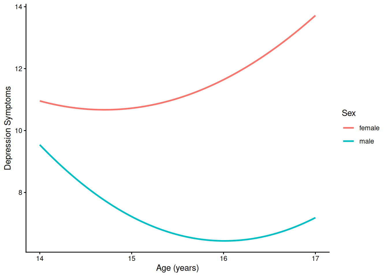
4.2.5.2.2 Individuals’ Growth Curves
Code
ggplot(
  data = long_quad,
  mapping = aes(
    x = age,
    y = yhat,
    group = ID,
    color = sexFactor)
) +
  geom_smooth( # fit a smoothed line to each participant's points; use geom_line() to fit a non-smooth line
    method = "lm",
    formula = y ~ x + I(x^2),
    se = FALSE,
    linewidth = 0.5
  ) +
  labs(
    x = "Age (years)",
    y = "Depression Symptoms",
    color = "Sex"
  ) +
  theme_classic()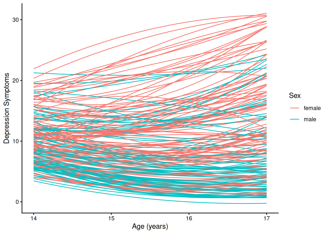
4.2.5.2.3 Individuals’ Trajectories Overlaid with Prototypical Trajectory By Sex
Code
ggplot(
  data = long_quad,
  mapping = aes(
    x = age,
    y = yhat,
    group = ID
  )
) +
  geom_smooth( # fit a smoothed line to each participant's points; use geom_line() to fit a non-smooth line
    method = "lm",
    formula = y ~ x + I(x^2),
    se = FALSE,
    linewidth = 0.5,
    color = "gray",
    alpha = 0.30
  ) +
  geom_smooth( # fit a smoothed line to the model-implied points; use geom_line() to fit a non-smooth line
    data = newData_quad |> filter(sleepFactor == "average sleep"),
    mapping = aes(
      x = age,
      y = yhat,
      group = sexFactor,
      color = sexFactor
      ),
    method = "lm",
    formula = y ~ x + I(x^2),
    se = FALSE,
    linewidth = 2
  ) +
  labs(
    x = "Age (years)",
    y = "Depression Symptoms",
    color = "Sex"
  ) +
  theme_classic()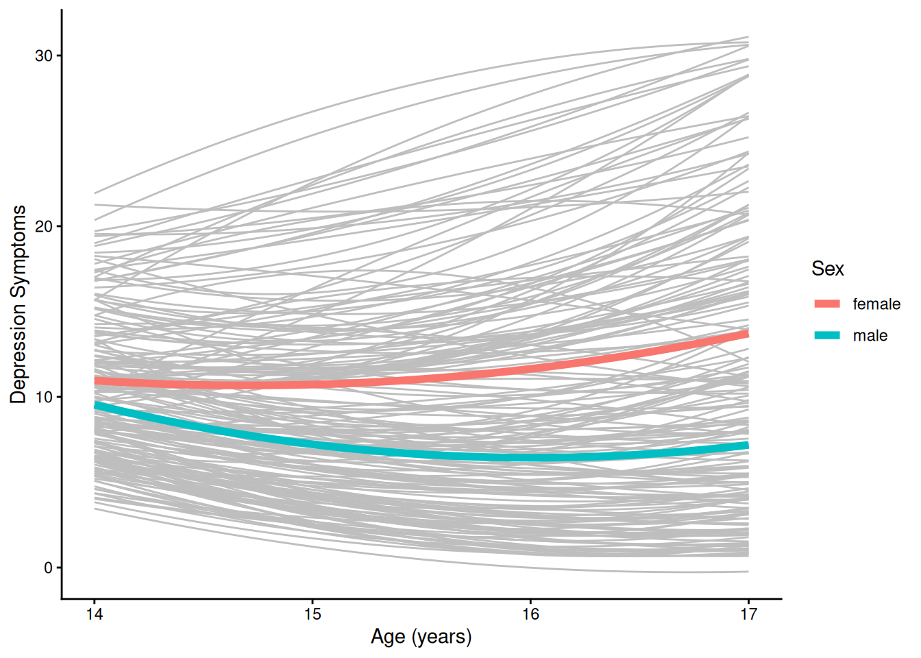
4.2.5.2.4 Prototypical Trajectory By Sex and Sleep
Code
ggplot(
  data = newData_quad |> filter(sleepFactor != "average sleep"),
  mapping = aes(
    x = age,
    y = yhat,
    color = sexFactor,
    linetype = sleepFactor)
) +
  geom_smooth( # fit a smoothed line to the model-implied points; use geom_line() to fit a non-smooth line
    method = "lm",
    formula = y ~ x + I(x^2),
    se = FALSE
  ) +
  labs(
    x = "Age (years)",
    y = "Depression Symptoms",
    color = "Sex",
    linetype = "Sleep"
  ) +
  guides(
    linetype = guide_legend(
      override.aes = list(color = "black")
    )
  ) +
  theme_classic()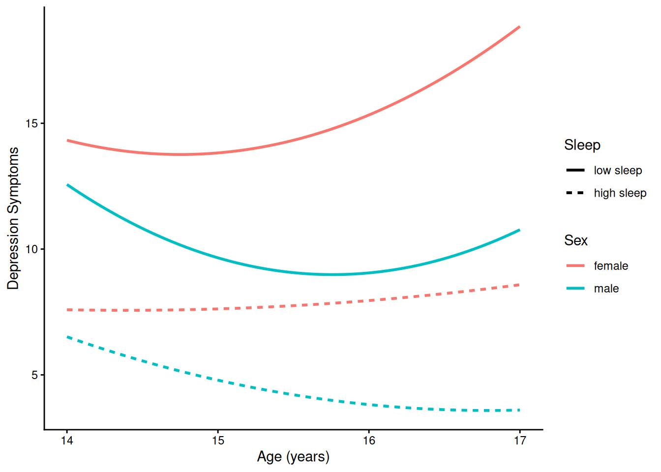
4.3 Latent Basis Growth Curve Model
4.3.1 Model Syntax
In estimating latent basis growth curves of depression symptoms, this model specifies:
- latent intercept and slope factors, with factor loadings for the slope freely estimated at timepoints 2 and 3 to capture nonlinear patterns of change
- the person’s sex (
sexEffectCode) and the person’s average sleep (sleep_personMean; and their interaction;sexEffectCodeXsleep_personMean) as time-invariant predictors of the latent intercept and slope, and - a person’s deviations from their average sleep (
sleep_personMeanCentered; and in interaction with sex;sexEffectCodeXsleep_personMeanCentered) as time-varying covariates predicting concurrent depression symptoms at each wave.
Code
latentBasisGCM_syntax <- '
  # Intercept and slope
  intercept =~ 1*depression_1 + 1*depression_2 + 1*depression_3 + 1*depression_4
  slope =~ 0*depression_1 + a*depression_2 + b*depression_3 + 1*depression_4 # freely estimate the loadings for t2 and t3

  # Regression paths
  intercept ~ sexEffectCode + sleep_personMean + sexEffectCodeXsleep_personMean
  slope ~ sexEffectCode + sleep_personMean + sexEffectCodeXsleep_personMean

  # Time-varying covariates
  depression_1 ~ sleep_personMeanCentered_1 + sexEffectCodeXsleep_personMeanCentered_1
  depression_2 ~ sleep_personMeanCentered_2 + sexEffectCodeXsleep_personMeanCentered_2
  depression_3 ~ sleep_personMeanCentered_3 + sexEffectCodeXsleep_personMeanCentered_3
  depression_4 ~ sleep_personMeanCentered_4 + sexEffectCodeXsleep_personMeanCentered_4

  # Constrain observed intercepts to zero
  depression_1 ~ 0*1
  depression_2 ~ 0*1
  depression_3 ~ 0*1
  depression_4 ~ 0*1

  # Estimate mean of intercept and slope
  intercept ~ 1
  slope ~ 1
'
4.3.2 Fit Model
Code
latentBasisGCM_fit <- lavaan::sem(
  latentBasisGCM_syntax,
  data = mydata_wide,
  missing = "ML", # FIML
  estimator = "MLR", # Huber-White robust standard errors (for heteroscedasticity and nonnormally distributed residuals)
  meanstructure = TRUE) # estimate means/intercepts
A model with negative variances is uninterpretable. We can constrain the variances to be nonnegative using the bounds = "pos.var" argument:
Code
latentBasisGCM_fit <- lavaan::sem(
  latentBasisGCM_syntax,
  data = mydata_wide,
  missing = "ML", # FIML
  estimator = "MLR", # Huber-White robust standard errors (for heteroscedasticity and nonnormally distributed residuals)
  meanstructure = TRUE, # estimate means/intercepts
  bounds = "pos.var") # constrain observed and latent variances to be nonnegative
4.3.3 Model Summary
Code
summary(
  latentBasisGCM_fit,
  fit.measures = TRUE,
  standardized = TRUE,
  rsquare = TRUE)
lavaan 0.6-21 ended normally after 164 iterations
Estimator ML
Optimization method NLMINB
Number of model parameters 25
Row rank of the constraints matrix 6
Used Total
Number of observations 186 250
Number of missing patterns 1
Model Test User Model:
Standard Scaled
Test Statistic 138.748 169.671
Degrees of freedom 33 33
P-value (Chi-square) 0.000 0.000
Scaling correction factor 0.818
Yuan-Bentler correction (Mplus variant)
Model Test Baseline Model:
Test statistic 2772.555 3085.340
Degrees of freedom 50 50
P-value 0.000 0.000
Scaling correction factor 0.899
User Model versus Baseline Model:
Comparative Fit Index (CFI) 0.961 0.955
Tucker-Lewis Index (TLI) 0.941 0.932
Robust Comparative Fit Index (CFI) 0.952
Robust Tucker-Lewis Index (TLI) 0.928
Loglikelihood and Information Criteria:
Loglikelihood user model (H0) -1676.053 -1676.053
Scaling correction factor 1.030
for the MLR correction
Loglikelihood unrestricted model (H1) NA NA
Scaling correction factor 0.909
for the MLR correction
Akaike (AIC) 3402.106 3402.106
Bayesian (BIC) 3482.750 3482.750
Sample-size adjusted Bayesian (SABIC) 3403.566 3403.566
Root Mean Square Error of Approximation:
RMSEA 0.131 0.149
90 Percent confidence interval - lower 0.109 0.125
90 Percent confidence interval - upper 0.154 0.174
P-value H_0: RMSEA <= 0.050 0.000 0.000
P-value H_0: RMSEA >= 0.080 1.000 1.000
Robust RMSEA 0.135
90 Percent confidence interval - lower 0.116
90 Percent confidence interval - upper 0.156
P-value H_0: Robust RMSEA <= 0.050 0.000
P-value H_0: Robust RMSEA >= 0.080 1.000
Standardized Root Mean Square Residual:
SRMR 0.045 0.045
Parameter Estimates:
Standard errors Sandwich
Information bread Observed
Observed information based on Hessian
Latent Variables:
Estimate Std.Err z-value P(>|z|) Std.lv Std.all
intercept =~
depressn_1 1.000 4.211 0.985
depressn_2 1.000 4.211 0.722
depressn_3 1.000 4.211 0.597
depressn_4 1.000 4.211 0.509
slope =~
depressn_1 0.000 0.000 0.000
depressn_2 (a) 0.502 0.043 11.559 0.000 2.411 0.413
depressn_3 (b) 0.885 0.044 20.135 0.000 4.248 0.602
depressn_4 1.000 4.800 0.580
Regressions:
Estimate Std.Err z-value P(>|z|) Std.lv Std.all
intercept ~
sexEffectCode -1.600 2.704 -0.592 0.554 -0.380 -0.374
sleep_personMn -1.381 0.344 -4.016 0.000 -0.328 -0.312
sxEffctCdXsl_M 0.075 0.344 0.218 0.827 0.018 0.142
slope ~
sexEffectCode -6.335 2.613 -2.424 0.015 -1.320 -1.300
sleep_personMn -0.803 0.320 -2.505 0.012 -0.167 -0.159
sxEffctCdXsl_M 0.559 0.312 1.793 0.073 0.116 0.925
depression_1 ~
slp_prsnMnCn_1 -1.367 0.238 -5.758 0.000 -1.367 -0.188
sxEffctCX_MC_1 0.055 0.231 0.238 0.812 0.055 0.008
depression_2 ~
slp_prsnMnCn_2 -0.703 0.241 -2.909 0.004 -0.703 -0.067
sxEffctCX_MC_2 -0.428 0.246 -1.741 0.082 -0.428 -0.041
depression_3 ~
slp_prsnMnCn_3 -0.762 0.216 -3.535 0.000 -0.762 -0.062
sxEffctCX_MC_3 0.276 0.221 1.248 0.212 0.276 0.023
depression_4 ~
slp_prsnMnCn_4 -0.974 0.339 -2.874 0.004 -0.974 -0.076
sxEffctCX_MC_4 0.450 0.342 1.319 0.187 0.450 0.035
Covariances:
Estimate Std.Err z-value P(>|z|) Std.lv Std.all
.intercept ~~
.slope 4.937 1.340 3.683 0.000 0.293 0.293
Intercepts:
Estimate Std.Err z-value P(>|z|) Std.lv Std.all
.depression_1 0.000 0.000 0.000
.depression_2 0.000 0.000 0.000
.depression_3 0.000 0.000 0.000
.depression_4 0.000 0.000 0.000
.intercept 21.135 2.699 7.830 0.000 5.019 5.019
.slope 5.346 2.668 2.004 0.045 1.114 1.114
Variances:
Estimate Std.Err z-value P(>|z|) Std.lv Std.all
.depression_1 0.000 0.000 0.000
.depression_2 2.542 0.317 8.014 0.000 2.542 0.075
.depression_3 0.000 0.000 0.000
.depression_4 11.300 1.594 7.088 0.000 11.300 0.165
.intercept 15.110 1.906 7.926 0.000 0.852 0.852
.slope 18.760 3.087 6.077 0.000 0.814 0.814
R-Square:
Estimate
depression_1 1.000
depression_2 0.925
depression_3 1.000
depression_4 0.835
intercept 0.148
slope 0.1864.3.4 Modification Indices
Code
modificationindices(
  latentBasisGCM_fit,
  sort. = TRUE)
4.3.5 Plots
4.3.5.1 Path Diagram
Code
lavaanPlot::lavaanPlot(
  latentBasisGCM_fit,
  coefs = TRUE,
  #covs = TRUE,
  stand = TRUE)
Path Diagram
To create an interactive path diagram, you can use the following syntax:
Code
lavaangui::plot_lavaan(latentBasisGCM_fit)4.3.5.2 Model-Implied Trajectories
Code
# Factor scores for each individual
latentBasisGCM_fs <- as.data.frame(lavaan::lavPredict(latentBasisGCM_fit))
latentBasisGCM_caseidx <- lavaan::lavInspect(latentBasisGCM_fit, "case.idx")
latentBasisGCM_fs$ID <- mydata_wide$ID[latentBasisGCM_caseidx]

factorScores_lb <- left_join(mydata_wide, latentBasisGCM_fs, by = "ID")

# Function to get parameters (reuse your get_params function)
lb_params <- get_params(latentBasisGCM_fit)

# Get estimated factor loadings
lambda2 <- lb_params$get("slope", "depression_2", "=~") # estimated loading 'a'
lambda3 <- lb_params$get("slope", "depression_3", "=~") # estimated loading 'b'
lambda_vec <- c(0, lambda2, lambda3, 1)

# Compute individuals' model-implied trajectories
long_lb <- factorScores_lb |>
  pivot_longer(
    cols = matches("depression_|sleep_personMeanCentered_"),
    names_to = c(".value", "time"),
    names_pattern = "(.*)_(\\d)"
  ) |>
  mutate(
    time = as.numeric(time),
    time_num = time - 1,
    age = recode_values(time, 1 ~ 14, 2 ~ 15, 3 ~ 16, 4 ~ 17),
    lambda = lambda_vec[time] # latent basis loading for each time
  ) |>
  mutate(
    beta_sleep = case_when(
      time_num == 0 ~ lb_params$get("depression_1", "sleep_personMeanCentered_1"),
      time_num == 1 ~ lb_params$get("depression_2", "sleep_personMeanCentered_2"),
      time_num == 2 ~ lb_params$get("depression_3", "sleep_personMeanCentered_3"),
      time_num == 3 ~ lb_params$get("depression_4", "sleep_personMeanCentered_4")
    ),
    beta_int = case_when(
      time_num == 0 ~ lb_params$get("depression_1", "sexEffectCodeXsleep_personMeanCentered_1"),
      time_num == 1 ~ lb_params$get("depression_2", "sexEffectCodeXsleep_personMeanCentered_2"),
      time_num == 2 ~ lb_params$get("depression_3", "sexEffectCodeXsleep_personMeanCentered_3"),
      time_num == 3 ~ lb_params$get("depression_4", "sexEffectCodeXsleep_personMeanCentered_4")
    ),
    yhat =
      intercept +
      slope * lambda +
      beta_sleep * sleep_personMeanCentered +
      beta_int * sexEffectCode * sleep_personMeanCentered
  )

# Compute prototypical trajectories
grand_mean_sleep <- mean(mydata_wide$sleep_personMean, na.rm = TRUE)

newData_lb <- expand.grid(
  sexFactor = c("female", "male"),
  time_num = 0:3,
  sleepFactor = c("low sleep", "average sleep", "high sleep")
) |>
  left_join(sleep_stats, by = c("sexFactor", "time_num")) |>
  mutate(
    sleep = case_when(
      sleepFactor == "average sleep" ~ mean_sleep,
      sleepFactor == "low sleep" ~ mean_sleep - sd_sleep,
      sleepFactor == "high sleep" ~ mean_sleep + sd_sleep
    ),
    sexEffectCode = ifelse(sexFactor == "male", 1, -1),
    sleep_personMeanCentered = sleep - grand_mean_sleep,
    lambda = lambda_vec[time_num + 1] # latent basis loading for each time
  ) |>
  mutate(
    intercept_hat =
      lb_params$get("intercept", "", "~1") +
      lb_params$get("intercept", "sexEffectCode", "~") * sexEffectCode +
      lb_params$get("intercept", "sleep_personMean", "~") * sleep +
      lb_params$get("intercept", "sexEffectCodeXsleep_personMean", "~") * sexEffectCode * sleep,
    slope_hat =
      lb_params$get("slope", "", "~1") +
      lb_params$get("slope", "sexEffectCode", "~") * sexEffectCode +
      lb_params$get("slope", "sleep_personMean", "~") * sleep +
      lb_params$get("slope", "sexEffectCodeXsleep_personMean", "~") * sexEffectCode * sleep
  ) |>
  mutate(
    beta_sleep = case_when(
      time_num == 0 ~ lb_params$get("depression_1", "sleep_personMeanCentered_1"),
      time_num == 1 ~ lb_params$get("depression_2", "sleep_personMeanCentered_2"),
      time_num == 2 ~ lb_params$get("depression_3", "sleep_personMeanCentered_3"),
      time_num == 3 ~ lb_params$get("depression_4", "sleep_personMeanCentered_4")
    ),
    beta_int = case_when(
      time_num == 0 ~ lb_params$get("depression_1", "sexEffectCodeXsleep_personMeanCentered_1"),
      time_num == 1 ~ lb_params$get("depression_2", "sexEffectCodeXsleep_personMeanCentered_2"),
      time_num == 2 ~ lb_params$get("depression_3", "sexEffectCodeXsleep_personMeanCentered_3"),
      time_num == 3 ~ lb_params$get("depression_4", "sexEffectCodeXsleep_personMeanCentered_4")
    ),
    yhat =
      intercept_hat +
      slope_hat * lambda +
      beta_sleep * sleep_personMeanCentered +
      beta_int * sexEffectCode * sleep_personMeanCentered,
    age = time_num + 14
  )
4.3.5.2.1 Prototypical Growth Curve By Sex
Code
4.3.5.2.2 Individuals’ Growth Curves
Code
ggplot(
  data = long_lb,
  mapping = aes(
    x = age,
    y = yhat,
    group = ID,
    color = sexFactor)
) +
  geom_line(
    alpha = 0.5
  ) +
  labs(
    x = "Age (years)",
    y = "Depression Symptoms",
    color = "Sex"
  ) +
  theme_classic()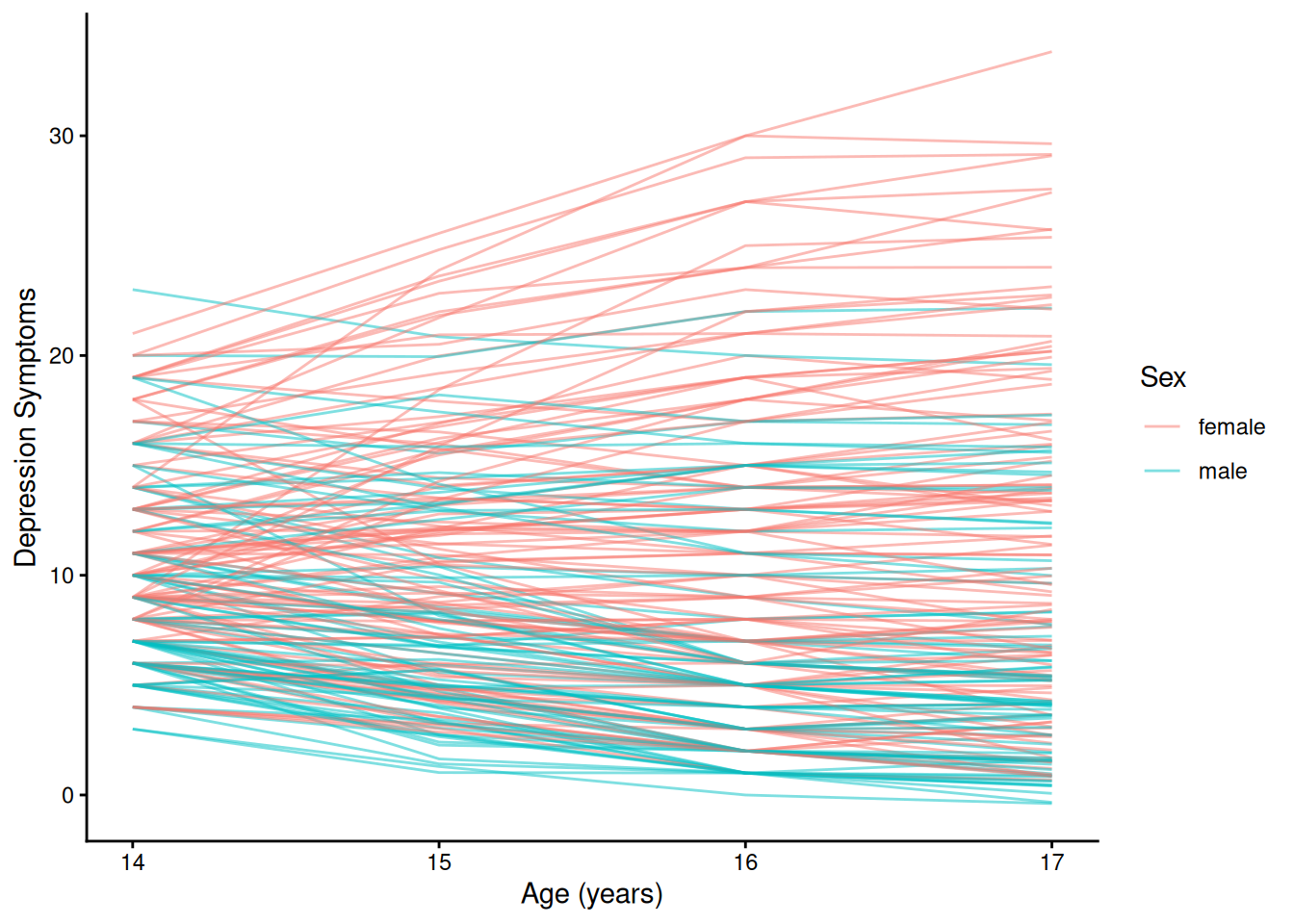
4.3.5.2.3 Individuals’ Trajectories Overlaid with Prototypical Trajectory By Sex
Code
ggplot(
  data = long_lb,
  mapping = aes(
    x = age,
    y = yhat,
    group = ID
  )
) +
  geom_line( # individuals' trajectories
    linewidth = 0.5,
    color = "gray",
    alpha = 0.30
  ) +
  geom_line( # prototypical trajectories
    data = newData_lb |> filter(sleepFactor == "average sleep"),
    mapping = aes(
      x = age,
      y = yhat,
      group = sexFactor,
      color = sexFactor
      ),
    linewidth = 2
  ) +
  labs(
    x = "Age (years)",
    y = "Depression Symptoms",
    color = "Sex"
  ) +
  theme_classic()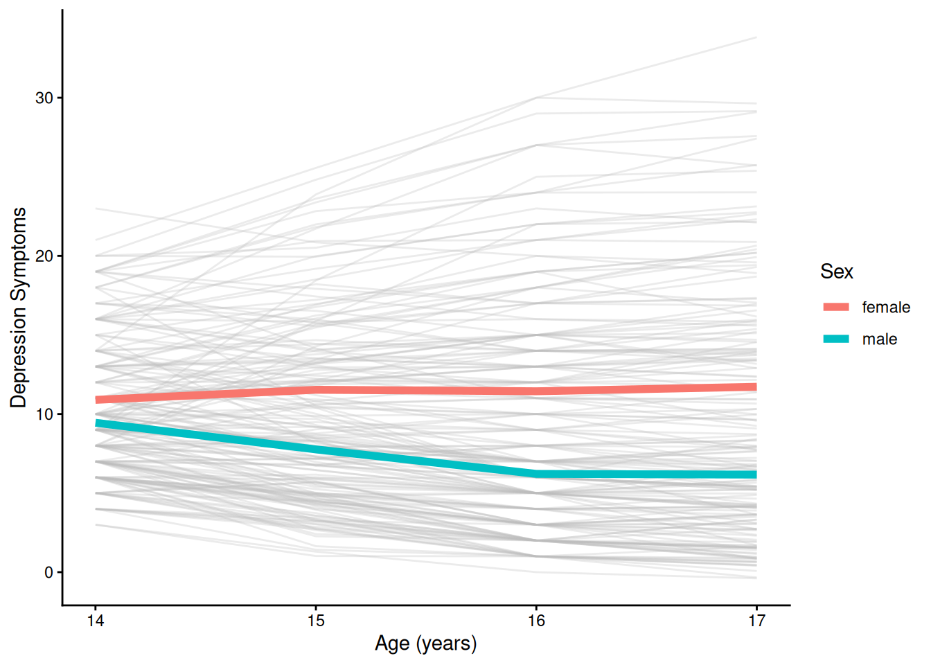
4.3.5.2.4 Prototypical Trajectory By Sex and Sleep
Code
ggplot(
  data = newData_lb |> filter(sleepFactor != "average sleep"),
  mapping = aes(
    x = age,
    y = yhat,
    color = sexFactor,
    linetype = sleepFactor)
) +
  geom_line() +
  labs(
    x = "Age (years)",
    y = "Depression Symptoms",
    color = "Sex",
    linetype = "Sleep"
  ) +
  guides(
    linetype = guide_legend(
      override.aes = list(color = "black")
    )
  ) +
  theme_classic()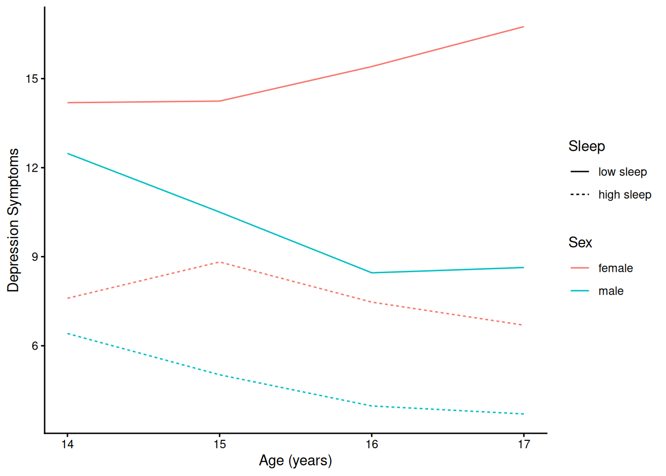
5 Compare Models
6 Latent Change Score Model
6.1 Model Syntax
This model examines reciprocal (i.e., bidirectional), dynamic (i.e., changing) relations between latent change in depression and latent change in anxiety. Each construct is modeled with a latent intercept (constant change factor), a proportional change factor (latent true score predicting its own change), and autoregressive effects of prior change scores. The cross-domain coupling parameters evaluate whether latent change in depression predicts subsequent latent change in anxiety, and vice versa.
Code
bivariateLCSM_syntax <- lcsm::specify_bi_lcsm(
  timepoints = 4,
  var_x = "depression_",
  model_x = list(
    alpha_constant = TRUE, # alpha = intercept (constant change factor)
    beta = TRUE, # beta = proportional change factor (latent true score predicting its change score)
    phi = TRUE), # phi = autoregression of change scores
  var_y = "anxiety_",
  model_y = list(
    alpha_constant = TRUE, # alpha = intercept (constant change factor)
    beta = TRUE, # beta = proportional change factor (latent true score predicting its change score)
    phi = TRUE), # phi = autoregression of change scores
  coupling = list(
    delta_lag_xy = TRUE, # level of x predicting change of y
    delta_lag_yx = TRUE, # level of y predicting change of x
    xi_lag_xy = TRUE,    # change of x predicting change of y
    xi_lag_yx = TRUE),   # change of y predicting change of x
  change_letter_x = "g",
  change_letter_y = "j")

cat(bivariateLCSM_syntax)
# # # # # # # # # # # # # # # # # # # # #
# Specify parameters for construct x ----
# # # # # # # # # # # # # # # # # # # # #
# Specify latent true scores
ldepression_1 =~ 1 * depression_1
ldepression_2 =~ 1 * depression_2
ldepression_3 =~ 1 * depression_3
ldepression_4 =~ 1 * depression_4
# Specify mean of latent true scores
ldepression_1 ~ gamma_ldepression_1 * 1
ldepression_2 ~ 0 * 1
ldepression_3 ~ 0 * 1
ldepression_4 ~ 0 * 1
# Specify variance of latent true scores
ldepression_1 ~~ sigma2_ldepression_1 * ldepression_1
ldepression_2 ~~ 0 * ldepression_2
ldepression_3 ~~ 0 * ldepression_3
ldepression_4 ~~ 0 * ldepression_4
# Specify intercept of obseved scores
depression_1 ~ 0 * 1
depression_2 ~ 0 * 1
depression_3 ~ 0 * 1
depression_4 ~ 0 * 1
# Specify variance of observed scores
depression_1 ~~ sigma2_udepression_ * depression_1
depression_2 ~~ sigma2_udepression_ * depression_2
depression_3 ~~ sigma2_udepression_ * depression_3
depression_4 ~~ sigma2_udepression_ * depression_4
# Specify autoregressions of latent variables
ldepression_2 ~ 1 * ldepression_1
ldepression_3 ~ 1 * ldepression_2
ldepression_4 ~ 1 * ldepression_3
# Specify latent change scores
ddepression_2 =~ 1 * ldepression_2
ddepression_3 =~ 1 * ldepression_3
ddepression_4 =~ 1 * ldepression_4
# Specify latent change scores means
ddepression_2 ~ 0 * 1
ddepression_3 ~ 0 * 1
ddepression_4 ~ 0 * 1
# Specify latent change scores variances
ddepression_2 ~~ 0 * ddepression_2
ddepression_3 ~~ 0 * ddepression_3
ddepression_4 ~~ 0 * ddepression_4
# Specify constant change factor
g2 =~ 1 * ddepression_2 + 1 * ddepression_3 + 1 * ddepression_4
# Specify constant change factor mean
g2 ~ alpha_g2 * 1
# Specify constant change factor variance
g2 ~~ sigma2_g2 * g2
# Specify constant change factor covariance with the initial true score
g2 ~~ sigma_g2ldepression_1 * ldepression_1
# Specify proportional change component
ddepression_2 ~ beta_depression_ * ldepression_1
ddepression_3 ~ beta_depression_ * ldepression_2
ddepression_4 ~ beta_depression_ * ldepression_3
# Specify autoregression of change score
ddepression_3 ~ phi_depression_ * ddepression_2
ddepression_4 ~ phi_depression_ * ddepression_3
# # # # # # # # # # # # # # # # # # # # #
# Specify parameters for construct y ----
# # # # # # # # # # # # # # # # # # # # #
# Specify latent true scores
lanxiety_1 =~ 1 * anxiety_1
lanxiety_2 =~ 1 * anxiety_2
lanxiety_3 =~ 1 * anxiety_3
lanxiety_4 =~ 1 * anxiety_4
# Specify mean of latent true scores
lanxiety_1 ~ gamma_lanxiety_1 * 1
lanxiety_2 ~ 0 * 1
lanxiety_3 ~ 0 * 1
lanxiety_4 ~ 0 * 1
# Specify variance of latent true scores
lanxiety_1 ~~ sigma2_lanxiety_1 * lanxiety_1
lanxiety_2 ~~ 0 * lanxiety_2
lanxiety_3 ~~ 0 * lanxiety_3
lanxiety_4 ~~ 0 * lanxiety_4
# Specify intercept of obseved scores
anxiety_1 ~ 0 * 1
anxiety_2 ~ 0 * 1
anxiety_3 ~ 0 * 1
anxiety_4 ~ 0 * 1
# Specify variance of observed scores
anxiety_1 ~~ sigma2_uanxiety_ * anxiety_1
anxiety_2 ~~ sigma2_uanxiety_ * anxiety_2
anxiety_3 ~~ sigma2_uanxiety_ * anxiety_3
anxiety_4 ~~ sigma2_uanxiety_ * anxiety_4
# Specify autoregressions of latent variables
lanxiety_2 ~ 1 * lanxiety_1
lanxiety_3 ~ 1 * lanxiety_2
lanxiety_4 ~ 1 * lanxiety_3
# Specify latent change scores
danxiety_2 =~ 1 * lanxiety_2
danxiety_3 =~ 1 * lanxiety_3
danxiety_4 =~ 1 * lanxiety_4
# Specify latent change scores means
danxiety_2 ~ 0 * 1
danxiety_3 ~ 0 * 1
danxiety_4 ~ 0 * 1
# Specify latent change scores variances
danxiety_2 ~~ 0 * danxiety_2
danxiety_3 ~~ 0 * danxiety_3
danxiety_4 ~~ 0 * danxiety_4
# Specify constant change factor
j2 =~ 1 * danxiety_2 + 1 * danxiety_3 + 1 * danxiety_4
# Specify constant change factor mean
j2 ~ alpha_j2 * 1
# Specify constant change factor variance
j2 ~~ sigma2_j2 * j2
# Specify constant change factor covariance with the initial true score
j2 ~~ sigma_j2lanxiety_1 * lanxiety_1
# Specify proportional change component
danxiety_2 ~ beta_anxiety_ * lanxiety_1
danxiety_3 ~ beta_anxiety_ * lanxiety_2
danxiety_4 ~ beta_anxiety_ * lanxiety_3
# Specify autoregression of change score
danxiety_3 ~ phi_anxiety_ * danxiety_2
danxiety_4 ~ phi_anxiety_ * danxiety_3
# Specify residual covariances
depression_1 ~~ sigma_su * anxiety_1
depression_2 ~~ sigma_su * anxiety_2
depression_3 ~~ sigma_su * anxiety_3
depression_4 ~~ sigma_su * anxiety_4
# # # # # # # # # # # # # # # # # # # # # # # # # # # # # # # # # # # # # # # # # # # # # # # # # # # # # # # # # # # # # # # #
# Specify covariances betweeen specified change components (alpha) and intercepts (initial latent true scores lx1 and ly1) ----
# # # # # # # # # # # # # # # # # # # # # # # # # # # # # # # # # # # # # # # # # # # # # # # # # # # # # # # # # # # # # # # #
# Specify covariance of intercepts
ldepression_1 ~~ sigma_lanxiety_1ldepression_1 * lanxiety_1
# Specify covariance of constant change and intercept between constructs
lanxiety_1 ~~ sigma_g2lanxiety_1 * g2
# Specify covariance of constant change and intercept between constructs
ldepression_1 ~~ sigma_j2ldepression_1 * j2
# Specify covariance of constant change factors between constructs
g2 ~~ sigma_j2g2 * j2
# # # # # # # # # # # # # # # # # # # # # # # # # # #
# Specify between-construct coupling parameters ----
# # # # # # # # # # # # # # # # # # # # # # # # # # #
# Change score depression_ (t) is determined by true score anxiety_ (t-1)
ddepression_2 ~ delta_lag_depression_anxiety_ * lanxiety_1
ddepression_3 ~ delta_lag_depression_anxiety_ * lanxiety_2
ddepression_4 ~ delta_lag_depression_anxiety_ * lanxiety_3
# Change score anxiety_ (t) is determined by true score depression_ (t-1)
danxiety_2 ~ delta_lag_anxiety_depression_ * ldepression_1
danxiety_3 ~ delta_lag_anxiety_depression_ * ldepression_2
danxiety_4 ~ delta_lag_anxiety_depression_ * ldepression_3
# Change score depression_ (t) is determined by change score anxiety_ (t-1)
ddepression_3 ~ xi_lag_depression_anxiety_ * danxiety_2
ddepression_4 ~ xi_lag_depression_anxiety_ * danxiety_3
# Change score anxiety_ (t) is determined by change score depression_ (t-1)
danxiety_3 ~ xi_lag_anxiety_depression_ * ddepression_2
danxiety_4 ~ xi_lag_anxiety_depression_ * ddepression_3 6.2 Fit Model
Code
bivariateLCSM_fit <- lcsm::fit_bi_lcsm(
  data = mydata_wide,
  var_x = c("depression_1","depression_2","depression_3","depression_4"),
  var_y = c("anxiety_1","anxiety_2","anxiety_3","anxiety_4"),
  model_x = list(
    alpha_constant = TRUE, # alpha = intercept (constant change factor)
    beta = TRUE, # beta = proportional change factor (latent true score predicting its change score)
    phi = TRUE), # phi = autoregression of change scores
  model_y = list(
    alpha_constant = TRUE, # alpha = intercept (constant change factor)
    beta = TRUE, # beta = proportional change factor (latent true score predicting its change score)
    phi = TRUE), # phi = autoregression of change scores
  coupling = list(
    delta_lag_xy = TRUE, # level of x predicting change of y
    delta_lag_yx = TRUE, # level of y predicting change of x
    xi_lag_xy = TRUE,    # change of x predicting change of y
    xi_lag_yx = TRUE),   # change of y predicting change of x
  fixed.x = FALSE # estimate means, variances, and covariances of the observed variables (to include predictors as part of FIML)
  )
6.3 Model Summary
Code
summary(
  bivariateLCSM_fit,
  fit.measures = TRUE,
  standardized = TRUE,
  rsquare = TRUE)
lavaan 0.6-21 ended normally after 913 iterations
Estimator ML
Optimization method NLMINB
Number of model parameters 46
Number of equality constraints 21
Number of observations 250
Number of missing patterns 6
Model Test User Model:
Standard Scaled
Test Statistic 105.533 80.341
Degrees of freedom 19 19
P-value (Chi-square) 0.000 0.000
Scaling correction factor 1.314
Yuan-Bentler correction (Mplus variant)
Model Test Baseline Model:
Test statistic 2762.171 1772.854
Degrees of freedom 28 28
P-value 0.000 0.000
Scaling correction factor 1.558
User Model versus Baseline Model:
Comparative Fit Index (CFI) 0.968 0.965
Tucker-Lewis Index (TLI) 0.953 0.948
Robust Comparative Fit Index (CFI) 0.970
Robust Tucker-Lewis Index (TLI) 0.956
Loglikelihood and Information Criteria:
Loglikelihood user model (H0) -4695.814 -4695.814
Scaling correction factor 0.758
for the MLR correction
Loglikelihood unrestricted model (H1) -4643.048 -4643.048
Scaling correction factor 1.359
for the MLR correction
Akaike (AIC) 9441.628 9441.628
Bayesian (BIC) 9529.664 9529.664
Sample-size adjusted Bayesian (SABIC) 9450.412 9450.412
Root Mean Square Error of Approximation:
RMSEA 0.135 0.114
90 Percent confidence interval - lower 0.110 0.092
90 Percent confidence interval - upper 0.161 0.136
P-value H_0: RMSEA <= 0.050 0.000 0.000
P-value H_0: RMSEA >= 0.080 1.000 0.994
Robust RMSEA 0.138
90 Percent confidence interval - lower 0.106
90 Percent confidence interval - upper 0.172
P-value H_0: Robust RMSEA <= 0.050 0.000
P-value H_0: Robust RMSEA >= 0.080 0.998
Standardized Root Mean Square Residual:
SRMR 0.038 0.038
Parameter Estimates:
Standard errors Sandwich
Information bread Observed
Observed information based on Hessian
Latent Variables:
Estimate Std.Err z-value P(>|z|) Std.lv Std.all
lx1 =~
x1 1.000 4.275 0.950
lx2 =~
x2 1.000 5.600 0.970
lx3 =~
x3 1.000 6.891 0.980
lx4 =~
x4 1.000 8.506 0.987
dx2 =~
lx2 1.000 0.385 0.385
dx3 =~
lx3 1.000 0.240 0.240
dx4 =~
lx4 1.000 0.278 0.278
g2 =~
dx2 1.000 7.049 7.049
dx3 1.000 9.193 9.193
dx4 1.000 6.435 6.435
ly1 =~
y1 1.000 4.157 0.900
ly2 =~
y2 1.000 5.370 0.937
ly3 =~
y3 1.000 6.559 0.956
ly4 =~
y4 1.000 8.308 0.972
dy2 =~
ly2 1.000 0.323 0.323
dy3 =~
ly3 1.000 0.227 0.227
dy4 =~
ly4 1.000 0.267 0.267
j2 =~
dy2 1.000 4.563 4.563
dy3 1.000 5.310 5.310
dy4 1.000 3.566 3.566
Regressions:
Estimate Std.Err z-value P(>|z|) Std.lv Std.all
lx2 ~
lx1 1.000 0.763 0.763
lx3 ~
lx2 1.000 0.813 0.813
lx4 ~
lx3 1.000 0.810 0.810
dx2 ~
lx1 (bt_x) -3.215 1.230 -2.615 0.009 -6.375 -6.375
dx3 ~
lx2 (bt_x) -3.215 1.230 -2.615 0.009 -10.890 -10.890
dx4 ~
lx3 (bt_x) -3.215 1.230 -2.615 0.009 -9.380 -9.380
dx3 ~
dx2 (ph_x) 1.018 1.386 0.735 0.463 1.328 1.328
dx4 ~
dx3 (ph_x) 1.018 1.386 0.735 0.463 0.713 0.713
ly2 ~
ly1 1.000 0.774 0.774
ly3 ~
ly2 1.000 0.819 0.819
ly4 ~
ly3 1.000 0.790 0.790
dy2 ~
ly1 (bt_y) 2.096 1.545 1.357 0.175 5.026 5.026
dy3 ~
ly2 (bt_y) 2.096 1.545 1.357 0.175 7.555 7.555
dy4 ~
ly3 (bt_y) 2.096 1.545 1.357 0.175 6.196 6.196
dy3 ~
dy2 (ph_y) 0.554 1.798 0.308 0.758 0.645 0.645
dy4 ~
dy3 (ph_y) 0.554 1.798 0.308 0.758 0.372 0.372
dx2 ~
ly1 (dlt_lg_x) 3.909 1.537 2.543 0.011 7.537 7.537
dx3 ~
ly2 (dlt_lg_x) 3.909 1.537 2.543 0.011 12.697 12.697
dx4 ~
ly3 (dlt_lg_x) 3.909 1.537 2.543 0.011 10.856 10.856
dy2 ~
lx1 (dlt_lg_y) -1.629 1.189 -1.370 0.171 -4.018 -4.018
dy3 ~
lx2 (dlt_lg_y) -1.629 1.189 -1.370 0.171 -6.124 -6.124
dy4 ~
lx3 (dlt_lg_y) -1.629 1.189 -1.370 0.171 -5.060 -5.060
dx3 ~
dy2 (x_lg_x) -1.514 1.791 -0.845 0.398 -1.587 -1.587
dx4 ~
dy3 (x_lg_x) -1.514 1.791 -0.845 0.398 -0.955 -0.955
dy3 ~
dx2 (x_lg_y) -0.755 1.484 -0.509 0.611 -1.092 -1.092
dy4 ~
dx3 (x_lg_y) -0.755 1.484 -0.509 0.611 -0.562 -0.562
Covariances:
Estimate Std.Err z-value P(>|z|) Std.lv Std.all
lx1 ~~
g2 (sgm_g2lx1) 29.532 11.972 2.467 0.014 0.454 0.454
ly1 ~~
j2 (sgm_j2ly1) -17.998 17.066 -1.055 0.292 -0.547 -0.547
.x1 ~~
.y1 (sgm_) 0.329 0.234 1.405 0.160 0.329 0.116
.x2 ~~
.y2 (sgm_) 0.329 0.234 1.405 0.160 0.329 0.116
.x3 ~~
.y3 (sgm_) 0.329 0.234 1.405 0.160 0.329 0.116
.x4 ~~
.y4 (sgm_) 0.329 0.234 1.405 0.160 0.329 0.116
lx1 ~~
l1 (s_11) 8.558 1.441 5.941 0.000 0.481 0.481
g2 ~~
l1 (sgm_g2ly1) -35.093 16.860 -2.081 0.037 -0.555 -0.555
lx1 ~~
j2 (sgm_j2lx1) 15.378 10.600 1.451 0.147 0.455 0.455
g2 ~~
j2 (s_22) 119.988 131.569 0.912 0.362 0.998 0.998
Intercepts:
Estimate Std.Err z-value P(>|z|) Std.lv Std.all
lx1 (gmm_lx1) 10.145 0.282 35.951 0.000 2.373 2.373
.lx2 0.000 0.000 0.000
.lx3 0.000 0.000 0.000
.lx4 0.000 0.000 0.000
.x1 0.000 0.000 0.000
.x2 0.000 0.000 0.000
.x3 0.000 0.000 0.000
.x4 0.000 0.000 0.000
.dx2 0.000 0.000 0.000
.dx3 0.000 0.000 0.000
.dx4 0.000 0.000 0.000
g2 (alph_g2) -5.497 3.627 -1.516 0.130 -0.362 -0.362
ly1 (gmm_ly1) 9.515 0.288 32.981 0.000 2.289 2.289
.ly2 0.000 0.000 0.000
.ly3 0.000 0.000 0.000
.ly4 0.000 0.000 0.000
.y1 0.000 0.000 0.000
.y2 0.000 0.000 0.000
.y3 0.000 0.000 0.000
.y4 0.000 0.000 0.000
.dy2 0.000 0.000 0.000
.dy3 0.000 0.000 0.000
.dy4 0.000 0.000 0.000
j2 (alph_j2) -3.843 4.529 -0.849 0.396 -0.486 -0.486
Variances:
Estimate Std.Err z-value P(>|z|) Std.lv Std.all
lx1 (sgm2_lx1) 18.279 1.956 9.343 0.000 1.000 1.000
.lx2 0.000 0.000 0.000
.lx3 0.000 0.000 0.000
.lx4 0.000 0.000 0.000
.x1 (sgm2_x) 1.983 0.334 5.945 0.000 1.983 0.098
.x2 (sgm2_x) 1.983 0.334 5.945 0.000 1.983 0.059
.x3 (sgm2_x) 1.983 0.334 5.945 0.000 1.983 0.040
.x4 (sgm2_x) 1.983 0.334 5.945 0.000 1.983 0.027
.dx2 0.000 0.000 0.000
.dx3 0.000 0.000 0.000
.dx4 0.000 0.000 0.000
g2 (sgm2_g2) 230.992 179.739 1.285 0.199 1.000 1.000
ly1 (sgm2_ly1) 17.282 1.602 10.785 0.000 1.000 1.000
.ly2 0.000 0.000 0.000
.ly3 0.000 0.000 0.000
.ly4 0.000 0.000 0.000
.y1 (sgm2_y) 4.030 0.411 9.802 0.000 4.030 0.189
.y2 (sgm2_y) 4.030 0.411 9.802 0.000 4.030 0.123
.y3 (sgm2_y) 4.030 0.411 9.802 0.000 4.030 0.086
.y4 (sgm2_y) 4.030 0.411 9.802 0.000 4.030 0.055
.dy2 0.000 0.000 0.000
.dy3 0.000 0.000 0.000
.dy4 0.000 0.000 0.000
j2 (sgm2_j2) 62.569 91.726 0.682 0.495 1.000 1.000
R-Square:
Estimate
lx2 1.000
lx3 1.000
lx4 1.000
x1 0.902
x2 0.941
x3 0.960
x4 0.973
dx2 1.000
dx3 1.000
dx4 1.000
ly2 1.000
ly3 1.000
ly4 1.000
y1 0.811
y2 0.877
y3 0.914
y4 0.945
dy2 1.000
dy3 1.000
dy4 1.000Code
lcsm::extract_param(bivariateLCSM_fit)6.4 Modification Indices
Code
modificationindices(
  bivariateLCSM_fit,
  sort. = TRUE)
6.5 Plots
6.5.1 Path Diagram
Code
lavaanPlot::lavaanPlot2(
  bivariateLCSM_fit,
  stand = TRUE,
  coef_labels = TRUE)
Path Diagram
To create an interactive path diagram, you can use the following syntax:
Code
lavaangui::plot_lavaan(bivariateLCSM_fit)Code
lcsm::plot_lcsm(
  lavaan_object = bivariateLCSM_fit,
  lcsm = "bivariate",
  lavaan_syntax = bivariateLCSM_syntax,
  edge.label.cex = .9,
  lcsm_colours = TRUE)
6.5.2 Model-Implied Trajectories
To plot model-implied trajectories, see this resource:
https://thechangelab.stanford.edu/tutorials/growth-modeling/latent-change-score-modeling-lavaan/ (archived at https://perma.cc/A2KZ-QPD9)
Code
modelPredictedValues_wide <- as.data.frame(lavPredict(bivariateLCSM_fit, type = "yhat"))

modelPredictedValues_wide$ID <- mydata_wide$ID

modelPredictedValues_long <- modelPredictedValues_wide |>
  pivot_longer(
    cols = -ID,
    names_to = c("construct", "time"),
    names_pattern = "([xy])(\\d)",
    values_to = "score"
  ) |>
  mutate(
    time = as.integer(time),
    age = recode_values(time, 1 ~ 14, 2 ~ 15, 3 ~ 16, 4 ~ 17),
    construct = recode_values(construct, "x" ~ "depression", "y" ~ "anxiety")) |>
  pivot_wider(
    names_from = construct,
    values_from = score
  )
Code
ggplot(
  data = modelPredictedValues_long,
  mapping = aes(
    x = age,
    y = depression,
    group = ID)) +
  geom_line(
    alpha = 0.25
  ) +
  labs(
    x = "Age (years)",
    y = "Depression Symptoms"
  ) +
  theme_classic()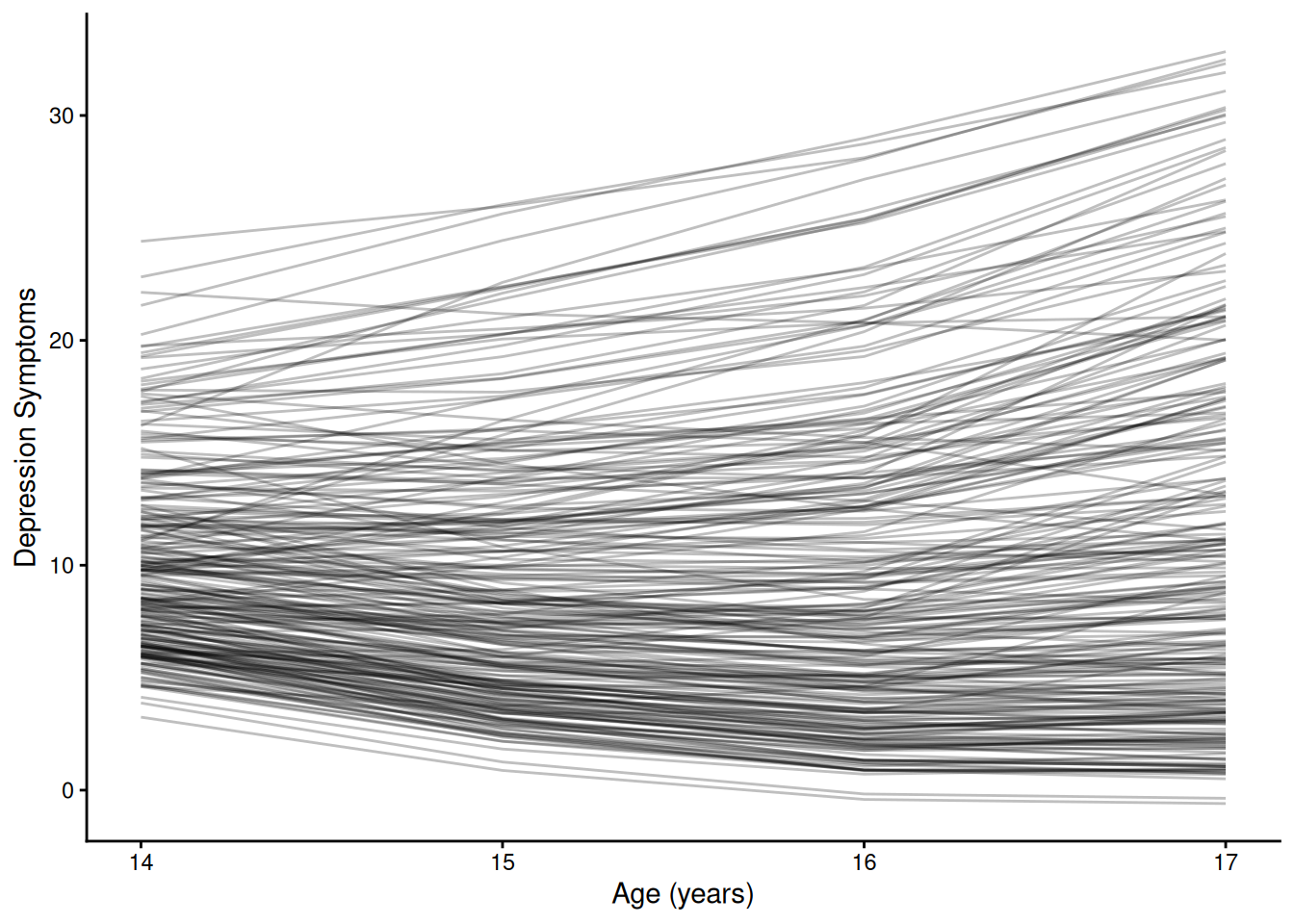
Code
ggplot(
  data = modelPredictedValues_long,
  mapping = aes(
    x = time,
    y = anxiety,
    group = ID)) +
  geom_line(
    alpha = 0.25
  ) +
  labs(
    x = "Age (years)",
    y = "Anxiety Symptoms"
  ) +
  theme_classic()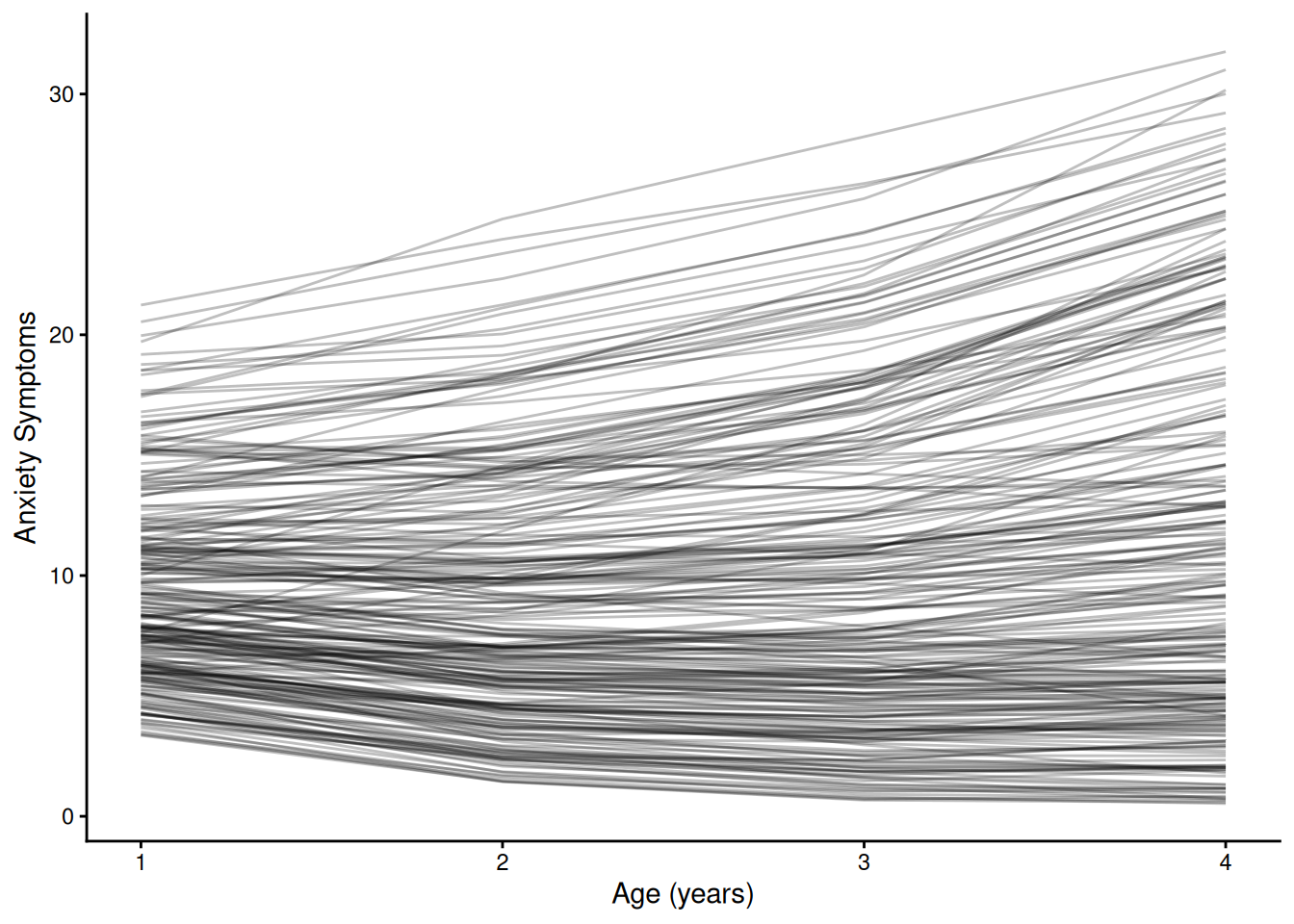
7 Cross-Lagged Panel Model
7.1 Model Syntax
This cross-lagged panel model examines whether anxiety predicts later depression (i.e., cross-lagged paths), controlling for prior levels of depression (i.e., autoregressive effects), and simultaneously examines the reverse association (i.e., depression predicting later anxiety, controlling for prior levels of anxiety). Concurrent covariances between depression and anxiety at each timepoint account for shared variance at the same occasion.
Code
clpm_syntax <- '
  # Autoregressive Paths
  depression_4 ~ depression_3
  depression_3 ~ depression_2
  depression_2 ~ depression_1

  anxiety_4 ~ anxiety_3
  anxiety_3 ~ anxiety_2
  anxiety_2 ~ anxiety_1

  # Concurrent Covariances
  depression_1 ~~ anxiety_1
  depression_2 ~~ anxiety_2
  depression_3 ~~ anxiety_3
  depression_4 ~~ anxiety_4

  # Cross-Lagged Paths
  depression_4 ~ anxiety_3
  depression_3 ~ anxiety_2
  depression_2 ~ anxiety_1

  anxiety_4 ~ depression_3
  anxiety_3 ~ depression_2
  anxiety_2 ~ depression_1
'
7.2 Fit Model
Code
clpm_fit <- lavaan::sem(
  clpm_syntax,
  data = mydata_wide,
  missing = "ML", # FIML
  estimator = "MLR", # Huber-White robust standard errors (for heteroscedasticity and nonnormally distributed residuals)
  meanstructure = TRUE, # estimate means/intercepts
  fixed.x = FALSE) # estimate means, variances, and covariances of the observed variables (to include predictors as part of FIML)
7.3 Model Summary
Code
summary(
  clpm_fit,
  fit.measures = TRUE,
  standardized = TRUE,
  rsquare = TRUE)
lavaan 0.6-21 ended normally after 90 iterations
Estimator ML
Optimization method NLMINB
Number of model parameters 32
Number of observations 250
Number of missing patterns 6
Model Test User Model:
Standard Scaled
Test Statistic 50.696 36.849
Degrees of freedom 12 12
P-value (Chi-square) 0.000 0.000
Scaling correction factor 1.376
Yuan-Bentler correction (Mplus variant)
Model Test Baseline Model:
Test statistic 2762.171 1772.854
Degrees of freedom 28 28
P-value 0.000 0.000
Scaling correction factor 1.558
User Model versus Baseline Model:
Comparative Fit Index (CFI) 0.986 0.986
Tucker-Lewis Index (TLI) 0.967 0.967
Robust Comparative Fit Index (CFI) 0.986
Robust Tucker-Lewis Index (TLI) 0.968
Loglikelihood and Information Criteria:
Loglikelihood user model (H0) -4668.395 -4668.395
Scaling correction factor 1.353
for the MLR correction
Loglikelihood unrestricted model (H1) -4643.048 -4643.048
Scaling correction factor 1.359
for the MLR correction
Akaike (AIC) 9400.791 9400.791
Bayesian (BIC) 9513.478 9513.478
Sample-size adjusted Bayesian (SABIC) 9412.035 9412.035
Root Mean Square Error of Approximation:
RMSEA 0.114 0.091
90 Percent confidence interval - lower 0.082 0.063
90 Percent confidence interval - upper 0.147 0.120
P-value H_0: RMSEA <= 0.050 0.001 0.010
P-value H_0: RMSEA >= 0.080 0.961 0.759
Robust RMSEA 0.118
90 Percent confidence interval - lower 0.077
90 Percent confidence interval - upper 0.162
P-value H_0: Robust RMSEA <= 0.050 0.005
P-value H_0: Robust RMSEA >= 0.080 0.936
Standardized Root Mean Square Residual:
SRMR 0.013 0.013
Parameter Estimates:
Standard errors Sandwich
Information bread Observed
Observed information based on Hessian
Regressions:
Estimate Std.Err z-value P(>|z|) Std.lv Std.all
depression_4 ~
depression_3 1.039 0.048 21.564 0.000 1.039 0.836
depression_3 ~
depression_2 1.030 0.040 25.534 0.000 1.030 0.852
depression_2 ~
depression_1 1.042 0.052 20.215 0.000 1.042 0.793
anxiety_4 ~
anxiety_3 1.051 0.054 19.485 0.000 1.051 0.833
anxiety_3 ~
anxiety_2 1.043 0.056 18.591 0.000 1.043 0.862
anxiety_2 ~
anxiety_1 1.066 0.062 17.237 0.000 1.066 0.824
depression_4 ~
anxiety_3 0.187 0.047 3.939 0.000 0.187 0.148
depression_3 ~
anxiety_2 0.167 0.036 4.661 0.000 0.167 0.136
depression_2 ~
anxiety_1 0.226 0.052 4.315 0.000 0.226 0.172
anxiety_4 ~
depression_3 0.142 0.053 2.660 0.008 0.142 0.114
anxiety_3 ~
depression_2 0.092 0.060 1.530 0.126 0.092 0.077
anxiety_2 ~
depression_1 0.024 0.056 0.428 0.669 0.024 0.019
Covariances:
Estimate Std.Err z-value P(>|z|) Std.lv Std.all
depression_1 ~~
anxiety_1 10.388 1.396 7.442 0.000 10.388 0.535
.depression_2 ~~
.anxiety_2 4.463 0.655 6.819 0.000 4.463 0.553
.depression_3 ~~
.anxiety_3 2.849 0.546 5.216 0.000 2.849 0.448
.depression_4 ~~
.anxiety_4 4.293 0.877 4.895 0.000 4.293 0.455
Intercepts:
Estimate Std.Err z-value P(>|z|) Std.lv Std.all
.depression_4 -0.511 0.261 -1.956 0.050 -0.511 -0.059
.depression_3 -1.600 0.268 -5.974 0.000 -1.600 -0.229
.depression_2 -3.594 0.419 -8.587 0.000 -3.594 -0.621
.anxiety_4 -0.079 0.296 -0.268 0.789 -0.079 -0.009
.anxiety_3 -0.701 0.344 -2.036 0.042 -0.701 -0.101
.anxiety_2 -1.355 0.519 -2.609 0.009 -1.355 -0.237
depression_1 10.152 0.278 36.458 0.000 10.152 2.306
anxiety_1 9.576 0.279 34.323 0.000 9.576 2.171
Variances:
Estimate Std.Err z-value P(>|z|) Std.lv Std.all
.depression_4 7.477 1.010 7.403 0.000 7.477 0.099
.depression_3 5.142 0.752 6.842 0.000 5.142 0.105
.depression_2 6.560 0.716 9.164 0.000 6.560 0.196
.anxiety_4 11.922 1.717 6.942 0.000 11.922 0.157
.anxiety_3 7.854 0.994 7.901 0.000 7.854 0.165
.anxiety_2 9.931 1.187 8.367 0.000 9.931 0.305
depression_1 19.385 1.878 10.322 0.000 19.385 1.000
anxiety_1 19.460 1.607 12.109 0.000 19.460 1.000
R-Square:
Estimate
depression_4 0.901
depression_3 0.895
depression_2 0.804
anxiety_4 0.843
anxiety_3 0.835
anxiety_2 0.6957.4 Modification Indices
Code
modificationindices(
  clpm_fit,
  sort. = TRUE)
7.5 Plots
7.5.1 Path Diagram
Code
lavaanPlot::lavaanPlot(
  clpm_fit,
  coefs = TRUE,
  #covs = TRUE,
  stand = TRUE)
Path Diagram
To create an interactive path diagram, you can use the following syntax:
Code
lavaangui::plot_lavaan(clpm_fit)8 Random-Intercepts Cross-Lagged Panel Model
Adapted from:
- Mulder & Hamaker (2021): https://doi.org/10.1080/10705511.2020.1784738
- Mund & Nestler (2017): https://osf.io/a4dhk
8.1 Model Syntax
This random-intercepts cross-lagged panel model examines whether anxiety predicts later depression (i.e., cross-lagged paths), controlling for prior levels of depression (i.e., autoregressive effects) and controlling for a person’s general latent level of depression, and simultaneously and simultaneously examines the reverse association (i.e., depression predicting later anxiety, controlling for prior levels of anxiety and general latent levels of anxiety). Concurrent covariances between depression and anxiety at each timepoint account for shared variance at the same occasion.
Code
riclpm_syntax <- '
  # Random Intercepts
  depression =~ 1*depression_1 + 1*depression_2 + 1*depression_3 + 1*depression_4
  anxiety =~ 1*anxiety_1 + 1*anxiety_2 + 1*anxiety_3 + 1*anxiety_4

  # Create Within-Person Centered Variables
  wdep1 =~ 1*depression_1
  wdep2 =~ 1*depression_2
  wdep3 =~ 1*depression_3
  wdep4 =~ 1*depression_4

  wanx1 =~ 1*anxiety_1
  wanx2 =~ 1*anxiety_2
  wanx3 =~ 1*anxiety_3
  wanx4 =~ 1*anxiety_4

  # Autoregressive Paths
  wdep4 ~ wdep3
  wdep3 ~ wdep2
  wdep2 ~ wdep1

  wanx4 ~ wanx3
  wanx3 ~ wanx2
  wanx2 ~ wanx1

  # Concurrent Covariances
  wdep1 ~~ wanx1
  wdep2 ~~ wanx2
  wdep3 ~~ wanx3
  wdep4 ~~ wanx4

  # Cross-Lagged Paths
  wdep4 ~ wanx3
  wdep3 ~ wanx2
  wdep2 ~ wanx1

  wanx4 ~ wdep3
  wanx3 ~ wdep2
  wanx2 ~ wdep1

  # Variance and Covariance of Random Intercepts
  depression ~~ depression
  anxiety ~~ anxiety
  depression ~~ anxiety

  # Variances of Within-Person Centered Variables
  wdep1 ~~ wdep1
  wdep2 ~~ wdep2
  wdep3 ~~ wdep3
  wdep4 ~~ wdep4

  wanx1 ~~ wanx1
  wanx2 ~~ wanx2
  wanx3 ~~ wanx3
  wanx4 ~~ wanx4

  # Fix Error Variances of Observed Variables to Zero
  depression_1 ~~ 0*depression_1
  depression_2 ~~ 0*depression_2
  depression_3 ~~ 0*depression_3
  depression_4 ~~ 0*depression_4

  anxiety_1 ~~ 0*anxiety_1
  anxiety_2 ~~ 0*anxiety_2
  anxiety_3 ~~ 0*anxiety_3
  anxiety_4 ~~ 0*anxiety_4

  # Fix the Covariances Between the Random Intercepts and the Latents at T1 to Zero
  wdep1 ~~ 0*depression
  wdep1 ~~ 0*anxiety

  wanx1 ~~ 0*depression
  wanx1 ~~ 0*anxiety

  # Estimate Observed Intercepts
  depression_1 ~ 1
  depression_2 ~ 1
  depression_3 ~ 1
  depression_4 ~ 1

  anxiety_1 ~ 1
  anxiety_2 ~ 1
  anxiety_3 ~ 1
  anxiety_4 ~ 1

  # Fix the Means of the Latents to Zero
  wdep1 ~ 0*1
  wdep2 ~ 0*1
  wdep3 ~ 0*1
  wdep4 ~ 0*1

  wanx1 ~ 0*1
  wanx2 ~ 0*1
  wanx3 ~ 0*1
  wanx4 ~ 0*1

  depression ~ 0*1
  anxiety ~ 0*1
'
8.2 Fit Model
Code
riclpm_fit <- lavaan::sem(
  riclpm_syntax,
  data = mydata_wide,
  missing = "ML", # FIML
  estimator = "MLR", # Huber-White robust standard errors (for heteroscedasticity and nonnormally distributed residuals)
  fixed.x = FALSE, # estimate means, variances, and covariances of the observed variables (to include predictors as part of FIML)
  bounds = "standard" # constrains observed variances, latent variances, and factor loadings to be within computed lower and upper bounds
)
Warning: lavaan->lav_object_post_check():
covariance matrix of latent variables is not positive definite ; use
lavInspect(fit, "cov.lv") to investigate.Modify the syntax to address the model fit errors (don’t estimate concurrent covariances):
Code
riclpm2_syntax <- '
  # Random Intercepts
  depression =~ 1*depression_1 + 1*depression_2 + 1*depression_3 + 1*depression_4
  anxiety =~ 1*anxiety_1 + 1*anxiety_2 + 1*anxiety_3 + 1*anxiety_4

  # Create Within-Person Centered Variables
  wdep1 =~ 1*depression_1
  wdep2 =~ 1*depression_2
  wdep3 =~ 1*depression_3
  wdep4 =~ 1*depression_4

  wanx1 =~ 1*anxiety_1
  wanx2 =~ 1*anxiety_2
  wanx3 =~ 1*anxiety_3
  wanx4 =~ 1*anxiety_4

  # Autoregressive Paths
  wdep4 ~ wdep3
  wdep3 ~ wdep2
  wdep2 ~ wdep1

  wanx4 ~ wanx3
  wanx3 ~ wanx2
  wanx2 ~ wanx1

  # Concurrent Covariances
  #wdep1 ~~ wanx1
  #wdep2 ~~ wanx2
  #wdep3 ~~ wanx3
  #wdep4 ~~ wanx4

  # Cross-Lagged Paths
  wdep4 ~ wanx3
  wdep3 ~ wanx2
  wdep2 ~ wanx1

  wanx4 ~ wdep3
  wanx3 ~ wdep2
  wanx2 ~ wdep1

  # Variance and Covariance of Random Intercepts
  depression ~~ depression
  anxiety ~~ anxiety
  depression ~~ anxiety

  # Variances of Within-Person Centered Variables
  wdep1 ~~ wdep1
  wdep2 ~~ wdep2
  wdep3 ~~ wdep3
  wdep4 ~~ wdep4

  wanx1 ~~ wanx1
  wanx2 ~~ wanx2
  wanx3 ~~ wanx3
  wanx4 ~~ wanx4

  # Fix Error Variances of Observed Variables to Zero
  depression_1 ~~ 0*depression_1
  depression_2 ~~ 0*depression_2
  depression_3 ~~ 0*depression_3
  depression_4 ~~ 0*depression_4

  anxiety_1 ~~ 0*anxiety_1
  anxiety_2 ~~ 0*anxiety_2
  anxiety_3 ~~ 0*anxiety_3
  anxiety_4 ~~ 0*anxiety_4

  # Fix the Covariances Between the Random Intercepts and the Latents at T1 to Zero
  wdep1 ~~ 0*depression
  wdep1 ~~ 0*anxiety

  wanx1 ~~ 0*depression
  wanx1 ~~ 0*anxiety

  # Estimate Observed Intercepts
  depression_1 ~ 1
  depression_2 ~ 1
  depression_3 ~ 1
  depression_4 ~ 1

  anxiety_1 ~ 1
  anxiety_2 ~ 1
  anxiety_3 ~ 1
  anxiety_4 ~ 1

  # Fix the Means of the Latents to Zero
  wdep1 ~ 0*1
  wdep2 ~ 0*1
  wdep3 ~ 0*1
  wdep4 ~ 0*1

  wanx1 ~ 0*1
  wanx2 ~ 0*1
  wanx3 ~ 0*1
  wanx4 ~ 0*1

  depression ~ 0*1
  anxiety ~ 0*1
'

riclpm2_fit <- lavaan::sem(
  riclpm2_syntax,
  data = mydata_wide,
  missing = "ML", # FIML
  estimator = "MLR", # Huber-White robust standard errors (for heteroscedasticity and nonnormally distributed residuals)
  fixed.x = FALSE, # estimate means, variances, and covariances of the observed variables (to include predictors as part of FIML)
  bounds = "standard" # constrains observed variances, latent variances, and factor loadings to be within computed lower and upper bounds
)
8.3 Model Summary
Code
summary(
  riclpm2_fit,
  fit.measures = TRUE,
  standardized = TRUE,
  rsquare = TRUE)
lavaan 0.6-21 ended normally after 245 iterations
Estimator ML
Optimization method NLMINB
Number of model parameters 33
Row rank of the constraints matrix 13
Number of observations 250
Number of missing patterns 6
Model Test User Model:
Standard Scaled
Test Statistic 221.074 146.651
Degrees of freedom 11 11
P-value (Chi-square) 0.000 0.000
Scaling correction factor 1.507
Yuan-Bentler correction (Mplus variant)
Model Test Baseline Model:
Test statistic 2762.171 1772.854
Degrees of freedom 28 28
P-value 0.000 0.000
Scaling correction factor 1.558
User Model versus Baseline Model:
Comparative Fit Index (CFI) 0.923 0.922
Tucker-Lewis Index (TLI) 0.804 0.802
Robust Comparative Fit Index (CFI) 0.929
Robust Tucker-Lewis Index (TLI) 0.820
Loglikelihood and Information Criteria:
Loglikelihood user model (H0) -4753.585 -4753.585
Scaling correction factor 1.310
for the MLR correction
Loglikelihood unrestricted model (H1) -4643.048 -4643.048
Scaling correction factor 1.359
for the MLR correction
Akaike (AIC) 9573.170 9573.170
Bayesian (BIC) 9689.378 9689.378
Sample-size adjusted Bayesian (SABIC) 9584.765 9584.765
Root Mean Square Error of Approximation:
RMSEA 0.276 0.222
90 Percent confidence interval - lower 0.245 0.197
90 Percent confidence interval - upper 0.309 0.249
P-value H_0: RMSEA <= 0.050 0.000 0.000
P-value H_0: RMSEA >= 0.080 1.000 1.000
Robust RMSEA 0.280
90 Percent confidence interval - lower 0.240
90 Percent confidence interval - upper 0.322
P-value H_0: Robust RMSEA <= 0.050 0.000
P-value H_0: Robust RMSEA >= 0.080 1.000
Standardized Root Mean Square Residual:
SRMR 0.275 0.275
Parameter Estimates:
Standard errors Sandwich
Information bread Observed
Observed information based on Hessian
Latent Variables:
Estimate Std.Err z-value P(>|z|) Std.lv Std.all
depression =~
depression_1 1.000 5.802 0.900
depression_2 1.000 5.802 1.000
depression_3 1.000 5.802 0.920
depression_4 1.000 5.802 0.799
anxiety =~
anxiety_1 1.000 3.359 0.799
anxiety_2 1.000 3.359 0.658
anxiety_3 1.000 3.359 0.546
anxiety_4 1.000 3.359 0.434
wdep1 =~
depression_1 1.000 2.805 0.435
wdep2 =~
depression_2 1.000 0.078 0.013
wdep3 =~
depression_3 1.000 2.476 0.393
wdep4 =~
depression_4 1.000 4.372 0.602
wanx1 =~
anxiety_1 1.000 2.528 0.601
wanx2 =~
anxiety_2 1.000 3.850 0.753
wanx3 =~
anxiety_3 1.000 5.157 0.838
wanx4 =~
anxiety_4 1.000 6.974 0.901
Regressions:
Estimate Std.Err z-value P(>|z|) Std.lv Std.all
wdep4 ~
wdep3 0.842 0.129 6.509 0.000 0.477 0.477
wdep3 ~
wdep2 -13.387 6.703 -1.997 0.046 -0.421 -0.421
wdep2 ~
wdep1 0.007 0.006 1.174 0.240 0.242 0.242
wanx4 ~
wanx3 1.150 0.084 13.640 0.000 0.850 0.850
wanx3 ~
wanx2 0.874 0.105 8.301 0.000 0.652 0.652
wanx2 ~
wanx1 0.812 0.129 6.304 0.000 0.533 0.533
wdep4 ~
wanx3 0.327 0.069 4.759 0.000 0.385 0.385
wdep3 ~
wanx2 0.216 0.087 2.483 0.013 0.336 0.336
wdep2 ~
wanx1 -0.010 0.006 -1.741 0.082 -0.319 -0.319
wanx4 ~
wdep3 0.032 0.183 0.176 0.861 0.011 0.011
wanx3 ~
wdep2 -38.764 16.158 -2.399 0.016 -0.585 -0.585
wanx2 ~
wdep1 -0.632 0.064 -9.841 0.000 -0.460 -0.460
Covariances:
Estimate Std.Err z-value P(>|z|) Std.lv Std.all
depression ~~
anxiety 13.022 2.536 5.135 0.000 0.668 0.668
wdep1 0.000 0.000 0.000
anxiety ~~
wdep1 0.000 0.000 0.000
depression ~~
wanx1 0.000 0.000 0.000
anxiety ~~
wanx1 0.000 0.000 0.000
wdep1 ~~
wanx1 -0.599 0.982 -0.610 0.542 -0.085 -0.085
.wdep4 ~~
.wanx4 4.883 0.969 5.039 0.000 0.492 0.492
Intercepts:
Estimate Std.Err z-value P(>|z|) Std.lv Std.all
.depression_1 10.152 0.278 36.458 0.000 10.152 1.575
.depression_2 9.151 0.367 24.938 0.000 9.151 1.577
.depression_3 9.335 0.443 21.065 0.000 9.335 1.480
.depression_4 11.007 0.554 19.864 0.000 11.007 1.515
.anxiety_1 9.576 0.279 34.323 0.000 9.576 2.278
.anxiety_2 9.100 0.362 25.166 0.000 9.100 1.781
.anxiety_3 9.618 0.437 21.993 0.000 9.618 1.563
.anxiety_4 11.395 0.561 20.308 0.000 11.395 1.472
wdep1 0.000 0.000 0.000
.wdep2 0.000 0.000 0.000
.wdep3 0.000 0.000 0.000
.wdep4 0.000 0.000 0.000
wanx1 0.000 0.000 0.000
.wanx2 0.000 0.000 0.000
.wanx3 0.000 0.000 0.000
.wanx4 0.000 0.000 0.000
depression 0.000 0.000 0.000
anxiety 0.000 0.000 0.000
Variances:
Estimate Std.Err z-value P(>|z|) Std.lv Std.all
depressin 33.661 3.615 9.311 0.000 1.000 1.000
anxiety 11.285 3.536 3.192 0.001 1.000 1.000
wdep1 7.865 0.909 8.651 0.000 1.000 1.000
.wdep2 (lb) 0.005 0.004 1.256 0.827 0.827
.wdep3 3.824 0.671 5.701 0.000 0.624 0.624
.wdep4 7.652 0.982 7.795 0.000 0.400 0.400
wanx1 6.389 2.812 2.272 0.023 1.000 1.000
.wanx2 6.850 0.929 7.373 0.000 0.462 0.462
.wanx3 (lb) 0.005 2.457 0.002 0.000 0.000
.wanx4 12.882 1.855 6.943 0.000 0.265 0.265
.deprssn_1 0.000 0.000 0.000
.deprssn_2 0.000 0.000 0.000
.deprssn_3 0.000 0.000 0.000
.deprssn_4 0.000 0.000 0.000
.anxiety_1 0.000 0.000 0.000
.anxiety_2 0.000 0.000 0.000
.anxiety_3 0.000 0.000 0.000
.anxiety_4 0.000 0.000 0.000
R-Square:
Estimate
wdep2 0.173
wdep3 0.376
wdep4 0.600
wanx2 0.538
wanx3 1.000
wanx4 0.735
depression_1 1.000
depression_2 1.000
depression_3 1.000
depression_4 1.000
anxiety_1 1.000
anxiety_2 1.000
anxiety_3 1.000
anxiety_4 1.0008.4 Modification Indices
Code
modificationindices(
  riclpm2_fit,
  sort. = TRUE)
8.5 Path Diagram
Code
lavaanPlot::lavaanPlot(
  riclpm2_fit,
  coefs = TRUE,
  #covs = TRUE,
  stand = TRUE)
To create an interactive path diagram, you can use the following syntax:
Code
lavaangui::plot_lavaan(riclpm2_fit)9 Multilevel SEM
9.1 Model Syntax
This multilevel structural equation model disaggregates within- and between-person effects to examine associations with depression. At the within-person level, we examine deviations in sleep, anxiety, and SES from a person’s usual (average) levels in predicting concurrent deviations in depression, allowing the within-person association between sleep and depression to differ between boys and girls. At the between-person level, we examine person-level averages across time of sleep, anxiety, and SES, along with sex, in predicting overall differences in depression across individuals, allowing the between-person association between sleep and depression to differ between boys and girls.
Code
multilevelSEM_syntax <- '
    level: 1
        depression ~ sleep_personMeanCentered + anxiety_personMeanCentered + ses_personMeanCentered + sexEffectCodeXsleep_personMeanCentered
    level: 2
        depression ~ sleep_personMean + anxiety_personMean + ses_personMean + sexEffectCode + sexEffectCodeXsleep_personMean
'
9.2 Fit Model
Code
multilevelSEM_fit <- lavaan::sem(
  multilevelSEM_syntax,
  data = mydata_long,
  cluster = "ID",
  missing = "ML", # FIML
  estimator = "MLR")
9.3 Model Summary
Code
summary(
  multilevelSEM_fit,
  fit.measures = TRUE,
  standardized = TRUE,
  rsquare = TRUE)
lavaan 0.6-21 ended normally after 59 iterations
Estimator ML
Optimization method NLMINB
Number of model parameters 12
Used Total
Number of observations 931 1000
Number of clusters [ID] 250
Number of missing patterns -- level 1 1
Number of missing patterns -- level 2 1
Model Test User Model:
Standard Scaled
Test Statistic 0.000 0.000
Degrees of freedom 0 0
Model Test Baseline Model:
Test statistic 900.477 725.220
Degrees of freedom 9 9
P-value 0.000 0.000
Scaling correction factor 1.242
User Model versus Baseline Model:
Comparative Fit Index (CFI) 1.000 1.000
Tucker-Lewis Index (TLI) 1.000 1.000
Robust Comparative Fit Index (CFI) NA
Robust Tucker-Lewis Index (TLI) NA
Loglikelihood and Information Criteria:
Loglikelihood user model (H0) -2349.089 -2349.089
Loglikelihood unrestricted model (H1) -2349.090 -2349.090
Akaike (AIC) 4722.178 4722.178
Bayesian (BIC) 4780.213 4780.213
Sample-size adjusted Bayesian (SABIC) 4742.102 4742.102
Root Mean Square Error of Approximation:
RMSEA 0.000 NA
90 Percent confidence interval - lower 0.000 NA
90 Percent confidence interval - upper 0.000 NA
P-value H_0: RMSEA <= 0.050 NA NA
P-value H_0: RMSEA >= 0.080 NA NA
Robust RMSEA NA
90 Percent confidence interval - lower NA
90 Percent confidence interval - upper NA
P-value H_0: Robust RMSEA <= 0.050 NA
P-value H_0: Robust RMSEA >= 0.080 NA
Standardized Root Mean Square Residual (corr metric):
SRMR (within covariance matrix) 0.000 0.000
SRMR (between covariance matrix) 0.001 0.001
Parameter Estimates:
Standard errors Sandwich
Information bread Observed
Observed information based on Hessian
Level 1 [within]:
Regressions:
Estimate Std.Err z-value P(>|z|) Std.lv Std.all
depression ~
slp_prsnMnCntr -0.498 0.154 -3.239 0.001 -0.498 -0.107
anxty_prsnMnCn 0.632 0.038 16.645 0.000 0.632 0.615
ss_prsnMnCntrd 0.338 0.177 1.909 0.056 0.338 0.059
sxEffctCdXs_MC 0.020 0.126 0.155 0.876 0.020 0.004
Variances:
Estimate Std.Err z-value P(>|z|) Std.lv Std.all
.depression 4.555 0.365 12.463 0.000 4.555 0.602
R-Square:
Estimate
depression 0.398
Level 2 [ID]:
Regressions:
Estimate Std.Err z-value P(>|z|) Std.lv Std.all
depression ~
sleep_personMn -0.500 0.393 -1.274 0.203 -0.500 -0.081
anxiety_prsnMn 0.631 0.055 11.556 0.000 0.631 0.627
ses_personMean -0.857 0.419 -2.042 0.041 -0.857 -0.125
sexEffectCode -3.338 2.516 -1.327 0.185 -3.338 -0.552
sxEffctCdXsl_M 0.304 0.311 0.979 0.328 0.304 0.407
Intercepts:
Estimate Std.Err z-value P(>|z|) Std.lv Std.all
.depression 7.582 3.200 2.370 0.018 7.582 1.264
Variances:
Estimate Std.Err z-value P(>|z|) Std.lv Std.all
.depression 15.028 1.806 8.319 0.000 15.028 0.418
R-Square:
Estimate
depression 0.5829.4 Modification Indices
Code
modificationindices(
  multilevelSEM_fit,
  sort. = TRUE)
9.5 Path Diagram
Code
lavaanPlot::lavaanPlot(
  multilevelSEM_fit,
  coefs = TRUE,
  #covs = TRUE,
  stand = TRUE)
To create an interactive path diagram, you can use the following syntax:
Code
lavaangui::plot_lavaan(multilevelSEM_fit)10 Longitudinal Measurement Invariance
We will follow the approach suggested by Widaman et al. (2010).
Widaman, K. F., Ferrer, E., & Conger, R. D. (2010). Factorial invariance within longitudinal structural equation models: Measuring the same construct across time. Child Development Perspectives, 4(1), 10–18. https://doi.org/10.1111/j.1750-8606.2009.00110.x
For the longitudinal measurement invariance models, we will use simulated data from https://mycourses.aalto.fi/mod/assign/view.php?id=1203047 (archived at https://perma.cc/QTL2-ZHX2). These data were simulated and adapted from data from Bliese and Ployhart (2002):
Bliese, P. D., & Ployhart, R. E. (2002). Growth modeling using random coefficient models: Model building, testing, and illustrations. Organizational Research Methods, 5(4), 362–387. https://doi.org/10.1177/109442802237116
As noted here (archived at https://perma.cc/QTL2-ZHX2), “The data are in wide format where the variables are coded as [VARIABLE NAME][time index][indicator index].” The data include three indicators for each of three constructs: 1) job satisfaction (JOBSAT), 2) organizational commitment (COMMIT), and 3) readiness to perform (READY).
Questions:
- Which level of longitudinal measurement invariance holds for the
Bliese-Ployhart-2002-indicators-1.csvdataset (saved in objectlongitudinalMI1)? - Repeat the tests of longitudinal measurement invariance for the remaining datasets:
Bliese-Ployhart-2000-indicators-2.csv,Bliese-Ployhart-2000-indicators-3.csv, andBliese-Ployhart-2000-indicators-4.csv. Which level of longitudinal measurement invariance holds for each dataset?
The answers to these questions are here.
10.1 Configural Invariance
A configural invariance model has the same number of latent factors across time, with the indicators loading onto the same latent factor(s) across time. Model fit indices can then be examined to evaluate how tenable it is that (a) there are the same number of latent factors across time and that (b) the indicators load onto the same latent factor(s) across time.
- Standardize the latent factor(s) at T1 (i.e., fix the mean to zero and the variance to one)
- For each latent construct, constrain the first indicator’s factor loading to be the same across time
- For each latent construct, constrain the first indicator’s intercept to be the same across time
10.1.1 Model Syntax
Code
configuralInvariance_syntax <- '
  # Factor Loadings
  jobsat_1 =~ NA*loadj1*JOBSAT11 + JOBSAT12 + JOBSAT13
  jobsat_2 =~ NA*loadj1*JOBSAT21 + JOBSAT22 + JOBSAT23
  jobsat_3 =~ NA*loadj1*JOBSAT31 + JOBSAT32 + JOBSAT33

  ready_1 =~ NA*loadr1*READY11 + READY12 + READY13
  ready_2 =~ NA*loadr1*READY21 + READY22 + READY23
  ready_3 =~ NA*loadr1*READY31 + READY32 + READY33

  commit_1 =~ NA*loadc1*COMMIT11 + COMMIT12 + COMMIT13
  commit_2 =~ NA*loadc1*COMMIT21 + COMMIT22 + COMMIT23
  commit_3 =~ NA*loadc1*COMMIT31 + COMMIT32 + COMMIT33

  # Factor Identification: Standardize Factors at T1

  ## Fix Factor Means at T1 to Zero
  jobsat_1 ~ 0*1
  ready_1 ~ 0*1
  commit_1 ~ 0*1

  ## Fix Factor Variances at T1 to One
  jobsat_1 ~~ 1*jobsat_1
  ready_1 ~~ 1*ready_1
  commit_1 ~~ 1*commit_1

  # Freely Estimate Factor Means at T2 and T3 (relative to T1)
  jobsat_2 ~ 1
  jobsat_3 ~ 1

  ready_2 ~ 1
  ready_3 ~ 1

  commit_2 ~ 1
  commit_3 ~ 1

  # Freely Estimate Factor Variances at T2 and T3 (relative to T1)
  jobsat_2 ~~ jobsat_2
  jobsat_3 ~~ jobsat_3

  ready_2 ~~ ready_2
  ready_3 ~~ ready_3

  commit_2 ~~ commit_2
  commit_3 ~~ commit_3

  # Fix Intercepts of Indicator 1 Across Time
  JOBSAT11 ~ intj1*1
  JOBSAT21 ~ intj1*1
  JOBSAT31 ~ intj1*1

  READY11 ~ intr1*1
  READY21 ~ intr1*1
  READY31 ~ intr1*1

  COMMIT11 ~ intc1*1
  COMMIT21 ~ intc1*1
  COMMIT31 ~ intc1*1

  # Free Intercepts of Remaining Manifest Variables
  JOBSAT12 ~ 1
  JOBSAT13 ~ 1
  JOBSAT22 ~ 1
  JOBSAT23 ~ 1
  JOBSAT32 ~ 1
  JOBSAT33 ~ 1

  READY12 ~ 1
  READY13 ~ 1
  READY22 ~ 1
  READY23 ~ 1
  READY32 ~ 1
  READY33 ~ 1

  COMMIT12 ~ 1
  COMMIT13 ~ 1
  COMMIT22 ~ 1
  COMMIT23 ~ 1
  COMMIT32 ~ 1
  COMMIT33 ~ 1

  # Estimate Residual Variances of Manifest Variables
  JOBSAT11 ~~ JOBSAT11
  JOBSAT12 ~~ JOBSAT12
  JOBSAT13 ~~ JOBSAT13
  JOBSAT21 ~~ JOBSAT21
  JOBSAT22 ~~ JOBSAT22
  JOBSAT23 ~~ JOBSAT23
  JOBSAT31 ~~ JOBSAT31
  JOBSAT32 ~~ JOBSAT32
  JOBSAT33 ~~ JOBSAT33

  READY11 ~~ READY11
  READY12 ~~ READY12
  READY13 ~~ READY13
  READY21 ~~ READY21
  READY22 ~~ READY22
  READY23 ~~ READY23
  READY31 ~~ READY31
  READY32 ~~ READY32
  READY33 ~~ READY33

  COMMIT11 ~~ COMMIT11
  COMMIT12 ~~ COMMIT12
  COMMIT13 ~~ COMMIT13
  COMMIT21 ~~ COMMIT21
  COMMIT22 ~~ COMMIT22
  COMMIT23 ~~ COMMIT23
  COMMIT31 ~~ COMMIT31
  COMMIT32 ~~ COMMIT32
  COMMIT33 ~~ COMMIT33
'
10.1.2 Fit Model
Code
configuralInvariance_fit <- cfa(
  configuralInvariance_syntax,
  data = longitudinalMI1,
  missing = "ML", # FIML
  estimator = "MLR", # Huber-White robust standard errors (for heteroscedasticity and nonnormally distributed residuals)
  meanstructure = TRUE, # estimate means/intercepts
  fixed.x = FALSE) # estimate means, variances, and covariances of the observed variables (to include predictors as part of FIML)
10.1.3 Model Summary
Code
summary(
  configuralInvariance_fit,
  fit.measures = TRUE,
  standardized = TRUE,
  rsquare = TRUE)
lavaan 0.6-21 ended normally after 101 iterations
Estimator ML
Optimization method NLMINB
Number of model parameters 129
Number of equality constraints 12
Number of observations 495
Number of missing patterns 1
Model Test User Model:
Standard Scaled
Test Statistic 770.816 783.291
Degrees of freedom 288 288
P-value (Chi-square) 0.000 0.000
Scaling correction factor 0.984
Yuan-Bentler correction (Mplus variant)
Model Test Baseline Model:
Test statistic 6697.063 6541.933
Degrees of freedom 351 351
P-value 0.000 0.000
Scaling correction factor 1.024
User Model versus Baseline Model:
Comparative Fit Index (CFI) 0.924 0.920
Tucker-Lewis Index (TLI) 0.907 0.902
Robust Comparative Fit Index (CFI) 0.923
Robust Tucker-Lewis Index (TLI) 0.906
Loglikelihood and Information Criteria:
Loglikelihood user model (H0) -17716.771 -17716.771
Scaling correction factor 0.935
for the MLR correction
Loglikelihood unrestricted model (H1) -17331.363 -17331.363
Scaling correction factor 0.998
for the MLR correction
Akaike (AIC) 35667.543 35667.543
Bayesian (BIC) 36159.476 36159.476
Sample-size adjusted Bayesian (SABIC) 35788.115 35788.115
Root Mean Square Error of Approximation:
RMSEA 0.058 0.059
90 Percent confidence interval - lower 0.053 0.054
90 Percent confidence interval - upper 0.063 0.064
P-value H_0: RMSEA <= 0.050 0.003 0.002
P-value H_0: RMSEA >= 0.080 0.000 0.000
Robust RMSEA 0.058
90 Percent confidence interval - lower 0.054
90 Percent confidence interval - upper 0.063
P-value H_0: Robust RMSEA <= 0.050 0.002
P-value H_0: Robust RMSEA >= 0.080 0.000
Standardized Root Mean Square Residual:
SRMR 0.032 0.032
Parameter Estimates:
Standard errors Sandwich
Information bread Observed
Observed information based on Hessian
Latent Variables:
Estimate Std.Err z-value P(>|z|) Std.lv Std.all
jobsat_1 =~
JOBSAT1 (ldj1) 0.996 0.041 24.099 0.000 0.996 0.818
JOBSAT1 1.019 0.042 24.487 0.000 1.019 0.814
JOBSAT1 0.956 0.040 23.787 0.000 0.956 0.798
jobsat_2 =~
JOBSAT2 (ldj1) 0.996 0.041 24.099 0.000 0.961 0.796
JOBSAT2 1.001 0.058 17.194 0.000 0.967 0.805
JOBSAT2 0.964 0.064 15.021 0.000 0.931 0.785
jobsat_3 =~
JOBSAT3 (ldj1) 0.996 0.041 24.099 0.000 0.861 0.776
JOBSAT3 0.980 0.066 14.839 0.000 0.848 0.773
JOBSAT3 1.070 0.071 15.159 0.000 0.926 0.806
ready_1 =~
READY11 (ldr1) 0.900 0.042 21.255 0.000 0.900 0.781
READY12 0.882 0.043 20.311 0.000 0.882 0.766
READY13 0.905 0.041 21.860 0.000 0.905 0.789
ready_2 =~
READY21 (ldr1) 0.900 0.042 21.255 0.000 0.947 0.795
READY22 0.785 0.053 14.924 0.000 0.826 0.731
READY23 0.821 0.056 14.581 0.000 0.864 0.750
ready_3 =~
READY31 (ldr1) 0.900 0.042 21.255 0.000 0.878 0.764
READY32 0.847 0.062 13.766 0.000 0.827 0.750
READY33 0.888 0.070 12.759 0.000 0.867 0.757
commit_1 =~
COMMIT1 (ldc1) 0.809 0.044 18.389 0.000 0.809 0.748
COMMIT1 0.825 0.041 19.985 0.000 0.825 0.755
COMMIT1 0.815 0.042 19.477 0.000 0.815 0.753
commit_2 =~
COMMIT2 (ldc1) 0.809 0.044 18.389 0.000 0.854 0.768
COMMIT2 0.818 0.058 14.105 0.000 0.863 0.768
COMMIT2 0.866 0.062 13.866 0.000 0.914 0.787
commit_3 =~
COMMIT3 (ldc1) 0.809 0.044 18.389 0.000 0.774 0.752
COMMIT3 0.771 0.059 13.123 0.000 0.738 0.706
COMMIT3 0.812 0.066 12.398 0.000 0.777 0.728
Covariances:
Estimate Std.Err z-value P(>|z|) Std.lv Std.all
jobsat_1 ~~
jobsat_2 0.436 0.058 7.532 0.000 0.451 0.451
jobsat_3 0.325 0.052 6.288 0.000 0.375 0.375
ready_1 0.542 0.050 10.840 0.000 0.542 0.542
ready_2 0.286 0.062 4.611 0.000 0.271 0.271
ready_3 0.176 0.057 3.105 0.002 0.181 0.181
commit_1 0.581 0.046 12.496 0.000 0.581 0.581
commit_2 0.380 0.063 6.086 0.000 0.360 0.360
commit_3 0.237 0.056 4.211 0.000 0.248 0.248
jobsat_2 ~~
jobsat_3 0.381 0.057 6.665 0.000 0.456 0.456
ready_1 0.198 0.057 3.494 0.000 0.205 0.205
ready_2 0.508 0.067 7.574 0.000 0.500 0.500
ready_3 0.193 0.057 3.405 0.001 0.205 0.205
commit_1 0.278 0.055 5.049 0.000 0.288 0.288
commit_2 0.584 0.070 8.297 0.000 0.573 0.573
commit_3 0.260 0.059 4.431 0.000 0.281 0.281
jobsat_3 ~~
ready_1 0.201 0.048 4.224 0.000 0.232 0.232
ready_2 0.272 0.054 5.051 0.000 0.298 0.298
ready_3 0.451 0.063 7.182 0.000 0.534 0.534
commit_1 0.182 0.052 3.489 0.000 0.210 0.210
commit_2 0.265 0.059 4.503 0.000 0.290 0.290
commit_3 0.480 0.061 7.885 0.000 0.580 0.580
ready_1 ~~
ready_2 0.404 0.066 6.073 0.000 0.383 0.383
ready_3 0.323 0.059 5.445 0.000 0.331 0.331
commit_1 0.452 0.050 9.057 0.000 0.452 0.452
commit_2 0.282 0.065 4.332 0.000 0.267 0.267
commit_3 0.230 0.058 3.990 0.000 0.240 0.240
ready_2 ~~
ready_3 0.515 0.077 6.723 0.000 0.501 0.501
commit_1 0.270 0.062 4.373 0.000 0.256 0.256
commit_2 0.694 0.086 8.052 0.000 0.625 0.625
commit_3 0.309 0.066 4.709 0.000 0.307 0.307
ready_3 ~~
commit_1 0.175 0.059 2.981 0.003 0.180 0.180
commit_2 0.298 0.067 4.478 0.000 0.289 0.289
commit_3 0.452 0.070 6.414 0.000 0.484 0.484
commit_1 ~~
commit_2 0.632 0.065 9.669 0.000 0.598 0.598
commit_3 0.427 0.059 7.214 0.000 0.447 0.447
commit_2 ~~
commit_3 0.583 0.090 6.510 0.000 0.577 0.577
Intercepts:
Estimate Std.Err z-value P(>|z|) Std.lv Std.all
jbst_1 0.000 0.000 0.000
redy_1 0.000 0.000 0.000
cmmt_1 0.000 0.000 0.000
jbst_2 -0.000 0.062 -0.000 1.000 -0.000 -0.000
jbst_3 0.126 0.060 2.099 0.036 0.145 0.145
redy_2 0.056 0.070 0.802 0.422 0.053 0.053
redy_3 0.204 0.073 2.818 0.005 0.209 0.209
cmmt_2 -0.200 0.069 -2.885 0.004 -0.189 -0.189
cmmt_3 -0.172 0.071 -2.442 0.015 -0.180 -0.180
.JOBSAT (intj1) 3.319 0.055 60.662 0.000 3.319 2.727
.JOBSAT (intj1) 3.319 0.055 60.662 0.000 3.319 2.749
.JOBSAT (intj1) 3.319 0.055 60.662 0.000 3.319 2.989
.READY1 (intr1) 3.176 0.052 61.297 0.000 3.176 2.755
.READY2 (intr1) 3.176 0.052 61.297 0.000 3.176 2.665
.READY3 (intr1) 3.176 0.052 61.297 0.000 3.176 2.763
.COMMIT (intc1) 3.719 0.049 76.578 0.000 3.719 3.442
.COMMIT (intc1) 3.719 0.049 76.578 0.000 3.719 3.345
.COMMIT (intc1) 3.719 0.049 76.578 0.000 3.719 3.613
.JOBSAT 3.311 0.056 58.833 0.000 3.311 2.644
.JOBSAT 3.321 0.054 61.701 0.000 3.321 2.773
.JOBSAT 3.331 0.067 49.733 0.000 3.331 2.774
.JOBSAT 3.329 0.067 49.620 0.000 3.329 2.805
.JOBSAT 3.281 0.065 50.616 0.000 3.281 2.992
.JOBSAT 3.251 0.070 46.441 0.000 3.251 2.830
.READY1 3.198 0.052 61.778 0.000 3.198 2.777
.READY1 3.156 0.052 61.219 0.000 3.156 2.752
.READY2 3.170 0.061 51.554 0.000 3.170 2.807
.READY2 3.211 0.062 51.499 0.000 3.211 2.788
.READY3 3.156 0.066 47.871 0.000 3.156 2.864
.READY3 3.146 0.070 44.635 0.000 3.146 2.747
.COMMIT 3.653 0.049 74.420 0.000 3.653 3.345
.COMMIT 3.596 0.049 73.962 0.000 3.596 3.324
.COMMIT 3.689 0.064 57.387 0.000 3.689 3.282
.COMMIT 3.662 0.066 55.846 0.000 3.662 3.153
.COMMIT 3.749 0.061 61.081 0.000 3.749 3.586
.COMMIT 3.692 0.064 57.657 0.000 3.692 3.457
Variances:
Estimate Std.Err z-value P(>|z|) Std.lv Std.all
jobsat_1 1.000 1.000 1.000
ready_1 1.000 1.000 1.000
commit_1 1.000 1.000 1.000
jobsat_2 0.933 0.098 9.534 0.000 1.000 1.000
jobsat_3 0.748 0.087 8.650 0.000 1.000 1.000
ready_2 1.108 0.122 9.097 0.000 1.000 1.000
ready_3 0.952 0.122 7.786 0.000 1.000 1.000
commit_2 1.114 0.146 7.615 0.000 1.000 1.000
commit_3 0.916 0.127 7.204 0.000 1.000 1.000
.JOBSAT11 0.491 0.051 9.630 0.000 0.491 0.331
.JOBSAT12 0.529 0.049 10.895 0.000 0.529 0.337
.JOBSAT13 0.521 0.046 11.315 0.000 0.521 0.363
.JOBSAT21 0.533 0.052 10.209 0.000 0.533 0.366
.JOBSAT22 0.506 0.047 10.685 0.000 0.506 0.351
.JOBSAT23 0.542 0.052 10.394 0.000 0.542 0.384
.JOBSAT31 0.491 0.042 11.704 0.000 0.491 0.398
.JOBSAT32 0.484 0.043 11.164 0.000 0.484 0.403
.JOBSAT33 0.463 0.046 10.128 0.000 0.463 0.350
.READY11 0.519 0.051 10.112 0.000 0.519 0.391
.READY12 0.548 0.048 11.392 0.000 0.548 0.413
.READY13 0.496 0.048 10.318 0.000 0.496 0.377
.READY21 0.522 0.054 9.742 0.000 0.522 0.368
.READY22 0.593 0.049 12.067 0.000 0.593 0.465
.READY23 0.580 0.055 10.611 0.000 0.580 0.437
.READY31 0.550 0.054 10.190 0.000 0.550 0.417
.READY32 0.531 0.048 11.179 0.000 0.531 0.437
.READY33 0.560 0.048 11.585 0.000 0.560 0.427
.COMMIT11 0.514 0.050 10.191 0.000 0.514 0.440
.COMMIT12 0.512 0.045 11.266 0.000 0.512 0.429
.COMMIT13 0.506 0.047 10.756 0.000 0.506 0.432
.COMMIT21 0.508 0.046 10.932 0.000 0.508 0.411
.COMMIT22 0.518 0.047 11.112 0.000 0.518 0.410
.COMMIT23 0.513 0.051 10.121 0.000 0.513 0.380
.COMMIT31 0.461 0.043 10.761 0.000 0.461 0.435
.COMMIT32 0.548 0.054 10.095 0.000 0.548 0.501
.COMMIT33 0.536 0.048 11.080 0.000 0.536 0.470
R-Square:
Estimate
JOBSAT11 0.669
JOBSAT12 0.663
JOBSAT13 0.637
JOBSAT21 0.634
JOBSAT22 0.649
JOBSAT23 0.616
JOBSAT31 0.602
JOBSAT32 0.597
JOBSAT33 0.650
READY11 0.609
READY12 0.587
READY13 0.623
READY21 0.632
READY22 0.535
READY23 0.563
READY31 0.583
READY32 0.563
READY33 0.573
COMMIT11 0.560
COMMIT12 0.571
COMMIT13 0.568
COMMIT21 0.589
COMMIT22 0.590
COMMIT23 0.620
COMMIT31 0.565
COMMIT32 0.499
COMMIT33 0.53010.1.4 Modification Indices
Code
modificationindices(
  configuralInvariance_fit,
  sort. = TRUE)
10.1.5 Path Diagram
Code
lavaanPlot::lavaanPlot2(
  configuralInvariance_fit,
  stand = TRUE,
  coef_labels = TRUE)
Path Diagram
To create an interactive path diagram, you can use the following syntax:
Code
lavaangui::plot_lavaan(configuralInvariance_fit)10.3 Metric (“Weak Factorial”) Invariance
A metric invariance model evaluates whether the items’ factor loadings are the same across time.
- Standardize the latent factor(s) at T1 (i.e., fix the mean to zero and the variance to one)
- For each latent construct, constrain the first indicator’s intercept to be the same across time
- Allow within-indicator residuals to covary across time
- For each indicator, constrain its factor loading to be the same across time
10.3.1 Model Syntax
Code
metricInvariance_syntax <- '
  # Factor Loadings
  jobsat_1 =~ NA*loadj1*JOBSAT11 + loadj2*JOBSAT12 + loadj3*JOBSAT13
  jobsat_2 =~ NA*loadj1*JOBSAT21 + loadj2*JOBSAT22 + loadj3*JOBSAT23
  jobsat_3 =~ NA*loadj1*JOBSAT31 + loadj2*JOBSAT32 + loadj3*JOBSAT33

  ready_1 =~ NA*loadr1*READY11 + loadr2*READY12 + loadr3*READY13
  ready_2 =~ NA*loadr1*READY21 + loadr2*READY22 + loadr3*READY23
  ready_3 =~ NA*loadr1*READY31 + loadr2*READY32 + loadr3*READY33

  commit_1 =~ NA*loadc1*COMMIT11 + loadc2*COMMIT12 + loadc3*COMMIT13
  commit_2 =~ NA*loadc1*COMMIT21 + loadc2*COMMIT22 + loadc3*COMMIT23
  commit_3 =~ NA*loadc1*COMMIT31 + loadc2*COMMIT32 + loadc3*COMMIT33

  # Factor Identification: Standardize Factors at T1

  ## Fix Factor Means at T1 to Zero
  jobsat_1 ~ 0*1
  ready_1 ~ 0*1
  commit_1 ~ 0*1

  ## Fix Factor Variances at T1 to One
  jobsat_1 ~~ 1*jobsat_1
  ready_1 ~~ 1*ready_1
  commit_1 ~~ 1*commit_1

  # Freely Estimate Factor Means at T2 and T3 (relative to T1)
  jobsat_2 ~ 1
  jobsat_3 ~ 1

  ready_2 ~ 1
  ready_3 ~ 1

  commit_2 ~ 1
  commit_3 ~ 1

  # Freely Estimate Factor Variances at T2 and T3 (relative to T1)
  jobsat_2 ~~ jobsat_2
  jobsat_3 ~~ jobsat_3

  ready_2 ~~ ready_2
  ready_3 ~~ ready_3

  commit_2 ~~ commit_2
  commit_3 ~~ commit_3

  # Fix Intercepts of Indicator 1 Across Time
  JOBSAT11 ~ intj1*1
  JOBSAT21 ~ intj1*1
  JOBSAT31 ~ intj1*1

  READY11 ~ intr1*1
  READY21 ~ intr1*1
  READY31 ~ intr1*1

  COMMIT11 ~ intc1*1
  COMMIT21 ~ intc1*1
  COMMIT31 ~ intc1*1

  # Free Intercepts of Remaining Manifest Variables
  JOBSAT12 ~ 1
  JOBSAT13 ~ 1
  JOBSAT22 ~ 1
  JOBSAT23 ~ 1
  JOBSAT32 ~ 1
  JOBSAT33 ~ 1

  READY12 ~ 1
  READY13 ~ 1
  READY22 ~ 1
  READY23 ~ 1
  READY32 ~ 1
  READY33 ~ 1

  COMMIT12 ~ 1
  COMMIT13 ~ 1
  COMMIT22 ~ 1
  COMMIT23 ~ 1
  COMMIT32 ~ 1
  COMMIT33 ~ 1

  # Estimate Residual Variances of Manifest Variables
  JOBSAT11 ~~ JOBSAT11
  JOBSAT12 ~~ JOBSAT12
  JOBSAT13 ~~ JOBSAT13
  JOBSAT21 ~~ JOBSAT21
  JOBSAT22 ~~ JOBSAT22
  JOBSAT23 ~~ JOBSAT23
  JOBSAT31 ~~ JOBSAT31
  JOBSAT32 ~~ JOBSAT32
  JOBSAT33 ~~ JOBSAT33

  READY11 ~~ READY11
  READY12 ~~ READY12
  READY13 ~~ READY13
  READY21 ~~ READY21
  READY22 ~~ READY22
  READY23 ~~ READY23
  READY31 ~~ READY31
  READY32 ~~ READY32
  READY33 ~~ READY33

  COMMIT11 ~~ COMMIT11
  COMMIT12 ~~ COMMIT12
  COMMIT13 ~~ COMMIT13
  COMMIT21 ~~ COMMIT21
  COMMIT22 ~~ COMMIT22
  COMMIT23 ~~ COMMIT23
  COMMIT31 ~~ COMMIT31
  COMMIT32 ~~ COMMIT32
  COMMIT33 ~~ COMMIT33

  # Residual Covariances Within Indicator Across Time
  JOBSAT11 ~~ JOBSAT21
  JOBSAT21 ~~ JOBSAT31
  JOBSAT11 ~~ JOBSAT31

  JOBSAT12 ~~ JOBSAT22
  JOBSAT22 ~~ JOBSAT32
  JOBSAT12 ~~ JOBSAT32

  JOBSAT13 ~~ JOBSAT23
  JOBSAT23 ~~ JOBSAT33
  JOBSAT13 ~~ JOBSAT33

  READY11 ~~ READY21
  READY21 ~~ READY31
  READY11 ~~ READY31

  READY12 ~~ READY22
  READY22 ~~ READY32
  READY12 ~~ READY32

  READY13 ~~ READY23
  READY23 ~~ READY33
  READY13 ~~ READY33

  COMMIT11 ~~ COMMIT21
  COMMIT21 ~~ COMMIT31
  COMMIT11 ~~ COMMIT31

  COMMIT12 ~~ COMMIT22
  COMMIT22 ~~ COMMIT32
  COMMIT12 ~~ COMMIT32

  COMMIT13 ~~ COMMIT23
  COMMIT23 ~~ COMMIT33
  COMMIT13 ~~ COMMIT33
'
10.3.2 Fit Model
Code
metricInvariance_fit <- cfa(
  metricInvariance_syntax,
  data = longitudinalMI1,
  missing = "ML", # FIML
  estimator = "MLR", # Huber-White robust standard errors (for heteroscedasticity and nonnormally distributed residuals)
  meanstructure = TRUE, # estimate means/intercepts
  fixed.x = FALSE) # estimate means, variances, and covariances of the observed variables (to include predictors as part of FIML)
10.3.3 Model Summary
Code
summary(
  metricInvariance_fit,
  fit.measures = TRUE,
  standardized = TRUE,
  rsquare = TRUE)
lavaan 0.6-21 ended normally after 91 iterations
Estimator ML
Optimization method NLMINB
Number of model parameters 156
Number of equality constraints 24
Number of observations 495
Number of missing patterns 1
Model Test User Model:
Standard Scaled
Test Statistic 286.159 292.814
Degrees of freedom 273 273
P-value (Chi-square) 0.280 0.196
Scaling correction factor 0.977
Yuan-Bentler correction (Mplus variant)
Model Test Baseline Model:
Test statistic 6697.063 6541.933
Degrees of freedom 351 351
P-value 0.000 0.000
Scaling correction factor 1.024
User Model versus Baseline Model:
Comparative Fit Index (CFI) 0.998 0.997
Tucker-Lewis Index (TLI) 0.997 0.996
Robust Comparative Fit Index (CFI) 0.997
Robust Tucker-Lewis Index (TLI) 0.996
Loglikelihood and Information Criteria:
Loglikelihood user model (H0) -17474.443 -17474.443
Scaling correction factor 0.880
for the MLR correction
Loglikelihood unrestricted model (H1) -17331.363 -17331.363
Scaling correction factor 0.998
for the MLR correction
Akaike (AIC) 35212.885 35212.885
Bayesian (BIC) 35767.887 35767.887
Sample-size adjusted Bayesian (SABIC) 35348.916 35348.916
Root Mean Square Error of Approximation:
RMSEA 0.010 0.012
90 Percent confidence interval - lower 0.000 0.000
90 Percent confidence interval - upper 0.021 0.022
P-value H_0: RMSEA <= 0.050 1.000 1.000
P-value H_0: RMSEA >= 0.080 0.000 0.000
Robust RMSEA 0.012
90 Percent confidence interval - lower 0.000
90 Percent confidence interval - upper 0.022
P-value H_0: Robust RMSEA <= 0.050 1.000
P-value H_0: Robust RMSEA >= 0.080 0.000
Standardized Root Mean Square Residual:
SRMR 0.024 0.024
Parameter Estimates:
Standard errors Sandwich
Information bread Observed
Observed information based on Hessian
Latent Variables:
Estimate Std.Err z-value P(>|z|) Std.lv Std.all
jobsat_1 =~
JOBSAT1 (ldj1) 0.974 0.036 26.751 0.000 0.974 0.807
JOBSAT1 (ldj2) 0.995 0.035 28.661 0.000 0.995 0.801
JOBSAT1 (ldj3) 0.995 0.036 27.941 0.000 0.995 0.819
jobsat_2 =~
JOBSAT2 (ldj1) 0.974 0.036 26.751 0.000 0.937 0.781
JOBSAT2 (ldj2) 0.995 0.035 28.661 0.000 0.957 0.803
JOBSAT2 (ldj3) 0.995 0.036 27.941 0.000 0.957 0.797
jobsat_3 =~
JOBSAT3 (ldj1) 0.974 0.036 26.751 0.000 0.866 0.778
JOBSAT3 (ldj2) 0.995 0.035 28.661 0.000 0.884 0.793
JOBSAT3 (ldj3) 0.995 0.036 27.941 0.000 0.884 0.783
ready_1 =~
READY11 (ldr1) 0.930 0.036 25.486 0.000 0.930 0.797
READY12 (ldr2) 0.850 0.036 23.877 0.000 0.850 0.748
READY13 (ldr3) 0.899 0.036 24.965 0.000 0.899 0.785
ready_2 =~
READY21 (ldr1) 0.930 0.036 25.486 0.000 0.916 0.779
READY22 (ldr2) 0.850 0.036 23.877 0.000 0.837 0.737
READY23 (ldr3) 0.899 0.036 24.965 0.000 0.886 0.763
ready_3 =~
READY31 (ldr1) 0.930 0.036 25.486 0.000 0.893 0.773
READY32 (ldr2) 0.850 0.036 23.877 0.000 0.816 0.743
READY33 (ldr3) 0.899 0.036 24.965 0.000 0.864 0.756
commit_1 =~
COMMIT1 (ldc1) 0.807 0.036 22.195 0.000 0.807 0.749
COMMIT1 (ldc2) 0.807 0.036 22.194 0.000 0.807 0.744
COMMIT1 (ldc3) 0.826 0.036 22.787 0.000 0.826 0.759
commit_2 =~
COMMIT2 (ldc1) 0.807 0.036 22.195 0.000 0.870 0.778
COMMIT2 (ldc2) 0.807 0.036 22.194 0.000 0.870 0.773
COMMIT2 (ldc3) 0.826 0.036 22.787 0.000 0.891 0.773
commit_3 =~
COMMIT3 (ldc1) 0.807 0.036 22.195 0.000 0.758 0.741
COMMIT3 (ldc2) 0.807 0.036 22.194 0.000 0.758 0.720
COMMIT3 (ldc3) 0.826 0.036 22.787 0.000 0.776 0.727
Covariances:
Estimate Std.Err z-value P(>|z|) Std.lv Std.all
.JOBSAT11 ~~
.JOBSAT21 0.118 0.032 3.655 0.000 0.118 0.222
.JOBSAT21 ~~
.JOBSAT31 0.123 0.032 3.905 0.000 0.123 0.235
.JOBSAT11 ~~
.JOBSAT31 0.151 0.029 5.126 0.000 0.151 0.303
.JOBSAT12 ~~
.JOBSAT22 0.155 0.034 4.560 0.000 0.155 0.293
.JOBSAT22 ~~
.JOBSAT32 0.095 0.030 3.160 0.002 0.095 0.196
.JOBSAT12 ~~
.JOBSAT32 0.075 0.032 2.345 0.019 0.075 0.148
.JOBSAT13 ~~
.JOBSAT23 0.090 0.033 2.714 0.007 0.090 0.179
.JOBSAT23 ~~
.JOBSAT33 0.147 0.033 4.402 0.000 0.147 0.290
.JOBSAT13 ~~
.JOBSAT33 0.114 0.031 3.647 0.000 0.114 0.233
.READY11 ~~
.READY21 0.136 0.033 4.094 0.000 0.136 0.262
.READY21 ~~
.READY31 0.107 0.032 3.357 0.001 0.107 0.198
.READY11 ~~
.READY31 0.099 0.033 2.987 0.003 0.099 0.191
.READY12 ~~
.READY22 0.181 0.033 5.396 0.000 0.181 0.312
.READY22 ~~
.READY32 0.173 0.037 4.647 0.000 0.173 0.306
.READY12 ~~
.READY32 0.120 0.034 3.548 0.000 0.120 0.217
.READY13 ~~
.READY23 0.133 0.033 4.032 0.000 0.133 0.251
.READY23 ~~
.READY33 0.168 0.035 4.860 0.000 0.168 0.300
.READY13 ~~
.READY33 0.117 0.033 3.586 0.000 0.117 0.220
.COMMIT11 ~~
.COMMIT21 0.122 0.032 3.872 0.000 0.122 0.244
.COMMIT21 ~~
.COMMIT31 0.142 0.031 4.587 0.000 0.142 0.294
.COMMIT11 ~~
.COMMIT31 0.110 0.029 3.732 0.000 0.110 0.225
.COMMIT12 ~~
.COMMIT22 0.101 0.032 3.144 0.002 0.101 0.194
.COMMIT22 ~~
.COMMIT32 0.119 0.033 3.576 0.000 0.119 0.228
.COMMIT12 ~~
.COMMIT32 0.084 0.031 2.743 0.006 0.084 0.159
.COMMIT13 ~~
.COMMIT23 0.171 0.034 5.073 0.000 0.171 0.329
.COMMIT23 ~~
.COMMIT33 0.150 0.031 4.856 0.000 0.150 0.279
.COMMIT13 ~~
.COMMIT33 0.111 0.033 3.399 0.001 0.111 0.213
jobsat_1 ~~
jobsat_2 0.388 0.054 7.125 0.000 0.403 0.403
jobsat_3 0.292 0.050 5.802 0.000 0.328 0.328
ready_1 0.541 0.050 10.817 0.000 0.541 0.541
ready_2 0.272 0.057 4.748 0.000 0.276 0.276
ready_3 0.175 0.055 3.167 0.002 0.182 0.182
commit_1 0.580 0.047 12.416 0.000 0.580 0.580
commit_2 0.388 0.061 6.394 0.000 0.360 0.360
commit_3 0.230 0.054 4.230 0.000 0.245 0.245
jobsat_2 ~~
jobsat_3 0.348 0.052 6.634 0.000 0.407 0.407
ready_1 0.200 0.056 3.585 0.000 0.208 0.208
ready_2 0.480 0.060 8.037 0.000 0.507 0.507
ready_3 0.191 0.054 3.512 0.000 0.206 0.206
commit_1 0.278 0.055 5.091 0.000 0.289 0.289
commit_2 0.595 0.068 8.732 0.000 0.574 0.574
commit_3 0.254 0.057 4.415 0.000 0.281 0.281
jobsat_3 ~~
ready_1 0.206 0.047 4.372 0.000 0.232 0.232
ready_2 0.264 0.051 5.190 0.000 0.302 0.302
ready_3 0.454 0.056 8.182 0.000 0.532 0.532
commit_1 0.192 0.052 3.674 0.000 0.216 0.216
commit_2 0.283 0.058 4.889 0.000 0.295 0.295
commit_3 0.486 0.056 8.666 0.000 0.582 0.582
ready_1 ~~
ready_2 0.316 0.061 5.203 0.000 0.320 0.320
ready_3 0.270 0.056 4.797 0.000 0.281 0.281
commit_1 0.455 0.050 9.178 0.000 0.455 0.455
commit_2 0.289 0.064 4.502 0.000 0.268 0.268
commit_3 0.223 0.056 3.994 0.000 0.237 0.237
ready_2 ~~
ready_3 0.413 0.061 6.751 0.000 0.437 0.437
commit_1 0.255 0.057 4.444 0.000 0.259 0.259
commit_2 0.660 0.071 9.283 0.000 0.622 0.622
commit_3 0.282 0.058 4.863 0.000 0.305 0.305
ready_3 ~~
commit_1 0.175 0.058 3.031 0.002 0.182 0.182
commit_2 0.303 0.063 4.776 0.000 0.293 0.293
commit_3 0.435 0.060 7.264 0.000 0.482 0.482
commit_1 ~~
commit_2 0.579 0.059 9.790 0.000 0.537 0.537
commit_3 0.369 0.056 6.590 0.000 0.393 0.393
commit_2 ~~
commit_3 0.518 0.075 6.929 0.000 0.511 0.511
Intercepts:
Estimate Std.Err z-value P(>|z|) Std.lv Std.all
jbst_1 0.000 0.000 0.000
redy_1 0.000 0.000 0.000
cmmt_1 0.000 0.000 0.000
jbst_2 0.000 0.063 0.000 1.000 0.000 0.000
jbst_3 0.129 0.061 2.103 0.035 0.145 0.145
redy_2 0.054 0.068 0.801 0.423 0.055 0.055
redy_3 0.198 0.070 2.818 0.005 0.206 0.206
cmmt_2 -0.200 0.068 -2.937 0.003 -0.186 -0.186
cmmt_3 -0.173 0.070 -2.473 0.013 -0.184 -0.184
.JOBSAT (intj1) 3.319 0.055 60.662 0.000 3.319 2.751
.JOBSAT (intj1) 3.319 0.055 60.662 0.000 3.319 2.767
.JOBSAT (intj1) 3.319 0.055 60.662 0.000 3.319 2.984
.READY1 (intr1) 3.176 0.052 61.296 0.000 3.176 2.722
.READY2 (intr1) 3.176 0.052 61.296 0.000 3.176 2.701
.READY3 (intr1) 3.176 0.052 61.296 0.000 3.176 2.747
.COMMIT (intc1) 3.719 0.049 76.578 0.000 3.719 3.454
.COMMIT (intc1) 3.719 0.049 76.578 0.000 3.719 3.326
.COMMIT (intc1) 3.719 0.049 76.578 0.000 3.719 3.639
.JOBSAT 3.311 0.056 58.833 0.000 3.311 2.668
.JOBSAT 3.321 0.054 61.701 0.000 3.321 2.734
.JOBSAT 3.331 0.068 49.283 0.000 3.331 2.796
.JOBSAT 3.329 0.069 48.075 0.000 3.329 2.775
.JOBSAT 3.276 0.065 50.125 0.000 3.276 2.939
.JOBSAT 3.258 0.067 48.848 0.000 3.258 2.885
.READY1 3.198 0.052 61.778 0.000 3.198 2.816
.READY1 3.156 0.052 61.219 0.000 3.156 2.755
.READY2 3.168 0.063 50.350 0.000 3.168 2.787
.READY2 3.208 0.064 49.907 0.000 3.208 2.765
.READY3 3.161 0.064 49.723 0.000 3.161 2.877
.READY3 3.150 0.067 46.681 0.000 3.150 2.756
.COMMIT 3.653 0.049 74.419 0.000 3.653 3.368
.COMMIT 3.596 0.049 73.962 0.000 3.596 3.302
.COMMIT 3.687 0.063 58.086 0.000 3.687 3.273
.COMMIT 3.654 0.065 56.470 0.000 3.654 3.171
.COMMIT 3.756 0.063 59.858 0.000 3.756 3.565
.COMMIT 3.694 0.065 57.102 0.000 3.694 3.458
Variances:
Estimate Std.Err z-value P(>|z|) Std.lv Std.all
jobsat_1 1.000 1.000 1.000
ready_1 1.000 1.000 1.000
commit_1 1.000 1.000 1.000
jobsat_2 0.925 0.070 13.235 0.000 1.000 1.000
jobsat_3 0.789 0.068 11.639 0.000 1.000 1.000
ready_2 0.971 0.083 11.740 0.000 1.000 1.000
ready_3 0.922 0.082 11.302 0.000 1.000 1.000
commit_2 1.163 0.113 10.320 0.000 1.000 1.000
commit_3 0.882 0.092 9.612 0.000 1.000 1.000
.JOBSAT11 0.507 0.048 10.579 0.000 0.507 0.348
.JOBSAT12 0.551 0.046 11.972 0.000 0.551 0.358
.JOBSAT13 0.486 0.044 10.964 0.000 0.486 0.329
.JOBSAT21 0.561 0.049 11.404 0.000 0.561 0.390
.JOBSAT22 0.505 0.047 10.776 0.000 0.505 0.355
.JOBSAT23 0.524 0.050 10.578 0.000 0.524 0.364
.JOBSAT31 0.488 0.040 12.241 0.000 0.488 0.394
.JOBSAT32 0.462 0.040 11.493 0.000 0.462 0.371
.JOBSAT33 0.494 0.044 11.169 0.000 0.494 0.387
.READY11 0.496 0.049 10.188 0.000 0.496 0.364
.READY12 0.567 0.045 12.740 0.000 0.567 0.440
.READY13 0.504 0.045 11.200 0.000 0.504 0.384
.READY21 0.543 0.050 10.947 0.000 0.543 0.393
.READY22 0.591 0.049 12.168 0.000 0.591 0.457
.READY23 0.561 0.051 10.951 0.000 0.561 0.417
.READY31 0.539 0.050 10.779 0.000 0.539 0.403
.READY32 0.540 0.046 11.793 0.000 0.540 0.448
.READY33 0.560 0.044 12.583 0.000 0.560 0.429
.COMMIT11 0.509 0.048 10.659 0.000 0.509 0.439
.COMMIT12 0.525 0.044 11.823 0.000 0.525 0.446
.COMMIT13 0.503 0.046 10.913 0.000 0.503 0.424
.COMMIT21 0.494 0.045 10.965 0.000 0.494 0.395
.COMMIT22 0.512 0.047 10.936 0.000 0.512 0.403
.COMMIT23 0.535 0.049 10.865 0.000 0.535 0.402
.COMMIT31 0.470 0.041 11.504 0.000 0.470 0.450
.COMMIT32 0.535 0.052 10.214 0.000 0.535 0.482
.COMMIT33 0.539 0.046 11.644 0.000 0.539 0.472
R-Square:
Estimate
JOBSAT11 0.652
JOBSAT12 0.642
JOBSAT13 0.671
JOBSAT21 0.610
JOBSAT22 0.645
JOBSAT23 0.636
JOBSAT31 0.606
JOBSAT32 0.629
JOBSAT33 0.613
READY11 0.636
READY12 0.560
READY13 0.616
READY21 0.607
READY22 0.543
READY23 0.583
READY31 0.597
READY32 0.552
READY33 0.571
COMMIT11 0.561
COMMIT12 0.554
COMMIT13 0.576
COMMIT21 0.605
COMMIT22 0.597
COMMIT23 0.598
COMMIT31 0.550
COMMIT32 0.518
COMMIT33 0.52810.3.4 Modification Indices
Code
modificationindices(
  metricInvariance_fit,
  sort. = TRUE)
10.3.5 Path Diagram
Code
lavaanPlot::lavaanPlot2(
  metricInvariance_fit,
  stand = TRUE,
  coef_labels = TRUE)
Path Diagram
To create an interactive path diagram, you can use the following syntax:
Code
lavaangui::plot_lavaan(metricInvariance_fit)10.3.6 Compare Models
Code
anova(
  configuralInvarianceCorrelatedResiduals_fit,
  metricInvariance_fit
)
10.4 Scalar (“Strong Factorial”) Invariance
A scalar invariance model evaluates whether the items’ intercepts are the same across time.
- Standardize the latent factor(s) at T1 (i.e., fix the mean to zero and the variance to one)
- Allow within-indicator residuals to covary across time
- For each indicator, constrain its factor loading to be the same across time
- For each indicator, constrain its intercept to be the same across time
10.4.1 Model Syntax
Code
scalarInvariance_syntax <- '
  # Factor Loadings
  jobsat_1 =~ NA*loadj1*JOBSAT11 + loadj2*JOBSAT12 + loadj3*JOBSAT13
  jobsat_2 =~ NA*loadj1*JOBSAT21 + loadj2*JOBSAT22 + loadj3*JOBSAT23
  jobsat_3 =~ NA*loadj1*JOBSAT31 + loadj2*JOBSAT32 + loadj3*JOBSAT33

  ready_1 =~ NA*loadr1*READY11 + loadr2*READY12 + loadr3*READY13
  ready_2 =~ NA*loadr1*READY21 + loadr2*READY22 + loadr3*READY23
  ready_3 =~ NA*loadr1*READY31 + loadr2*READY32 + loadr3*READY33

  commit_1 =~ NA*loadc1*COMMIT11 + loadc2*COMMIT12 + loadc3*COMMIT13
  commit_2 =~ NA*loadc1*COMMIT21 + loadc2*COMMIT22 + loadc3*COMMIT23
  commit_3 =~ NA*loadc1*COMMIT31 + loadc2*COMMIT32 + loadc3*COMMIT33

  # Factor Identification: Standardize Factors at T1

  ## Fix Factor Means at T1 to Zero
  jobsat_1 ~ 0*1
  ready_1 ~ 0*1
  commit_1 ~ 0*1

  ## Fix Factor Variances at T1 to One
  jobsat_1 ~~ 1*jobsat_1
  ready_1 ~~ 1*ready_1
  commit_1 ~~ 1*commit_1

  # Freely Estimate Factor Means at T2 and T3 (relative to T1)
  jobsat_2 ~ 1
  jobsat_3 ~ 1

  ready_2 ~ 1
  ready_3 ~ 1

  commit_2 ~ 1
  commit_3 ~ 1

  # Freely Estimate Factor Variances at T2 and T3 (relative to T1)
  jobsat_2 ~~ jobsat_2
  jobsat_3 ~~ jobsat_3

  ready_2 ~~ ready_2
  ready_3 ~~ ready_3

  commit_2 ~~ commit_2
  commit_3 ~~ commit_3

  # Fix Intercepts of Indicators Across Time
  JOBSAT11 ~ intj1*1
  JOBSAT21 ~ intj1*1
  JOBSAT31 ~ intj1*1
  JOBSAT12 ~ intj2*1
  JOBSAT22 ~ intj2*1
  JOBSAT32 ~ intj2*1
  JOBSAT13 ~ intj3*1
  JOBSAT23 ~ intj3*1
  JOBSAT33 ~ intj3*1

  READY11 ~ intr1*1
  READY21 ~ intr1*1
  READY31 ~ intr1*1
  READY12 ~ intr2*1
  READY22 ~ intr2*1
  READY32 ~ intr2*1
  READY13 ~ intr3*1
  READY23 ~ intr3*1
  READY33 ~ intr3*1

  COMMIT11 ~ intc1*1
  COMMIT21 ~ intc1*1
  COMMIT31 ~ intc1*1
  COMMIT12 ~ intc2*1
  COMMIT22 ~ intc2*1
  COMMIT32 ~ intc2*1
  COMMIT13 ~ intc3*1
  COMMIT23 ~ intc3*1
  COMMIT33 ~ intc3*1

  # Estimate Residual Variances of Manifest Variables
  JOBSAT11 ~~ JOBSAT11
  JOBSAT12 ~~ JOBSAT12
  JOBSAT13 ~~ JOBSAT13
  JOBSAT21 ~~ JOBSAT21
  JOBSAT22 ~~ JOBSAT22
  JOBSAT23 ~~ JOBSAT23
  JOBSAT31 ~~ JOBSAT31
  JOBSAT32 ~~ JOBSAT32
  JOBSAT33 ~~ JOBSAT33

  READY11 ~~ READY11
  READY12 ~~ READY12
  READY13 ~~ READY13
  READY21 ~~ READY21
  READY22 ~~ READY22
  READY23 ~~ READY23
  READY31 ~~ READY31
  READY32 ~~ READY32
  READY33 ~~ READY33

  COMMIT11 ~~ COMMIT11
  COMMIT12 ~~ COMMIT12
  COMMIT13 ~~ COMMIT13
  COMMIT21 ~~ COMMIT21
  COMMIT22 ~~ COMMIT22
  COMMIT23 ~~ COMMIT23
  COMMIT31 ~~ COMMIT31
  COMMIT32 ~~ COMMIT32
  COMMIT33 ~~ COMMIT33

  # Residual Covariances Within Indicator Across Time
  JOBSAT11 ~~ JOBSAT21
  JOBSAT21 ~~ JOBSAT31
  JOBSAT11 ~~ JOBSAT31

  JOBSAT12 ~~ JOBSAT22
  JOBSAT22 ~~ JOBSAT32
  JOBSAT12 ~~ JOBSAT32

  JOBSAT13 ~~ JOBSAT23
  JOBSAT23 ~~ JOBSAT33
  JOBSAT13 ~~ JOBSAT33

  READY11 ~~ READY21
  READY21 ~~ READY31
  READY11 ~~ READY31

  READY12 ~~ READY22
  READY22 ~~ READY32
  READY12 ~~ READY32

  READY13 ~~ READY23
  READY23 ~~ READY33
  READY13 ~~ READY33

  COMMIT11 ~~ COMMIT21
  COMMIT21 ~~ COMMIT31
  COMMIT11 ~~ COMMIT31

  COMMIT12 ~~ COMMIT22
  COMMIT22 ~~ COMMIT32
  COMMIT12 ~~ COMMIT32

  COMMIT13 ~~ COMMIT23
  COMMIT23 ~~ COMMIT33
  COMMIT13 ~~ COMMIT33
'
10.4.2 Fit Model
Code
scalarInvariance_fit <- cfa(
  scalarInvariance_syntax,
  data = longitudinalMI1,
  missing = "ML", # FIML
  estimator = "MLR", # Huber-White robust standard errors (for heteroscedasticity and nonnormally distributed residuals)
  meanstructure = TRUE, # estimate means/intercepts
  fixed.x = FALSE) # estimate means, variances, and covariances of the observed variables (to include predictors as part of FIML)
10.4.3 Model Summary
Code
summary(
  scalarInvariance_fit,
  fit.measures = TRUE,
  standardized = TRUE,
  rsquare = TRUE)
lavaan 0.6-21 ended normally after 82 iterations
Estimator ML
Optimization method NLMINB
Number of model parameters 156
Number of equality constraints 36
Number of observations 495
Number of missing patterns 1
Model Test User Model:
Standard Scaled
Test Statistic 295.447 302.078
Degrees of freedom 285 285
P-value (Chi-square) 0.323 0.233
Scaling correction factor 0.978
Yuan-Bentler correction (Mplus variant)
Model Test Baseline Model:
Test statistic 6697.063 6541.933
Degrees of freedom 351 351
P-value 0.000 0.000
Scaling correction factor 1.024
User Model versus Baseline Model:
Comparative Fit Index (CFI) 0.998 0.997
Tucker-Lewis Index (TLI) 0.998 0.997
Robust Comparative Fit Index (CFI) 0.997
Robust Tucker-Lewis Index (TLI) 0.997
Loglikelihood and Information Criteria:
Loglikelihood user model (H0) -17479.087 -17479.087
Scaling correction factor 0.803
for the MLR correction
Loglikelihood unrestricted model (H1) -17331.363 -17331.363
Scaling correction factor 0.998
for the MLR correction
Akaike (AIC) 35198.174 35198.174
Bayesian (BIC) 35702.721 35702.721
Sample-size adjusted Bayesian (SABIC) 35321.838 35321.838
Root Mean Square Error of Approximation:
RMSEA 0.009 0.011
90 Percent confidence interval - lower 0.000 0.000
90 Percent confidence interval - upper 0.020 0.021
P-value H_0: RMSEA <= 0.050 1.000 1.000
P-value H_0: RMSEA >= 0.080 0.000 0.000
Robust RMSEA 0.011
90 Percent confidence interval - lower 0.000
90 Percent confidence interval - upper 0.021
P-value H_0: Robust RMSEA <= 0.050 1.000
P-value H_0: Robust RMSEA >= 0.080 0.000
Standardized Root Mean Square Residual:
SRMR 0.024 0.024
Parameter Estimates:
Standard errors Sandwich
Information bread Observed
Observed information based on Hessian
Latent Variables:
Estimate Std.Err z-value P(>|z|) Std.lv Std.all
jobsat_1 =~
JOBSAT1 (ldj1) 0.976 0.037 26.623 0.000 0.976 0.808
JOBSAT1 (ldj2) 0.995 0.035 28.636 0.000 0.995 0.801
JOBSAT1 (ldj3) 0.994 0.036 27.967 0.000 0.994 0.818
jobsat_2 =~
JOBSAT2 (ldj1) 0.976 0.037 26.623 0.000 0.938 0.782
JOBSAT2 (ldj2) 0.995 0.035 28.636 0.000 0.957 0.803
JOBSAT2 (ldj3) 0.994 0.036 27.967 0.000 0.955 0.797
jobsat_3 =~
JOBSAT3 (ldj1) 0.976 0.037 26.623 0.000 0.867 0.779
JOBSAT3 (ldj2) 0.995 0.035 28.636 0.000 0.884 0.793
JOBSAT3 (ldj3) 0.994 0.036 27.967 0.000 0.883 0.782
ready_1 =~
READY11 (ldr1) 0.931 0.036 25.577 0.000 0.931 0.798
READY12 (ldr2) 0.849 0.035 23.920 0.000 0.849 0.748
READY13 (ldr3) 0.899 0.036 24.972 0.000 0.899 0.785
ready_2 =~
READY21 (ldr1) 0.931 0.036 25.577 0.000 0.918 0.780
READY22 (ldr2) 0.849 0.035 23.920 0.000 0.836 0.736
READY23 (ldr3) 0.899 0.036 24.972 0.000 0.885 0.763
ready_3 =~
READY31 (ldr1) 0.931 0.036 25.577 0.000 0.895 0.773
READY32 (ldr2) 0.849 0.035 23.920 0.000 0.815 0.742
READY33 (ldr3) 0.899 0.036 24.972 0.000 0.863 0.756
commit_1 =~
COMMIT1 (ldc1) 0.808 0.036 22.359 0.000 0.808 0.750
COMMIT1 (ldc2) 0.807 0.036 22.218 0.000 0.807 0.744
COMMIT1 (ldc3) 0.824 0.037 22.501 0.000 0.824 0.758
commit_2 =~
COMMIT2 (ldc1) 0.808 0.036 22.359 0.000 0.872 0.779
COMMIT2 (ldc2) 0.807 0.036 22.218 0.000 0.870 0.772
COMMIT2 (ldc3) 0.824 0.037 22.501 0.000 0.889 0.772
commit_3 =~
COMMIT3 (ldc1) 0.808 0.036 22.359 0.000 0.759 0.742
COMMIT3 (ldc2) 0.807 0.036 22.218 0.000 0.758 0.719
COMMIT3 (ldc3) 0.824 0.037 22.501 0.000 0.774 0.725
Covariances:
Estimate Std.Err z-value P(>|z|) Std.lv Std.all
.JOBSAT11 ~~
.JOBSAT21 0.118 0.032 3.644 0.000 0.118 0.222
.JOBSAT21 ~~
.JOBSAT31 0.122 0.031 3.880 0.000 0.122 0.233
.JOBSAT11 ~~
.JOBSAT31 0.150 0.029 5.127 0.000 0.150 0.302
.JOBSAT12 ~~
.JOBSAT22 0.154 0.034 4.555 0.000 0.154 0.293
.JOBSAT22 ~~
.JOBSAT32 0.095 0.030 3.166 0.002 0.095 0.196
.JOBSAT12 ~~
.JOBSAT32 0.075 0.032 2.348 0.019 0.075 0.148
.JOBSAT13 ~~
.JOBSAT23 0.090 0.033 2.723 0.006 0.090 0.179
.JOBSAT23 ~~
.JOBSAT33 0.147 0.033 4.398 0.000 0.147 0.289
.JOBSAT13 ~~
.JOBSAT33 0.114 0.031 3.637 0.000 0.114 0.232
.READY11 ~~
.READY21 0.136 0.033 4.092 0.000 0.136 0.263
.READY21 ~~
.READY31 0.107 0.032 3.338 0.001 0.107 0.198
.READY11 ~~
.READY31 0.099 0.033 2.988 0.003 0.099 0.191
.READY12 ~~
.READY22 0.180 0.033 5.381 0.000 0.180 0.311
.READY22 ~~
.READY32 0.173 0.037 4.660 0.000 0.173 0.306
.READY12 ~~
.READY32 0.120 0.034 3.545 0.000 0.120 0.217
.READY13 ~~
.READY23 0.133 0.033 4.024 0.000 0.133 0.249
.READY23 ~~
.READY33 0.168 0.035 4.859 0.000 0.168 0.299
.READY13 ~~
.READY33 0.117 0.033 3.590 0.000 0.117 0.221
.COMMIT11 ~~
.COMMIT21 0.122 0.032 3.852 0.000 0.122 0.243
.COMMIT21 ~~
.COMMIT31 0.141 0.031 4.556 0.000 0.141 0.293
.COMMIT11 ~~
.COMMIT31 0.108 0.029 3.659 0.000 0.108 0.220
.COMMIT12 ~~
.COMMIT22 0.101 0.032 3.152 0.002 0.101 0.195
.COMMIT22 ~~
.COMMIT32 0.119 0.033 3.561 0.000 0.119 0.227
.COMMIT12 ~~
.COMMIT32 0.084 0.031 2.723 0.006 0.084 0.158
.COMMIT13 ~~
.COMMIT23 0.171 0.034 5.070 0.000 0.171 0.329
.COMMIT23 ~~
.COMMIT33 0.150 0.031 4.877 0.000 0.150 0.279
.COMMIT13 ~~
.COMMIT33 0.111 0.033 3.391 0.001 0.111 0.212
jobsat_1 ~~
jobsat_2 0.388 0.054 7.126 0.000 0.404 0.404
jobsat_3 0.292 0.050 5.807 0.000 0.329 0.329
ready_1 0.541 0.050 10.820 0.000 0.541 0.541
ready_2 0.272 0.057 4.747 0.000 0.276 0.276
ready_3 0.175 0.055 3.168 0.002 0.182 0.182
commit_1 0.580 0.047 12.420 0.000 0.580 0.580
commit_2 0.389 0.061 6.398 0.000 0.360 0.360
commit_3 0.230 0.054 4.229 0.000 0.245 0.245
jobsat_2 ~~
jobsat_3 0.348 0.052 6.639 0.000 0.408 0.408
ready_1 0.200 0.056 3.587 0.000 0.208 0.208
ready_2 0.480 0.060 8.036 0.000 0.507 0.507
ready_3 0.191 0.054 3.512 0.000 0.206 0.206
commit_1 0.278 0.055 5.091 0.000 0.289 0.289
commit_2 0.595 0.068 8.731 0.000 0.574 0.574
commit_3 0.254 0.058 4.414 0.000 0.281 0.281
jobsat_3 ~~
ready_1 0.206 0.047 4.373 0.000 0.232 0.232
ready_2 0.264 0.051 5.189 0.000 0.302 0.302
ready_3 0.454 0.056 8.183 0.000 0.532 0.532
commit_1 0.192 0.052 3.674 0.000 0.216 0.216
commit_2 0.283 0.058 4.894 0.000 0.295 0.295
commit_3 0.486 0.056 8.665 0.000 0.582 0.582
ready_1 ~~
ready_2 0.316 0.061 5.203 0.000 0.320 0.320
ready_3 0.270 0.056 4.795 0.000 0.281 0.281
commit_1 0.455 0.050 9.179 0.000 0.455 0.455
commit_2 0.289 0.064 4.500 0.000 0.268 0.268
commit_3 0.223 0.056 3.993 0.000 0.237 0.237
ready_2 ~~
ready_3 0.413 0.061 6.751 0.000 0.437 0.437
commit_1 0.255 0.057 4.445 0.000 0.259 0.259
commit_2 0.661 0.071 9.287 0.000 0.622 0.622
commit_3 0.282 0.058 4.864 0.000 0.305 0.305
ready_3 ~~
commit_1 0.175 0.058 3.031 0.002 0.182 0.182
commit_2 0.303 0.063 4.777 0.000 0.293 0.293
commit_3 0.435 0.060 7.265 0.000 0.482 0.482
commit_1 ~~
commit_2 0.579 0.059 9.789 0.000 0.537 0.537
commit_3 0.370 0.056 6.597 0.000 0.394 0.394
commit_2 ~~
commit_3 0.518 0.075 6.928 0.000 0.512 0.512
Intercepts:
Estimate Std.Err z-value P(>|z|) Std.lv Std.all
jbst_1 0.000 0.000 0.000
redy_1 0.000 0.000 0.000
cmmt_1 0.000 0.000 0.000
jbst_2 0.012 0.053 0.218 0.828 0.012 0.012
jbst_3 0.096 0.054 1.786 0.074 0.108 0.108
redy_2 0.063 0.058 1.090 0.276 0.064 0.064
redy_3 0.182 0.060 3.042 0.002 0.190 0.190
cmmt_2 -0.161 0.054 -2.979 0.003 -0.149 -0.149
cmmt_3 -0.093 0.057 -1.631 0.103 -0.099 -0.099
.JOBSAT (intj1) 3.327 0.052 64.001 0.000 3.327 2.755
.JOBSAT (intj1) 3.327 0.052 64.001 0.000 3.327 2.771
.JOBSAT (intj1) 3.327 0.052 64.001 0.000 3.327 2.988
.JOBSAT (intj2) 3.313 0.051 64.904 0.000 3.313 2.669
.JOBSAT (intj2) 3.313 0.051 64.904 0.000 3.313 2.780
.JOBSAT (intj2) 3.313 0.051 64.904 0.000 3.313 2.972
.JOBSAT (intj3) 3.310 0.051 64.290 0.000 3.310 2.726
.JOBSAT (intj3) 3.310 0.051 64.290 0.000 3.310 2.761
.JOBSAT (intj3) 3.310 0.051 64.290 0.000 3.310 2.933
.READY1 (intr1) 3.178 0.049 64.965 0.000 3.178 2.722
.READY2 (intr1) 3.178 0.049 64.965 0.000 3.178 2.702
.READY3 (intr1) 3.178 0.049 64.965 0.000 3.178 2.747
.READY1 (intr2) 3.179 0.048 66.536 0.000 3.179 2.800
.READY2 (intr2) 3.179 0.048 66.536 0.000 3.179 2.797
.READY3 (intr2) 3.179 0.048 66.536 0.000 3.179 2.895
.READY1 (intr3) 3.171 0.049 65.358 0.000 3.171 2.769
.READY2 (intr3) 3.171 0.049 65.358 0.000 3.171 2.732
.READY3 (intr3) 3.171 0.049 65.358 0.000 3.171 2.776
.COMMIT (intc1) 3.687 0.045 82.680 0.000 3.687 3.419
.COMMIT (intc1) 3.687 0.045 82.680 0.000 3.687 3.294
.COMMIT (intc1) 3.687 0.045 82.680 0.000 3.687 3.602
.COMMIT (intc2) 3.666 0.044 83.307 0.000 3.666 3.381
.COMMIT (intc2) 3.666 0.044 83.307 0.000 3.666 3.254
.COMMIT (intc2) 3.666 0.044 83.307 0.000 3.666 3.479
.COMMIT (intc3) 3.615 0.046 78.049 0.000 3.615 3.321
.COMMIT (intc3) 3.615 0.046 78.049 0.000 3.615 3.139
.COMMIT (intc3) 3.615 0.046 78.049 0.000 3.615 3.386
Variances:
Estimate Std.Err z-value P(>|z|) Std.lv Std.all
jobsat_1 1.000 1.000 1.000
ready_1 1.000 1.000 1.000
commit_1 1.000 1.000 1.000
jobsat_2 0.925 0.070 13.237 0.000 1.000 1.000
jobsat_3 0.789 0.068 11.635 0.000 1.000 1.000
ready_2 0.971 0.083 11.743 0.000 1.000 1.000
ready_3 0.923 0.082 11.303 0.000 1.000 1.000
commit_2 1.163 0.113 10.316 0.000 1.000 1.000
commit_3 0.882 0.092 9.608 0.000 1.000 1.000
.JOBSAT11 0.506 0.048 10.551 0.000 0.506 0.347
.JOBSAT12 0.551 0.046 11.974 0.000 0.551 0.358
.JOBSAT13 0.487 0.044 10.988 0.000 0.487 0.330
.JOBSAT21 0.560 0.049 11.363 0.000 0.560 0.389
.JOBSAT22 0.504 0.047 10.779 0.000 0.504 0.355
.JOBSAT23 0.525 0.049 10.634 0.000 0.525 0.365
.JOBSAT31 0.488 0.040 12.178 0.000 0.488 0.394
.JOBSAT32 0.461 0.040 11.449 0.000 0.461 0.371
.JOBSAT33 0.495 0.044 11.158 0.000 0.495 0.389
.READY11 0.495 0.049 10.174 0.000 0.495 0.363
.READY12 0.568 0.044 12.791 0.000 0.568 0.441
.READY13 0.504 0.045 11.208 0.000 0.504 0.384
.READY21 0.542 0.049 10.953 0.000 0.542 0.391
.READY22 0.592 0.049 12.185 0.000 0.592 0.458
.READY23 0.563 0.051 10.953 0.000 0.563 0.418
.READY31 0.538 0.050 10.756 0.000 0.538 0.402
.READY32 0.541 0.046 11.791 0.000 0.541 0.449
.READY33 0.560 0.045 12.558 0.000 0.560 0.429
.COMMIT11 0.509 0.048 10.621 0.000 0.509 0.438
.COMMIT12 0.525 0.045 11.796 0.000 0.525 0.446
.COMMIT13 0.505 0.046 10.855 0.000 0.505 0.426
.COMMIT21 0.493 0.045 10.965 0.000 0.493 0.394
.COMMIT22 0.512 0.047 10.939 0.000 0.512 0.404
.COMMIT23 0.536 0.049 10.875 0.000 0.536 0.404
.COMMIT31 0.471 0.041 11.369 0.000 0.471 0.450
.COMMIT32 0.536 0.052 10.265 0.000 0.536 0.483
.COMMIT33 0.540 0.046 11.675 0.000 0.540 0.474
R-Square:
Estimate
JOBSAT11 0.653
JOBSAT12 0.642
JOBSAT13 0.670
JOBSAT21 0.611
JOBSAT22 0.645
JOBSAT23 0.635
JOBSAT31 0.606
JOBSAT32 0.629
JOBSAT33 0.611
READY11 0.637
READY12 0.559
READY13 0.616
READY21 0.609
READY22 0.542
READY23 0.582
READY31 0.598
READY32 0.551
READY33 0.571
COMMIT11 0.562
COMMIT12 0.554
COMMIT13 0.574
COMMIT21 0.606
COMMIT22 0.596
COMMIT23 0.596
COMMIT31 0.550
COMMIT32 0.517
COMMIT33 0.52610.4.4 Modification Indices
Code
modificationindices(
  scalarInvariance_fit,
  sort. = TRUE)
10.4.5 Path Diagram
Code
lavaanPlot::lavaanPlot2(
  scalarInvariance_fit,
  stand = TRUE,
  coef_labels = TRUE)
Path Diagram
To create an interactive path diagram, you can use the following syntax:
Code
lavaangui::plot_lavaan(scalarInvariance_fit)10.4.6 Compare Models
Code
anova(
  metricInvariance_fit,
  scalarInvariance_fit
)
10.5 Residual (“Strict Factorial”) Invariance
A residual invariance model evaluates whether the items’ residual variances are the same across time.
- Standardize the latent factor(s) at T1 (i.e., fix the mean to zero and the variance to one)
- Allow within-indicator residuals to covary across time
- For each indicator, constrain its factor loading to be the same across time
- For each indicator, constrain its intercept to be the same across time
- For each indicator, constrain its residual variance to be the same across time
10.5.1 Model Syntax
Code
residualInvariance_syntax <- '
  # Factor Loadings
  jobsat_1 =~ NA*loadj1*JOBSAT11 + loadj2*JOBSAT12 + loadj3*JOBSAT13
  jobsat_2 =~ NA*loadj1*JOBSAT21 + loadj2*JOBSAT22 + loadj3*JOBSAT23
  jobsat_3 =~ NA*loadj1*JOBSAT31 + loadj2*JOBSAT32 + loadj3*JOBSAT33

  ready_1 =~ NA*loadr1*READY11 + loadr2*READY12 + loadr3*READY13
  ready_2 =~ NA*loadr1*READY21 + loadr2*READY22 + loadr3*READY23
  ready_3 =~ NA*loadr1*READY31 + loadr2*READY32 + loadr3*READY33

  commit_1 =~ NA*loadc1*COMMIT11 + loadc2*COMMIT12 + loadc3*COMMIT13
  commit_2 =~ NA*loadc1*COMMIT21 + loadc2*COMMIT22 + loadc3*COMMIT23
  commit_3 =~ NA*loadc1*COMMIT31 + loadc2*COMMIT32 + loadc3*COMMIT33

  # Factor Identification: Standardize Factors at T1

  ## Fix Factor Means at T1 to Zero
  jobsat_1 ~ 0*1
  ready_1 ~ 0*1
  commit_1 ~ 0*1

  ## Fix Factor Variances at T1 to One
  jobsat_1 ~~ 1*jobsat_1
  ready_1 ~~ 1*ready_1
  commit_1 ~~ 1*commit_1

  # Freely Estimate Factor Means at T2 and T3 (relative to T1)
  jobsat_2 ~ 1
  jobsat_3 ~ 1

  ready_2 ~ 1
  ready_3 ~ 1

  commit_2 ~ 1
  commit_3 ~ 1

  # Freely Estimate Factor Variances at T2 and T3 (relative to T1)
  jobsat_2 ~~ jobsat_2
  jobsat_3 ~~ jobsat_3

  ready_2 ~~ ready_2
  ready_3 ~~ ready_3

  commit_2 ~~ commit_2
  commit_3 ~~ commit_3

  # Constrain Intercepts of Indicators Across Time
  JOBSAT11 ~ intj1*1
  JOBSAT21 ~ intj1*1
  JOBSAT31 ~ intj1*1
  JOBSAT12 ~ intj2*1
  JOBSAT22 ~ intj2*1
  JOBSAT32 ~ intj2*1
  JOBSAT13 ~ intj3*1
  JOBSAT23 ~ intj3*1
  JOBSAT33 ~ intj3*1

  READY11 ~ intr1*1
  READY21 ~ intr1*1
  READY31 ~ intr1*1
  READY12 ~ intr2*1
  READY22 ~ intr2*1
  READY32 ~ intr2*1
  READY13 ~ intr3*1
  READY23 ~ intr3*1
  READY33 ~ intr3*1

  COMMIT11 ~ intc1*1
  COMMIT21 ~ intc1*1
  COMMIT31 ~ intc1*1
  COMMIT12 ~ intc2*1
  COMMIT22 ~ intc2*1
  COMMIT32 ~ intc2*1
  COMMIT13 ~ intc3*1
  COMMIT23 ~ intc3*1
  COMMIT33 ~ intc3*1

  # Constrain Residual Variances of Indicators Across Time
  JOBSAT11 ~~ resj1*JOBSAT11
  JOBSAT21 ~~ resj1*JOBSAT21
  JOBSAT31 ~~ resj1*JOBSAT31
  JOBSAT12 ~~ resj2*JOBSAT12
  JOBSAT22 ~~ resj2*JOBSAT22
  JOBSAT32 ~~ resj2*JOBSAT32
  JOBSAT13 ~~ resj3*JOBSAT13
  JOBSAT23 ~~ resj3*JOBSAT23
  JOBSAT33 ~~ resj3*JOBSAT33

  READY11 ~~ resr1*READY11
  READY21 ~~ resr1*READY21
  READY31 ~~ resr1*READY31
  READY12 ~~ resr2*READY12
  READY22 ~~ resr2*READY22
  READY32 ~~ resr2*READY32
  READY13 ~~ resr3*READY13
  READY23 ~~ resr3*READY23
  READY33 ~~ resr3*READY33

  COMMIT11 ~~ resc1*COMMIT11
  COMMIT21 ~~ resc1*COMMIT21
  COMMIT31 ~~ resc1*COMMIT31
  COMMIT12 ~~ resc2*COMMIT12
  COMMIT22 ~~ resc2*COMMIT22
  COMMIT32 ~~ resc2*COMMIT32
  COMMIT13 ~~ resc3*COMMIT13
  COMMIT23 ~~ resc3*COMMIT23
  COMMIT33 ~~ resc3*COMMIT33

  # Residual Covariances Within Indicator Across Time
  JOBSAT11 ~~ JOBSAT21
  JOBSAT21 ~~ JOBSAT31
  JOBSAT11 ~~ JOBSAT31

  JOBSAT12 ~~ JOBSAT22
  JOBSAT22 ~~ JOBSAT32
  JOBSAT12 ~~ JOBSAT32

  JOBSAT13 ~~ JOBSAT23
  JOBSAT23 ~~ JOBSAT33
  JOBSAT13 ~~ JOBSAT33

  READY11 ~~ READY21
  READY21 ~~ READY31
  READY11 ~~ READY31

  READY12 ~~ READY22
  READY22 ~~ READY32
  READY12 ~~ READY32

  READY13 ~~ READY23
  READY23 ~~ READY33
  READY13 ~~ READY33

  COMMIT11 ~~ COMMIT21
  COMMIT21 ~~ COMMIT31
  COMMIT11 ~~ COMMIT31

  COMMIT12 ~~ COMMIT22
  COMMIT22 ~~ COMMIT32
  COMMIT12 ~~ COMMIT32

  COMMIT13 ~~ COMMIT23
  COMMIT23 ~~ COMMIT33
  COMMIT13 ~~ COMMIT33
'
10.5.2 Fit Model
Code
residualInvariance_fit <- cfa(
  residualInvariance_syntax,
  data = longitudinalMI1,
  missing = "ML", # FIML
  estimator = "MLR", # Huber-White robust standard errors (for heteroscedasticity and nonnormally distributed residuals)
  meanstructure = TRUE, # estimate means/intercepts
  fixed.x = FALSE) # estimate means, variances, and covariances of the observed variables (to include predictors as part of FIML)
10.5.3 Model Summary
Code
summary(
  residualInvariance_fit,
  fit.measures = TRUE,
  standardized = TRUE,
  rsquare = TRUE)
lavaan 0.6-21 ended normally after 83 iterations
Estimator ML
Optimization method NLMINB
Number of model parameters 156
Number of equality constraints 54
Number of observations 495
Number of missing patterns 1
Model Test User Model:
Standard Scaled
Test Statistic 303.347 310.092
Degrees of freedom 303 303
P-value (Chi-square) 0.484 0.377
Scaling correction factor 0.978
Yuan-Bentler correction (Mplus variant)
Model Test Baseline Model:
Test statistic 6697.063 6541.933
Degrees of freedom 351 351
P-value 0.000 0.000
Scaling correction factor 1.024
User Model versus Baseline Model:
Comparative Fit Index (CFI) 1.000 0.999
Tucker-Lewis Index (TLI) 1.000 0.999
Robust Comparative Fit Index (CFI) 0.999
Robust Tucker-Lewis Index (TLI) 0.999
Loglikelihood and Information Criteria:
Loglikelihood user model (H0) -17483.037 -17483.037
Scaling correction factor 0.690
for the MLR correction
Loglikelihood unrestricted model (H1) -17331.363 -17331.363
Scaling correction factor 0.998
for the MLR correction
Akaike (AIC) 35170.074 35170.074
Bayesian (BIC) 35598.939 35598.939
Sample-size adjusted Bayesian (SABIC) 35275.188 35275.188
Root Mean Square Error of Approximation:
RMSEA 0.002 0.007
90 Percent confidence interval - lower 0.000 0.000
90 Percent confidence interval - upper 0.017 0.019
P-value H_0: RMSEA <= 0.050 1.000 1.000
P-value H_0: RMSEA >= 0.080 0.000 0.000
Robust RMSEA 0.006
90 Percent confidence interval - lower 0.000
90 Percent confidence interval - upper 0.018
P-value H_0: Robust RMSEA <= 0.050 1.000
P-value H_0: Robust RMSEA >= 0.080 0.000
Standardized Root Mean Square Residual:
SRMR 0.025 0.025
Parameter Estimates:
Standard errors Sandwich
Information bread Observed
Observed information based on Hessian
Latent Variables:
Estimate Std.Err z-value P(>|z|) Std.lv Std.all
jobsat_1 =~
JOBSAT1 (ldj1) 0.979 0.036 27.307 0.000 0.979 0.806
JOBSAT1 (ldj2) 0.999 0.034 29.132 0.000 0.999 0.816
JOBSAT1 (ldj3) 0.993 0.035 28.296 0.000 0.993 0.813
jobsat_2 =~
JOBSAT2 (ldj1) 0.979 0.036 27.307 0.000 0.943 0.795
JOBSAT2 (ldj2) 0.999 0.034 29.132 0.000 0.963 0.805
JOBSAT2 (ldj3) 0.993 0.035 28.296 0.000 0.957 0.803
jobsat_3 =~
JOBSAT3 (ldj1) 0.979 0.036 27.307 0.000 0.863 0.768
JOBSAT3 (ldj2) 0.999 0.034 29.132 0.000 0.882 0.779
JOBSAT3 (ldj3) 0.993 0.035 28.296 0.000 0.876 0.777
ready_1 =~
READY11 (ldr1) 0.928 0.036 25.841 0.000 0.928 0.789
READY12 (ldr2) 0.845 0.035 24.222 0.000 0.845 0.747
READY13 (ldr3) 0.894 0.035 25.224 0.000 0.894 0.771
ready_2 =~
READY21 (ldr1) 0.928 0.036 25.841 0.000 0.923 0.787
READY22 (ldr2) 0.845 0.035 24.222 0.000 0.840 0.745
READY23 (ldr3) 0.894 0.035 25.224 0.000 0.889 0.770
ready_3 =~
READY31 (ldr1) 0.928 0.036 25.841 0.000 0.896 0.778
READY32 (ldr2) 0.845 0.035 24.222 0.000 0.816 0.735
READY33 (ldr3) 0.894 0.035 25.224 0.000 0.863 0.760
commit_1 =~
COMMIT1 (ldc1) 0.809 0.036 22.780 0.000 0.809 0.756
COMMIT1 (ldc2) 0.806 0.035 22.727 0.000 0.806 0.744
COMMIT1 (ldc3) 0.824 0.036 22.925 0.000 0.824 0.750
commit_2 =~
COMMIT2 (ldc1) 0.809 0.036 22.780 0.000 0.873 0.780
COMMIT2 (ldc2) 0.806 0.035 22.727 0.000 0.870 0.768
COMMIT2 (ldc3) 0.824 0.036 22.925 0.000 0.889 0.774
commit_3 =~
COMMIT3 (ldc1) 0.809 0.036 22.780 0.000 0.760 0.736
COMMIT3 (ldc2) 0.806 0.035 22.727 0.000 0.757 0.723
COMMIT3 (ldc3) 0.824 0.036 22.925 0.000 0.774 0.729
Covariances:
Estimate Std.Err z-value P(>|z|) Std.lv Std.all
.JOBSAT11 ~~
.JOBSAT21 0.111 0.030 3.639 0.000 0.111 0.214
.JOBSAT21 ~~
.JOBSAT31 0.120 0.030 3.936 0.000 0.120 0.231
.JOBSAT11 ~~
.JOBSAT31 0.161 0.031 5.208 0.000 0.161 0.310
.JOBSAT12 ~~
.JOBSAT22 0.141 0.031 4.518 0.000 0.141 0.281
.JOBSAT22 ~~
.JOBSAT32 0.102 0.031 3.287 0.001 0.102 0.204
.JOBSAT12 ~~
.JOBSAT32 0.073 0.032 2.292 0.022 0.073 0.146
.JOBSAT13 ~~
.JOBSAT23 0.091 0.032 2.882 0.004 0.091 0.180
.JOBSAT23 ~~
.JOBSAT33 0.143 0.032 4.466 0.000 0.143 0.284
.JOBSAT13 ~~
.JOBSAT33 0.117 0.032 3.662 0.000 0.117 0.232
.READY11 ~~
.READY21 0.139 0.033 4.266 0.000 0.139 0.265
.READY21 ~~
.READY31 0.101 0.030 3.320 0.001 0.101 0.192
.READY11 ~~
.READY31 0.100 0.033 3.010 0.003 0.100 0.190
.READY12 ~~
.READY22 0.174 0.032 5.389 0.000 0.174 0.307
.READY22 ~~
.READY32 0.173 0.035 4.941 0.000 0.173 0.306
.READY12 ~~
.READY32 0.124 0.035 3.580 0.000 0.124 0.219
.READY13 ~~
.READY23 0.136 0.033 4.125 0.000 0.136 0.250
.READY23 ~~
.READY33 0.160 0.032 5.019 0.000 0.160 0.294
.READY13 ~~
.READY33 0.122 0.033 3.689 0.000 0.122 0.225
.COMMIT11 ~~
.COMMIT21 0.116 0.030 3.869 0.000 0.116 0.238
.COMMIT21 ~~
.COMMIT31 0.145 0.031 4.699 0.000 0.145 0.296
.COMMIT11 ~~
.COMMIT31 0.107 0.029 3.655 0.000 0.107 0.219
.COMMIT12 ~~
.COMMIT22 0.104 0.032 3.294 0.001 0.104 0.198
.COMMIT22 ~~
.COMMIT32 0.119 0.032 3.735 0.000 0.119 0.227
.COMMIT12 ~~
.COMMIT32 0.081 0.030 2.717 0.007 0.081 0.155
.COMMIT13 ~~
.COMMIT23 0.176 0.034 5.229 0.000 0.176 0.333
.COMMIT23 ~~
.COMMIT33 0.146 0.029 4.985 0.000 0.146 0.277
.COMMIT13 ~~
.COMMIT33 0.113 0.033 3.462 0.001 0.113 0.214
jobsat_1 ~~
jobsat_2 0.392 0.054 7.235 0.000 0.406 0.406
jobsat_3 0.292 0.050 5.843 0.000 0.331 0.331
ready_1 0.543 0.050 10.795 0.000 0.543 0.543
ready_2 0.271 0.057 4.730 0.000 0.273 0.273
ready_3 0.175 0.055 3.157 0.002 0.181 0.181
commit_1 0.581 0.046 12.487 0.000 0.581 0.581
commit_2 0.389 0.060 6.452 0.000 0.361 0.361
commit_3 0.230 0.054 4.228 0.000 0.245 0.245
jobsat_2 ~~
jobsat_3 0.347 0.052 6.690 0.000 0.409 0.409
ready_1 0.200 0.056 3.575 0.000 0.208 0.208
ready_2 0.481 0.059 8.088 0.000 0.502 0.502
ready_3 0.192 0.054 3.523 0.000 0.206 0.206
commit_1 0.277 0.054 5.096 0.000 0.287 0.287
commit_2 0.593 0.067 8.869 0.000 0.571 0.571
commit_3 0.253 0.057 4.420 0.000 0.280 0.280
jobsat_3 ~~
ready_1 0.206 0.047 4.354 0.000 0.234 0.234
ready_2 0.264 0.051 5.170 0.000 0.301 0.301
ready_3 0.455 0.055 8.240 0.000 0.534 0.534
commit_1 0.191 0.052 3.671 0.000 0.217 0.217
commit_2 0.281 0.057 4.897 0.000 0.296 0.296
commit_3 0.485 0.055 8.772 0.000 0.585 0.585
ready_1 ~~
ready_2 0.319 0.061 5.229 0.000 0.321 0.321
ready_3 0.271 0.057 4.770 0.000 0.281 0.281
commit_1 0.458 0.050 9.214 0.000 0.458 0.458
commit_2 0.293 0.064 4.551 0.000 0.271 0.271
commit_3 0.225 0.056 4.023 0.000 0.239 0.239
ready_2 ~~
ready_3 0.419 0.061 6.875 0.000 0.437 0.437
commit_1 0.258 0.057 4.498 0.000 0.259 0.259
commit_2 0.664 0.070 9.490 0.000 0.619 0.619
commit_3 0.283 0.058 4.875 0.000 0.303 0.303
ready_3 ~~
commit_1 0.176 0.058 3.035 0.002 0.182 0.182
commit_2 0.305 0.064 4.798 0.000 0.293 0.293
commit_3 0.437 0.059 7.338 0.000 0.481 0.481
commit_1 ~~
commit_2 0.579 0.058 9.992 0.000 0.537 0.537
commit_3 0.371 0.055 6.683 0.000 0.395 0.395
commit_2 ~~
commit_3 0.518 0.074 7.024 0.000 0.511 0.511
Intercepts:
Estimate Std.Err z-value P(>|z|) Std.lv Std.all
jbst_1 0.000 0.000 0.000
redy_1 0.000 0.000 0.000
cmmt_1 0.000 0.000 0.000
jbst_2 0.011 0.053 0.215 0.830 0.012 0.012
jbst_3 0.096 0.054 1.788 0.074 0.109 0.109
redy_2 0.063 0.058 1.082 0.279 0.064 0.064
redy_3 0.183 0.060 3.042 0.002 0.189 0.189
cmmt_2 -0.161 0.054 -2.985 0.003 -0.150 -0.150
cmmt_3 -0.093 0.057 -1.628 0.103 -0.099 -0.099
.JOBSAT (intj1) 3.325 0.052 63.876 0.000 3.325 2.738
.JOBSAT (intj1) 3.325 0.052 63.876 0.000 3.325 2.804
.JOBSAT (intj1) 3.325 0.052 63.876 0.000 3.325 2.959
.JOBSAT (intj2) 3.313 0.051 64.637 0.000 3.313 2.704
.JOBSAT (intj2) 3.313 0.051 64.637 0.000 3.313 2.771
.JOBSAT (intj2) 3.313 0.051 64.637 0.000 3.313 2.929
.JOBSAT (intj3) 3.311 0.051 64.381 0.000 3.311 2.710
.JOBSAT (intj3) 3.311 0.051 64.381 0.000 3.311 2.777
.JOBSAT (intj3) 3.311 0.051 64.381 0.000 3.311 2.934
.READY1 (intr1) 3.178 0.049 64.982 0.000 3.178 2.700
.READY2 (intr1) 3.178 0.049 64.982 0.000 3.178 2.710
.READY3 (intr1) 3.178 0.049 64.982 0.000 3.178 2.759
.READY1 (intr2) 3.179 0.048 66.612 0.000 3.179 2.809
.READY2 (intr2) 3.179 0.048 66.612 0.000 3.179 2.818
.READY3 (intr2) 3.179 0.048 66.612 0.000 3.179 2.864
.READY1 (intr3) 3.173 0.049 65.244 0.000 3.173 2.739
.READY2 (intr3) 3.173 0.049 65.244 0.000 3.173 2.748
.READY3 (intr3) 3.173 0.049 65.244 0.000 3.173 2.795
.COMMIT (intc1) 3.688 0.044 83.049 0.000 3.688 3.448
.COMMIT (intc1) 3.688 0.044 83.049 0.000 3.688 3.298
.COMMIT (intc1) 3.688 0.044 83.049 0.000 3.688 3.570
.COMMIT (intc2) 3.666 0.044 83.392 0.000 3.666 3.382
.COMMIT (intc2) 3.666 0.044 83.392 0.000 3.666 3.239
.COMMIT (intc2) 3.666 0.044 83.392 0.000 3.666 3.498
.COMMIT (intc3) 3.615 0.046 77.903 0.000 3.615 3.290
.COMMIT (intc3) 3.615 0.046 77.903 0.000 3.615 3.149
.COMMIT (intc3) 3.615 0.046 77.903 0.000 3.615 3.405
Variances:
Estimate Std.Err z-value P(>|z|) Std.lv Std.all
jobst_1 1.000 1.000 1.000
ready_1 1.000 1.000 1.000
commt_1 1.000 1.000 1.000
jobst_2 0.928 0.066 13.967 0.000 1.000 1.000
jobst_3 0.778 0.064 12.182 0.000 1.000 1.000
ready_2 0.988 0.079 12.549 0.000 1.000 1.000
ready_3 0.932 0.078 11.971 0.000 1.000 1.000
commt_2 1.163 0.106 10.996 0.000 1.000 1.000
commt_3 0.882 0.086 10.237 0.000 1.000 1.000
.JOBSAT1 (rsj1) 0.518 0.030 17.508 0.000 0.518 0.351
.JOBSAT2 (rsj1) 0.518 0.030 17.508 0.000 0.518 0.368
.JOBSAT3 (rsj1) 0.518 0.030 17.508 0.000 0.518 0.410
.JOBSAT1 (rsj2) 0.502 0.029 17.126 0.000 0.502 0.335
.JOBSAT2 (rsj2) 0.502 0.029 17.126 0.000 0.502 0.351
.JOBSAT3 (rsj2) 0.502 0.029 17.126 0.000 0.502 0.392
.JOBSAT1 (rsj3) 0.505 0.031 16.313 0.000 0.505 0.339
.JOBSAT2 (rsj3) 0.505 0.031 16.313 0.000 0.505 0.355
.JOBSAT3 (rsj3) 0.505 0.031 16.313 0.000 0.505 0.397
.READY11 (rsr1) 0.524 0.032 16.570 0.000 0.524 0.378
.READY21 (rsr1) 0.524 0.032 16.570 0.000 0.524 0.381
.READY31 (rsr1) 0.524 0.032 16.570 0.000 0.524 0.395
.READY12 (rsr2) 0.567 0.032 17.928 0.000 0.567 0.443
.READY22 (rsr2) 0.567 0.032 17.928 0.000 0.567 0.445
.READY32 (rsr2) 0.567 0.032 17.928 0.000 0.567 0.460
.READY13 (rsr3) 0.543 0.031 17.310 0.000 0.543 0.405
.READY23 (rsr3) 0.543 0.031 17.310 0.000 0.543 0.408
.READY33 (rsr3) 0.543 0.031 17.310 0.000 0.543 0.422
.COMMIT1 (rsc1) 0.490 0.030 16.386 0.000 0.490 0.428
.COMMIT2 (rsc1) 0.490 0.030 16.386 0.000 0.490 0.391
.COMMIT3 (rsc1) 0.490 0.030 16.386 0.000 0.490 0.459
.COMMIT1 (rsc2) 0.525 0.031 16.863 0.000 0.525 0.447
.COMMIT2 (rsc2) 0.525 0.031 16.863 0.000 0.525 0.410
.COMMIT3 (rsc2) 0.525 0.031 16.863 0.000 0.525 0.478
.COMMIT1 (rsc3) 0.528 0.031 16.800 0.000 0.528 0.437
.COMMIT2 (rsc3) 0.528 0.031 16.800 0.000 0.528 0.401
.COMMIT3 (rsc3) 0.528 0.031 16.800 0.000 0.528 0.468
R-Square:
Estimate
JOBSAT11 0.649
JOBSAT21 0.632
JOBSAT31 0.590
JOBSAT12 0.665
JOBSAT22 0.649
JOBSAT32 0.608
JOBSAT13 0.661
JOBSAT23 0.645
JOBSAT33 0.603
READY11 0.622
READY21 0.619
READY31 0.605
READY12 0.557
READY22 0.555
READY32 0.540
READY13 0.595
READY23 0.592
READY33 0.578
COMMIT11 0.572
COMMIT21 0.609
COMMIT31 0.541
COMMIT12 0.553
COMMIT22 0.590
COMMIT32 0.522
COMMIT13 0.563
COMMIT23 0.599
COMMIT33 0.53210.5.4 Modification Indices
Code
modificationindices(
  residualInvariance_fit,
  sort. = TRUE)
10.5.5 Path Diagram
Code
lavaanPlot::lavaanPlot2(
  residualInvariance_fit,
  stand = TRUE,
  coef_labels = TRUE)
Path Diagram
To create an interactive path diagram, you can use the following syntax:
Code
lavaangui::plot_lavaan(residualInvariance_fit)10.5.6 Compare Models
Code
anova(
  scalarInvariance_fit,
  residualInvariance_fit
)
Code
                              configural       weak     strong     strict
npar                             144.000    132.000    120.000    102.000
fmin                               0.280      0.289      0.298      0.306
chisq                            277.582    286.159    295.447    303.347
df                               261.000    273.000    285.000    303.000
pvalue                             0.230      0.280      0.323      0.484
chisq.scaled                     281.997    292.814    302.078    310.092
df.scaled                        261.000    273.000    285.000    303.000
pvalue.scaled                      0.178      0.196      0.233      0.377
chisq.scaling.factor               0.984      0.977      0.978      0.978
baseline.chisq                  6697.063   6697.063   6697.063   6697.063
baseline.df                      351.000    351.000    351.000    351.000
baseline.pvalue                    0.000      0.000      0.000      0.000
baseline.chisq.scaled           6541.933   6541.933   6541.933   6541.933
baseline.df.scaled               351.000    351.000    351.000    351.000
baseline.pvalue.scaled             0.000      0.000      0.000      0.000
baseline.chisq.scaling.factor      1.024      1.024      1.024      1.024
cfi                                0.997      0.998      0.998      1.000
tli                                0.996      0.997      0.998      1.000
cfi.scaled                         0.997      0.997      0.997      0.999
tli.scaled                         0.995      0.996      0.997      0.999
cfi.robust                         0.997      0.997      0.997      0.999
tli.robust                         0.996      0.996      0.997      0.999
nnfi                               0.996      0.997      0.998      1.000
rfi                                0.944      0.945      0.946      0.948
nfi                                0.959      0.957      0.956      0.955
pnfi                               0.713      0.745      0.776      0.824
ifi                                0.997      0.998      0.998      1.000
rni                                0.997      0.998      0.998      1.000
nnfi.scaled                        0.995      0.996      0.997      0.999
rfi.scaled                         0.942      0.942      0.943      0.945
nfi.scaled                         0.957      0.955      0.954      0.953
pnfi.scaled                        0.712      0.743      0.774      0.822
ifi.scaled                         0.997      0.997      0.997      0.999
rni.scaled                         0.997      0.997      0.997      0.999
nnfi.robust                        0.996      0.996      0.997      0.999
rni.robust                         0.997      0.997      0.997      0.999
logl                          -17470.154 -17474.443 -17479.087 -17483.037
unrestricted.logl             -17331.363 -17331.363 -17331.363 -17331.363
aic                            35228.308  35212.885  35198.174  35170.074
bic                            35833.764  35767.887  35702.721  35598.939
ntotal                           495.000    495.000    495.000    495.000
bic2                           35376.705  35348.916  35321.838  35275.188
scaling.factor.h1                  0.998      0.998      0.998      0.998
scaling.factor.h0                  0.943      0.880      0.803      0.690
rmsea                              0.011      0.010      0.009      0.002
rmsea.ci.lower                     0.000      0.000      0.000      0.000
rmsea.ci.upper                     0.022      0.021      0.020      0.017
rmsea.ci.level                     0.900      0.900      0.900      0.900
rmsea.pvalue                       1.000      1.000      1.000      1.000
rmsea.close.h0                     0.050      0.050      0.050      0.050
rmsea.notclose.pvalue              0.000      0.000      0.000      0.000
rmsea.notclose.h0                  0.080      0.080      0.080      0.080
rmsea.scaled                       0.013      0.012      0.011      0.007
rmsea.ci.lower.scaled              0.000      0.000      0.000      0.000
rmsea.ci.upper.scaled              0.023      0.022      0.021      0.019
rmsea.pvalue.scaled                1.000      1.000      1.000      1.000
rmsea.notclose.pvalue.scaled       0.000      0.000      0.000      0.000
rmsea.robust                       0.012      0.012      0.011      0.006
rmsea.ci.lower.robust              0.000      0.000      0.000      0.000
rmsea.ci.upper.robust              0.022      0.022      0.021      0.018
rmsea.pvalue.robust                1.000      1.000      1.000      1.000
rmsea.notclose.pvalue.robust       0.000      0.000      0.000      0.000
rmr                                0.031      0.031      0.032      0.032
rmr_nomean                         0.032      0.032      0.032      0.033
srmr                               0.023      0.024      0.024      0.025
srmr_bentler                       0.023      0.024      0.024      0.025
srmr_bentler_nomean                0.024      0.025      0.025      0.025
crmr                               0.024      0.024      0.024      0.024
crmr_nomean                        0.025      0.025      0.025      0.025
srmr_mplus                         0.023      0.025      0.025      0.026
srmr_mplus_nomean                  0.024      0.024      0.024      0.025
cn_05                            535.412    541.630    546.140    563.310
cn_01                            566.422    572.322    576.447    593.652
gfi                                0.989      0.988      0.988      0.988
agfi                               0.983      0.983      0.983      0.984
pgfi                               0.637      0.666      0.695      0.739
mfi                                0.983      0.987      0.990      1.000
ecvi                               1.143      1.111      1.082      1.025