I want your feedback to make the book better for you and other readers. If you find typos, errors, or places where the text may be improved, please let me know.
The best ways to provide feedback are by GitHub or hypothes.is annotations.
Adding an annotation using hypothes.is.
To add an annotation, select some text and then click the
symbol on the pop-up menu.
To see the annotations of others, click the
symbol in the upper right-hand corner of the page.
Structural equation modeling is an advanced modeling approach that allows estimating latent variables to account for measurement error and to get purer estimates of constructs.
For reproducibility, I set the seed below. Using the same seed will yield the same answer every time. There is nothing special about this particular seed.
The petersenlab package (Petersen, 2025) includes a complement() function (archived at https://perma.cc/S26F-QSW3) that simulates data with a specified correlation in relation to an existing variable. PoliticalDemocracy refers to the Industrialization and Political Democracy data set from the lavaan package (Rosseel et al., 2022), and it contains measures of political democracy and industrialization in developing countries.
Adding missing data to dataframes helps make examples more realistic to real-life data and helps you get in the habit of programming to account for missing data.
Structural equation modeling (SEM) involves the use of models. A model is a simplification of reality.
7.3.1 Path Analysis Model
To understand structural equation modeling (SEM), it is helpful to first understand path analysis. Path analysis is similar to multiple regression. Path analysis allows examining the association between multiple predictor variables (or independent variables) in relation to an outcome variable (or dependent variable). Unlike multiple regression, however, path analysis also allows inclusion of multiple dependent variables in the same model. Unlike SEM, path analysis uses only manifest (observed) variables, not latent variables (described next). SEM is path analysis, but with latent (unobserved) variables. That is, a SEM model is a model that includes latent variables in addition to observed variables, where one attempts to model (i.e., explain) the structure of associations between variance using a series of equations (hence structural equation modeling).
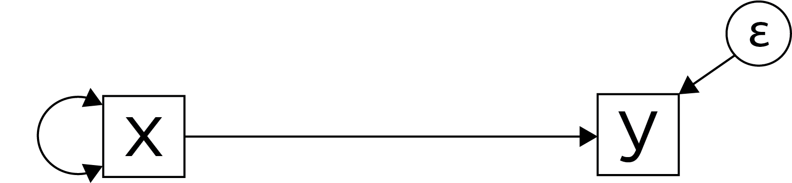
Figure 7.1 depicts a path analyis diagram of a bivariate regression model of one variable, \(x\), predicting another variable, \(y\). The two-headed arrow into \(x\) depicts the variance of \(x\). That is, the variance of a variable conceptually represents the covariance of a variable with itself. Epsilon (\(\varepsilon\)) depicts the disturbance term for \(y\), capturing the portion of variance in \(y\) that is not accounted for by \(x\).
Figure 7.1: Path Analysis Diagram of a Bivariate Regression Model. The two-headed arrow into \(x\) depicts the variance of \(x\). Epsilon (\(\varepsilon\)) depicts the disturbance term for \(y\) (i.e., the variance in \(y\) that is not accounted for by \(x\)).
\(x\) is an exogenous variable, which means that it is not caused by another variable in the model. Thus, we know the variance of \(x\) (because it is not influenced by any other variable in the model). However, the variable \(y\) is endogenous—it is influenced by another variable in the model (in this case, \(x\) and \(\varepsilon\)). Using the path diagram, we can thus estimate the (model-implied) covariance between \(x\) and \(y\), the variance of \(y\), and the disturbance for \(y\) (\(\varepsilon\)). According to path tracing rules (described in Section 4.1), the model-implied covariance between \(x\) and \(y\) is in Equation 7.1:
\[
\text{Cov}(x,y) = \text{unstandardized path coefficient of } x \text{ on } y \times \text{Var}(x)
\tag{7.1}\]
There is one route that connects \(x\) to \(y\): backward from \(y\) to \(x\) to itself via the two-headed arrow representing the variable’s variance. The model-implied correlation (i.e., standardized covariance) between \(x\) and \(y\) is equal to the standardized path coefficient of \(x\) on \(y\), as in Equation 7.2:
\[
\small
\begin{aligned}
\text{Cor}(x,y) &= \text{standardized path coefficient of } x \text{ on } y \times \text{standardized Var}(x) \\
&= \text{standardized path coefficient of } x \text{ on } y \times 1 \\
&= \text{standardized path coefficient of } x \text{ on } y
\end{aligned}
\tag{7.2}\]
The model-implied variance of \(y\) is in Equation 7.3:
\[
\scriptsize
\begin{aligned}
\text{Var}(y) &= \text{unstandardized path coefficient of } x \text{ on } y \times \text{Var}(x) \times \text{unstandardized path coefficient of } x \text{ on } y + \text{disturbance} \\
&= (\text{unstandardized path coefficient of } x \text{ on } y)^2 \times \text{Var}(x) + \text{disturbance}
\end{aligned}
\tag{7.3}\]
There are two routes to (i.e., independent sources of variance in) \(y\):
one route goes backward from \(y\) to \(x\) to itself (via the two-headed arrow representing the variable’s variance) and then forward to \(y\).
another route goes from the disturbance term (\(\varepsilon\)) to \(y\)
The model-implied variance of the disturbance of \(y\) (\(\varepsilon\)) is in Equation 7.4:
The model-implied standardized variance of the disturbance of \(y\) (\(\varepsilon\)) is in Equation 7.5:
\[
\text{standardized Var}(\varepsilon) = 1 - (\text{standardized path coefficient of } x \text{ on } y)^2
\tag{7.5}\]
7.3.2 Components of a Structural Equation Model
7.3.2.1 Measurement Model
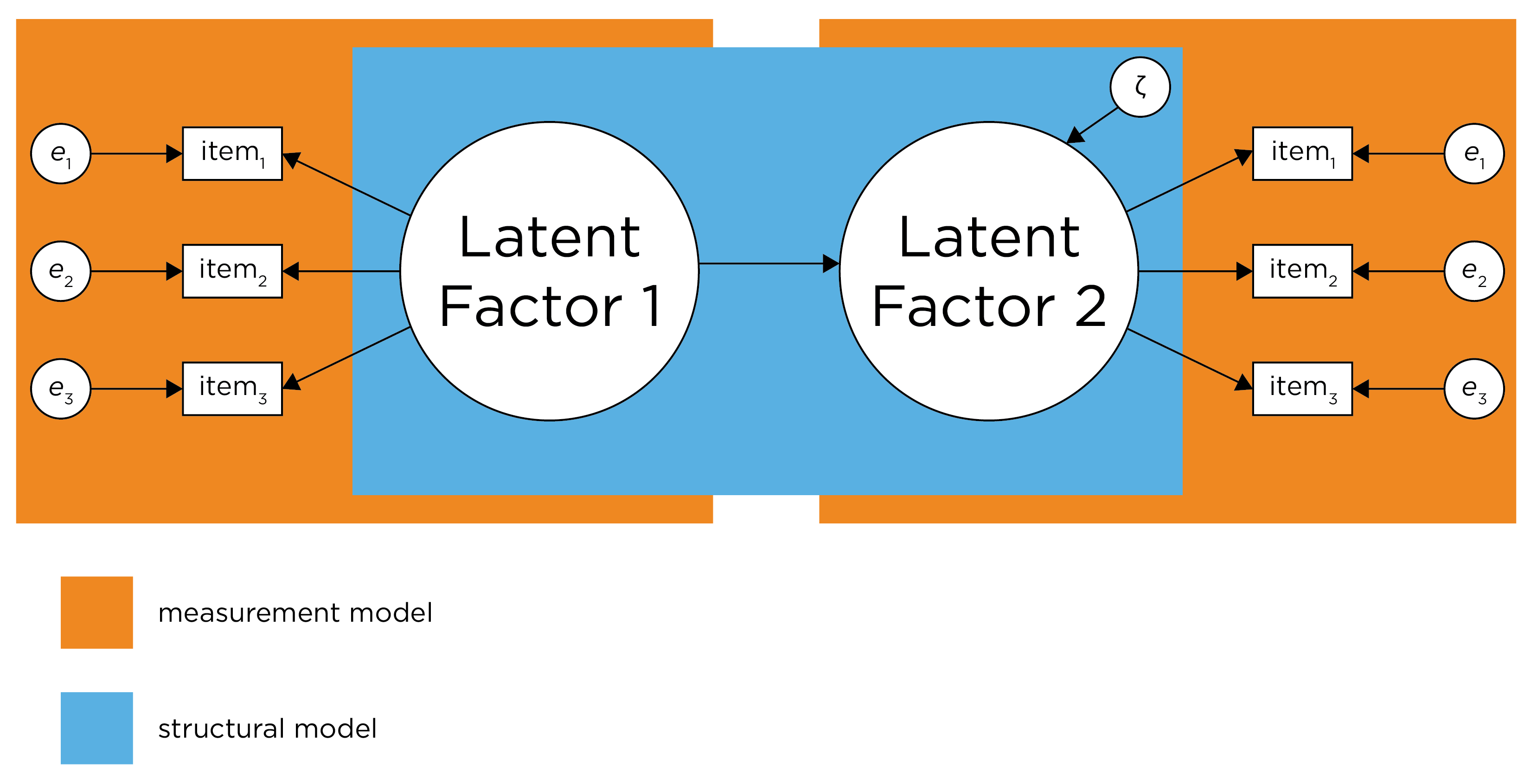
The measurement model is a crucial sub-component of any SEM model. A SEM model consists of two components: a measurement model and a structural model. The measurement model is a confirmatory factor analysis (CFA) model that identifies how many latent factors are estimated, and which items load onto which latent factor. The measurement model can also specify correlated residuals. Basically, the measurement model specifies your best understanding of the structure of the latent construct(s) given how they were assessed. Before fitting the structural component of a SEM, it is important to have a well-fitting measurement model for each construct in the model. In Section 7.3.2.1, I present an example of a measurement model.
7.3.2.2 Structural Model
The structural component of a SEM model includes the regression paths that specify the hypothesized causal relations among the latent variables. The disturbance (error term) for endogenous latent factors (i.e., latent factors that are predicted by other predictors) in the structural model is called zeta (\(\zeta\)).
SEM is CFA, but it adds regression paths that specify hypothesized causal relations between the latent variables, which is called the structural component of the model. The structural model includes the hypothesized causal relations between latent variables. A SEM model includes both the measurement model and the structural modelsee 7.2. SEM fits a model to observed data, or the variance-covariance matrix, and evaluates the degree of model misfit. That is, fit indices evaluate how likely it is that a given model gave rise to the observed data. In Section 7.11, I present an example of a SEM model.
Figure 7.2: Demarcation Between Measurement Model and Structural Model. Disturbance term is zeta. (Figure adapted from Civelek (2018), Figure 1, p. 7. Civelek, M. E. (2018). Essentials of structural equation modeling. Zea E-Books. https://doi.org/10.13014/K2SJ1HR5)
SEM is flexible in allowing you to specify measurement error and correlated errors. Thus, you do not need the same assumptions as in classical test theory, which assumes that errors are random and uncorrelated. But the flexibility of SEM also poses challenges because you must explicitly decide what to include—and not include—in your model. This flexibility can be both a blessing and a curse. If the model fit is unacceptable, you can try fitting a different model to see which fits better. Nevertheless, it is important to use theory as a guide when specifying and comparing competing models, and not just rely solely on model fit comparison. For example, the model you fit should depend on how you conceptualize each construct: as reflective or formative.
7.4 Estimating Latent Factors
7.4.1 Model Identification
7.4.1.1 Types of Model Identification
There are important practical issues to consider with both reflective and formative models. An important practical issue is model identification—adding enough constraints so that there is only one, best answer. The model is identified when each of the estimated parameters has a unique solution. For ensuring the model is identifiable, see the criteria for identification of the measurement and structural model here (archived at https://perma.cc/5C9E-LBWM).
Degrees of freedom in a SEM model is the number of known values minus the number of estimated parameters. The number of known values in a SEM model is the number of variances and covariances in the variance-covariance matrix of the manifest (observed) variables in addition to the number of means (i.e., the number of manifest variables), which can be calculated as: \(\frac{m(m + 1)}{2} + m\), where \(m = \text{the number of manifest variables}\). You can never estimate more parameters than the number of known values. A model with zero degrees of freedom is considered “saturated”—it will have perfect fit because the model estimates as many parameters as there are known values. All things equal (i.e., in terms of model fit with the same number of manifest variables), a model with more degrees of freedom is preferred for its parsimony, because fewer parameters are estimated.
Based on the number of known values compared to the number of estimated parameters, a model can be considered either just identified, under-identified, or over-identified. A just identified model is a model in which the number of known values is equal to the number of parameters to be estimated (degrees of freedom = 0). An under-identified model is a model in which the number of known values is less than the number of parameters to be estimated (degrees of freedom < 0). An over-identified model is a model in which the number of known values is greater than the number of parameters to be estimated (degrees of freedom > 0).
As an example, there are 14 known values for a model with 4 manifest variables (\(\frac{4(4 + 1)}{2} + 4 = 14\)): 4 variances, 6 covariances, and 4 means.
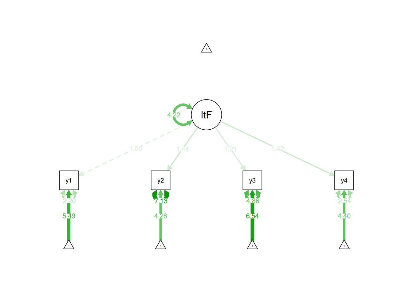
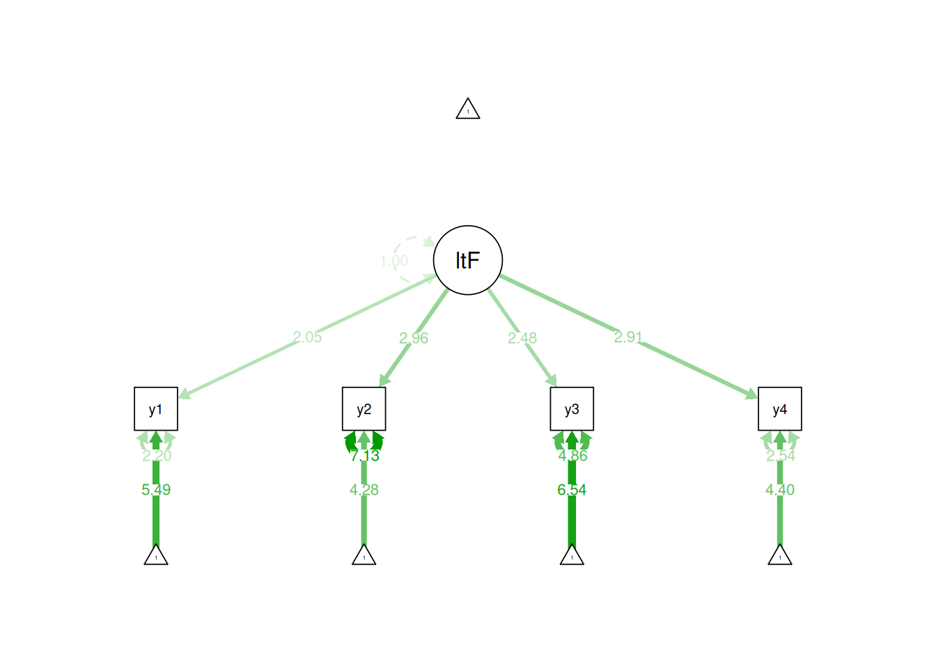
In the marker variable method, one of the indicators (i.e., manifest variables) is set to have a loading of 1. Here are examples of using the marker variable method for identification of a latent variable:
Figure 7.3: Identifying a Latent Variable Using the Marker Variable Approach.
7.4.1.2.2 Effects Coding Method
In the effects coding method, the average of the factor loadings is set to be 1. The effects coding method is useful if you are interested in the means or variances of the latent factor, because the metric of the latent factor is on the metric of the indicators. Here are examples of using the effects coding method for identification of a latent variable:
Figure 7.4: Identifying a Latent Variable Using the Effects Coding Approach.
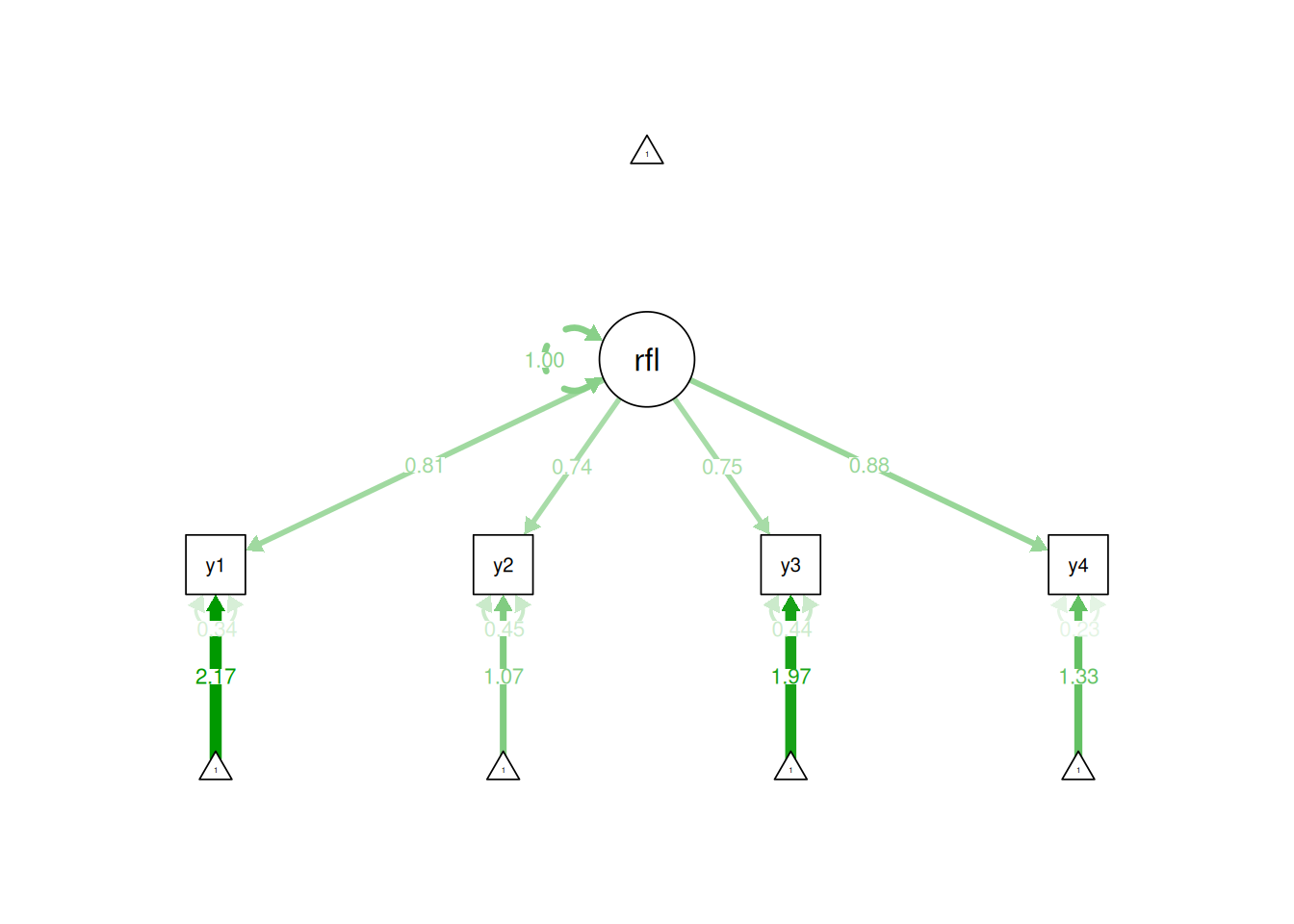
7.4.1.2.3 Standardized Latent Factor Method
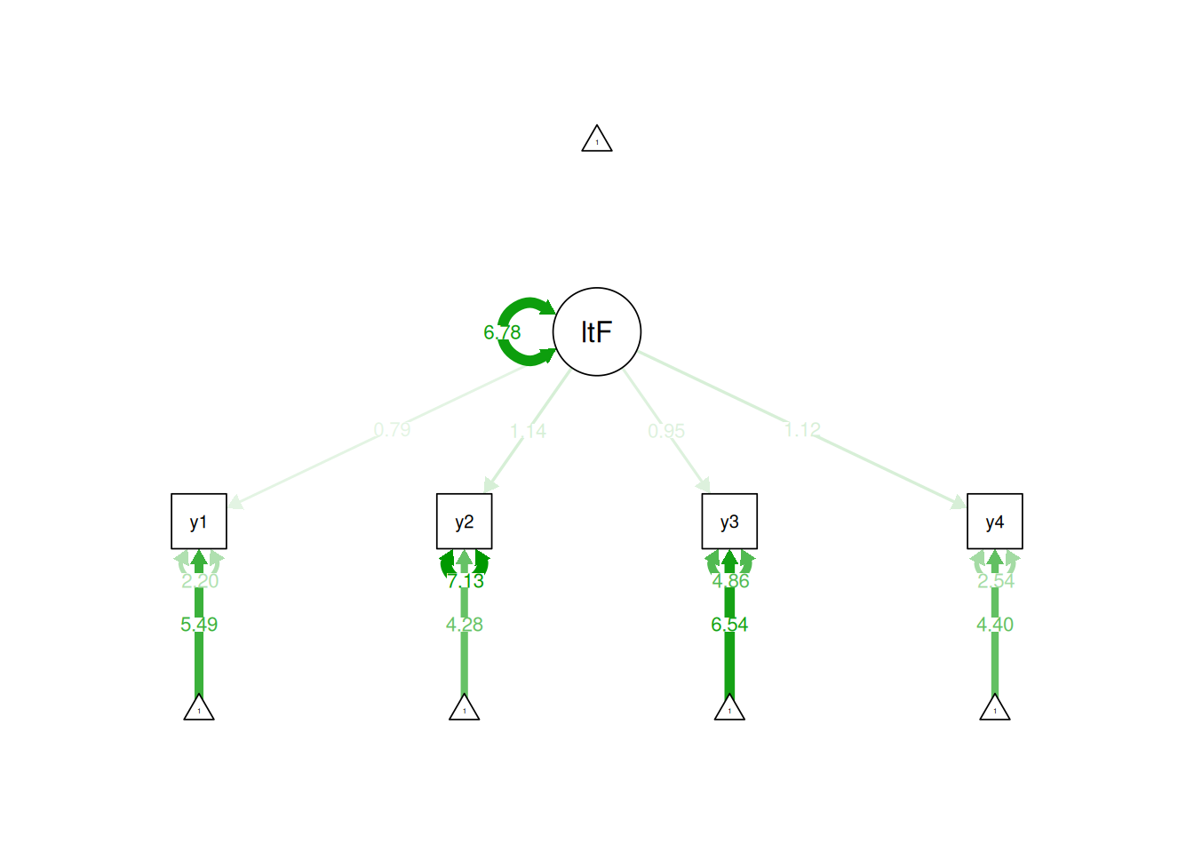
In the standardized latent factor method, the latent factor is set to have a mean of 0 and a standard deviation of 1. The standardized latent factor method is a useful approach if you are not interested in the means or variances of the latent factors and want to freely estimate the factor loadings. Here are examples of using the standardized latent factor method for identification of a latent variable:
Figure 7.5: Identifying a Latent Variable Using the Standardized Latent Factor Approach.
7.4.2 Types of Latent Factors
7.4.2.1 Reflective Latent Factors
For a reflective model with 4 indicators, we would need to estimate 12 parameters: a factor loading, error term, and intercept for each of the 4 indicators. Here are the parameters estimated:
Thus, for a reflective model, we only have to estimate a small number of parameters to specify what is happening in our model, so the model is parsimonious. With 4 indicators, the number of known values (14) is greater than the number of parameters (12). We have 2 degrees of freedom (\(14 - 12 = 2\)). Because the degrees of freedom is greater than 0, it is easy to identify the model—the model is over-identified. A reflective model with 3 indicators would have 9 known values (\(\frac{3(3 + 1)}{2} + 3 = 9\)), 9 parameters (3 factor loadings, 3 error terms, 3 intercepts), and 0 degrees of freedom, and it would be identifiable because it would be just-identified.
7.4.2.2 Formative Latent Factors
However, for a formative model, we must specify more parameters: a factor loading, intercept, and variance for each of the 4 indicators, all 6 permissive correlations, and 1 error term for the latent variable, for a total of 19 parameters. Here are the parameters estimated:
PT <-lavaanify( formativeModel_syntax,fixed.x =TRUE, # sem() sets fixed.x = TRUE by defaultmeanstructure =TRUE# estimator = "MLR" and missing = "ML" both set meanstructure = TRUE )lav_partable_df(PT)
[1] 0
Code
formativeModelFit
lavaan 0.6-21 ended normally after 7 iterations

  Estimator                                         ML
  Optimization method                           NLMINB
  Number of model parameters                         7

  Number of observations                            75
  Number of missing patterns                        10

Model Test User Model:

  Test statistic                                    NA
  Degrees of freedom                                -3
  P-value (Unknown)                                 NA

  Test statistic                                    NA
  Degrees of freedom                                -3
  P-value (Unknown)                                 NA
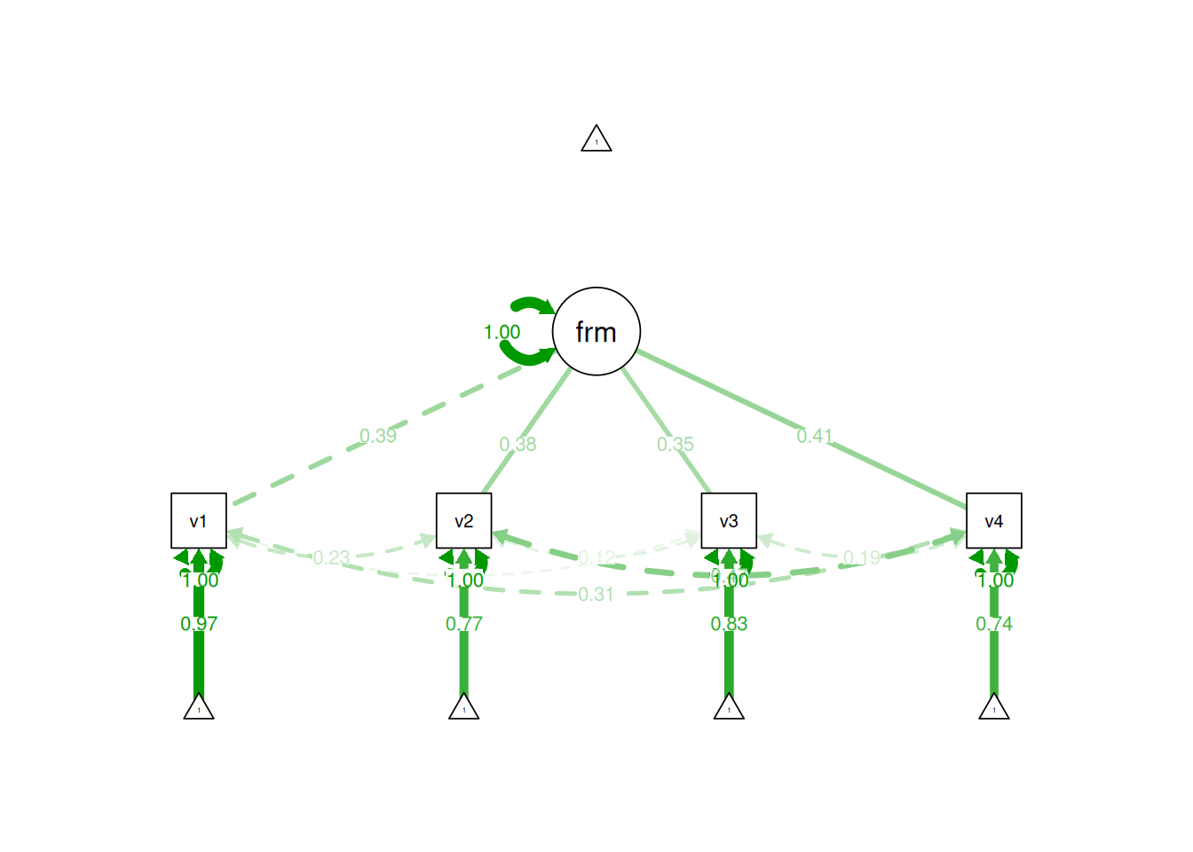
Figure 7.7: Example of an Under-Identified Formative Model.
For a formative model with 4 measures, the number of known values (14) is less than the number of parameters (19). The number of degrees of freedom is negative (\(14 - 19 = -5\)), thus the model is not able to be identified—the model is under-identified.
Thus, for a formative model, we need more parameters than we have data—the model is under-identified. Therefore, to estimate a formative model with 4 indicators, we must add assumptions and other variables that are consequences of the formative construct. Options for identifying a formative construct are described by Treiblmaier et al. (2011). See below for an example formative model that is identified because of additional assumptions.
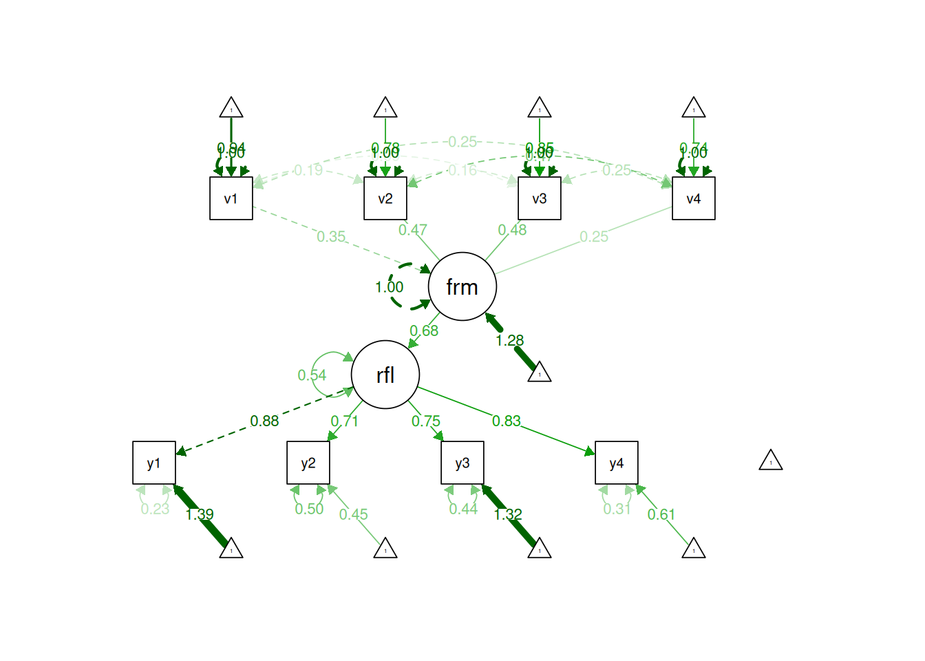
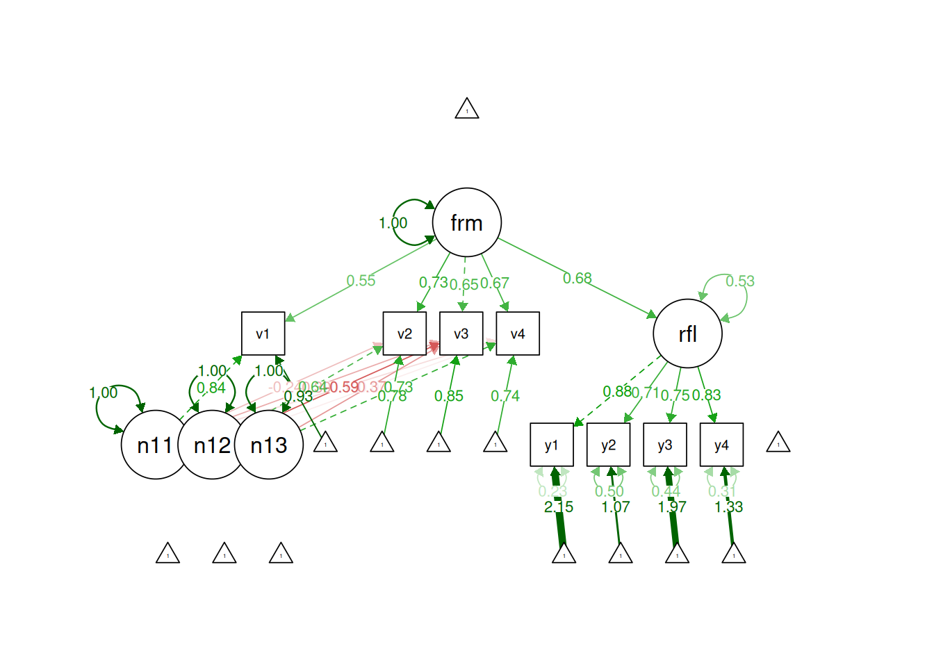
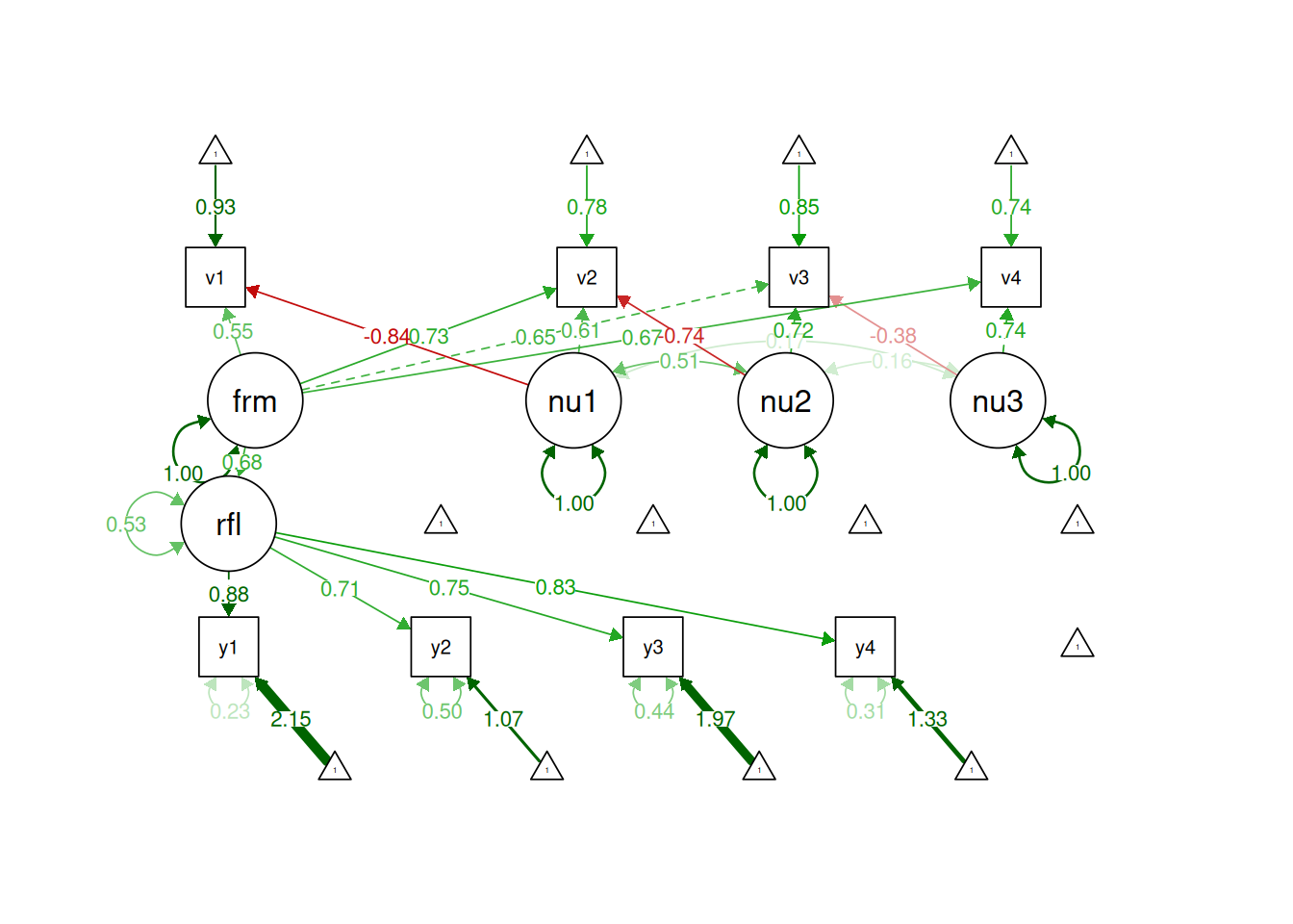
Figure 7.9: Example of an Identified Formative Model.
Thus, formative constructs are challenging to use in a SEM framework. To estimate a formative construct in a SEM framework, the formative construct must be used in the context of a model that allows some constraints. A formative latent factor includes a disturbance term, and is thus not entirely determined by the causal indicators (Bollen & Bauldry, 2011). A composite (such as in principal component analysis), by contrast, has no disturbance term and is therefore completely determined by the composite indicators (Bollen & Bauldry, 2011). Emerging techniques such as confirmatory composite analysis allow estimation of formative composites (Schamberger et al., 2023; Schuberth, 2023; Yu et al., 2023). Composites are a way to study part–whole relations such that the construct is made up of its indicators (Henseler, 2021); for example, a neural network is made up of neurons.
formativeModel3_syntax <-' # Specification of the reflective latent factor reflective =~ y1 + y2 + y3 + y4 # Specification of the associations between the observed variables v1 - v4 # and the emergent variable "formative" in terms of composite loadings. formative =~ NA*v1 + l11*v1+ l21*v2 + 1*v3 + l41*v4 # Label the variance of the formative composite formative ~~ varformative*formative # Specification of the associations between the observed variables v1 - v4 # and their excrescent variables in terms of composite loadings. nu11 =~ 1*v1 + l22*v2 + l32*v3 + l42*v4 nu12 =~ 0*v1 + 1*v2 + l33*v3 + l43*v4 nu13 =~ 0*v1 + 0*v2 + l34*v3 + 1*v4 # Label the variances of the excrescent variables nu11 ~~ varnu11*nu11 nu12 ~~ varnu12*nu12 nu13 ~~ varnu13*nu13 # Specify the effect of formative on reflective reflective ~ formative # The H-O specification assumes that the excrescent variables are uncorrelated. # Therefore, the covariance between the excrescent variables is fixed to 0: nu11 ~~ 0*nu12 + 0*nu13 nu12 ~~ 0*nu13 # Moreover, the H-O specification assumes that the excrescent variables are uncorrelated # with the emergent and latent variables. Therefore, the covariances between # the emergent and the excrescent varibales are fixed to 0: formative ~~ 0*nu11 + 0*nu12 + 0*nu13 reflective =~ 0*nu11 + 0*nu12 + 0*nu13 # In lavaan, the =~ command is originally used to specify a common factor model, # which assumes that each observed variable is affected by a random measurement error. # It is assumed that the observed variables forming composites are free from # random measurement error. Therefore, the variances of the random measurement errors # originally attached to the observed variables by the common factor model are fixed to 0: v1 ~~ 0*v1 v2 ~~ 0*v2 v3 ~~ 0*v3 v4 ~~ 0*v4 # Calculate the unstandardized weights to form the formative latent variable w1 := (-l32 + l22*l33 + l34*l42 - l22*l34*l43)/(1 - l11*l32 - l21*l33 + l11*l22*l33 - l34*l41 + l11*l34*l42 + l21* l34* l43 - l11* l22* l34* l43) w2 := (-l33 + l34*l43)/(1 - l11*l32 - l21*l33 + l11*l22*l33 - l34*l41 + l11*l34*l42 + l21*l34*l43 - l11*l22*l34*l43) w3 := 1/(1 - l11*l32 - l21*l33 + l11*l22*l33 - l34*l41 + l11*l34*l42 + l21*l34*l43 - l11*l22*l34*l43) w4 := -l34/(1 - l11*l32 - l21*l33 + l11*l22*l33 - l34*l41 + l11*l34*l42 + l21*l34*l43 - l11*l22*l34*l43) # Calculate the variances varv1 := l11^2*varformative + varnu11 varv2 := l21^2*varformative + l22^2*varnu11 + varnu12 varv3 := varformative + l32^2*varnu11 + l33^2*varnu12 + l34^2*varnu13 varv4 := l41^2*varformative + l42^2*varnu11 + l43^2*varnu12 + varnu13 # Calculate the standardized weights to form the formative latent variable w1std := w1*(varv1/varformative)^(1/2) w2std := w2*(varv2/varformative)^(1/2) w3std := w3*(varv3/varformative)^(1/2) w4std := w4*(varv4/varformative)^(1/2)'formativeModel3Fit <-sem( formativeModel3_syntax,data = PoliticalDemocracy,missing ="ML",estimator ="MLR")formativeModel3Parameters <-parameterEstimates(formativeModel3Fit)formativeModel3Parameters
You can generate the weights for the indicators (to be used in the model syntax) for the refined Henseler-Ogasawara specification using the following code:
Code
library("calculus")# First, construct the loading matrixloadingMatrix <-matrix(c('l11','l21',1,'l41','l12',1,0,0,0,'l23',1,0,0,0,'l34',1),4,4)# Check the structureloadingMatrix# Invert matrix, the first row contains the (unstandardized) weights# these can be copy and pasted to the lavaan model to specify the weights as new parametersmxinv(loadingMatrix)
Up to this point, we have discussed SEM with dimensional constructs. It also worth knowing about additional types of SEM models, including latent class models and mixture models, that handle categorical constructs. However, most disorders are more accurately conceptualized as dimensional than as categorical (Markon et al., 2011), so just because you can estimate categorical latent factors does not necessarily mean that one should.
7.5.1 Latent Class Models
In latent class models, the construct is not dimensional, but rather categorical. The categorical constructs are latent classifications and are called latent classes. For instance, the construct could be a diagnosis that influences scores on the measures. Latent class models examine qualitative differences in kind, rather than quantitative differences in degree.
7.5.2 Mixture Models
Mixture models allow for a combination of latent categorical constructs (classes) and latent dimensional constructs. That is, it allows for both qualitative and quantitative differences. However, this additional model complexity also necessitates a larger sample size for estimation. SEM generally requires a 3-digit sample size (\(N = 100+\)), whereas mixture models typically require a 4- or 5-digit sample size (\(N = 1,000+\)).
7.5.3 Exploratory Structural Equation Models
We describe exploratory structural equation models in Section 14.1.4.3.3.
7.6 Causal Diagrams: Directed Acyclic Graphs
A key tool when designing a structural equation model is a conceptual depiction of the hypothesized causal processes. A causal diagram depicts the hypothesized causal processes that link two or more variables. A common form of causal diagrams is the directed acyclic graph (DAG). DAGs provide a helpful tool to communicate about causal questions and help identify how to avoid bias (i.e., over-estimation) in associations between variables due to confounding (i.e., common causes) (Digitale et al., 2022). Free tools to create DAGs include the R package dagitty(Textor et al., 2017) and the associated browser-based extension, DAGitty: https://dagitty.net (archived at https://perma.cc/U9BY-VZE2). Path analytic diagrams (i.e., causal diagrams with boxes, circles, and lines) are described in Section 4.1.1 of Chapter 4. Karch (2025) provides a tool to create lavaanR syntax from a path analytic diagram: https://lavaangui.org.
7.7 Model Fit Indices
Various model fit indices can be used for evaluating how well a model fits the data and for comparing the fit of two competing models. Fit indices known as absolute fit indices compare whether the model fits better than the best-possible fitting model (i.e., a saturated model). Examples of absolute fit indices include the chi-square test, root mean square error of approximation (RMSEA), and the standardized root mean square residual (SRMR).
The chi-square test evaluates whether the model has a significant degree of misfit relative to the best-possible fitting model (a saturated model that fits as many parameters as possible; i.e., as many parameters as there are degrees of freedom); the null hypothesis of a chi-square test is that there is no difference between the predicted data (i.e., the data that would be observed if the model were true) and the observed data. Thus, a non-significant chi-square test indicates good model fit. However, because the null hypothesis of the chi-square test is that the model-implied covariance matrix is exactly equal to the observed covariance matrix (i.e., a model of perfect fit), this may be an unrealistic comparison. Models are simplifications of reality, and our models are virtually never expected to be a perfect description of reality. Thus, we would say a model is “useful” and partially validated if “it helps us to understand the relation between variables and does a ‘reasonable’ job of matching the data…A perfect fit may be an inappropriate standard, and a high chi-square estimate may indicate what we already know—that the hypothesized model holds approximately, not perfectly.” (Bollen, 1989, p. 268). The power of the chi-square test depends on sample size, and a large sample will likely detect small differences as significantly worse than the best-possible fitting model (Bollen, 1989).
RMSEA is an index of absolute fit. Lower values indicate better fit.
SRMR is an index of absolute fit with no penalty for model complexity. Lower values indicate better fit.
There are also various fit indices known as incremental, comparative, or relative fit indices that compare whether the model fits better than the worst-possible fitting model (i.e., a “baseline” or “null” model). Incremental fit indices include a chi-square difference test, the comparative fit index (CFI), and the Tucker-Lewis index (TLI). Unlike the chi-square test comparing the model to the best-possible fitting model, a significant chi-square test of the relative fit index indicates better fit—i.e., that the model fits better than the worst-possible fitting model.
CFI is another relative fit index that compares the model to the worst-possible fitting model. Higher values indicate better fit.
TLI is another relative fit index. Higher values indicate better fit.
Parsimony fit include fit indices that use information criteria fit indices, including the Akaike Information Criterion (AIC) and the Bayesian Information Criterion (BIC). BIC penalizes model complexity more so than AIC. Lower AIC and BIC values indicate better fit.
Chi-square difference tests and CFI can be used to compare two nested models. AIC and BIC can be used to compare two non-nested models.
Criteria for acceptable fit and good fit of SEM models are in Table 7.1. In addition, dynamic fit indexes have been proposed based on simulation to identify fit index cutoffs that are tailored to the characteristics of the specific model and data (McNeish, 2026; McNeish & Wolf, 2023); dynamic fit indexes are available via the dynamic package in R or with a webapp.
Table 7.1: Criteria for Acceptable and Good Fit of Structural Equation Models Based on Fit Indices.
SEM Fit Index
Acceptable Fit
Good Fit
RMSEA
\(\leq\) .08
\(\leq\) .05
CFI
\(\geq\) .90
\(\geq\) .95
TLI
\(\geq\) .90
\(\geq\) .95
SRMR
\(\leq\) .10
\(\leq\) .08
However, good model fit does not necessarily indicate a true model.
In addition to global fit indices, it can also be helpful to examine evidence of local fit (Kline, 2023; McNeish, 2026), such as the residual covariance matrix. The residual covariance matrix represents the difference between the observed covariance matrix and the model-implied covariance matrix (the observed covariance matrix minus the model-implied covariance matrix). These difference values are called covariance residuals. Standardizing the covariance matrix by converting each to a correlation matrix can be helpful for interpreting the magnitude of any local misfit. This is known as a residual correlation matrix, which is composed of correlation residuals. Correlation residuals greater than |.10| are possible evidence for poor local fit (Kline, 2023). If a correlation residual is positive, it suggests that the model underpredicts the observed association between the two variables (i.e., the observed covariance is greater than the model-implied covariance). If a correlation residual is negative, it suggests that the model overpredicts their observed association between the two variables (i.e., the observed covariance is smaller than the model-implied covariance). If the two variables are connected by only indirect pathways, it may be helpful to respecify the model with direct pathways between the two variables, such as a direct effect (i.e., regression path) or a covariance path. For guidance on evaluating local fit, see Kline (2024).
Correlation matrices of various types using the cor.table() function from the petersenlab package (Petersen, 2025) are in Tables 7.2, 7.3, and 7.4.
Code
cor.table(mydataSEM, dig =2)cor.table(mydataSEM, type ="manuscript", dig =2)cor.table(mydataSEM, type ="manuscriptBig", dig =2)
Table 7.2: Correlation Matrix with r, n, and p-values.
measure1
measure2
measure3
1. measure1.r
1.00
.54***
.68***
2. sig
NA
.00
.00
3. n
298
297
298
4. measure2.r
.54***
1.00
.78***
5. sig
.00
NA
.00
6. n
297
298
298
7. measure3.r
.68***
.78***
1.00
8. sig
.00
.00
NA
9. n
298
298
299
Table 7.3: Correlation Matrix with Asterisks for Significant Associations.
measure1
measure2
measure3
1. measure1
1.00
2. measure2
.54***
1.00
3. measure3
.68***
.78***
1.00
Table 7.4: Correlation Matrix.
measure1
measure2
measure3
1. measure1
1.00
2. measure2
.54
1.00
3. measure3
.68
.78
1.00
7.9 Measurement Model (of a Given Construct)
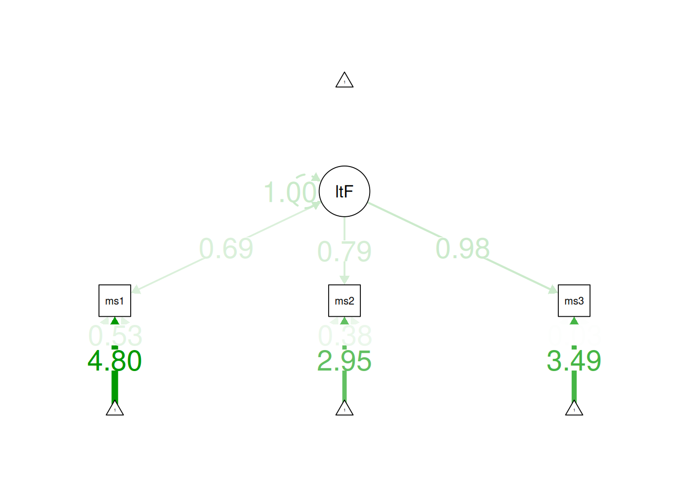
Even though CFA models are measurement models, I provide separate examples of a measurement model and CFA models in my examples because CFA is often used to test competing factor structures. For instance, you could use CFA to test whether the variance in several measures’ scores is best explained with one factor or two factors. In the measurement model below, I present a simple one-factor model with three measures. The measurement model is what we settle on as the estimation of each construct before we add the structural component to estimate the relations among latent variables. Basically, we add the structural component onto the measurement model. In Section 7.10, I present a CFA model with multiple latent factors.
This measurement model with three indicators is just-identified—the number of parameters estimated is equal to the number of known values, thus leaving 0 degrees of freedom. In the model, all three indicators load strongly on the latent factor (measure 1: \(\beta = 0.69\); measure 2: \(\beta = 0.79\); measure 3: \(\beta = 0.98\)). Thus, the loadings of this measurement model would be consistent with a reflective latent construct. In terms of interpretation, all three indicators loaded positively on the latent factor, so higher levels of the latent factor are indicated by higher levels on the indicators. However, one of the estimated observed variances is negative, so the model is not able to be estimated accurately. Thus, we would need to make additional adjustments in order to estimate the model.
$latentFactor

Composite `latentFactor` is composed of observed variables:
    measure1, measure2, measure3
True-score variance is represented by common factor(s):
    latentFactor
Total variance of composite `latentFactor` determined from the unrestricted model.
The proportion attributable to "true" scores is its model-based estimate of reliability ("omega"):

[1] 0.925
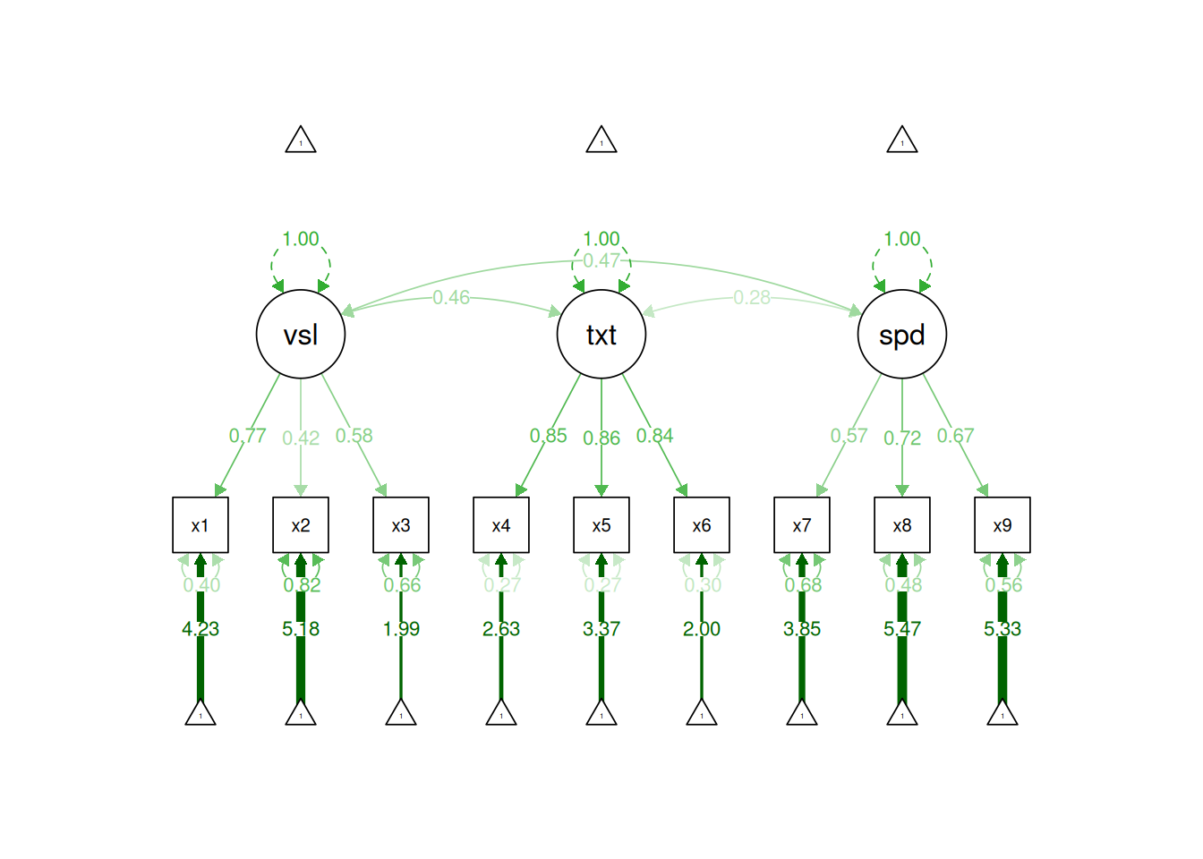
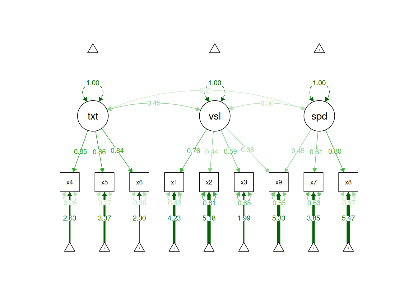
In this model, all nine indicators load strongly on their respective latent factor. Thus, this measurement model would be defensible. In terms of interpretation, all indicators load positively on their respective latent factor, so higher levels of the latent factor are indicated by higher levels on the indicators.
According to model fit estimates, the model fit is good according to SRMR and acceptable according to CFI, but the model fit is weaker according to RMSEA and TLI. Thus, we may want to consider adjustments to improve the model fit. In general, we want to make decisions regarding what parameters to estimate based on theory in conjunction with empiricism.
Modification indices indicate potential additional parameters that could be estimated and that would improve model fit. For instance, the modification indices in Table 7.5 (generated from the syntax below) indicate a few additional factor loadings (i.e., cross-loadings) or correlated residuals that could substantially improve model fit. However, it is generally not recommended to blindly estimate additional parameters solely based on modification indices. Rather, it is generally advised to consider modification indices in light of theory.
$visual

Composite `visual` is composed of observed variables:
    x1, x2, x3
True-score variance is represented by common factor(s):
    visual
Total variance of composite `visual` determined from the unrestricted model.
The proportion attributable to "true" scores is its model-based estimate of reliability ("omega"):

[1] 0.612

$textual

Composite `textual` is composed of observed variables:
    x4, x5, x6
True-score variance is represented by common factor(s):
    textual
Total variance of composite `textual` determined from the unrestricted model.
The proportion attributable to "true" scores is its model-based estimate of reliability ("omega"):

[1] 0.885

$speed

Composite `speed` is composed of observed variables:
    x7, x8, x9
True-score variance is represented by common factor(s):
    speed
Total variance of composite `speed` determined from the unrestricted model.
The proportion attributable to "true" scores is its model-based estimate of reliability ("omega"):

[1] 0.686
7.10.10 Modify Model Based on Modification Indices
In the model below, I modified the model based on estimating an additional factor loading (assuming the additional factor loading is theoretically supported). This could be supported, for instance, if a given test involves considerable skills in both the visual domain and in speed of processing. When the same indicator loads simultaneously on two factors, this is called a cross-loading. Cross-loadings can complicate the interpretation of latent factors, as discussed in Section 14.1.4.5 of the chapter on factor analysis.
After fitting the additional factor loading, the model fits well according to RMSEA, CFI, and SRMR, and the model fit is acceptable according to TLI. Thus, this model could be defensible.
The modified model with the cross-loading and the original model are considered “nested” models. The original model is nested within the modified model because the modified model includes all of the terms of the original model along with additional terms. To confirm that the models are nested, I use the net() function from the semTools package (Jorgensen et al., 2021).
Code
net(cfaModelFit, cfaModel2Fit)
        If cell [R, C] is TRUE, the model in row R is nested within column C.

        If the models also have the same degrees of freedom, they are equivalent.

        NA indicates the model in column C did not converge when fit to the
        implied means and covariance matrix from the model in row R.

        The hidden diagonal is TRUE because any model is equivalent to itself.
        The upper triangle is hidden because for models with the same degrees
        of freedom, cell [C, R] == cell [R, C].  For all models with different
        degrees of freedom, the upper diagonal is all FALSE because models with
        fewer degrees of freedom (i.e., more parameters) cannot be nested
        within models with more degrees of freedom (i.e., fewer parameters).

                       cfaModel2Fit cfaModelFit
cfaModel2Fit (df = 23)
cfaModelFit (df = 24)  TRUE
Model fit of nested models can be compared with a chi-square difference test.
Code
anova(cfaModelFit, cfaModel2Fit)
In this case, the model with the cross-loading fits significantly better (i.e., has a significantly smaller chi-square value) than the model without the cross-loading.
One can also compare nested models using a robust likelihood ratio test:
Model 1
 Class: lavaan
 Call: lavaan::lavaan(model = cfaModel2_syntax, data = HolzingerSwineford1939, ...

Model 2
 Class: lavaan
 Call: lavaan::lavaan(model = cfaModel_syntax, data = HolzingerSwineford1939, ...

Variance test
  H0: Model 1 and Model 2 are indistinguishable
  H1: Model 1 and Model 2 are distinguishable
    w2 = 0.120,   p = 0.00049

Robust likelihood ratio test of distinguishable models
  H0: Model 2 fits as well as Model 1
  H1: Model 1 fits better than Model 2
    LR = 32.923,   p = 8.11e-08
For non-nested models, one can compare model fit with AIC, BIC, or the Vuong test.
Model 1
 Class: lavaan
 Call: lavaan::lavaan(model = cfaModel_syntax, data = HolzingerSwineford1939, ...

Model 2
 Class: lavaan
 Call: lavaan::lavaan(model = cfaModel2_syntax, data = HolzingerSwineford1939, ...

Variance test
  H0: Model 1 and Model 2 are indistinguishable
  H1: Model 1 and Model 2 are distinguishable
    w2 = 0.120,   p = 0.00049

Non-nested likelihood ratio test
  H0: Model fits are equal for the focal population
  H1A: Model 1 fits better than Model 2
    z = -2.734,   p = 0.997
  H1B: Model 2 fits better than Model 1
    z = -2.734,   p = 0.003128
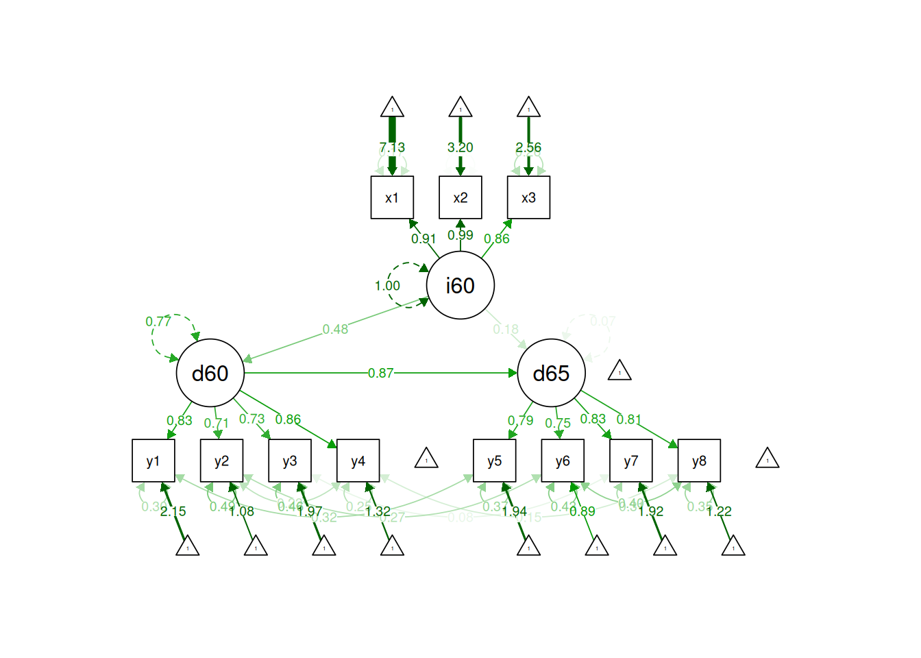
In this model, we fit a measurement model with three latent factors in addition to a structural model with regressions estimated among the latent factors.
Output from a SEM model includes information such as regression coefficients, intercepts, variances, and model fit indices. As noted above, there are two chi-square tests. In lavaan syntax, one is labeled “Model Test User Model” and the other is labeled “Model Test Baseline Model.” The chi-square test labeled “Model Test User Model” refers to the chi-square test of whether the model fits worse than the best-possible fitting model (the saturated model). In this case, the p-value of the robust chi-square test is \(0.17\). Thus, the model does not show significant misfit—i.e., the model does not fit significantly worse than the best-possible fitting model. The chi-square test labeled “Model Test Baseline Model” refers to the chi-square test of whether the model fits better than the worst-possible fitting model (the null model). In this case, the p-value of the robust chi-square test in comparison to the worse-possible fitting model is < .05. Thus, the model fits significantly better than the worst-possible-fitting model.
In terms of the model findings, ind60 was significantly positively associated with dem60, dem60 was significantly positively associated with dem65, and ind60 was marginally significantly positively associated with dem65.
$ind60

Composite `ind60` is composed of observed variables:
    x1, x2, x3
True-score variance is represented by common factor(s):
    ind60
Total variance of composite `ind60` determined from the unrestricted model.
The proportion attributable to "true" scores is its model-based estimate of reliability ("omega"):

[1] 0.938

$dem60

Composite `dem60` is composed of observed variables:
    y1, y2, y3, y4
True-score variance is represented by common factor(s):
    ind60
Total variance of composite `dem60` determined from the unrestricted model.
The proportion attributable to "true" scores is its model-based estimate of reliability ("omega"):

[1] 0.198

$dem65

Composite `dem65` is composed of observed variables:
    y5, y6, y7, y8
True-score variance is represented by common factor(s):
    ind60, dem60
Total variance of composite `dem65` determined from the unrestricted model.
The proportion attributable to "true" scores is its model-based estimate of reliability ("omega"):

[1] 0.786
There are many benefits of fitting a model in SEM (or in other latent variable approaches). First, unlike classical test theory, SEM can allow correlated errors. With SEM, you do not need to make as restrictive assumptions as in classical test theory. Second, unlike multiple regression, SEM can handle multiple dependent variables simultaneously. Third, SEM uses all available information (data) using a technique called full information maximum likelihood (FIML), even if participants have missing scores on some variables. By contrast, multiple regression and many other statistical analyses use listwise deletion, in which they discard participants if they have a missing score on any of the model variables. Fourth, whereas multiple regression assumes nonnormally distributed residuals, SEM can handle nonnormally distributed residuals via robust standard errors (i.e., MLR estimator) and robust fit indices. Fifth, SEM can estimate mediation in a single model.
Sixth, as described in the next section (Section 7.12.1), SEM can be used to account for different forms of measurement error (e.g., method bias). Accounting for measurement error allows disattenuating associations with other constructs. I provide an example showing that SEM disattenuates associations for measurement error in Section 5.6.3. All of these benefits allow SEM to generate purer estimation of constructs, more accurate estimates of people’s levels on constructs, and more accurate estimates of associations between constructs. Our theories deal with constructs (latent variables), not with fallible measurements of constructs (manifest variables). Thus, SEM allows for models that are better aligned with theory than other statistical approaches that do not account for measurement error.
A more practical utility of SEM is that it allows one to obtain “purer” estimates of latent constructs (and people’s standing on them) by discarding measurement error, and you do not have to assume all errors are uncorrelated!
7.13 Guidelines for Reporting Reliability and Validity in SEM
Guidelines for reporting reliability and validity in structural equation modeling are provided by Cheung et al. (2024).
I provide an example of how to conduct power analysis of an SEM model to determine the sample size needed to detect a hypothesized effect of a given effect size. To perform the power analysis, I use Monte Carlo simulation (Hancock & French, 2013; Muthén & Muthén, 2002). It is named after the Casino de Monte-Carlo in Monaco because Monte Carlo simulations involve random samples (random chance), as might be found in casino gambling. Monte Carlo simulations can be used to determine the sample size needed to detect a target parameter of a given effect size, using the following four steps (Wang & Rhemtulla, 2021):
Specify the sample size, a hypothesized true population SEM model, and all of its parameter values (e.g., factor loadings, intercepts, residuals, means, variances, covariances, regression paths, sample size);
Generate a large number (e.g., 1,000) of random samples based on the hypothesized model and population values specified;
Fit a SEM model to each of the generated samples, and for each one, record whether the target parameter is significantly different from zero;
Calculate power as the proportion of simulated samples that produce a statistically significant estimate of the target parameter.
These four steps can be repeated with different sample sizes to identify the sample size that is needed to have a particular level of power (e.g., .80).
Power analysis of structural equation models using Monte Carlo simulation was estimated using the simsem package (Pornprasertmanit et al., 2021). These examples were adapted from the simsem documentation:
The population model was used to generate the simulated data. It is important to specify each parameter value in the population model based on theory and/or prior empirical research, especially meta-analysis of the target population (when possible).
Specifying the expected distributions of the data variables is an optional step, but it can help give you more realistic estimates of your likely power, especially when the data are non-normally distributed. First, identify the order in which the indicator variables appear in the model, so you can know the order to specify skewness and kurtosis (which I specify in the next section):
Specify the skewness and kurtosis of the data variables. In this example, I set the variables \(x1\)–\(x3\) (the first three variables) to have skewness of 1.3 and kurtosis of 1.8, and I set the variables \(y1\)–\(y8\) (the next eight variables) to have a skewness of 2 and a kurtosis of 4.
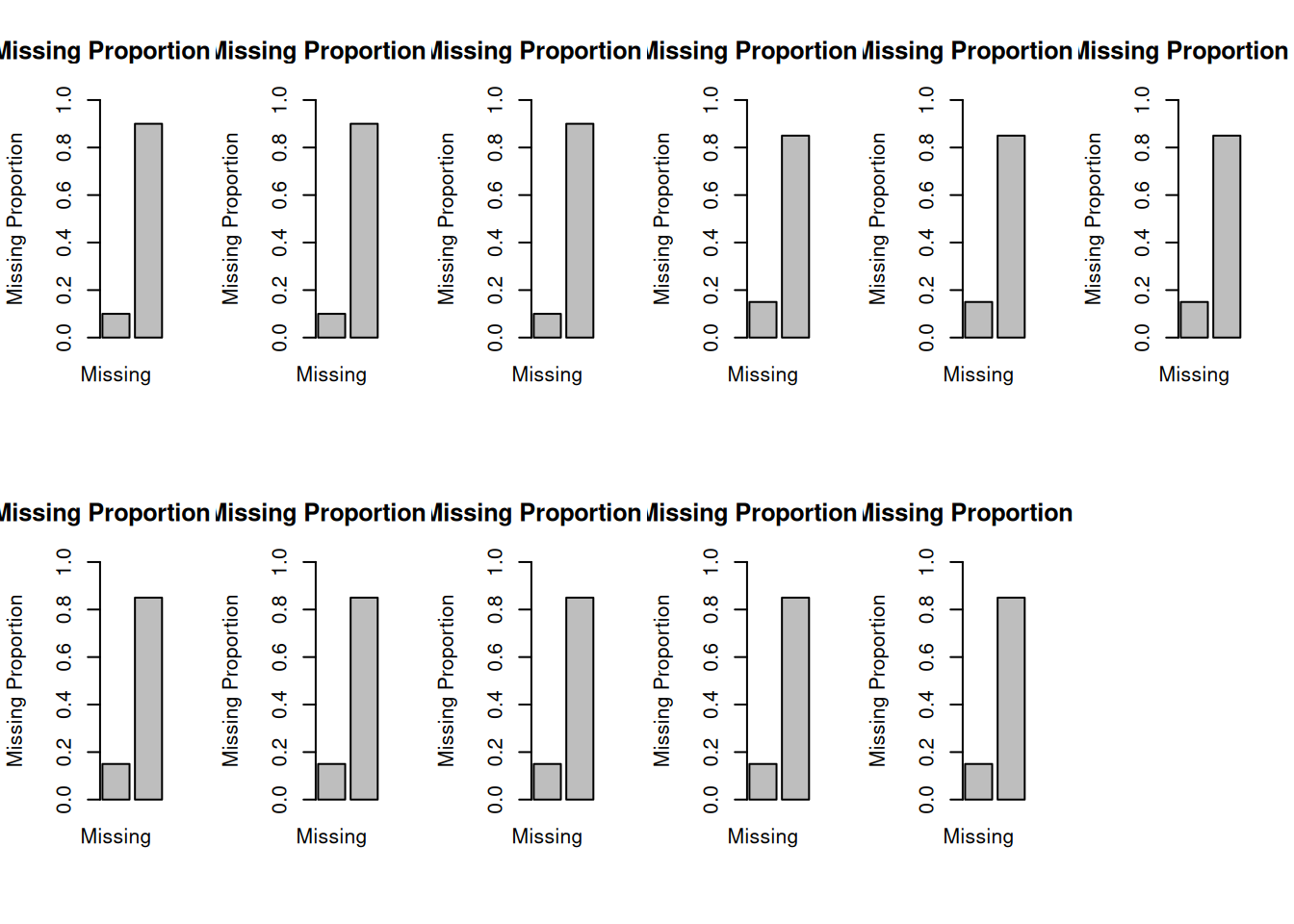
Specifying the extent and pattern of missingness is an optional step, but it can help give you more realistic estimates of your likely power, especially when there is extensive missing data and/or the data are not missing completely at random (MCAR). For an example of specifying the extent and pattern of missingness in the context of a Monte Carlo power analysis, see Beaujean (2014). In this example, I set 10% of values to be missing for variables \(x1\), \(x2\), and \(x3\). I set 15% of values to be missing for variables \(y1\)–\(y8\). I assumed the missingness mechanism to be MCAR. To set missingness to be missing at random (MAR), add a covariate in the missingness formula (see Beaujean, 2014). I set the model to use full information maximum likelihood (FIML) estimation to handle missingness. If you set \(m\) to a value greater than zero, it will allow use of multiple imputation instead of FIML. Statistical power with multiple imputation tends to be lower than with FIML unless the number of imputations is large (Graham et al., 2007).
Figure 7.14: Percent Missingness Specified for Each Variable.
7.14.5 Specify Sample Sizes and Repetitions
Specify the sample sizes to evaluate in the Monte Carlo simulation and the number of repetitions per sample size.
Code
sampleSizes <-150:700repetitionsPerSampleSize <-2
7.14.6 Monte Carlo Simulation to Generate Data from the Population Parameter Values
Conduct Monte Carlo simulation with \(2\) repetitions per sample size \((N\text{s} = 150–700)\). The multicore backend was used for parallel processing. Parallel processing distributes a larger computation task across multiple computing processes or cores, and runs them simultaneously (in parallel) to speed up execution time (if multiple processes or cores are available). If you choose to do processing in serial rather than parallel (by setting multicore = FALSE), you will need to run a special set.seed() command, prior to running the sim() command, to get reproducible results with those obtained from parallel processing: set.seed(seedNumber, "L'Ecuyer-CMRG"), where seedNumber is the value used for the seed. Warning: this code takes a while to run based on \(551\) different sample sizes \((700 - 150 + 1)\) and \(2\) repetitions per sample size, for a total of \(1102\) iterations \(([700 - 150 + 1]\) sample sizes \(\times\)\(2\) repetitions per sample size \(= 1102\) iterations). You can reduce the number of sample sizes and/or repetitions per sample size to be faster.
============ Wall Time ============
  1. Error Checking and setting up data-generation and analysis template:        0.001
  2. Set combinations of n, pmMCAR, and pmMAR:                                   0.001
  3. Setting up simulation conditions for each replication:                      0.018
  4. Total time elapsed running all replications:                             1157.756
  5. Combining outputs from different replications:                              0.072

============ Average Time in Each Replication ============
  1. Data Generation:                                  0.080
  2. Impose Missing Values:                            0.014
  3. User-defined Data-Transformation Function:        0.000
  4. Main Data Analysis:                               2.465
  5. Extracting Outputs:                               1.620

============ Summary ============
  Start Time:                   2026-07-10 03:59:40
  End Time:                     2026-07-10 04:18:58
  Wall (Actual) Time:             1157.848
  System (Processors) Time:       4606.244
  Units:                        seconds
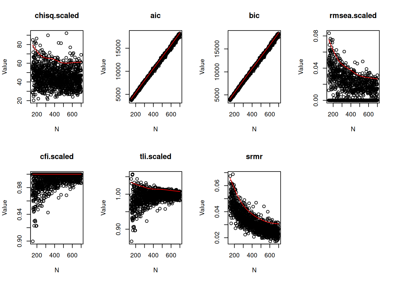
7.14.11 Cutoffs of Fit Indices
7.14.11.1 Plot of Cutoffs of Fit Indices
At \(\alpha = .05\)
Code
plotCutoff(output, alpha = .05)
Figure 7.15: Plot of Cutoffs of Fit Indices From Monte Carlo Power Analysis.
7.14.11.2 Cutoffs of Fit Indices at Particular Sample Size
At \(N = 200\), \(\alpha = .05\)
Code
getCutoff(output, alpha = .05, nVal =200)
7.14.12 Statistical Power
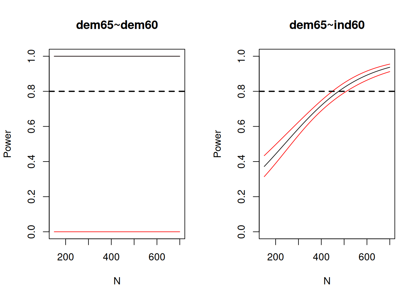
7.14.12.1 Plot of Power to Detect Various Parameters as a Function of Sample Size
At \(\alpha = .05\); dashed horizontal line represents power (\(1 - \beta\)) of .8
There are also SEM approaches for performing generalizability theory analyses. The reader is referred to examples by Vispoel et al. (2018), Vispoel et al. (2019), Vispoel et al. (2022), Vispoel et al. (2023), and Vispoel et al. (2024).
7.16 Conclusion
Structural equation modeling (SEM) is an advanced modeling approach that allows estimating latent variables as the common variance from multiple measures. SEM holds promise to account for measurement error and method biases, which allows one to get more accurate estimates of constructs, people’s standing on constructs (i.e., individual differences), and associations between constructs.
Note: Several of the following questions use data from the Children of the National Longitudinal Survey of Youth Survey (CNLSY). The CNLSY is a publicly available longitudinal data set provided by the Bureau of Labor Statistics (https://www.bls.gov/nls/nlsy79-children.htm#topical-guide; archived at https://perma.cc/EH38-HDRN). The CNLSY data file for these exercises is located on the book’s page of the Open Science Framework (https://osf.io/3pwza). Children’s behavior problems were rated in 1988 (time 1: T1) and then again in 1990 (time 2: T2) on the Behavior Problems Index (BPI). Below are the items corresponding to the Antisocial subscale of the BPI:
cheats or tells lies
bullies or is cruel/mean to others
does not seem to feel sorry after misbehaving
breaks things deliberately
is disobedient at school
has trouble getting along with teachers
has sudden changes in mood or feeling
Fit a confirmatory factor analysis model to the seven items of the Antisocial subscale of the Behavior Problems Index at T1. Set the first indicator to be the referent indicator (to set the scale of the latent factor) by setting its loading to one. Allow the factor loadings of the other indicators to be freely estimated. Set the mean (intercept) of the latent factor to be zero. Do not allow the residuals to be correlated. Use full information maximum likelihood (FIML) to account for missing data. Use robust standard errors to account for non-normally distributed data.
This is an over-simplification, but for now let us assume a model fits “well” if CFI \(\geq .95\), RMSEA \(< .08\), and SRMR \(< .08\)(Schreiber et al., 2006). Did the model fit well? What does this indicate?
Examine the modification indices. Which modification would result in the greatest improvement in model fit? Why do you think this modification would improve model fit?
Fit the modified confirmatory factor analysis model to make the suggested revision you identified in 1b.
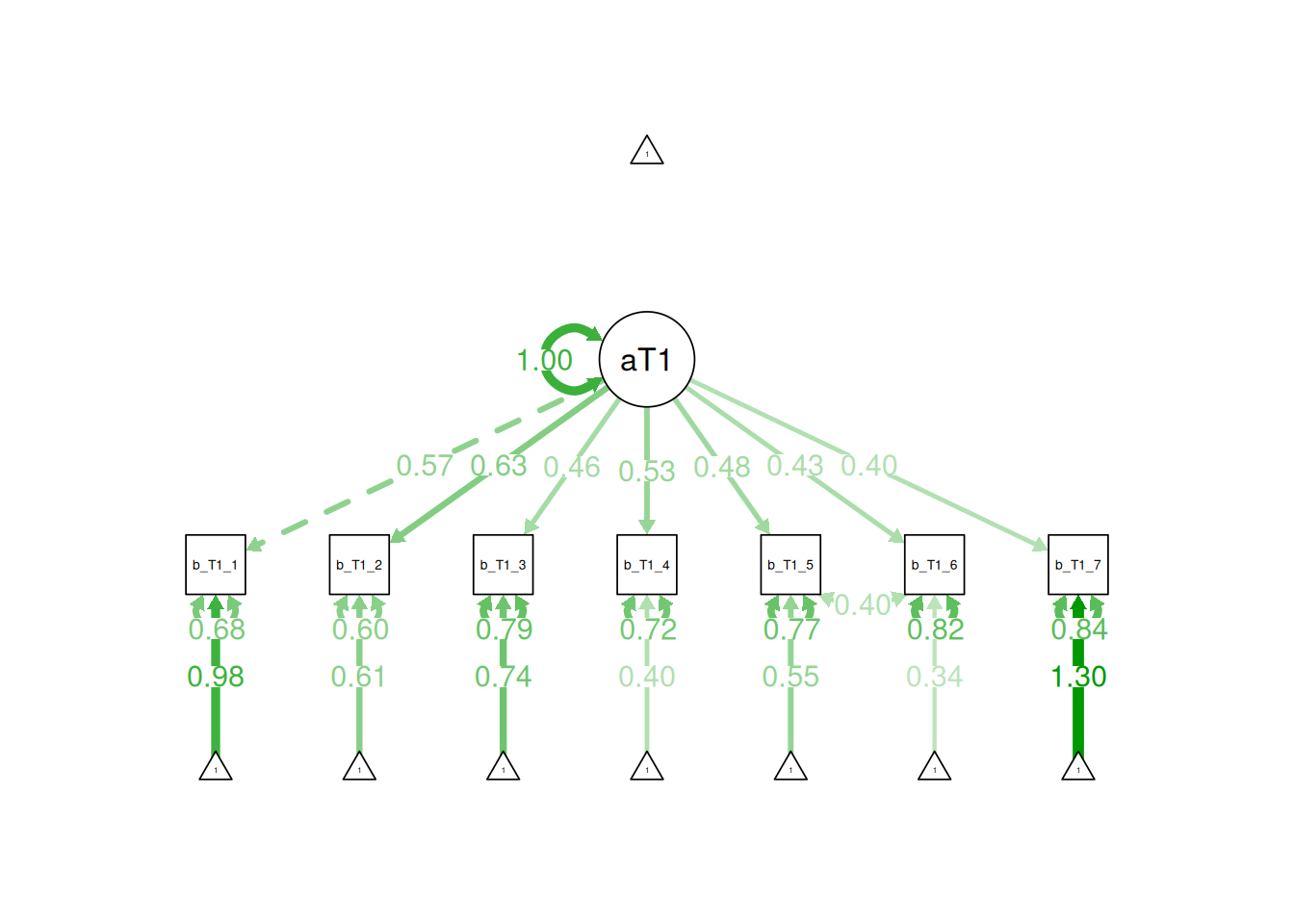
Provide a figure of the model with standardized coefficients.
The modified model and the original model are considered “nested” models. The original model is nested within the modified model because the modified model includes all of the terms of the original model along with additional terms. Model fit of nested models can be directly compared with a chi-square difference test. Did the modified model fit better than the original model?
Did the modified model fit well? What does this indicate? Which item is most strongly with the latent factor? Which item is most weakly associated with the latent factor?
What is the estimate of internal consistency reliability of the items, based on coefficient omega?
Fit a confirmatory factor analysis model to the seven items of the Antisocial subscale of the Behavior Problems Index at both T1 and T2 simultaneously in the same model. Allow the items at T1 to load onto a different factor than the items at T2 (i.e., a two-factor model—one antisocial at each time point). Set the scale of the latent factors by standardizing the latent factors—set their means to one and their variances to zero. This allows you to freely estimate the factor loadings of all items (instead of setting a reference indicator). Estimate the covariance between the two latent factors. Treat exogenous covariates as random variables (whose means, variances, and covariances are estimated) by specifying fixed.x = FALSE. Use full information maximum likelihood (FIML) to account for missing data. Use robust standard errors to account for non-normally distributed data. Apply the same modification you noted in 1b above to each factor.
Because the two latent factors are standardized, the “covariance” path between the two latent factors represents a correlation. What is the correlation between the latent factors? What is the correlation between the sum scores (bpi_antisocialT1Sum, bpi_antisocialT2Sum)? Which is greater and why?
Change the covariance path to a regression path from the latent factor at T1 predicting the latent factor at T2. Also include the sum score of anxious/depressed symptoms at T1 (bpi_anxiousDepressedSum) as a predictor of antisocial behavior at T2. Do anxious/depressed symptoms at T1 predict antisocial behavior at T2 controlling for prior levels of antisocial behavior at T1? Interpret the findings.
You plan to conduct a study that would examine whether stress and harsh parenting predict children’s antisocial behavior. Your hypothesis is that stress and harsh parenting both lead to children’s antisocial behavior. You would like to apply for a grant to test these hypotheses, but you first want to know what sample size you would need to have adequate power to detect the hypothesized effects. Because you read this book, you remember that measurement error attenuates the associations you would observe, which would make it less likely that you would be able to detect the true effect (if there truly is an effect). As a result, you plan to assess each construct with multiple measurement methods/measures. You plan to model each construct with a latent variable in a structural equation modeling framework to account for measurement error and disattenuate the associations, which will make the associations more closely approximate the true effect and will make it more likely that you will detect the effect if it exists. You plan to assess stress with three methods (self-report, friend report, cortisol), harsh parenting with four methods (parents’ self-report, spousal report, child report, observation), and children’s antisocial behavior with four methods (parent report, teacher report, child report, observation).
You conduct a power analysis with the following assumptions that you made based on theory and prior empirical research:
The factor loading for each measure on its latent variable is .75
Stress influences children’s antisocial behavior with a regression coefficient of .20
Harsh parenting influences children’s antisocial behavior with a regression coefficient of .45
Stress influences harsh parenting with a regression coefficient of .4
Set the intercepts of the indicators to zero. Set the scale of the latent factors by standardizing the latent factors—set their means to one and their variances to zero. Do not estimate correlated errors. You expect each measure to show 10% missingness, and for missingness to be completely at random (MCAR). Use full information maximum likelihood (FIML) to handle missing values. As is common with measures in clinical psychology, you expect each measure to be positively skewed with a skewness of 2.5 and leptokurtic with a kurtosis of 5. Use robust standard errors to account for non-normally distributed data. Using a seed of 52242, an alpha level of .05, and one repetition per sample size, in the simsem package:
What sample size would you need to have adequate power to detect the effect of stress on antisocial behavior and the effect of harsh parenting on antisocial behavior?
Due to financial and time constraints of the grant, you are only able to collect a sample size of 150. What power would you have to detect the effect of stress on antisocial behavior and the effect of harsh parenting on antisocial behavior?
Your study finds that neither stress nor harsh parenting predicts antisocial behavior. How would you interpret each of these findings?
Re-run the power analysis with normally distributed values (skewness \(= 0\), kurtosis \(= 0\)), using 50 repetitions with a sample size of 150. Did power to detect the hypothesized effects increase or decrease? What does this indicate?
7.18.2 Answers
The model did not fit well according to CFI \((0.88)\) and RMSEA \((0.09)\). SRMR \((0.05)\) was acceptable. The poor model fit indicates that it is unlikely that the causal process described by the hypothesized model gave rise to the observed data.
The modification that would result in the greatest model fit according to the modification indices is to allow indicators 5 and 6 to be correlated. These indicators reflect “disobedience at school” and “trouble getting along with teachers,” respectively. It is likely that allowing these two residuals to correlate would improve model fit because they both assess children’s behavior in the school context, and so they would continue to be associated with each other even after accounting for variance from the latent factor.
Figure 7.17: Figure of the Confirmatory Factor Analysis Model With Standardized Coefficients.
The modified model \((\chi^2[df = 13] = 33.68)\) fit significantly better than the original model \((\chi^2[df = 14] = 391.38)\) according to a chi-square difference test \((\Delta\chi^2[df = 1] = 833.51, p < .001)\).
The model fit well according to CFI \((0.9923114)\), RMSEA \((0.02416)\), and SRMR \((0.0133989)\). This indicates that there is evidence that one factor may do a good job of explaining the covariance among the indicators, especially when allowing the residuals of items 5 and 6 to correlate. The item that shows the strongest association with the latent factor is item 2 (“bullies or is cruel/mean to others”: standardized factor loading = \(.63\)). The item that shows the weakest association with the latent factor is item 7 (“sudden changes in mood or feeling”: standardized factor loading = \(.40\)). Thus, meanness seems more core to the construct of antisocial behavior compared to sudden mood changes.
The estimate of internal consistency reliability of items, based on coefficient omega (\(\omega\)), is \(.68\).
The correlation between the latent factor at T1 and T2 is \(\phi = .76\). The correlation between the sum score at T1 and T2 is \(r = .50\). This indicates that the correlation of individual differences across time (rank-order stability) is stronger for the latent factor than for the sum scores. This is likely because the latent factors account for measurement error whereas the sum scores do not, and associations are attenuated due to measurement error. Thus, the association of the latent factor at T1 and T2 likely more accurately reflects the “true” cross-time association of the construct (compared to the association of the sum scores at T1 and T2).
Yes, anxious/depressed symptoms significantly predicted antisocial behavior at T2 while controlling for prior levels of antisocial behavior \((B = 0.11, β = .11, SE = 0.02, p < .001)\). That is, anxious/depressed symptoms predicted relative (rank-order) changes in antisocial behavior from T1 to T2. This suggests that anxiety/depression may be a pathway to antisocial behavior for some children. Because the data come from an observational design, however, we cannot infer causality. For instance, the association could owe to the opposite direction of effect (antisocial behavior could lead to anxiety/depression) or to a third variable (e.g., victimization could lead to both antisocial behavior and anxiety/depression; i.e., antisocial behavior and anxiety/depression could share a common cause).
You would need a sample size of \(609\) to detect the effect of stress on children’s antisocial behavior. You would need a sample size of \(100\) to detect the effect of harsh parenting on children’s antisocial behavior.
You would have a power of \(.22\) to detect the effect of stress on children’s antisocial behavior. You would have a power of \(.91\) to detect the effect of harsh parenting on children’s antisocial behavior.
Because your study was well-powered to detect the effect of harsh parenting (\(\text{power} = .91\)) and you found no statistically significant association between harsh parenting and children’s antisocial behavior, it suggests that harsh parenting did not influence antisocial behavior in this sample (at least not with a large enough effect size to be practically significant). Because your study was under-powered to detect the effect of stress (\(\text{power} = .22\)) and you found no statistically significant association between stress and children’s antisocial behavior, we do not know whether you did not detect an association because (a) stress did not influence antisocial behavior in this sample (i.e., your hypotheses were incorrect), or (b) there was an effect of stress (i.e., your hypotheses were correct), but your sample size was too small and/or your measurements were too unreliable to detect the effect given the effect size.
Power to detect the hypothesized effects increased when the data were normally distributed (compared to when the data were non-normally distributed). You would have a power of \(.40\) to detect the effect of stress on children’s antisocial behavior. You would have a power of \(1.00\) to detect the effect of harsh parenting on children’s antisocial behavior. This indicates that statistical power tends to be lower when data are non-normally distributed (compared to when data are normally distributed).
Beaujean, A. A. (2014). Latent variable modeling using R: A step-by-step guide. Routledge.
Bollen, K. A. (1989). Structural equations with latent variables. John Wiley & Sons.
Bollen, K. A., & Bauldry, S. (2011). Three Cs in measurement models: Causal indicators, composite indicators, and covariates. Psychological Methods, 16(3), 265–284. https://doi.org/10.1037/a0024448
Box, G. E. P. (1979). Robustness in the strategy of scientific model building. In R. L. Launer & G. N. Wilkinson (Eds.), Robustness in statistics. Academic Press.
Cheung, G. W., Cooper-Thomas, H. D., Lau, R. S., & Wang, L. C. (2024). Reporting reliability, convergent and discriminant validity with structural equation modeling: A review and best-practice recommendations. Asia Pacific Journal of Management, 41(2), 745–783. https://doi.org/10.1007/s10490-023-09871-y
Civelek, M. E. (2018). Essentials of structural equation modeling. Zea E-Books.
Digitale, J. C., Martin, J. N., & Glymour, M. M. (2022). Tutorial on directed acyclic graphs. Journal of Clinical Epidemiology, 142, 264–267. https://doi.org/10.1016/j.jclinepi.2021.08.001
Faul, F., Erdfelder, E., Buchner, A., & Lang, A.-G. (2009). Statistical power analyses using g*power 3.1: Tests for correlation and regression analyses. Behavior Research Methods, 41(4), 1149–1160. https://doi.org/10.3758/brm.41.4.1149
Graham, J., Olchowski, A., & Gilreath, T. (2007). How many imputations are really needed? Some practical clarifications of multiple imputation theory. Prevention Science, 8(3), 206–213. https://doi.org/10.1007/s11121-007-0070-9
Hancock, G. R., & French, B. F. (2013). Power analysis in structural equation modeling. In Structural equation modeling: A second course, 2nd ed. (pp. 117–159). IAP Information Age Publishing.
Henseler, J. (2021). Composite-based structural equation modeling: Analyzing latent and emergent variables. Guilford Publications.
Jorgensen, T. D., Pornprasertmanit, S., Schoemann, A. M., & Rosseel, Y. (2021). semTools: Useful tools for structural equation modeling. https://github.com/simsem/semTools/wiki
Karch, J. D. (2025). lavaangui: A web-based graphical interface for specifying lavaan models by drawing path diagrams. Structural Equation Modeling: A Multidisciplinary Journal, 32(6), 1077–1088. https://doi.org/10.1080/10705511.2024.2420678
Kline, R. B. (2023). Principles and practice of structural equation modeling (5th ed.). Guilford Publications.
Kline, R. B. (2024). How to evaluate local fit (residuals) in large structural equation models. International Journal of Psychology, 59(6), 1293–1306. https://doi.org/10.1002/ijop.13252
MacCallum, R. C., & Austin, J. T. (2000). Applications of structural equation modeling in psychological research. Annual Review of Psychology, 51(1), 201–226. https://doi.org/10.1146/annurev.psych.51.1.201
Markon, K. E., Chmielewski, M., & Miller, C. J. (2011). The reliability and validity of discrete and continuous measures of psychopathology: A quantitative review. Psychological Bulletin, 137(5), 856–879. https://doi.org/10.1037/a0023678
McNeish, D. (2026). How do psychologists determine whether a measurement scale is good? A quarter-century of scale validation with Hu & Bentler (1999). Annual Review of Psychology, 77, 8.1–8.25. https://doi.org/10.1146/annurev-psych-121924-104021
McNeish, D., & Wolf, M. G. (2023). Dynamic fit index cutoffs for confirmatory factor analysis models. Psychological Methods, 28(1), 61–88. https://doi.org/10.1037/met0000425
Muthén, L. K., & Muthén, B. O. (2002). How to use a Monte Carlo study to decide on sample size and determine power. Structural Equation Modeling: A Multidisciplinary Journal, 9(4), 599–620. https://doi.org/10.1207/s15328007sem0904_8
Pornprasertmanit, S., Miller, P., Schoemann, A., & Jorgensen, T. D. (2021). simsem: SIMulated structural equation modeling. http://www.simsem.org
Rosseel, Y., Jorgensen, T. D., & Rockwood, N. (2022). lavaan: Latent variable analysis. https://lavaan.ugent.be
Schamberger, T., Schuberth, F., & Henseler, J. (2023). Confirmatory composite analysis in human development research. International Journal of Behavioral Development, 47(1), 89–100. https://doi.org/10.1177/01650254221117506
Schreiber, J. B., Nora, A., Stage, F. K., Barlow, E. A., & King, J. (2006). Reporting structural equation modeling and confirmatory factor analysis results: A review. Journal of Educational Research, 99(6), 323–337. https://doi.org/10.3200/JOER.99.6.323-338
Schuberth, F. (2023). The Henseler-Ogasawara specification of composites in structural equation modeling: A tutorial. Psychological Methods, 28(4), 843–859. https://doi.org/10.1037/met0000432
Textor, J., Zander, B. van der, Gilthorpe, M. S., Liśkiewicz, M., & Ellison, G. T. (2017). Robust causal inference using directed acyclic graphs: The R package “dagitty”. International Journal of Epidemiology, 45(6), 1887–1894. https://doi.org/10.1093/ije/dyw341
Treiblmaier, H., Bentler, P. M., & Mair, P. (2011). Formative constructs implemented via common factors. Structural Equation Modeling: A Multidisciplinary Journal, 18(1), 1–17. https://doi.org/10.1080/10705511.2011.532693
Vispoel, W. P., Hong, H., & Lee, H. (2023). Benefits of doing generalizability theory analyses within structural equation modeling frameworks: Illustrations using the Rosenberg self-esteem scale. Structural Equation Modeling: A Multidisciplinary Journal, 1–17. https://doi.org/10.1080/10705511.2023.2187734
Vispoel, W. P., Lee, H., & Hong, H. (2024). Analyzing multivariate generalizability theory designs within structural equation modeling frameworks. Structural Equation Modeling: A Multidisciplinary Journal, 31(3), 552–570. https://doi.org/10.1080/10705511.2023.2222913
Vispoel, W. P., Lee, H., Xu, G., & Hong, H. (2022). Integrating bifactor models into a generalizability theory based structural equation modeling framework. The Journal of Experimental Education, 1–21. https://doi.org/10.1080/00220973.2022.2092833
Vispoel, W. P., Morris, C. A., & Kilinc, M. (2018). Applications of generalizability theory and their relations to classical test theory and structural equation modeling. Psychological Methods, 23(1), 1–26. https://doi.org/10.1037/met0000107
Vispoel, W. P., Morris, C. A., & Kilinc, M. (2019). Using generalizability theory with continuous latent response variables. Psychological Methods, 24(2), 153–178. https://doi.org/10.1037/met0000177
Wang, Y. A., & Rhemtulla, M. (2021). Power analysis for parameter estimation in structural equation modeling: A discussion and tutorial. Advances in Methods and Practices in Psychological Science, 4(1), 1–17.
Yu, X., Schuberth, F., & Henseler, J. (2023). Specifying composites in structural equation modeling: A refinement of the Henseler-Ogasawara specification. Statistical Analysis and Data Mining: The ASA Data Science Journal, 16(4), 348–357. https://doi.org/10.1002/sam.11608
Feedback
Please consider providing feedback about this textbook, so that I can make it as helpful as possible. You can provide feedback at the following link:
https://forms.gle/95iW4p47cuaphTek6