I want your feedback to make the book better for you and other readers. If you find typos, errors, or places where the text may be improved, please let me know. The best ways to provide feedback are by GitHub or hypothes.is annotations.
Opening an issue or submitting a pull request on GitHub: https://github.com/isaactpetersen/Principles-Psychological-Assessment
Adding an annotation using hypothes.is.
To add an annotation, select some text and then click the
symbol on the pop-up menu.
To see the annotations of others, click the
symbol in the upper right-hand corner of the page.
9 Prediction
“It is very difficult to predict—especially the future.”
— Neils Bohr
9.1 Overview of Prediction
In psychology, we are often interested in predicting behavior. Behavior is complex. Behavior is multiply determined—it is probabilistically influenced by many processes, including processes internal to the person in addition to external processes. In addition, the same behavior can occur for different reasons—that is, behavior can be considered overdetermined. Moreover, people’s behavior occurs in the context of a dynamic system with nonlinear, probabilistic, and cascading influences that change across time. The ever-changing system makes behavior challenging to predict. And, similar to chaos theory (or the butterfly effect), one small change in the system can lead to large differences later on. Another example of a chaotic system is the atmosphere and resulting weather (archived at https://perma.cc/248N-9CW5).
When something is overdetermined, it has multiple causes, any of which could be sufficient to result in the outcome. In other words, the same behavior can occur for different reasons, consistent with the principle of developmental psychopathology known as equifinality—i.e., multiple causes can result in the same outcome. For instance, aggression could be caused by either excessively low anxiety for some children or excessively high anxiety for others; or for other children, it could be caused by deficient social information processing or another cognitive process. Multifinality refers to the idea that the same cause can result in different outcomes. For instance, substance use might lead to aggressive behavior for some people, whereas it might lead to depressive behavior for others. In contrast to overdetermination, underdetermination refers to the idea that the identified causes are insufficient for explaining the resulting outcome. All of these challenges make behavior difficult to predict.
Predictions can come in different types. Some predictions involve categorical data, whereas other predictions involve continuous data. When dealing with categorical data, we can evaluate predictions using a 2x2 table known as a confusion matrix (see Figure 9.4), or with logistic regression models. When dealing with continuous data, we can evaluate predictions using multiple regression or similar variants such as structural equation modeling and mixed models.
Let’s consider a prediction example, assuming the following probabilities:
- The probability of contracting HIV is .3%
- The probability of a positive test for HIV is 1%
- The probability of a positive test if you have HIV is 95%
What is the probability of HIV if you have a positive test?
As we will see, the probability is: \(\frac{95\% \times .3\%}{1\%} = 28.5\%\). So based on the above probabilities, if you have a positive test, the probability that you have HIV is 28.5%. Most people tend to vastly over-estimate the likelihood that the person has HIV in this example. Why? Because they do not pay enough attention to the base rate (in this example, the base rate of HIV is .3%).
9.1.1 Issues Around Probability
9.1.1.1 Types of Probabilities
It is important to distinguish between different types of probabilities: marginal probabilities, joint probabilities, and conditional probabilities.
9.1.1.1.1 Base Rate (Marginal Probability)
A base rate is the probability of an event. Base rates are marginal probabilities. A marginal probability is the probability of an event irrespective of the outcome of another variable. For instance, we can consider the following marginal probabilities:
\(P(C_i)\) is the probability (i.e., base rate) of a classification, \(C\), independent of other things. A base rate is often used as the “prior probability” in a Bayesian model. In our example above, \(P(C_i)\) is the base rate (i.e., prevalence) of HIV in the population: \(P(\text{HIV}) = .3\%\). \(P(R_i)\) is the probability (base rate) of a response, \(R\), independent of other things. In the example above, \(P(R_i)\) is the base rate of a positive test for HIV: \(P(\text{positive test}) = 1\%\). The base rate of a positive test is known as the positivity rate or selection ratio.
9.1.1.1.2 Joint Probability
A joint probability is the probability of two (or more) events occurring simultaneously. For instance, the probability of events \(A\) and \(B\) both occurring together is \(P(A, B)\).
If the events depend on each other, rearranging the terms for the calculation of conditional probability, their joint probability can be calculated using the conditional probability and marginal probability, as in Equation 9.1:
\[ \begin{aligned} P(A, B) &= P(A | B) \cdot P(B) \\ &= P(B | A) \cdot P(A) \end{aligned} \tag{9.1}\]
If the events are independent, the formula simplifies down, and their joint probability can be calculated by multiplying the marginal probability of each event, as in Equation 9.2:
\[ \begin{aligned} P(A, B) &= P(A) \cdot P(B) \\ &= P(B) \cdot P(A) \end{aligned} \tag{9.2}\]
9.1.1.1.3 Conditional Probability
A conditional probability is the probability of one event occurring given the occurrence of another event. Conditional probabilities are written as: \(P(A | B)\). This is read as the probability that event \(A\) occurs given that event \(B\) occurred. For instance, we can consider the following conditional probabilities:
\(P(C | R)\) is the probability of a classification, \(C\), given a response, \(R\). In other words, \(P(C | R)\) is the probability of having HIV given a positive test: \(P(\text{HIV} | \text{positive test})\). \(P(R | C)\) is the probability of a response, \(R\), given a classification, \(C\). In the example above, \(P(R | C)\) is the probability of having a positive test given that a person has HIV: \(P(\text{positive test} | \text{HIV}) = 95\%\).
A conditional probability can be calculated using the joint probability and marginal probability (base rate), as in Equation 9.3:
\[ P(A | B) = \frac{P(A, B)}{P(B)} \tag{9.3}\]
9.1.1.2 Confusion of the Inverse
A conditional probability is not the same thing as its reverse (or inverse) conditional probability. Unless the base rate of the two events (\(C\) and \(R\)) are the same, \(P(C | R) \neq P(R | C)\). However, people frequently make the mistake of thinking that two inverse conditional probabilities are the same. This mistake is known as the “confusion of the inverse”, or the “inverse fallacy”, or the “conditional probability fallacy”. The confusion of inverse probabilities is the logical error of representative thinking that leads people to assume that the probability of \(C\) given \(R\) is the same as the probability of \(R\) given C, even though this is not true. As a few examples to demonstrate the logical fallacy, if 93% of breast cancers occur in high-risk women, this does not mean that 93% of high-risk women will eventually get breast cancer. As another example, if 77% of car accidents take place within 15 miles of a driver’s home, this does not mean that you will get in an accident 77% of times you drive within 15 miles of your home.
Which car is the most frequently stolen? It is often the Honda Accord or Honda Civic—probably because they are among the most popular/commonly available cars. The probability that the car is a Honda Accord given that a car was stolen (\(p(\text{Honda Accord } | \text{ Stolen})\)) is what the media reports and what the police care about. However, that is not what buyers and car insurance companies should care about. Instead, they care about the probability that the car will be stolen given that it is a Honda Accord (\(p(\text{Stolen } | \text{ Honda Accord})\)).
9.1.1.3 Bayes’ Theorem
An alternative way of calculating a conditional probability is using the inverse conditional probability (instead of the joint probability). This is known as Bayes’ theorem. Bayes’ theorem can help us calculate a conditional probability of some classification, \(C\), given some response, \(R\), if we know the inverse conditional probability and the base rate (marginal probability) of each. Bayes’ theorem is in Equation 9.4:
\[ \begin{aligned} P(C | R) &= \frac{P(R | C) \cdot P(C_i)}{P(R_i)} \end{aligned} \tag{9.4}\]
Or, equivalently (rearranging the terms):
\[ \frac{P(C | R)}{P(R | C)} = \frac{P(C_i)}{P(R_i)} \tag{9.5}\]
Or, equivalently (rearranging the terms):
\[ \frac{P(C | R)}{P(C_i)} = \frac{P(R | C)}{P(R_i)} \tag{9.6}\]
More generally, Bayes’ theorem has been described as:
\[ \begin{aligned} P(H | E) &= \frac{P(E | H) \cdot P(H)}{P(E)} \\ \text{posterior probability} &= \frac{\text{likelihood} \times \text{prior probability}}{\text{model evidence}} \\ \end{aligned} \tag{9.7}\]
where \(H\) is the hypothesis, and \(E\) is the evidence—the new information that was not used in computing the prior probability.
In Bayesian terms, the posterior probability is the conditional probability of one event occurring given another event—it is the updated probability after the evidence is considered. In this case, the posterior probability is the probability of the classification occurring (\(C\)) given the response (\(R\)). The likelihood is the inverse conditional probability—the probability of the response (\(R\)) occurring given the classification (\(C\)). The prior probability is the marginal probability of the event (i.e., the classification) occurring, before we take into account any new information. The model evidence is the marginal probability of the other event occurring—i.e., the marginal probability of seeing the evidence.
In the HIV example above, we can calculate the conditional probability of HIV given a positive test using three terms: the conditional probability of a positive test given HIV (i.e., the sensitivity of the test), the base rate of HIV, and the base rate of a positive test for HIV. The conditional probability of HIV given a positive test is in Equation 9.8:
\[ \begin{aligned} P(C | R) &= \frac{P(R | C) \cdot P(C_i)}{P(R_i)} \\ P(\text{HIV} | \text{positive test}) &= \frac{P(\text{positive test} | \text{HIV}) \cdot P(\text{HIV})}{P(\text{positive test})} \\ &= \frac{\text{sensitivity of test} \times \text{base rate of HIV}}{\text{base rate of positive test}} \\ &= \frac{95\% \times .3\%}{1\%} = \frac{.95 \times .003}{.01}\\ &= 28.5\% \end{aligned} \tag{9.8}\]
The petersenlab package (Petersen, 2025) contains the pAgivenB() function that estimates the probability of one event, \(A\), given another event, \(B\).
Thus, assuming the probabilities in the example above, the conditional probability of having HIV if a person has a positive test is 28.5%. Given a positive test, chances are higher than not that the person does not have HIV.
Bayes’ theorem can be depicted visually (Ballesteros-Pérez et al., 2018). If we have 100,000 people in our population, we would be able to fill out a 2-by-2 confusion matrix, as depicted in Figure 9.1.
: 2x2 Prediction Matrix. TP = true positives; TN = true negatives; FP = false positives; FN = false negatives; BR = base rate; SR = selection ratio.](images/bayesTheorem2x2.png)
We know that .3% of the population contracts HIV, so 300 people in the population of 100,000 would contract HIV. Therefore, we put 300 in the marginal sum of those with HIV (\(.003 \times 100,000 = 300\)), i.e., the base rate of HIV. That means 99,700 people do not contract HIV (\(100,000 - 300 = 99,700\)). We know that 1% of the population tests positive for HIV, so we put 1,000 in the marginal sum of those who test positive \(.01 \times 100,000 = 1,000\), i.e., the marginal probability of a positive test (the selection ratio). That means 99,000 people test negative for HIV (\(100,000 - 1,000 = 99,000\)). We also know that 95% of those who have HIV test positive for HIV. Three hundred people have HIV, so 95% of them (i.e., 285 people; \(.95 \times 300 = 285\)) tested positive for HIV (true positives). Because we know that 300 people have HIV and that 285 of those with HIV tested positive, that means that 15 people with HIV tested negative (\(300 - 15 = 285\); false negatives). We know that 1,000 people tested positive for HIV, and 285 with HIV tested positive, so that means that 715 people without HIV tested positive (\(1,000 - 285 = 715\); false positives). We know that 99,000 people tested negative for HIV, and 15 with HIV tested negative, so that means that 98,985 people without HIV tested negative (\(99,000 - 15 = 98,985\); true negatives). So, to answer the question of what is the probability of having HIV if you have a positive test, we divide the number of people with HIV who had a positive test (285) by the total number of people who had a positive test (1000), which leads to a probability of 28.5%.
This can be depicted visually in Figures 9.2 and 9.3.1
) Depicted Visually, where the Marginal Probability is the [Selection Ratio](#sec-selectionRatio) (SR). The four boxes represent the number of [true positives](#sec-truePositive) (TP), [true negatives](#sec-trueNegative) (TN), [false positives](#sec-falsePositive) (FP), and [false negatives](#sec-falseNegative) (FN). Note: Boxes are not drawn to scale; otherwise, some regions would be too small to include text.](images/bayesTheorem2.png)
Now let’s see what happens if the person tests positive a second time. We would revise our “prior probability” for HIV from the general prevalence in the population (0.3%) to be the “posterior probability” of HIV given a first positive test (28.5%). This is known as Bayesian updating. We would also update the “evidence” to be the marginal probability of getting a second positive test.
If we do not know a marginal probability (i.e., base rate) of an event (e.g., getting a second positive test), we can calculate a marginal probability with the law of total probability using conditional probabilities and the marginal probability of another event (e.g., having HIV). According to the law of total probability, the probability of getting a positive test is the probability that a person with HIV gets a positive test (i.e., sensitivity) times the base rate of HIV plus the probability that a person without HIV gets a positive test (i.e., false positive rate) times the base rate of not having HIV, as in Equation 9.9:
\[ \begin{aligned} P(\text{not } C_i) &= 1 - P(C_i) \\ P(R_i) &= P(R | C) \cdot P(C_i) + P(R | \text{not } C) \cdot P(\text{not } C_i) \\ 1\% &= 95\% \times .3\% + P(R | \text{not } C) \times 99.7\% \\ \end{aligned} \tag{9.9}\]
In this case, we know the marginal probability (\(P(R_i)\)), and we can use that to solve for the unknown conditional probability that reflects the false positive rate (\(P(R | \text{not } C)\)), as in Equation 9.10:
\[ \scriptsize \begin{aligned} P(R_i) &= P(R | C) \cdot P(C_i) + P(R | \text{not } C) \cdot P(\text{not } C_i) && \\ P(R_i) - [P(R | \text{not } C) \cdot P(\text{not } C_i)] &= P(R | C) \cdot P(C_i) && \text{Move } P(R | \text{not } C) \text{ to the left side} \\ - [P(R | \text{not } C) \cdot P(\text{not } C_i)] &= P(R | C) \cdot P(C_i) - P(R_i) && \text{Move } P(R_i) \text{ to the right side} \\ P(R | \text{not } C) \cdot P(\text{not } C_i) &= P(R_i) - [P(R | C) \cdot P(C_i)] && \text{Multiply by } -1 \\ P(R | \text{not } C) &= \frac{P(R_i) - [P(R | C) \cdot P(C_i)]}{P(\text{not } C_i)} && \text{Divide by } P(R | \text{not } C) \\ &= \frac{1\% - [95\% \times .3\%]}{99.7\%} = \frac{.01 - [.95 \times .003]}{.997}\\ &= .7171515\% \\ \end{aligned} \tag{9.10}\]
We can then estimate the marginal probability of the event, substititing in \(P(R | \text{not } C)\), using the law of total probability. The petersenlab package (Petersen, 2025) contains the pA() function that estimates the marginal probability of one event, \(A\).
The petersenlab package (Petersen, 2025) contains the pBgivenNotA() function that estimates the probability of one event, \(B\), given that another event, \(A\), did not occur.
With this conditional probability (\(P(R | \text{not } C)\)), the updated marginal probability of having HIV (\(P(C_i)\)), and the updated marginal probability of not having HIV (\(P(\text{not } C_i)\)), we can now calculate an updated estimate of the marginal probability of getting a second positive test. The probability of getting a second positive test is the probability that a person with HIV gets a second positive test (i.e., sensitivity) times the updated probability of HIV plus the probability that a person without HIV gets a second positive test (i.e., false positive rate) times the updated probability of not having HIV, as in Equation 9.11:
\[ \begin{aligned} P(R_{i}) &= P(R | C) \cdot P(C_i) + P(R | \text{not } C) \cdot P(\text{not } C_i) \\ &= 95\% \times 28.5\% + .7171515\% \times 71.5\% = .95 \times .285 + .007171515 \times .715 \\ &= 27.58776\% \end{aligned} \tag{9.11}\]
The petersenlab package (Petersen, 2025) contains the pB() function that estimates the marginal probability of one event, \(B\).
[1] 0.2758776Code
[1] 0.2758776We then substitute the updated marginal probability of HIV (\(P(C_i)\)) and the updated marginal probability of getting a second positive test (\(P(R_i)\)) into Bayes’ theorem to get the probability that the person has HIV if they have a second positive test (assuming the errors of each test are independent, i.e., uncorrelated), as in Equation 9.12:
\[ \begin{aligned} P(C | R) &= \frac{P(R | C) \cdot P(C_i)}{P(R_i)} \\ P(\text{HIV} | \text{a second positive test}) &= \frac{P(\text{a second positive test} | \text{HIV}) \cdot P(\text{HIV})}{P(\text{a second positive test})} \\ &= \frac{\text{sensitivity of test} \times \text{updated base rate of HIV}}{\text{updated base rate of positive test}} \\ &= \frac{95\% \times 28.5\%}{27.58776\%} \\ &= 98.14\% \end{aligned} \tag{9.12}\]
The petersenlab package (Petersen, 2025) contains the pAgivenB() function that estimates the probability of one event, \(A\), given another event, \(B\).
[1] 0.9814135Code
[1] 0.9814134Thus, a second positive test greatly increases the posterior probability that the person has HIV from 28.5% to over 98%.
As seen in the rearranged formula in Equation 9.5, the ratio of the conditional probabilities is equal to the ratio of the base rates. Thus, it is important to consider base rates. People have a strong tendency to ignore (or give insufficient weight to) base rates when making predictions. The failure to consider the base rate when making predictions when given specific information about a case is a cognitive bias known as the base-rate fallacy or as base rate neglect. For example, people tend to say that the probability of a rare event is more likely than it actually is given specific information.
As seen in the rearranged formula in Equation 9.6, the inverse conditional probabilities (\(P(C | R)\) and \(P(R | C)\)) are not equal unless the base rates of \(C\) and \(R\) are the same. If the base rates are not equal, we are making at least some prediction errors. If \(P(C_i) > P(R_i)\), our predictions must include some false negatives. If \(P(R_i) > P(C_i)\), our predictions must include some false positives.
Using the law of total probability, we can substitute the calculation of the marginal probability (\(P(R_i)\)) into Bayes’ theorem to get an alternative formulation of Bayes’ theorem, as in Equation 9.13:
\[ \begin{aligned} P(C | R) &= \frac{P(R | C) \cdot P(C_i)}{P(R_i)} \\ &= \frac{P(R | C) \cdot P(C_i)}{P(R | C) \cdot P(C_i) + P(R | \text{not } C) \cdot P(\text{not } C_i)} \\ &= \frac{P(R | C) \cdot P(C_i)}{P(R | C) \cdot P(C_i) + P(R | \text{not } C) \cdot [1 - P(C_i)]} \end{aligned} \tag{9.13}\]
Instead of using marginal probability (base rate) of \(R\), as in the original formulation of Bayes’ theorem, it uses the conditional probability, \(P(R|\text{not } C)\). Thus, it uses three terms: two conditional probabilities—\(P(R|C)\) and \(P(R|\text{not } C)\)—and one marginal probability, \(P(C_i)\). This alternative formulation of Bayes’ theorem can be used to calculate positive predictive value, based on sensitivity, specificity, and the base rate, as presented in Equation 9.51.
Let us see how the alternative formulation of Bayes’ theorem applies to the HIV example above. We can calculate the probability of HIV given a positive test using three terms: the conditional probability that a person with HIV gets a positive test (i.e., sensitivity), the conditional probability that a person without HIV gets a positive test (i.e., false positive rate), and the base rate of HIV. Using the \(P(R|\text{not } C)\) calculated in Equation 9.10, the conditional probability of HIV given a single positive test is in Equation 9.14:
\[ \small \begin{aligned} P(C | R) &= \frac{P(R | C) \cdot P(C_i)}{P(R | C) \cdot P(C_i) + P(R | \text{not } C) \cdot [1 - P(C_i)]} \\ &= \frac{\text{sensitivity of test} \times \text{base rate of HIV}}{\text{sensitivity of test} \times \text{base rate of HIV} + \text{false positive rate of test} \times (1 - \text{base rate of HIV})} \\ &= \frac{95\% \times .3\%}{95\% \times .3\% + .7171515\% \times (1 - .3\%)} = \frac{.95 \times .003}{.95 \times .003 + .007171515 \times (1 - .003)}\\ &= 28.5\% \end{aligned} \tag{9.14}\]
[1] 0.285Code
[1] 0.285The petersenlab package (Petersen, 2025) contains the pAgivenB() function that estimates the probability of one event, \(A\), given another event, \(B\).
[1] 0.285Code
[1] 0.285To calculate the conditional probability of HIV given a second positive test, we update our priors because the person has now tested positive for HIV. We update the prior probability of HIV (\(P(C_i)\)) based on the posterior probability of HIV after a positive test (\(P(C | R)\)) that we calculated above. We can calculate the conditional probability of HIV given a second positive test using three terms: the conditional probability that a person with HIV gets a positive test (i.e., sensitivity; which stays the same), the conditional probability that a person without HIV gets a positive test (i.e., false positive rate; which stays the same), and the updated marginal probability of HIV. The conditional probability of HIV given a second positive test is in Equation 9.15:
\[ \scriptsize \begin{aligned} P(C | R) &= \frac{P(R | C) \cdot P(C_i)}{P(R | C) \cdot P(C_i) + P(R | \text{not } C) \cdot [1 - P(C_i)]} \\ &= \frac{\text{sensitivity of test} \times \text{updated base rate of HIV}}{\text{sensitivity of test} \times \text{updated base rate of HIV} + \text{false positive rate of test} \times (1 - \text{updated base rate of HIV})} \\ &= \frac{95\% \times 28.5\%}{95\% \times 28.5\% + .7171515\% \times (1 - 28.5\%)} = \frac{.95 \times .285}{.95 \times .285 + .007171515 \times (1 - .285)}\\ &= 98.14\% \end{aligned} \tag{9.15}\]
The petersenlab package (Petersen, 2025) contains the pAgivenB() function that estimates the probability of one event, \(A\), given another event, \(B\).
[1] 0.9814134Code
[1] 0.9814134[1] 0.9814134Code
[1] 0.9814134If we want to compare the relative probability of two outcomes, we can use the odds form of Bayes’ theorem, as in Equation 9.16:
\[ \begin{aligned} P(C | R) &= \frac{P(R | C) \cdot P(C_i)}{P(R_i)} \\ P(\text{not } C | R) &= \frac{P(R | \text{not } C) \cdot P(\text{not } C_i)}{P(R_i)} \\ \frac{P(C | R)}{P(\text{not } C | R)} &= \frac{\frac{P(R | C) \cdot P(C_i)}{P(R_i)}}{\frac{P(R | \text{not } C) \cdot P(\text{not } C_i)}{P(R_i)}} \\ &= \frac{P(R | C) \cdot P(C_i)}{P(R | \text{not } C) \cdot P(\text{not } C_i)} \\ &= \frac{P(C_i)}{P(\text{not } C_i)} \times \frac{P(R | C)}{P(R | \text{not } C)} \\ \text{posterior odds} &= \text{prior odds} \times \text{likelihood ratio} \end{aligned} \tag{9.16}\]
In sum, the marginal probability, including the prior probability or base rate, should be weighed heavily in predictions unless there are sufficient data to indicate otherwise, i.e., to update the posterior probability based on new evidence. Bayes’ theorem provides a powerful tool to anchor predictions to the base rate unless sufficient evidence changes the posterior probability (by updating the evidence and prior probability).
9.1.2 Prediction Accuracy
9.1.2.1 Decision Outcomes
To consider how we can evaluate the accuracy of predictions, consider an example adapted from Meehl & Rosen (1955). The military conducts a test of its prospective members to screen out applicants who would likely fail basic training. To evaluate the accuracy of our predictions using the test, we can examine a confusion matrix. A confusion matrix is a matrix that presents the predicted outcome on one dimension and the actual outcome (truth) on the other dimension. If the predictions and outcomes are dichotomous, the confusion matrix is a 2x2 matrix with two rows and two columns that represent four possible predicted-actual combinations (decision outcomes): true positives (TP), true negatives (TN), false positives (FP), and false negatives (FN).
When discussing the four decision outcomes, “true” means an accurate judgment, whereas “false” means an inaccurate judgment. “Positive” means that the judgment was that the person has the characteristic of interest, whereas “negative” means that the judgment was that the person does not have the characteristic of interest. A true positive is a correct judgment (or prediction) where the judgment was that the person has (or will have) the characteristic of interest, and, in truth, they actually have (or will have) the characteristic. A true negative is a correct judgment (or prediction) where the judgment was that the person does not have (or will not have) the characteristic of interest, and, in truth, they actually do not have (or will not have) the characteristic. A false positive is an incorrect judgment (or prediction) where the judgment was that the person has (or will have) the characteristic of interest, and, in truth, they actually do not have (or will not have) the characteristic. A false negative is an incorrect judgment (or prediction) where the judgment was that the person does not have (or will not have) the characteristic of interest, and, in truth, they actually do have (or will have) the characteristic.
An example of a confusion matrix is in Figure 9.4.
: 2x2 Prediction Matrix. TP = true positives; TN = true negatives; FP = false positives; FN = false negatives; BR = base rate; SR = selection ratio.](images/2x2-Matrix_2a.png)
With the information in the confusion matrix, we can calculate the marginal sums and the proportion of people in each cell (in parentheses), as depicted in Figure 9.5.
: 2x2 Prediction Matrix With Marginal Sums. TP = true positives; TN = true negatives; FP = false positives; FN = false negatives.](images/2x2-Matrix_2b.png)
That is, we can sum across the rows and columns to identify how many people actually showed poor adjustment (\(n = 100\)) versus good adjustment (\(n = 1,900\)), and how many people were selected to reject (\(n = 508\)) versus retain (\(n = 1,492\)). If we sum the column of predicted marginal sums (\(508 + 1,492\)) or the row of actual marginal sums (\(100 + 1,900\)), we get the total number of people (\(N = 2,000\)).
Based on the marginal sums, we can compute the marginal probabilities, as depicted in Figure 9.6.
: 2x2 Prediction Matrix With Marginal Sums And Marginal Probabilities. TP = true positives; TN = true negatives; FP = false positives; FN = false negatives; BR = base rate; SR = selection ratio.](images/2x2-Matrix_2c.png)
The marginal probability of the person having the characteristic of interest (i.e., showing poor adjustment) is called the base rate (BR). That is, the base rate is the proportion of people who have the characteristic. It is calculated by dividing the number of people with poor adjustment (\(n = 100\)) by the total number of people (\(N = 2,000\)): \(BR = \frac{FN + TP}{N}\). Here, the base rate reflects the prevalence of poor adjustment. In this case, the base rate is .05, so there is a 5% chance that an applicant will be poorly adjusted. The marginal probability of good adjustment is equal to 1 minus the base rate of poor adjustment.
The marginal probability of predicting that a person has the characteristic (i.e., rejecting a person) is called the selection ratio (SR). The selection ratio is the proportion of people who will be selected (in this case, rejected rather than retained); i.e., the proportion of people who are identified as having the characteristic. The selection ratio is calculated by dividing the number of people selected to reject (\(n = 508\)) by the total number of people (\(N = 2,000\)): \(SR = \frac{TP + FP}{N}\). In this case, the selection ratio is .25, so 25% of people are rejected. The marginal probability of not selecting someone to reject (i.e., the marginal probability of retaining) is equal to 1 minus the selection ratio.
The selection ratio might be something that the test dictates according to its cutoff score. Or, the selection ratio might be imposed by external factors that place limits on how many people you can assign a positive test value. For instance, when deciding whether to treat a client, the selection ratio may depend on how many therapists are available and how many cases can be treated.
9.1.2.2 Percent Accuracy
Based on the confusion matrix, we can calculate the prediction accuracy based on the percent accuracy of the predictions. The percent accuracy is the number of correct predictions divided by the total number of predictions, and multiplied by 100. In the context of a confusion matrix, this is calculated as: \(100\% \times \frac{\text{TP} + \text{TN}}{N}\). In this case, our percent accuracy was 78%—that is, 78% of our predictions were accurate, and 22% of our predictions were inaccurate.
9.1.2.3 Percent Accuracy by Chance
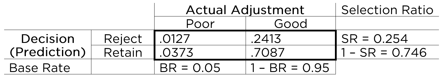
78% sounds pretty accurate. And it is much higher than 50%, so we are doing a pretty good job, right? Well, it is important to compare our accuracy to what accuracy we would expect to get by chance alone, if predictions were made by a random process rather than using a test’s scores. Our selection ratio was 25.4%. How accurate would we be if we randomly selected 25.4% of people to reject? To determine what accuracy we could get by chance alone given the selection ratio and the base rate, we can calculate the chance probability of true positives and the chance probability of true negatives. The probability of a given cell in the confusion matrix is a joint probability—the probability of two events occurring simultaneously. To calculate a joint probability, we multiply the probability of each event.
So, to get the chance expectancies of true positives, we would multiply the respective marginal probabilities, as in Equation 9.17:
\[ \begin{aligned} P(TP) &= P(\text{Poor adjustment}) \times P(\text{Reject})\\ &= BR \times SR \\ &= .05 \times .254 \\ &= .0127 \end{aligned} \tag{9.17}\]
To get the chance expectancies of true negatives, we would multiply the respective marginal probabilities, as in Equation 9.18:
\[ \begin{aligned} P(TN) &= P(\text{Good adjustment}) \times P(\text{Retain})\\ &= (1 - BR) \times (1 - SR) \\ &= .95 \times .746 \\ &= .7087 \end{aligned} \tag{9.18}\]
To get the percent accuracy by chance, we sum the chance expectancies for the correct predictions (TP and TN): \(.0127 + .7087 = .7214\). Thus, the percent accuracy you can get by chance alone is 72%. This is because most of our predictions are to retain people, and the base rate of poor adjustment is quite low (.05). Our measure with 78% accuracy provides only a 6% increment in correct predictions. Thus, you cannot judge how good your judgment or prediction is until you know how you would do by random chance.
The chance expectancies for each cell of the confusion matrix are in Figure 9.7.
9.1.2.4 Predicting from the Base Rate
Now, let us consider how well you would do if you were to predict from the base rate. Predicting from the base rate is also called “betting from the base rate”, and it involves setting the selection ratio by taking advantage of the base rate so that you go with the most likely outcome in every prediction. Because the base rate is quite low (.05), we could predict from the base rate by selecting no one to reject (i.e., setting the selection ratio at zero). Our percent accuracy by chance if we predict from the base rate would be calculated by multiplying the marginal probabilities, as we did above, but with a new selection ratio, as in Equation 9.19:
\[ \begin{aligned} P(TP) &= P(\text{Poor adjustment}) \times P(\text{Reject})\\ &= BR \times SR \\ &= .05 \times 0 \\ &= 0 \\ \\ P(TN) &= P(\text{Good adjustment}) \times P(\text{Retain})\\ &= (1 - BR) \times (1 - SR) \\ &= .95 \times 1 \\ &= .95 \end{aligned} \tag{9.19}\]
We sum the chance expectancies for the correct predictions (TP and TN): \(0 + .95 = .95\). Thus, our percent accuracy by predicting from the base rate is 95%. This is damning to our measure because it is a much higher accuracy than the accuracy of our measure. That is, we can be much more accurate than our measure simply by predicting from the base rate and selecting no one to reject.
Going with the most likely outcome in every prediction (predicting from the base rate) can be highly accurate (in terms of percent accuracy) as noted by Meehl & Rosen (1955), especially when the base rate is very low or very high. This should serve as an important reminder that we need to compare the accuracy of our measures to the accuracy by (1) random chance and (2) predicting from the base rate. There are several important implications of the impact of base rates on prediction accuracy. One implication is that using the same test in different settings with different base rates will markedly change the accuracy of the test. Oftentimes, using a test will actually decrease the predictive accuracy when the base rate deviates greatly from .50. But percent accuracy is not everything. Percent accuracy treats different kinds of errors as if they are equally important. However, the value we place on different kinds of errors may be different, as described next.
9.1.2.5 Different Kinds of Errors Have Different Costs
Some errors have a high cost, and some errors have a low cost. Among the four decision outcomes, there are two types of errors: false positives and false negatives. The extent to which false positives and false negatives are costly depends on the prediction problem. So, even though you can often be most accurate by going with the base rate, it may be advantageous to use a screening instrument despite lower overall accuracy because of the huge difference in costs of false positives versus false negatives in some cases.
Consider the example of a screening instrument for HIV. False positives would be cases where we said that someone is at high risk of HIV when they are not, whereas false negatives are cases where we said that someone is not at high risk when they actually are. The costs of false positives include a shortage of blood, some follow-up testing, and potentially some anxiety, but that is about it. The costs of false negatives may be people getting HIV. In this case, the costs of false negatives greatly outweigh the costs of false positives, so we use a screening instrument to try to identify the cases at high risk for HIV because of the important consequences of failing to do so, even though using the screening instrument will lower our overall accuracy level.
Another example is when the Central Intelligence Agency (CIA) used a screen for protective typists during wartime to try to detect spies. False positives would be cases where the CIA believes that a person is a spy when they are not, and the CIA does not hire them. False negatives would be cases where the CIA believes that a person is not a spy when they actually are, and the CIA hires them. In this case, a false positive would be fine, but a false negative would be really bad.
How you weigh the costs of different errors depends considerably on the domain and context. Possible costs of false positives to society include: unnecessary and costly treatment with side effects and sending an innocent person to jail (despite our presumption of innocence in the United States criminal justice system that a person is innocent until proven guilty). Possible costs of false negatives to society include: setting a guilty person free, failing to detect a bomb or tumor, and preventing someone from getting treatment who needs it.
The differential costs of different errors also depend on how much flexibility you have in the selection ratio in being able to set a stringent versus loose selection ratio. Consider if there is a high cost of getting rid of people during the selection process. For example, if you must hire 100 people and only 100 people apply for the position, you cannot lose people, so you need to hire even high-risk people. However, if you do not need to hire many people, then you can hire more conservatively.
Any time the selection ratio differs from the base rate, you will make errors. For example, if you reject 25% of applicants, and the base rate of poor adjustment is 5%, then you are making errors of over-rejecting (false positives). By contrast, if you reject 1% of applicants and the base rate of poor adjustment is 5%, then you are making errors of under-rejecting or over-accepting (false negatives).
A low base rate makes it harder to make predictions, and tends to lead to less accurate predictions. For instance, it is very challenging to predict low base rate behaviors, including suicide (Kessler et al., 2020). The difficulty in predicting events with a low base rate is apparent with the true score formula from classical test theory: \(X = T + e\). As described in Equation 4.10, reliability is the ratio of true score variance to observed score variance. As true score variance increases, reliability increases. If the base rate is .05, the maximum variance of the true scores is .05. The lower true score variance makes the measure less reliable and hard to make accurate predictions.
9.1.2.6 Sensitivity, Specificity, PPV, and NPV
As described earlier, percent accuracy is not the only important aspect of accuracy. Percent accuracy can be misleading because it is highly influenced by base rates. You can have a high percent accuracy by predicting from the base rate and saying that no one has the condition (if the base rate is low) or that everyone has the condition (if the base rate is high). Thus, it is also important to consider other aspects of accuracy, including sensitivity (SN), specificity (SP), positive predictive value (PPV), and negative predictive value (NPV). We want our predictions to be sensitive to be able to detect the characteristic but also to be specific so that we classify only people actually with the characteristic as having the characteristic.
Let us return to the confusion matrix in Figure 9.8. If we know the frequency of each of the four predicted-actual combinations of the confusion matrix (TP, TN, FP, FN), we can calculate sensitivity, specificity, PPV, and NPV.
: 2x2 Prediction Matrix. TP = true positives; TN = true negatives; FP = false positives; FN = false negatives.](images/2x2-Matrix_2e.png)
Sensitivity is the proportion of those with the characteristic (\(\text{TP} + \text{FN}\)) that we identified with our measure (\(\text{TP}\)): \(\frac{\text{TP}}{\text{TP} + \text{FN}} = \frac{86}{86 + 14} = .86\). Specificity is the proportion of those who do not have the characteristic (\(\text{TN} + \text{FP}\)) that we correctly classify as not having the characteristic (\(\text{TN}\)): \(\frac{\text{TN}}{\text{TN} + \text{FP}} = \frac{1,478}{1,478 + 422} = .78\). PPV is the proportion of those who we classify as having the characteristic (\(\text{TP} + \text{FP}\)) who actually have the characteristic (\(\text{TP}\)): \(\frac{\text{TP}}{\text{TP} + \text{FP}} = \frac{86}{86 + 422} = .17\). NPV is the proportion of those we classify as not having the characteristic (\(\text{TN} + \text{FN}\)) who actually do not have the characteristic (\(\text{TN}\)): \(\frac{\text{TN}}{\text{TN} + \text{FN}} = \frac{1,478}{1,478 + 14} = .99\).
Sensitivity, specificity, PPV, and NPV are proportions, and their values therefore range from 0 to 1, where higher values reflect greater accuracy. With sensitivity, specificity, PPV, and NPV, we have a good snapshot of how accurate the measure is at a given cutoff. In our case, our measure is good at finding whom to reject (high sensitivity), but it is rejecting too many people who do not need to be rejected (lower PPV due to many FPs). Most people whom we classify as having the characteristic do not actually have the characteristic. However, the fact that we are over-rejecting could be okay depending on our goals, for instance, if we do not care about over-dropping (i.e., the PPV being low).
9.1.2.6.1 Some Accuracy Estimates Depend on the Cutoff
Sensitivity, specificity, PPV, and NPV differ based on the cutoff (i.e., threshold) for classification. Consider the following example. Aliens visit Earth, and they develop a test to determine whether a berry is edible or inedible.
Code
library("tidyverse")
library("magrittr")
library("viridis")

sampleSize <- 1000

edibleScores <- rnorm(sampleSize, 50, 15)
inedibleScores <- rnorm(sampleSize, 100, 15)

edibleData <- data.frame(score = c(edibleScores, inedibleScores), type = c(rep("edible", sampleSize), rep("inedible", sampleSize)))

cutoff <- 75

hist_edible <- density(edibleScores, from = 0, to = 150) %$%
  data.frame(x = x, y = y) %>%
  mutate(area = x >= cutoff)

hist_edible$type[hist_edible$area == TRUE] <- "edible_FP"
hist_edible$type[hist_edible$area == FALSE] <- "edible_TN"

hist_inedible <- density(inedibleScores, from = 0, to = 150) %$%
  data.frame(x = x, y = y) %>%
  mutate(area = x < cutoff)

hist_inedible$type[hist_inedible$area == TRUE] <- "inedible_FN"
hist_inedible$type[hist_inedible$area == FALSE] <- "inedible_TP"

density_data <- bind_rows(hist_edible, hist_inedible)

density_data$type <- factor(density_data$type, levels = c("edible_TN","inedible_TP","edible_FP","inedible_FN"))
Figure 9.9 depicts the distributions of scores by berry type. Note how there are clearly two distinct distributions. However, the distributions overlap to some degree. Thus, any cutoff will have at least some inaccurate classifications. The extent of overlap of the distributions reflects the amount of measurement error of the measure with respect to the characteristic of interest.
Code
#No Cutoff
ggplot(data = edibleData, aes(x = score, ymin = 0, fill = type)) +
  geom_density(alpha = .5) +
  scale_fill_manual(name = "Berry Type", values = c(viridis(2)[2], viridis(2)[1])) +
  scale_y_continuous(name = "Frequency") +
  theme_bw() +
  theme(axis.text.y = element_blank(),
        axis.ticks.y = element_blank())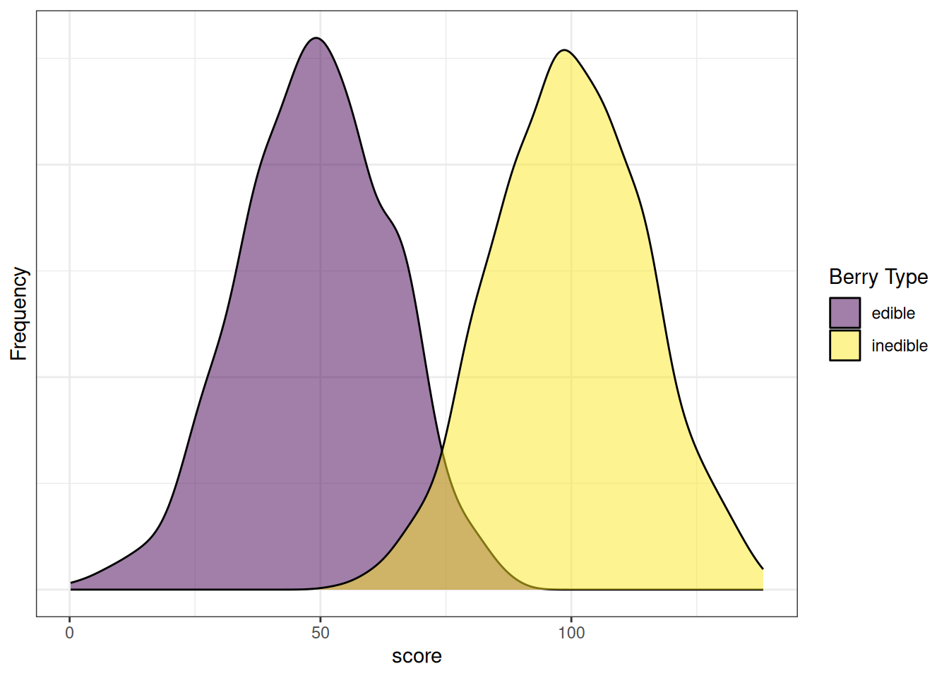
Figure 9.10 depicts the distributions of scores by berry type with a cutoff. The red line indicates the cutoff—the level above which berries are classified by the test as inedible. There are errors on each side of the cutoff. Below the cutoff, there are some false negatives (blue): inedible berries that are inaccurately classified as edible. Above the cutoff, there are some false positives (green): edible berries that are inaccurately classified as inedible. Costs of false negatives could include sickness or death from eating the inedible berries. Costs of false positives could include taking longer to find food, finding insufficient food, and starvation.
Code
#Standard Cutoff
ggplot(data = density_data, aes(x = x, ymin = 0, ymax = y, fill = type)) +
  geom_ribbon(alpha = 1) +
  scale_fill_manual(name = "Berry Type",
                    values = c(viridis(4)[4], viridis(4)[1], viridis(4)[3], viridis(4)[2]),
                    breaks = c("edible_TN","inedible_TP","edible_FP","inedible_FN"),
                    labels = c("Edible: TN","Inedible: TP","Edible: FP","Inedible: FN")) +
  geom_line(aes(y = y)) +
  geom_vline(xintercept = cutoff, color = "red", linewidth = 2) +
  scale_x_continuous(name = "score") +
  scale_y_continuous(name = "Frequency") +
  theme_bw() +
  theme(axis.text.y = element_blank(),
        axis.ticks.y = element_blank())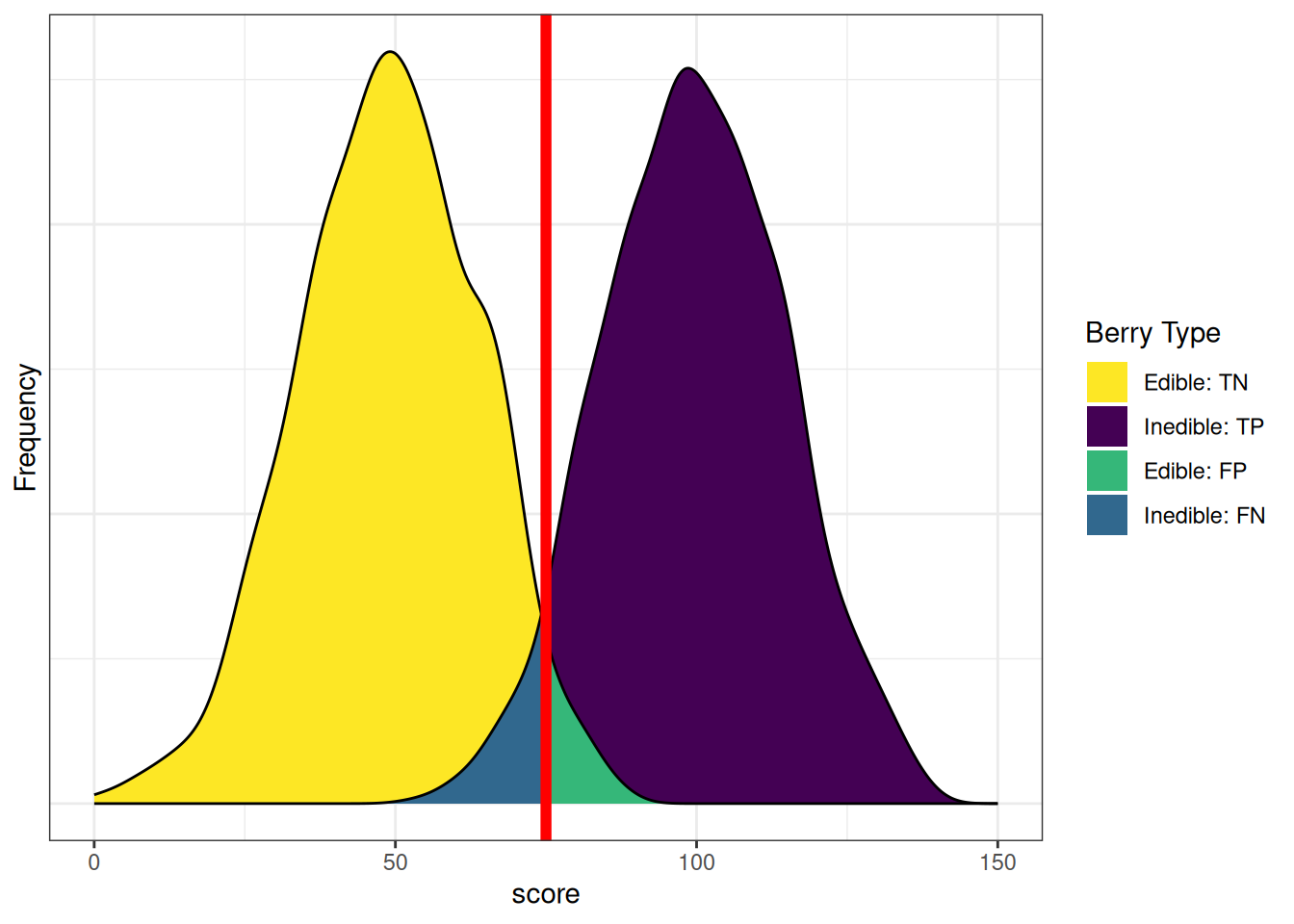
Based on our assessment goals, we might use a different selection ratio by changing the cutoff. Figure 9.11 depicts the distributions of scores by berry type when we raise the cutoff. There are now more false negatives (blue) and fewer false positives (green). If we raise the cutoff (to be more conservative), the number of false negatives increases and the number of false positives decreases. Consequently, as the cutoff increases, sensitivity and NPV decrease (because we have more false negatives), whereas specificity and PPV increase (because we have fewer false positives). A higher cutoff could be optimal if the costs of false positives are considered greater than the costs of false negatives. For instance, if the aliens cannot risk eating the inedible berries because the berries are fatal, and there are sufficient edible berries that can be found to feed the alien colony.
Code
#Raise the cutoff
cutoff <- 85

hist_edible <- density(edibleScores, from = 0, to = 150) %$%
  data.frame(x = x, y = y) %>%
  mutate(area = x >= cutoff)

hist_edible$type[hist_edible$area == TRUE] <- "edible_FP"
hist_edible$type[hist_edible$area == FALSE] <- "edible_TN"

hist_inedible <- density(inedibleScores, from = 0, to = 150) %$%
  data.frame(x = x, y = y) %>%
  mutate(area = x < cutoff)

hist_inedible$type[hist_inedible$area == TRUE] <- "inedible_FN"
hist_inedible$type[hist_inedible$area == FALSE] <- "inedible_TP"

density_data <- bind_rows(hist_edible, hist_inedible)

density_data$type <- factor(density_data$type, levels = c("edible_TN","inedible_TP","edible_FP","inedible_FN"))

ggplot(data = density_data, aes(x = x, ymin = 0, ymax = y, fill = type)) +
  geom_ribbon(alpha = 1) +
  scale_fill_manual(name = "Berry Type",
                    values = c(viridis(4)[4], viridis(4)[1], viridis(4)[3], viridis(4)[2]),
                    breaks = c("edible_TN","inedible_TP","edible_FP","inedible_FN"),
                    labels = c("Edible: TN","Inedible: TP","Edible: FP","Inedible: FN")) +
  geom_line(aes(y = y)) +
  geom_vline(xintercept = cutoff, color = "red", linewidth = 2) +
  scale_x_continuous(name = "score") +
  scale_y_continuous(name = "Frequency") +
  theme_bw() +
  theme(axis.text.y = element_blank(),
        axis.ticks.y = element_blank())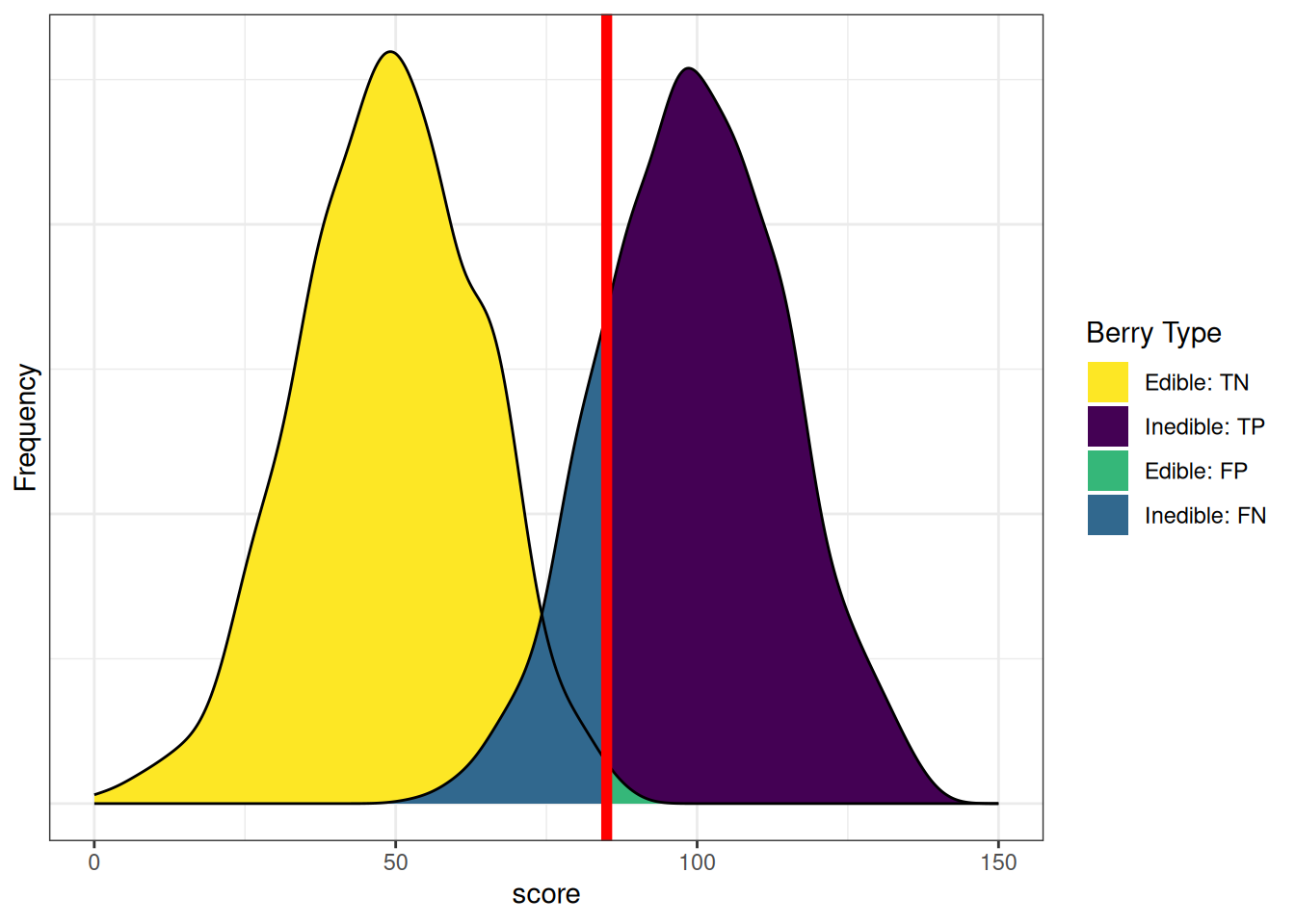
Figure 9.12 depicts the distributions of scores by berry type when we lower the cutoff. There are now fewer false negatives (blue) and more false positives (green). If we lower the cutoff (to be more liberal), the number of false negatives decreases and the number of false positives increases. Consequently, as the cutoff decreases, sensitivity and NPV increase (because we have fewer false negatives), whereas specificity and PPV decrease (because we have more false positives). A lower cutoff could be optimal if the costs of false negatives are considered greater than the costs of false positives. For instance, if the aliens cannot risk missing edible berries because they are in short supply relative to the size of the alien colony, and eating the inedible berries would, at worst, lead to minor, temporary discomfort.
Code
#Lower the cutoff
cutoff <- 65

hist_edible <- density(edibleScores, from = 0, to = 150) %$%
  data.frame(x = x, y = y) %>%
  mutate(area = x >= cutoff)

hist_edible$type[hist_edible$area == TRUE] <- "edible_FP"
hist_edible$type[hist_edible$area == FALSE] <- "edible_TN"

hist_inedible <- density(inedibleScores, from = 0, to = 150) %$%
  data.frame(x = x, y = y) %>%
  mutate(area = x < cutoff)

hist_inedible$type[hist_inedible$area == TRUE] <- "inedible_FN"
hist_inedible$type[hist_inedible$area == FALSE] <- "inedible_TP"

density_data <- bind_rows(hist_edible, hist_inedible)

density_data$type <- factor(density_data$type, levels = c("edible_TN","inedible_TP","edible_FP","inedible_FN"))

ggplot(data = density_data, aes(x = x, ymin = 0, ymax = y, fill = type)) +
  geom_ribbon(alpha = 1) +
  scale_fill_manual(name = "Berry Type",
                    values = c(viridis(4)[4], viridis(4)[1], viridis(4)[3], viridis(4)[2]),
                    breaks = c("edible_TN","inedible_TP","edible_FP","inedible_FN"),
                    labels = c("Edible: TN","Inedible: TP","Edible: FP","Inedible: FN")) +
  geom_line(aes(y = y)) +
  geom_vline(xintercept = cutoff, color = "red", linewidth = 2) +
  scale_x_continuous(name = "score") +
  scale_y_continuous(name = "Frequency") +
  theme_bw() +
  theme(axis.text.y = element_blank(),
        axis.ticks.y = element_blank())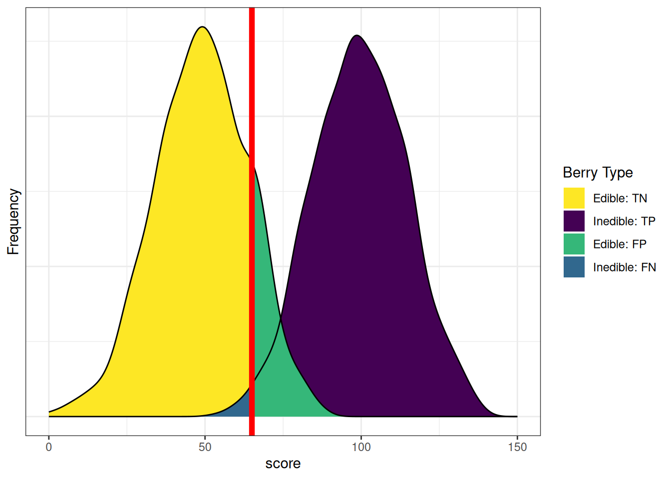
In sum, sensitivity and specificity differ based on the cutoff for classification. if we raise the cutoff, sensitivity and PPV increase (due to fewer false positives), whereas and sensitivity and NPV decrease (due to more false negatives). If we lower the cutoff, sensitivity and NPV increase (due to fewer false negatives), whereas specificity and PPV decrease (due to more false positives). Thus, the optimal cutoff depends on how costly each type of error is: false negatives and false positives. If false negatives are more costly than false positives, we would set a low cutoff. If false positives are more costly than false negatives, we would set a high cutoff.
9.1.2.7 Signal Detection Theory
Signal detection theory (SDT) is a probability-based theory for the detection of a given stimulus (signal) from a stimulus set that includes non-target stimuli (noise). SDT arose through the development of radar (RAdio Detection And Ranging) and sonar (SOund Navigation And Ranging) in World War II based on research on sensory-perception research. The military wanted to determine which objects on radar/sonar were enemy aircraft/submarines, and which were noise (e.g., different object in the environment or even just the weather itself). SDT allowed determining how many errors operators made (how accurate they were) and decomposing errors into different kinds of errors. SDT distinguishes between sensitivity and bias. In SDT, sensitivity (or discriminability) is how well an assessment distinguishes between a target stimulus and non-target stimuli (i.e., how well the assessment detects the target stimulus amid non-target stimuli). Bias is the extent to which the probability of a selection decision from the assessment is higher or lower than the true rate of the target stimulus.
Some radar/sonar operators were not as sensitive to the differences between signal and noise, due to factors such as age, ability to distinguish gradations of a signal, etc. People who showed low sensitivity (i.e., who were not as successful at distinguishing between signal and noise) were screened out because the military perceived sensitivity as a skill that was not easily taught. By contrast, other operators could distinguish signal from noise, but their threshold was too low or high—they could take in information, but their decisions tended to be wrong due to systematic bias or poor calibration. That is, they systematically over-rejected or under-rejected stimuli. Over-rejecting leads to many false negatives (i.e., saying that a stimulus is safe when it is not). Under-rejecting leads to many false positives (i.e., saying that a stimulus is harmful when it is not). A person who showed good sensitivity but systematic bias was considered more teach-able than a person who showed low sensitivity. Thus, radar and sonar operators were selected based on their sensitivity to distinguish signal from noise, and then were trained to improve the calibration so they reduce their systematic bias and do not systematically over- or under-reject.
Although SDT was originally developed for use in World War II, it now plays an important role in many areas of science and medicine. A medical application of SDT is tumor detection in radiology. SDT also plays an important role in psychology, especially cognitive psychology. For instance, research on social perception of sexual interest has shown that men tend to show lack of sensitivity to differences in women’s affect—i.e., they have relative difficulties discriminating between friendliness and sexual interest (Farris et al., 2008). Men also tend to show systematic bias (poor calibration) such that they tend to over-estimate women’s sexual interest in them—i.e., men tend to have too low of a threshold for determining that a women is showing sexual interest in them (Farris et al., 2006).
SDT metrics of sensitivity include \(d'\) (“\(d\)-prime”), \(A\) (or \(A'\)), and the area under the receiver operating characteristic (ROC) curve. SDT metrics of bias include \(\beta\) (beta), \(c\), and \(b\).
9.1.2.7.1 Receiver Operating Characteristic (ROC) Curve
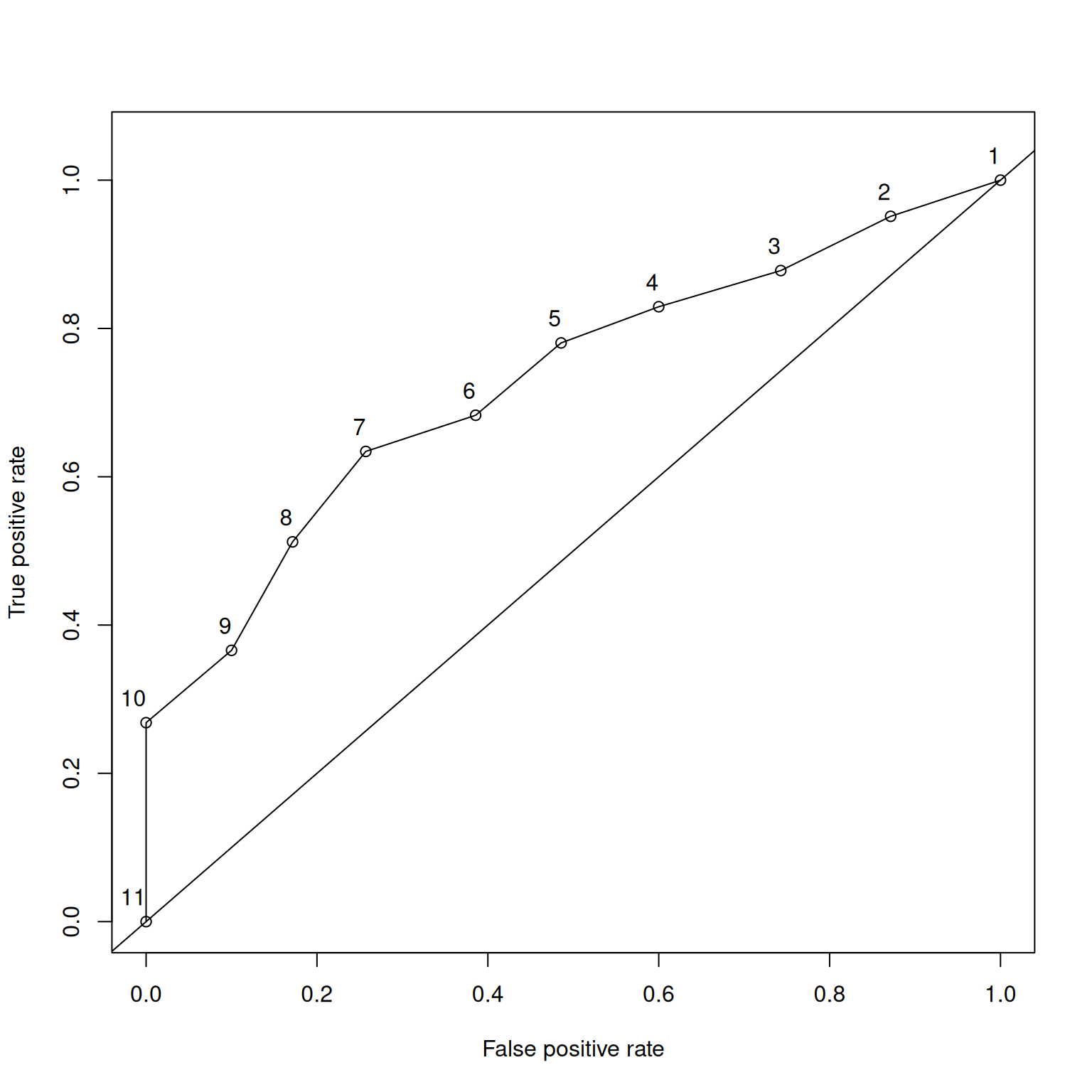
The x-axis of the ROC curve is the false alarm rate or false positive rate (\(1 -\) specificity). The y-axis is the hit rate or true positive rate (sensitivity). We can trace the ROC curve as the combination between sensitivity and specificity at every possible cutoff. At a cutoff of zero (top right of ROC curve), we calculate sensitivity (1.0) and specificity (0) and plot it. At a cutoff of zero, the assessment tells us to make an action for every stimulus (i.e., it is the most liberal). We then gradually increase the cutoff, and plot sensitivity and specificity at each cutoff. As the cutoff increases, sensitivity decreases and specificity increases. We end at the highest possible cutoff, where the sensitivity is 0 and the specificity is 1.0 (i.e., we never make an action; i.e., it is the most conservative). Each point on the ROC curve corresponds to a pair of hit and false alarm rates (sensitivity and specificity) resulting from a specific cutoff value. Then, we can draw lines or a curve to connect the points.
Figure 9.13 depicts an empirical ROC plot where lines are drawn to connect the hit and false alarm rates.
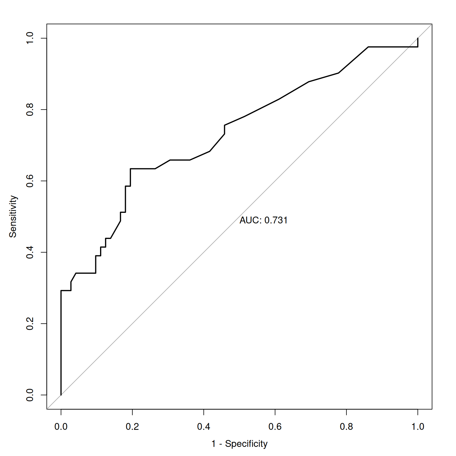
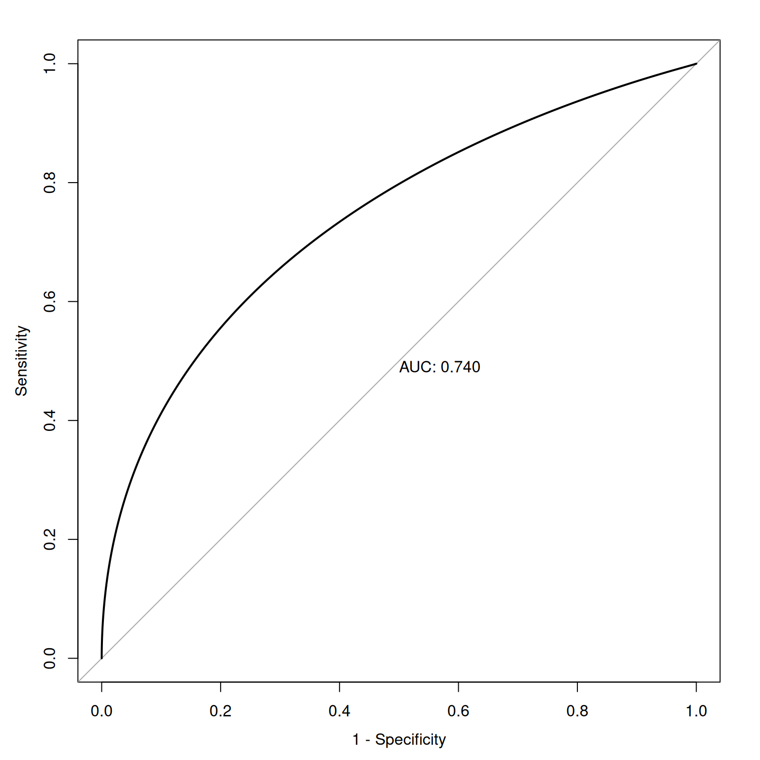
Figure 9.14 depicts an ROC curve where a smoothed and fitted curve is drawn to connect the hit and false alarm rates.
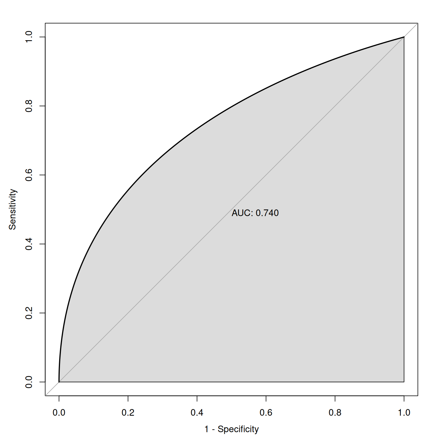
9.1.2.7.1.1 Area Under the ROC Curve
ROC methods can be used to compare and compute the discriminative power of measurement devices free from the influence of selection ratios, base rates, and costs and benefits. An ROC analysis yields a quantitative index of how well an index predicts a signal of interest or can discriminate between different signals. ROC analysis can help tell us how often our assessment would be correct. If we randomly pick two observations, and we were right once and wrong once, we were 50% accurate. But this would be a useless measure because it reflects chance responding.
The geometrical area under the ROC curve reflects the discriminative accuracy of the measure. The index is called the area under the curve (AUC) of an ROC curve. AUC quantifies the discriminative power of an assessment. AUC is the probability that a randomly selected target and a randomly selected non-target is ranked correctly by the assessment method. AUC values range from 0.0 to 1.0, where chance accuracy is 0.5 as indicated by diagonal line in the ROC curve. That is, a measure can be useful to the extent that its ROC curve is above the diagonal line (i.e., its discriminative accuracy is above chance).
Code
Code
#From here: https://stats.stackexchange.com/questions/422926/generate-synthetic-data-given-auc/424213; archived at https://perma.cc/F6F9-VG2K
simulateDataFromAUC <- function(auc, n){
  t <- sqrt(log(1/(1-auc)**2))
  z <- t-((2.515517 + 0.802853*t + 0.0103328*t**2) / (1 + 1.432788*t + 0.189269*t**2 + 0.001308*t**3))
  d <- z*sqrt(2)

  x <- c(rnorm(n/2, mean = 0), rnorm(n/2, mean = d))
  y <- c(rep(0, n/2), rep(1, n/2))

  data <- data.frame(x = x, y = y)

return(data)
}

set.seed(52242)

auc60 <- simulateDataFromAUC(.60, 50000)
auc70 <- simulateDataFromAUC(.70, 50000)
auc80 <- simulateDataFromAUC(.80, 50000)
auc90 <- simulateDataFromAUC(.90, 50000)
auc95 <- simulateDataFromAUC(.95, 50000)
auc99 <- simulateDataFromAUC(.99, 50000)

plot(roc(y ~ x, auc60, smooth = TRUE), legacy.axes = TRUE, print.auc = TRUE, print.auc.x = .52, print.auc.y = .61, print.auc.pattern = "%.2f")
plot(roc(y ~ x, auc70, smooth = TRUE), legacy.axes = TRUE, print.auc = TRUE, print.auc.x = .6, print.auc.y = .67, print.auc.pattern = "%.2f", add = TRUE)
plot(roc(y ~ x, auc80, smooth = TRUE), legacy.axes = TRUE, print.auc = TRUE, print.auc.x = .695, print.auc.y = .735, print.auc.pattern = "%.2f", add = TRUE)
plot(roc(y ~ x, auc90, smooth = TRUE), legacy.axes = TRUE, print.auc = TRUE, print.auc.x = .805, print.auc.y = .815, print.auc.pattern = "%.2f", add = TRUE)
plot(roc(y ~ x, auc95, smooth = TRUE), legacy.axes = TRUE, print.auc = TRUE, print.auc.x = .875, print.auc.y = .865, print.auc.pattern = "%.2f", add = TRUE)
plot(roc(y ~ x, auc99, smooth = TRUE), legacy.axes = TRUE, print.auc = TRUE, print.auc.x = .94, print.auc.y = .94, print.auc.pattern = "%.2f", add = TRUE)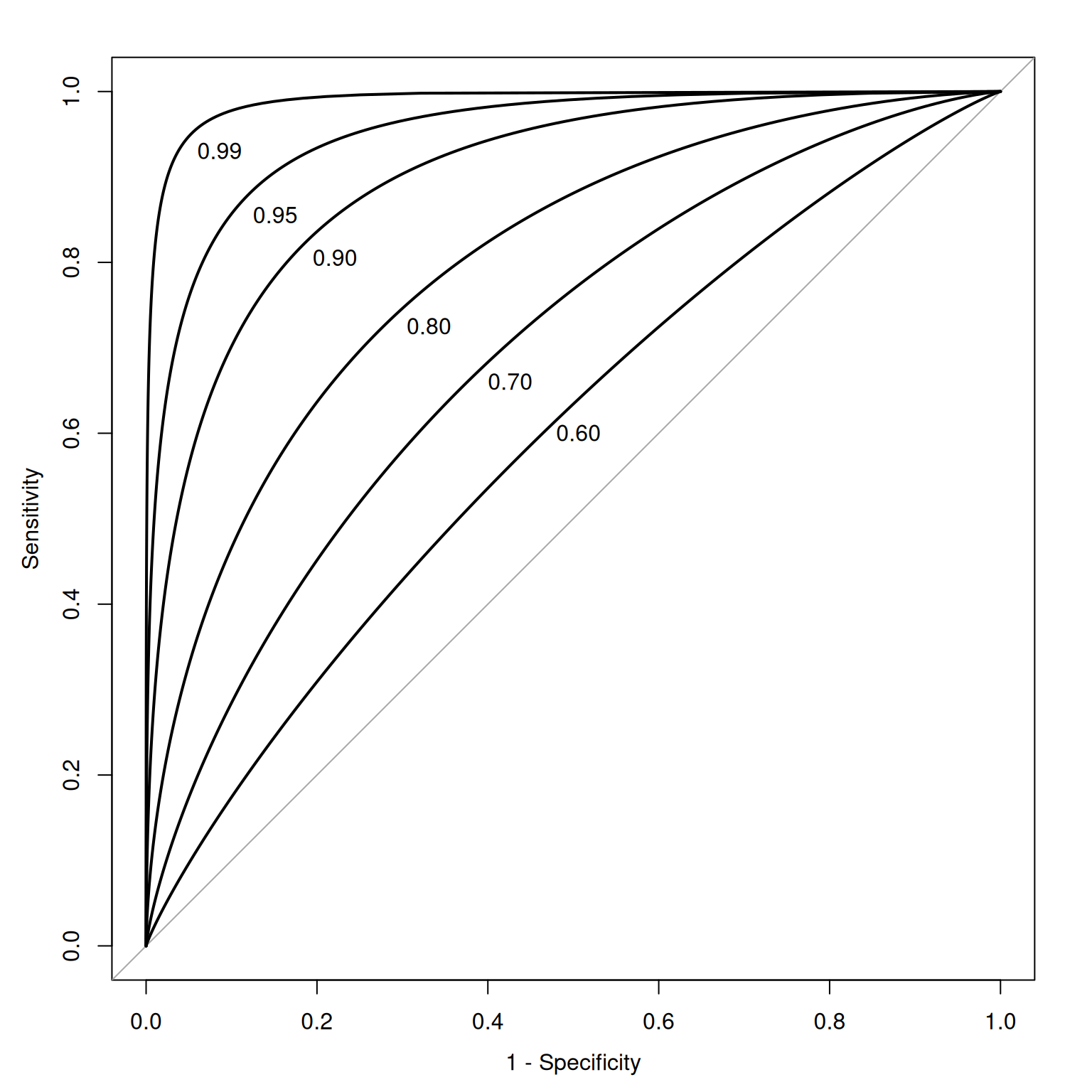
As an example, given an AUC of .75, this says that the overall score of an individual who has the characteristic in question will be higher 75% of the time than the overall score of an individual who does not have the characteristic. In lay terms, AUC provides the probability that we will classify correctly based on our instrument if we were to randomly pick one good and one bad outcome. AUC is a stronger index of accuracy than percent accuracy, because you can have high percent accuracy just by going with the base rate. AUC tells us how much better than chance a measure is at discriminating outcomes. AUC is useful as a measure of general discriminative accuracy, and it tells us how accurate a measure is at all possible cutoffs. Knowing the accuracy of a measure at all possible cutoffs can be helpful for selecting the optimal cutoff, given the goals of the assessment. In reality, however, we may not be interested in all cutoffs because not all errors are equal in their costs.
If we lower the base rate, we would need a larger sample to get enough people to classify into each group. SDT/ROC methods are traditionally about dichotomous decisions (yes/no), not graded judgments. SDT/ROC methods can get messy with ordinal data that are more graded because you would have an AUC curve for each ordinal grouping.
9.2 Getting Started
9.2.1 Load Libraries
Code
library("petersenlab") #to install: install.packages("remotes"); remotes::install_github("DevPsyLab/petersenlab")
library("pROC")
library("ROCR")
library("rms")
library("ResourceSelection")
library("PredictABEL")
library("uroc") #to install: install.packages("remotes"); remotes::install_github("evwalz/uroc")
library("rms")
library("gridExtra")
library("grid")
library("ggpubr")
library("msir")
library("car")
library("viridis")
library("ggrepel")
library("caret")
library("MOTE")
library("tidyverse")
library("here")
library("tinytex")
library("rmarkdown")
library("knitr")
9.2.2 Prepare Data
9.2.2.1 Load Data
aSAH is a data set from the pROC package (Robin et al., 2021) that contains test scores (s100b) and clinical outcomes (outcome) for patients.
9.2.2.2 Simulate Data
For reproducibility, I set the seed below. Using the same seed will yield the same answer every time. There is nothing special about this particular seed.
Code
set.seed(52242)

mydataSDT$testScore <- mydataSDT$s100b
mydataSDT <- mydataSDT %>%
  mutate(testScoreSimple = ntile(testScore, 10))

mydataSDT$predictedProbability <-
  (mydataSDT$s100b - min(mydataSDT$s100b, na.rm = TRUE)) /
  (max(mydataSDT$s100b, na.rm = TRUE) - min(mydataSDT$s100b, na.rm = TRUE))
mydataSDT$continuousOutcome <- mydataSDT$testScore +
  rnorm(nrow(mydataSDT), mean = 0.20, sd = 0.20)
mydataSDT$disorder <- NA
mydataSDT$disorder[mydataSDT$outcome == "Good"] <- 0
mydataSDT$disorder[mydataSDT$outcome == "Poor"] <- 1
9.2.2.3 Add Missing Data
Adding missing data to dataframes helps make examples more realistic to real-life data and helps you get in the habit of programming to account for missing data.
9.3 Receiver Operating Characteristic (ROC) Curve
The receiver operating characteristic (ROC) curve shows the combination of hit rate (sensitivity) and false alarm rate (\(1 - \text{specificity}\)) at every possible cutoff. It depicts that, as the cutoff increases (i.e., becomes more conservative), sensitivity decreases and specificity increases. It also depicts that, as the cutoff decreases (i.e., becomes more liberal), sensitivity increases and specificity decreases.
Receiver operating characteristic (ROC) curves were generated using the pROC package (Robin et al., 2021). The examples depict ROC curves that demonstrate that the measure is moderately accurate—the measure is more accurate than chance but there remains considerable room for improvement in predictive accuracy.
9.3.1 Empirical ROC Curve
The syntax used to generate an empirical ROC plot is below, and the plot is in Figure 9.13.

An empirical ROC plot with cutoffs overlaid is in Figure 9.18.
Code
9.3.2 Smooth ROC Curve

9.3.3 Youden’s J Statistic
The threshold at the Youden’s J statistic is the threshold where the test has the maximum combination (i.e., sum) of sensitivity and specificity: \(\text{max}(\text{sensitivity} + \text{specificity} - 1)\)
Code
For this test, the Youden’s J Statistic is at a threshold of \(0.205\), where sensitivity is \(0.65\) and specificity is \(0.8\).
9.3.4 The point closest to the top-left part of the ROC curve with perfect sensitivity and specificity
The point closest to the top-left part of the ROC plot with perfect sensitivity and specificity: \(\text{min}[(1 - \text{sensitivity})^2 + (1 - \text{specificity})^2]\)
Code
For this test, the combination of sensitivity and specificity is closest to the top left of the ROC plot at a threshold of \(0.205\), where sensitivity is \(0.65\) and specificity is \(0.8\).
9.4 Prediction Accuracy Across Cutoffs
There are two primary dimensions of accuracy: (1) discrimination (e.g., sensitivity, specificity, area under the ROC curve) and (2) calibration. Some general indexes of accuracy combine discrimination and calibration, as described in Section 9.4.1. This section (Section 9.4) describes indexes of accuracy that span all possible cutoffs. That is, each index of accuracy described in this section provides a single numerical index of accuracy that aggregates the accuracy across all possible cutoffs. Aspects of accuracy at a particular cutoff are described in Section 9.5.
The petersenlab package (Petersen, 2025) contains the accuracyOverall() function that estimates the prediction accuracy across cutoffs.
Code
                               [,1]
ME                            -0.11
MAE                            0.34
MdAE                           0.17
MSE                            0.21
RMSE                           0.46
MPE                            -Inf
MAPE                            Inf
sMAPE                         82.46
MASE                           0.74
RMSLE                          0.30
rsquared                       0.10
rsquaredAsPredictor            0.18
rsquaredAdjAsPredictor         0.17
rsquaredPredictiveAsPredictor  0.12
Code
                               [,1]
ME                            -0.11
MAE                            0.34
MdAE                           0.17
MSE                            0.21
RMSE                           0.46
MPE                           59.62
MAPE                          64.97
sMAPE                         82.46
MASE                           0.74
RMSLE                          0.30
rsquared                       0.10
rsquaredAsPredictor            0.18
rsquaredAdjAsPredictor         0.17
rsquaredPredictiveAsPredictor  0.12
9.4.1 General Prediction Accuracy
There are many metrics of general prediction accuracy. When thinking about which metric(s) may be best for a given problem, it is important to consider the purpose of the assessment. The estimates of general prediction accuracy are separated below into scale-dependent and scale-independent accuracy estimates.
9.4.1.1 Scale-Dependent Accuracy Estimates
The estimates of prediction accuracy described in this section are scale-dependent. These accuracy estimates depend on the unit of measurement and therefore cannot be compared across measures with different scales or across data sets.
9.4.1.1.1 Mean Error
Here, “error” (\(e\)) is the difference between the predicted and observed value for a given individual (\(i\)). Mean error (ME; also known as bias, see Section 4.5.1.3.2) is the mean difference between the predicted and observed values across individuals (\(i\)), that is, the mean of the errors across individuals (\(e_i\)). Values closer to zero reflect greater accuracy. If mean error is above zero, it indicates that predicted values are, on average, greater than observed values (i.e., over-estimating errors). If mean error is below zero, it indicates that predicted values are, on average, less than observed values (i.e., under-estimating errors). If both over-estimating and under-estimating errors are present, however, they can cancel each other out. As a result, even with a mean error of zero, there can still be considerable error present. Thus, although mean error can be helpful for examining whether predictions systematically under- or over-estimate the actual scores, other forms of accuracy are necessary to examine the extent of error. The formula for mean error is in Equation 9.20:
\[ \begin{aligned} \text{mean error} &= \frac{\sum\limits_{i = 1}^n(\text{predicted}_i - \text{observed}_i)}{n} \\ &= \text{mean}(e_i) \end{aligned} \tag{9.20}\]
In this case, the mean error is negative, so the predictions systematically under-estimate the actual scores.
9.4.1.1.2 Mean Absolute Error (MAE)
Mean absolute error (MAE) is the mean of the absolute value of differences between the predicted and observed values across individuals, that is, the mean of the absolute value of errors. Smaller MAE values (closer to zero) reflect greater accuracy. MAE is preferred over root mean squared error (RMSE) when you want to give equal weight to all errors and when the outliers have considerable impact. The formula for MAE is in Equation 9.21:
\[ \begin{aligned} \text{mean absolute error (MAE)} &= \frac{\sum\limits_{i = 1}^n|\text{predicted}_i - \text{observed}_i|}{n} \\ &= \text{mean}(|e_i|) \end{aligned} \tag{9.21}\]
9.4.1.1.3 Mean Squared Error (MSE)
Mean squared error (MSE) is the mean of the square of the differences between the predicted and observed values across individuals, that is, the mean of the squared value of errors. Smaller MSE values (closer to zero) reflect greater accuracy. MSE penalizes larger errors more heavily than smaller errors (unlike MAE). However, MSE is sensitive to outliers and can be impacted if the errors are skewed. The formula for MSE is in Equation 9.22:
\[ \begin{aligned} \text{mean squared error (MSE)} &= \frac{\sum\limits_{i = 1}^n(\text{predicted}_i - \text{observed}_i)^2}{n} \\ &= \text{mean}(e_i^2) \end{aligned} \tag{9.22}\]
9.4.1.1.4 Root Mean Squared Error (RMSE)
Root mean squared error (RMSE) is the square root of the mean of the square of the differences between the predicted and observed values across individuals, that is, the root mean squared value of errors. Smaller RMSE values (closer to zero) reflect greater accuracy. RMSE penalizes larger errors more heavily than smaller errors (unlike MAE). However, RMSE is sensitive to outliers and can be impacted if the errors are skewed. The formula for RMSE is in Equation 9.23:
\[ \begin{aligned} \text{root mean squared error (RMSE)} &= \sqrt{\frac{\sum\limits_{i = 1}^n(\text{predicted}_i - \text{observed}_i)^2}{n}} \\ &= \sqrt{\text{mean}(e_i^2)} \end{aligned} \tag{9.23}\]
9.4.1.2 Scale-Independent Accuracy Estimates
The estimates of prediction accuracy described in this section are intended to be scale-independent (unit-free) so the accuracy estimates can be compared across measures with different scales or across data sets (Hyndman & Athanasopoulos, 2018).
9.4.1.2.1 Mean Percentage Error (MPE)
Mean percentage error (MPE) values closer to zero reflect greater accuracy. The formula for percentage error is in Equation 9.24:
\[ \begin{aligned} \text{percentage error }(p_i) = \frac{100\% \times (\text{observed}_i - \text{predicted}_i)}{\text{observed}_i} \end{aligned} \tag{9.24}\]
We then take the mean of the percentage errors to get MPE. The formula for MPE is in Equation 9.25:
\[ \begin{aligned} \text{mean percentage error (MPE)} &= \frac{100\%}{n} \sum\limits_{i = 1}^n \frac{\text{observed}_i - \text{predicted}_i}{\text{observed}_i} \\ &= \text{mean(percentage error)} \\ &= \text{mean}(p_i) \end{aligned} \tag{9.25}\]
Note: MPE is undefined when one or more of the observed values equals zero, due to division by zero. I provide the option in the function to drop undefined values so you can still generate an estimate of accuracy despite undefined values, but use this option at your own risk.
9.4.1.2.2 Mean Absolute Percentage Error (MAPE)
Smaller mean absolute percentage error (MAPE) values (closer to zero) reflect greater accuracy. The formula for MAPE is in Equation 9.26: MAPE is asymmetric because it overweights underestimates and underweights overestimates. MAPE can be preferable to symmetric mean absolute percentage error (sMAPE) if there are no observed values of zero and if you want to emphasize the importance of underestimates (relative to overestimates).
\[ \begin{aligned} \text{mean absolute percentage error (MAPE)} &= \frac{100\%}{n} \sum\limits_{i = 1}^n \Bigg|\frac{\text{observed}_i - \text{predicted}_i}{\text{observed}_i}\Bigg| \\ &= \text{mean(|percentage error|)} \\ &= \text{mean}(|p_i|) \end{aligned} \tag{9.26}\]
Note: MAPE is undefined when one or more of the observed values equals zero, due to division by zero. I provide the option in the function to drop undefined values so you can still generate an estimate of accuracy despite undefined values, but use this option at your own risk.
9.4.1.2.3 Symmetric Mean Absolute Percentage Error (sMAPE)
Unlike MAPE, symmetric mean absolute percentage error (sMAPE) is symmetric because it equally weights underestimates and overestimates. Smaller sMAPE values (closer to zero) reflect greater accuracy. The formula for sMAPE is in Equation 9.27:
\[ \small \begin{aligned} \text{symmetric mean absolute percentage error (sMAPE)} = \frac{100\%}{n} \sum\limits_{i = 1}^n \frac{|\text{predicted}_i - \text{observed}_i|}{|\text{predicted}_i| + |\text{observed}_i|} \end{aligned} \tag{9.27}\]
Note: sMAPE is undefined when one or more of the individuals has a prediction–observed combination such that the sum of the absolute value of the predicted value and the absolute value of the observed value equals zero (\(|\text{predicted}_i| + |\text{observed}_i|\)), due to division by zero. I provide the option in the function to drop undefined values so you can still generate an estimate of accuracy despite undefined values, but use this option at your own risk.
Code
symmetricMeanAbsolutePercentageError = function(predicted, actual, dropUndefined = FALSE){
  relativeError <- abs(predicted - actual)/(abs(predicted) + abs(actual))

  if(dropUndefined == TRUE){
    relativeError[!is.finite(relativeError)] <- NA
  }

  value <- 100 * mean(abs(relativeError), na.rm = TRUE)
  return(value)
}9.4.1.2.4 Mean Absolute Scaled Error (MASE)
Mean absolute scaled error (MASE) is described by (Hyndman & Athanasopoulos, 2018). Values closer to zero reflect greater accuracy.
The adapted formula for MASE with non-time series data is described here (https://stats.stackexchange.com/a/108963/20338) (archived at https://perma.cc/G469-8NAJ). Scaled errors are calculated using Equation 9.28:
\[ \begin{aligned} \text{scaled error}(q_i) &= \frac{\text{observed}_i - \text{predicted}_i}{\text{scaling factor}} \\ &= \frac{\text{observed}_i - \text{predicted}_i}{\frac{1}{n} \sum\limits_{i = 1}^n |\text{observed}_i - \overline{\text{observed}}|} \end{aligned} \tag{9.28}\]
Then, we calculate the mean of the absolute value of the scaled errors to get MASE, as in Equation 9.29:
\[ \begin{aligned} \text{mean absolute scaled error (MASE)} &= \frac{1}{n} \sum\limits_{i = 1}^n |q_i| \\ &= \text{mean(|scaled error|)} \\ &= \text{mean}(|q_i|) \end{aligned} \tag{9.29}\]
Note: MASE is undefined when the scaling factor is zero, due to division by zero. With non-time series data, the scaling factor is the average of the absolute value of individuals’ observed scores minus the average observed score (\(\frac{1}{n} \sum\limits_{i = 1}^n |\text{observed}_i - \overline{\text{observed}}|\)).
Code
meanAbsoluteScaledError <- function(predicted, actual){
  mydata <- data.frame(na.omit(cbind(predicted, actual)))

  errors <- mydata$actual - mydata$predicted
  scalingFactor <- mean(abs(mydata$actual - mean(mydata$actual)))
  scaledErrors <- errors/scalingFactor

  value <- mean(abs(scaledErrors))
  return(value)
}9.4.1.2.5 Root Mean Squared Log Error (RMSLE)
The squared log of the accuracy ratio is described by Tofallis (2015). The accuracy ratio is in Equation 9.30:
\[ \begin{aligned} \text{accuracy ratio} &= \frac{\text{predicted}_i}{\text{observed}_i} \end{aligned} \tag{9.30}\]
However, the accuracy ratio is undefined with observed or predicted values of zero, so it is common to modify it by adding 1 to the predictor and denominator, as in Equation 9.31:
\[ \begin{aligned} \text{accuracy ratio} &= \frac{\text{predicted}_i + 1}{\text{observed}_i + 1} \end{aligned} \tag{9.31}\]
Squaring the log values keeps the values positive, such that smaller values (values closer to zero) reflect greater accuracy. Then we take the mean of the squared log values, which keeps the values positive, and calculate the square root of the mean squared log values to put them back on the (pre-squared) log metric. This is known as the root mean squared log error (RMSLE). Division inside the log is equal to subtraction outside the log. So, the formula can be reformulated with the subtraction of two logs, as in Equation 9.32:
\[ \begin{aligned} \text{root mean squared log error (RMSLE)} &= \sqrt{\sum\limits_{i = 1}^n log\bigg(\frac{\text{predicted}_i + 1}{\text{observed}_i + 1}\bigg)^2} \\ &= \sqrt{\text{mean}\Bigg[log\bigg(\frac{\text{predicted}_i + 1}{\text{observed}_i + 1}\bigg)^2\Bigg]} \\ &= \sqrt{\text{mean}\big[log(\text{accuracy ratio})^2\big]} = \sqrt{\text{mean}\Big\{\big[log(\text{predicted}_i + 1) - log(\text{actual}_i + 1)\big]^2\Big\}} \end{aligned} \tag{9.32}\]
RMSLE can be preferable when the scores have a wide range of values and are skewed. RMSLE can help to reduce the impact of outliers. RMSLE gives more weight to smaller errors in the prediction of small observed values, while also penalizing larger errors in the prediction of larger observed values. It overweights underestimates and underweights overestimates.
There are other variations of prediction accuracy metrics that use the log of the accuracy ratio. One variation makes it similar to median symmetric percentage error (Morley et al., 2018).
Note: Root mean squared log error is undefined when one or more predicted values or actual values equals -1. When predicted or actual values are -1, this leads to \(log(0)\), which is undefined. I provide the option in the function to drop undefined values so you can still generate an estimate of accuracy despite undefined values, but use this option at your own risk.
9.4.1.2.6 Coefficient of Determination (\(R^2\))
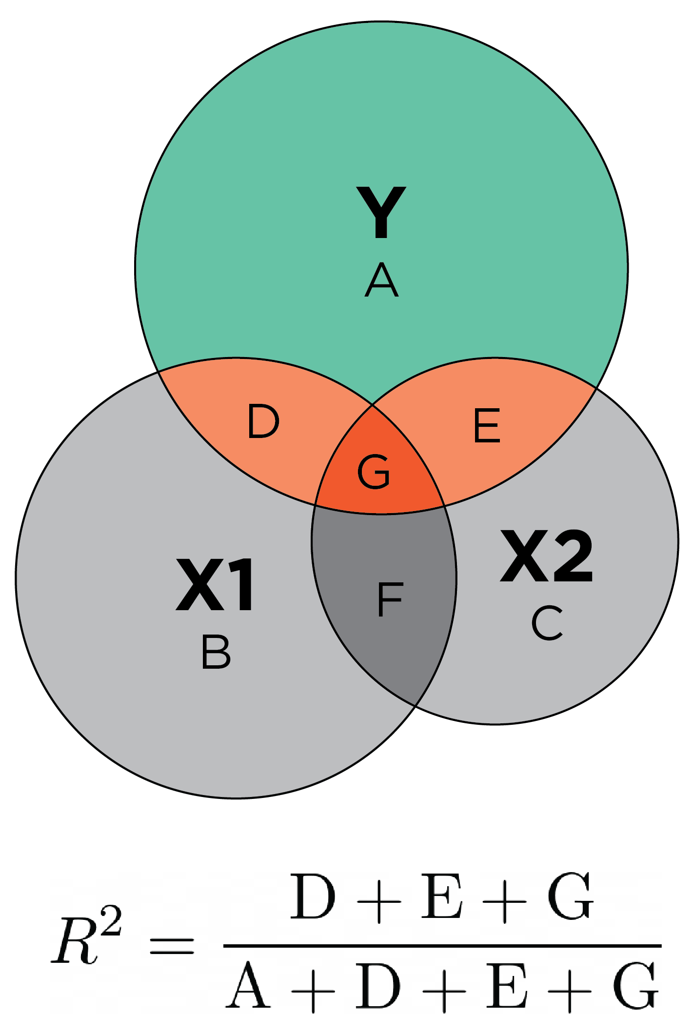
The coefficient of determination (\(R^2\)) is a general index of accuracy that combines both discrimination and calibration. It reflects the proportion of variance in the outcome (dependent) variable that is explained by the model predictions: \(R^2 = \frac{\text{variance explained in }Y}{\text{total variance in }Y}\). Larger values indicate greater accuracy. The formula for the coefficient of determination is in Equation 9.33:
\[ \begin{aligned} R^2 &= 1 - \frac{\sum (y_i - \hat{y}_i)^2}{\sum (y_i - \bar{y})^2} \\ &= 1 - \frac{SS_{\text{residual}}}{SS_{\text{total}}} \\ &= 1 - \frac{\text{sum of squared residuals}}{\text{total sum of squares}} \\ &= \frac{\text{variance explained in }y}{\text{total variance in }y} \end{aligned} \tag{9.33}\]
where \(y\) is the outcome variable, \(y_i\) is the observed value of the outcome variable for the \(i\)th observation, \(\hat{y}_i\) is the model predicted value for the \(i\)th observation, and \(\bar{y}\) is the mean of the observed values of the outcome variable. The total sum of squares is an index of the total variation in the outcome variable.
\(R^2\) is commonly estimated in multiple regression, in which multiple predictors are allowed to predict one outcome. Multiple regression can be conceptualized with overlapping circles in what is called a Ballantine graph (archived at https://perma.cc/C7CU-KFVG). \(R^2\) in multiple regression is depicted conceptually with a Ballantine graph in Figure 9.20.
\(R^2\):
The predictor (testScore) explains \(17.79\)% of the variance \((R^2 = .1779)\) in the outcome (disorder status).
The coefficient of determination typically ranges from 0 to 1, but it can be negative. A negative coefficient of determination indicates that the predicted values are less accurate than using the mean of the actual values as the predicted values (i.e., predicting the mean of the observed values for every case).
An issue with \(R^2\) is that it can be artificially inflated by adding more predictors to the model, even if those predictors do not improve the model fit. \(R^2\) never decreases when adding predictors to a model, even if the predictors do not provide any predictive power. Thus, to account for the number of predictors in the model, we can use adjusted \(R^2\).
9.4.1.2.6.1 Adjusted \(R^2\) (\(R^2_{adj}\))
Adjusted \(R^2\) is similar to the coefficient of determination, but it accounts for the number of predictors included in the regression model to penalize overfitting. Specifically, adjusted \(R^2\) penalizes the number of predictors in the model. Adjusted \(R^2\) reflects the proportion of variance in the outcome (dependent) variable that is explained by the model predictions over and above what would be expected to be accounted for by chance, given the number of predictors in the model. Thus, adjusted \(R^2\) will increase only if the new predictor improves the model (i.e., explains additional variance in the outcome variable) more than would be expected by chance. Larger values indicate greater accuracy. The formula for adjusted \(R^2\) is in Equation 9.34:
\[ R^2_{adj} = 1 - (1 - R^2) \frac{n - 1}{n - p - 1} \tag{9.34}\]
where \(p\) is the number of predictors in the model, and \(n\) is the sample size.
Adjusted \(R^2\) is described further in Section 9.9.
9.4.1.2.6.2 Predictive \(R^2\)
Predictive \(R^2\) is described here: https://tomhopper.me/2014/05/16/can-we-do-better-than-r-squared/ (archived at https://perma.cc/BK8J-HFUK) and https://mfatihtuzen.netlify.app/posts/2025-04-30_rsquared/ (archived at https://perma.cc/EPP8-VG23). Predictive \(R^2\) penalizes overfitting, unlike traditional \(R^2\). Larger values indicate greater accuracy. The formula for predictive \(R^2\) is in Equation 9.35:
\[ R^2_{pred} = 1 - \frac{\text{PRESS}}{\text{SS}_\text{total}} \tag{9.35}\]
where PRESS is the predictive residual sum of squares, and \(\text{SS}_\text{total}\) is the total sum of squares.
Code
#predictive residual sum of squares (PRESS)
PRESS <- function(linear.model) {
  #calculate the predictive residuals
  pr <- residuals(linear.model)/(1-lm.influence(linear.model)$hat)
  #calculate the PRESS
  PRESS <- sum(pr^2)

  return(PRESS)
}

predictiveRSquared <- function(predicted, actual){
  #fit linear model
  linear.model <- lm(actual ~ predicted)

  #use anova() to get the sum of squares for the linear model
  lm.anova <- anova(linear.model)

  #calculate the total sum of squares
  tss <- sum(lm.anova$'Sum Sq')

  #calculate the predictive R^2
  value <- 1 - PRESS(linear.model)/(tss)

  return(value)
}It is preferable to examine predictive \(R^2\) using new data that the model was not trained on—i.e., cross-validation, either in an independent sample (i.e., external cross-validation) or in a hold-out sample (i.e., internal cross-validation on test data).
For example, here is an example of estimating predictive \(R^2\) with 10-fold cross-validation using the caret package (Kuhn, 2022).
Code
set.seed(52242)

# Set up 10-fold cross-validation
train_control <- caret::trainControl(
  method = "cv",
  number = 10)

# Fit the model with cross-validation
model_cv <- caret::train(
  testScore ~ disorder,
  data = mydataSDT,
  method = "lm",
  na.action = na.exclude,
  trControl = train_control,
  metric = "Rsquared")

# View R-squared across the folds
model_cv$results$Rsquared
[1] 0.2727232Here is an example of estimating predictive \(R^2\) with a training and testing data set using the caret package (Kuhn, 2022).
Code
set.seed(52242)

inTrain <- caret::createDataPartition(
  y = as.factor(mydataSDT$disorder),
  p = .75, # the proportion of data for the training data set
  list = FALSE
)

training <- mydataSDT[ inTrain,]
testing  <- mydataSDT[-inTrain,]

training_model <- lm(
  testScore ~ disorder,
  data = training)

testing_predictions <- predict(
  training_model,
  newdata = testing)

accuracyOverall(
  predicted = testing_predictions,
  actual = testing$disorder)$rsquared
[1] 0.44154539.4.2 Discrimination
When dealing with a categorical outcome, discrimination is the ability to separate events from non-events. When dealing with a continuous outcome, discrimination is the strength of the association between the predictor and the outcome. Aspects of discrimination at a particular cutoff (e.g., sensitivity, specificity) are described in Section 9.5.
9.4.2.1 Area under the ROC curve (AUC)
The area under the ROC curve (AUC) is a general index of discrimination accuracy for a categorical outcome. It is also called the concordance (\(c\)) statistic. Larger values reflect greater discrimination accuracy. AUC was estimated using the pROC package (Robin et al., 2021).
9.4.2.2 Coefficient of Predictive Ability (CPA)
The coefficient of predictive ability (CPA) is a generalization of AUC to handle non-binary outcomes including ordinal and continuous outcomes (Gneiting & Walz, 2021). Larger values reflect greater accuracy. It was calculated using the uroc package (Gneiting & Walz, 2021).
9.4.2.3 Spearman’s Rho (\(\rho\)) Rank Correlation
When the coefficient of predictive ability is applied to an ordinal or continuous outcome, it is linearly related to Spearman’s rho (\(\rho\)) rank correlation (Gneiting & Walz, 2021). Larger values reflect greater accuracy. Spearman’s rho was estimated in the rms package (Harrell, Jr., 2021).
9.4.2.4 Somers’ \(D_{xy}\) Rank Correlation
Somers \(D_{xy}\) is an index of discrimination for an ordinal outcome (Harrell, 2015). Larger values reflect greater accuracy. Somers’ \(D_{xy}\) was estimated in the rms package (Harrell, Jr., 2021).
9.4.2.5 Kendall’s Tau-a (\(\tau_A\)) Rank Correlation
Kendall’s tau-a (\(\tau_A\)) is an index of the discrimination for an ordinal outcome (Harrell, 2015). Larger values reflect greater accuracy. Kendall’s tau-a was estimated in the rms package (Harrell, Jr., 2021).
9.4.2.6 \(c\) Index
The \(c\) index, also called the concordance probability, is a generalization of the area under the ROC curve that applies to a continuous outcome (Harrell, 2015). The \(c\) index is the proportion of all pairs of predicted-actual values whose actual value can be ordered such that the pair with the higher predicted value is the one who had the higher actual value. Larger values reflect greater accuracy. The Brown–Hollander–Korwar non-parametric test of association was estimated in the rms package (Harrell, Jr., 2021).
9.4.2.7 Effect Size (\(\beta\)) of Regression
The effect size of a predictor, i.e., the standardized regression coefficient is called a beta (\(\beta\)) coefficient, is a general index of discrimination accuracy for a continuous outcome. Larger values reflect greater accuracy. We can obtain standardized regression coefficients by standardizing the predictors and outcome using the scale() function in R.
\(\beta\):
9.4.3 Calibration
When dealing with a categorical outcome, calibration is the degree to which a probabilistic estimate of an event reflects the true underlying probability of the event. When dealing with a continuous outcome, calibration is the degree to which the predicted values are close in value to the outcome values. The importance of examining calibration (in addition to discrimination) is described by Lindhiem et al. (2020).
Calibration came to be considered a central aspect of weather forecast accuracy. For instance, on the days that the meteorologist says there is a 60% chance of rain, it should rain about 60% of the time. Through improvements in scientific understanding of weather systems, rain forecasts have become more accurate. Meteorologists produce “ensemble forecasts”, where they run many different models (archived at https://perma.cc/248N-9CW5). If all of the models predict a similar outcome (e.g., no rain), the metereologists have greater confidence in the forecast. However, if the models predict different outcomes (e.g., some models predict rain and others predict no rain), the meteorologists have less confidence in the forecast, which is why the meteorologists might predict a “10% chance of rain”.
With these advancements, rain forecasts from the National Weather Service are well calibrated see 9.22. However, forecasts of rain may be exaggerated by local TV meteorologists to boost ratings (Silver, 2012). Interestingly, rain forecasts from The Weather Channel are somewhat miscalibrated under certain conditions. For instance, on days when they forecast a 20% chance of rain, the actual chance of rain is around 5% see 9.21. However, this miscalibration is deliberate. People tend to be more angry when the meteorologist says it will not rain when it actually does (false negative) compared to when the meteorologist says it will rain when it actually does not (false positive). As Silver (2012) notes, “If it rains when it isn’t supposed to, [people] curse the weatherman for ruining their picnic, whereas an unexpectedly sunny day is taken as a serendipitous bonus. It isn’t good science, but as Dr. Rose at The Weather Channel acknowledged to [Mr. Silver]: ‘If the forecast was objective, if it has zero bias in precipitation, we’d probably be in trouble.’” (p. 135).
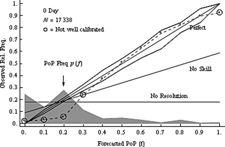
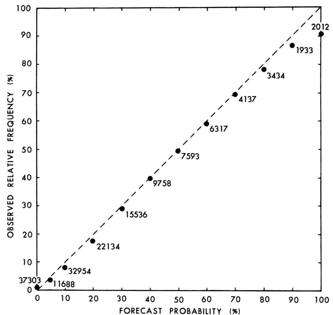
Calibration is not just important for weather forecasts. It is also important for psychological assessment. Calibration can be examined in several ways, including Brier Scores (see Section 9.4.3.2), the Hosler-Lemeshow test (see Section 9.4.3.3), Spiegelhalter’s \(z\) (see Section 9.4.3.4), and the mean difference between predicted and observed values at different binned thresholds as depicted graphically with a calibration plot (see Figure 9.24).
9.4.3.1 Calibration Plot
Calibration plots can be helpful for identifying miscalibration. A calibration plot depicts the predicted probability of an event on the x-axis, and the actual (observed) probability of the event on the y-axis. The predictions are binned into a certain number of groups (commonly 10). The diagonal line reflects predictions that are perfectly calibrated. To the extent that predictions deviate from the diagonal line, the predictions are miscalibrated. There are four general patterns of miscalibration: overextremity, underextremity, overprediction, and underprediction (see Figure 9.23). Overextremity exists when the predicted probabilites are too close to the extremes (zero or one). Underextremity exists when the predicted probabilities are too far away from the extremes. Overprediction exists when the predicted probabilities are consistently greater than the observed probabilities. Underprediction exists when the predicted probabilities are consistently less than the observed probabilities. For a more thorough description of these types of miscalibration, see Lindhiem et al. (2020).
Code
par(mfrow = c(2,2), mar = c(5,4,1,1)+0.1) #margins: bottom, left, top, right
plot(examplePredictions, overExtremity, xlim = c(0,1), ylim = c(0,1), main = "Overextremity", xlab = "Predicted Probability", ylab = "Observed Proportion", bty = "l", cex = 1.5, col = "#e41a1c", type = "o")
lines(c(0,1), c(0,1), lwd = 2, col = "#377eb8")
plot(examplePredictions, underExtremity, xlim = c(0,1), ylim = c(0,1), main = "Underextremity", xlab = "Predicted Probability", ylab = "Observed Proportion", bty = "l", cex = 1.5, col = "#e41a1c", type = "o")
lines(c(0,1), c(0,1), lwd = 2, col = "#377eb8")
plot(examplePredictions, overPrediction, xlim = c(0,1), ylim = c(0,1), main = "Overprediction", xlab = "Predicted Probability", ylab = "Observed Proportion", bty = "l", cex = 1.5, col = "#e41a1c", type = "o")
lines(c(0,1), c(0,1), lwd = 2, col = "#377eb8")
plot(examplePredictions, underPrediction, xlim = c(0,1), ylim = c(0,1), main = "Underprediction", xlab = "Predicted Probability", ylab = "Observed Proportion", bty = "l", cex = 1.5, col = "#e41a1c", type = "o")
lines(c(0,1), c(0,1), lwd = 2, col = "#377eb8")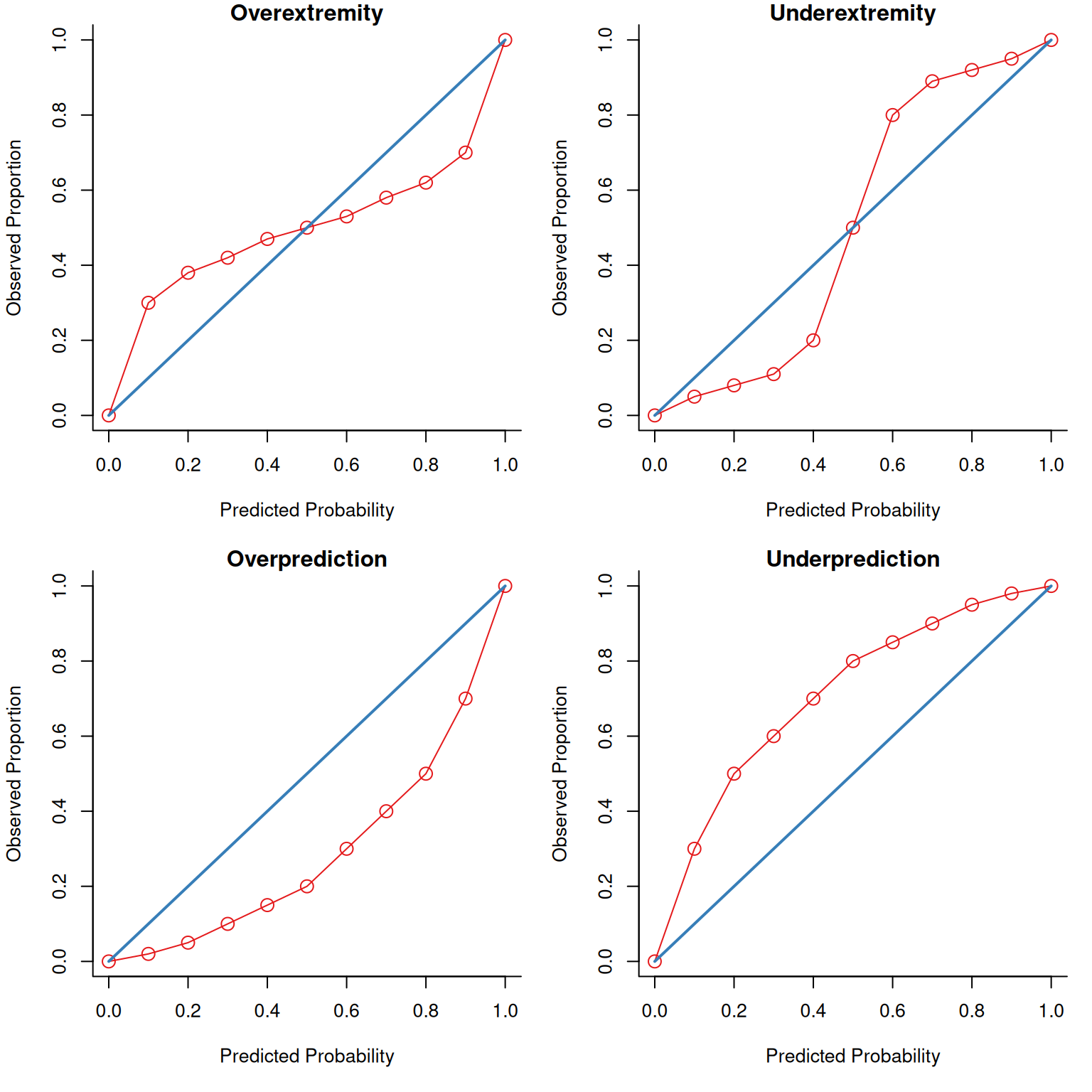
This calibration plot was generated using the PredictABEL package (Kundu et al., 2020), and is depicted in Figure 9.24.
Code
$Table_HLtest
                total meanpred meanobs predicted observed
[0.0000,0.0245)    19    0.013   0.211      0.25        4
0.0245              7    0.025   0.143      0.17        1
0.0294              8    0.029   0.250      0.24        2
[0.0343,0.0441)    13    0.036   0.231      0.47        3
[0.0441,0.0588)    10    0.051   0.300      0.51        3
[0.0588,0.0735)    10    0.063   0.100      0.63        1
[0.0735,0.1324)    10    0.099   0.500      0.99        5
[0.1324,0.2059)    12    0.165   0.583      1.98        7
[0.2059,0.2598)    10    0.222   0.300      2.22        3
[0.2598,1.0000]    11    0.408   1.000      4.49       11

$Chi_square
[1] 152.274

$df
[1] 8

$p_value
[1] 0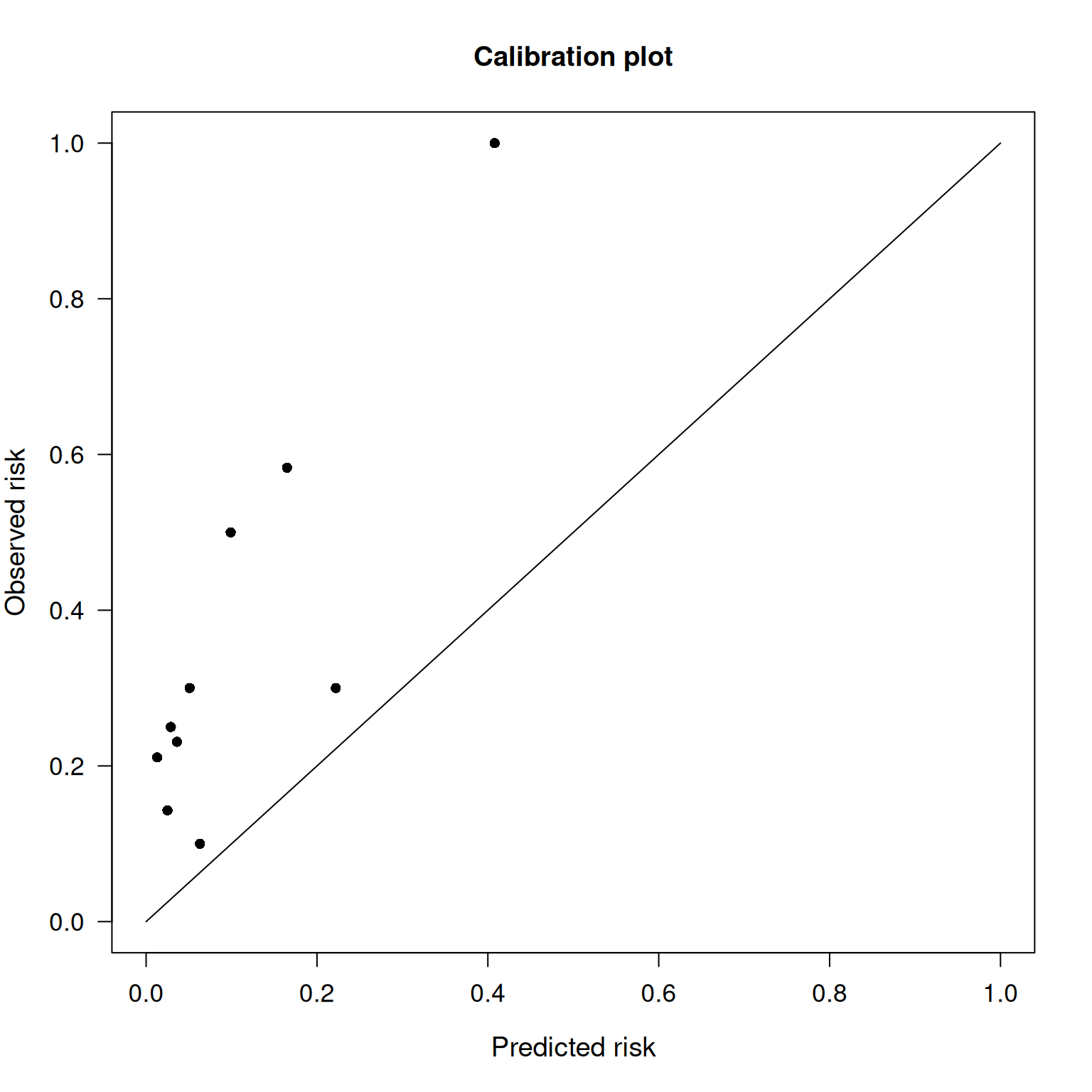
This calibration plot (and ROC curve) was generated using the rms package (Harrell, Jr., 2021), and is depicted in Figure 9.25. The calibration plot is consistent with underprediction. That is, the predicted probabilities were consistently lower than the actual probabilities. To re-calibrate the predicted probabilities, it would be necessary to increase them so they are consistent with observed probabilties.
          Dxy       C (ROC)            R2             D      D:Chi-sq
 4.769231e-01  7.384615e-01 -6.156954e-01 -3.797827e-01 -4.039632e+01
          D:p             U      U:Chi-sq           U:p             Q
 1.000000e+00           Inf           Inf  0.000000e+00          -Inf
        Brier     Intercept         Slope          Emax           E90
 2.659086e-01  1.682881e+00  8.857501e-01  7.146778e-01  3.719585e-01
         Eavg           S:z           S:p
2.618115e-01 1.052663e+01 6.512514e-26 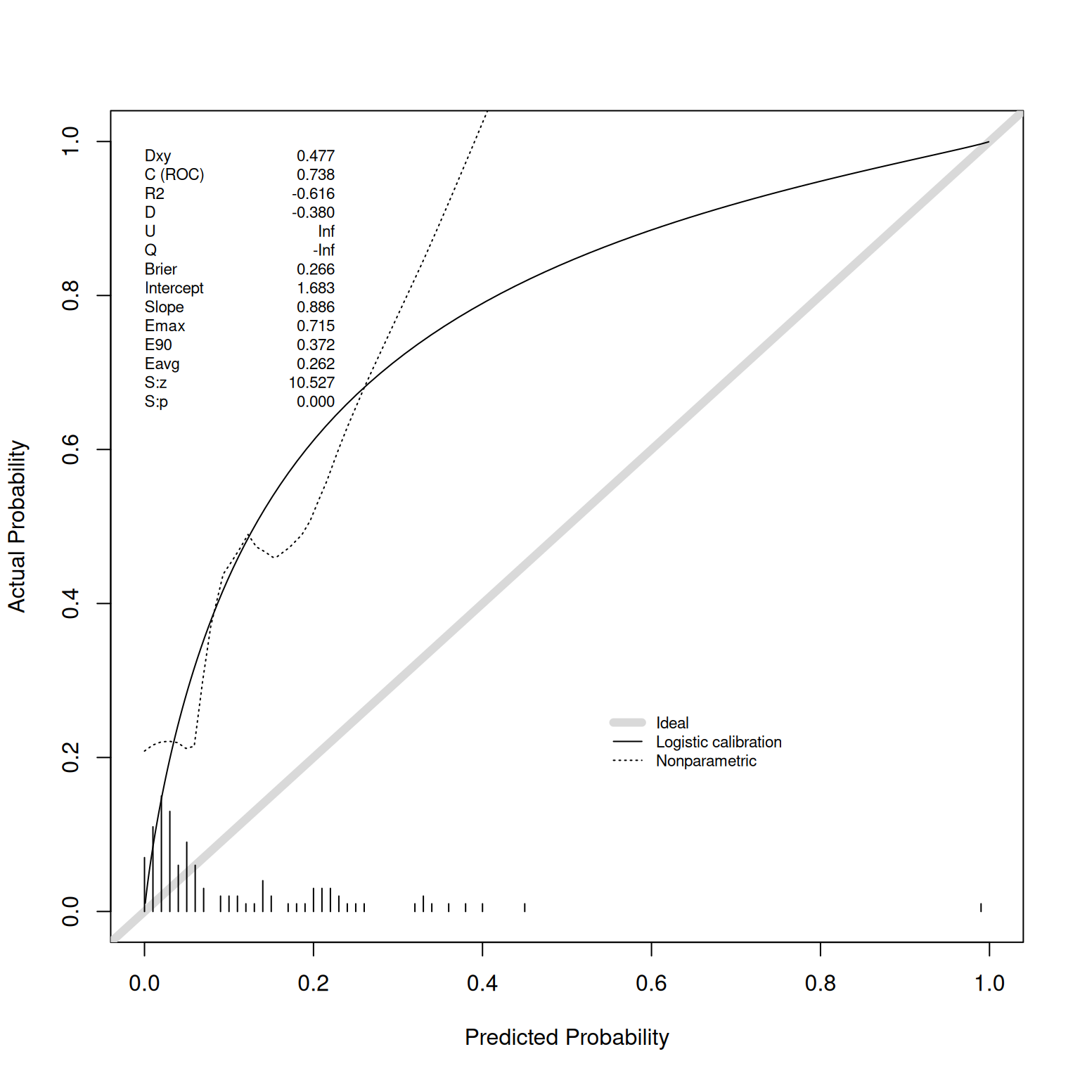
This calibration plot was adapted from Darren Dahly’s example, and is depicted in Figure 9.26: https://darrendahly.github.io/post/homr/ (archived at https://perma.cc/6J3J-69G7)
Code
g1 <- mutate(mydataSDT, bin = cut_number(predictedProbability, 10)) %>%
  # Bin prediction into 10ths
  group_by(bin) %>%
  mutate(n = length(na.omit(predictedProbability)), # Get ests and CIs
         bin_pred = mean(predictedProbability, na.rm = TRUE),
         bin_prob = mean(disorder, na.rm = TRUE),
         se = sd(disorder, na.rm = TRUE) / sqrt(n),
         ul = bin_prob + qnorm(.975) * se,
         ll = bin_prob - qnorm(.975) * se) %>%
  ungroup() %>%
  ggplot(aes(x = bin_pred, y = bin_prob, ymin = ll, ymax = ul)) +
  geom_pointrange(size = 0.5, color = "black") +
  scale_y_continuous(limits = c(0, 1), breaks = seq(0, 1, by = 0.1)) +
  scale_x_continuous(limits = c(0, 1), breaks = seq(0, 1, by = 0.1)) +
  geom_abline() + # 45 degree line indicating perfect calibration
  geom_smooth(method = "lm", se = FALSE, linetype = "dashed",
              color = "black", formula = y~-1 + x) +
  # straight line fit through estimates
  geom_smooth(aes(x = predictedProbability, y = disorder),
              color = "red", se = FALSE, method = "loess") +
  # loess fit through estimates
  xlab("") +
  ylab("Observed Probability") +
  theme_minimal()+
  xlab("Predicted Probability")

g2 <- ggplot(mydataSDT, aes(x = predictedProbability)) +
  geom_histogram(fill = "black", bins = 200) +
  scale_x_continuous(limits = c(0, 1), breaks = seq(0, 1, by = 0.1)) +
  xlab("Histogram of Predicted Probability") +
  ylab("") +
  theme_minimal() +
  theme(panel.grid.minor = element_blank())

g <- arrangeGrob(g1, g2, respect = TRUE, heights = c(1, 0.25), ncol = 1)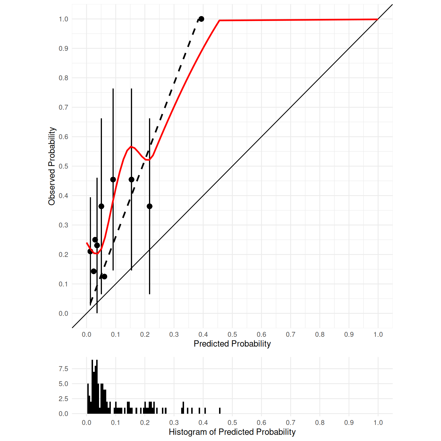
9.4.3.2 Brier Scores
Brier scores were calculated using the rms package (Harrell, Jr., 2021). Smaller values reflect greater calibration accuracy.
9.4.3.3 Hosler-Lemeshow Test
The Hosler-Lemeshow goodness of fit (GOF) test evaluates the null hypothesis that there is no difference between the predicted versus observed frequencies of an event. The test requires specifying how many groups/bins (\(g\)) to use to calculate quantiles. Smaller \(\chi^2\) values (and larger p-values) reflect greater calibration accuracy. A statistically significant \(\chi^2\) (p < .05) indicates a significant degree of miscalibration. The Hosler-Lemeshow GOF test was calculated using the ResourceSelection package (Lele et al., 2019). The table of predicted versus observed frequencies was generated using the PredictABEL package (Kundu et al., 2020).
For each number of bins (\(g\)) specified below, the predictions show statistically significant miscalibration.
\(g = 2\)
    Hosmer and Lemeshow goodness of fit (GOF) test

data:  mydataSDT$disorder, mydataSDT$predictedProbability
X-squared = NA, df = 0, p-value = NA
Code
                total meanpred meanobs predicted observed
[0.0000,0.0588)    57    0.029   0.228      1.64       13
[0.0588,1.0000]    53    0.194   0.509     10.29       27
\(g = 4\)
    Hosmer and Lemeshow goodness of fit (GOF) test

data:  mydataSDT$disorder, mydataSDT$predictedProbability
X-squared = NA, df = 2, p-value = NA
Code
                total meanpred meanobs predicted observed
[0.0000,0.0343)    34    0.019   0.206      0.66        7
[0.0343,0.0588)    23    0.043   0.261      0.98        6
[0.0588,0.1569)    26    0.095   0.346      2.48        9
[0.1569,1.0000]    27    0.289   0.667      7.81       18
\(g = 6\)
    Hosmer and Lemeshow goodness of fit (GOF) test

data:  mydataSDT$disorder, mydataSDT$predictedProbability
X-squared = NA, df = 4, p-value = NA
Code
                total meanpred meanobs predicted observed
[0.0000,0.0245)    19    0.013   0.211      0.25        4
[0.0245,0.0392)    23    0.030   0.217      0.68        5
[0.0392,0.0588)    15    0.047   0.267      0.71        4
[0.0588,0.1127)    17    0.074   0.235      1.26        4
[0.1127,0.2206)    19    0.167   0.474      3.18        9
[0.2206,1.0000]    17    0.344   0.824      5.85       14
\(g = 8\)
    Hosmer and Lemeshow goodness of fit (GOF) test

data:  mydataSDT$disorder, mydataSDT$predictedProbability
X-squared = NA, df = 6, p-value = NA
Code
                total meanpred meanobs predicted observed
[0.0000,0.0245)    19    0.013   0.211      0.25        4
[0.0245,0.0343)    15    0.027   0.200      0.41        3
0.0343              8    0.034   0.250      0.27        2
[0.0392,0.0588)    15    0.047   0.267      0.71        4
[0.0588,0.0931)    13    0.066   0.077      0.86        1
[0.0931,0.1569)    13    0.124   0.615      1.62        8
[0.1569,0.2402)    15    0.206   0.400      3.09        6
[0.2402,1.0000]    12    0.394   1.000      4.73       12
\(g = 10\)
    Hosmer and Lemeshow goodness of fit (GOF) test

data:  mydataSDT$disorder, mydataSDT$predictedProbability
X-squared = NA, df = 8, p-value = NA
Code
                total meanpred meanobs predicted observed
[0.0000,0.0245)    19    0.013   0.211      0.25        4
0.0245              7    0.025   0.143      0.17        1
0.0294              8    0.029   0.250      0.24        2
[0.0343,0.0441)    13    0.036   0.231      0.47        3
[0.0441,0.0588)    10    0.051   0.300      0.51        3
[0.0588,0.0735)    10    0.063   0.100      0.63        1
[0.0735,0.1324)    10    0.099   0.500      0.99        5
[0.1324,0.2059)    12    0.165   0.583      1.98        7
[0.2059,0.2598)    10    0.222   0.300      2.22        3
[0.2598,1.0000]    11    0.408   1.000      4.49       11
9.4.3.4 Spiegelhalter’s z
Spiegelhalter’s \(z\) was calculated using the rms package (Harrell, Jr., 2021). Smaller \(z\) values (and larger associated \(p\)-values) reflect greater calibration accuracy. A statistically significant Spiegelhalter’s \(z\) (p < .05) indicates a significant degree of miscalibration.
In this case, the predictions show statistically significant miscalibration.
9.4.3.5 Calibration for predicting a continuous outcome
When predicting a continuous outcome, calibration of the predicted values in relation to the outcome values can be examined in multiple ways including:
- in a calibration plot, the extent to which the intercept is near zero and the slope is near one
- in a calibration plot, the extent to which the 95% confidence interval of the observed value, across all values of the predicted values, includes the diagonal reference line with an intercept of zero and a slope of one.
- mean error
- mean absolute error
- mean squared error
- root mean squared error
With a plot of the predictions on the x-axis, and the outcomes on the y-axis (i.e., a calibration plot), calibration can be examined graphically as the extent to which the best-fit regression line has an intercept (alpha) close to zero and a slope (beta) close to one (Stevens & Poppe, 2020; Steyerberg & Vergouwe, 2014). The intercept is also called “calibration-in-the-large”, whereas “calibration-in-the-small” refers to the extent to which the predicted values match the observed values at a specific predicted value (e.g., when the weather forecaster says that there is a 10% chance of rain, does it actually rain 10% of the time?). For predictions to be well calibrated, the intercept should be close to zero and the slope should be close to one. If the slope is close to one but the intercept is not close to zero (or the intercept is close to zero but the slope is not close to one), the predictions would not be considered well calibrated. The 95% confidence interval of the observed value, across all values of the predicted values, should include the diagonal reference line whose intercept is zero and whose slope is one.
For instance, based on the intercept and slope of the calibration plot in Figure 9.27, the predictions are not well calibrated, despite having a slope near one, because the 95% confidence interval of the intercept does not include zero. The best-fit line is the yellow line. The intercept from the best-fit line is positive, as shown in the regression equation. This is a case of underprediction, where the predicted values are consistently less than the observed values. The confidence interval of the observed value (i.e., the purple band) is the interval within which we have 95% confidence that the true observed value would lie for a given predicted value, based on the model. The 95% prediction interval of the observed value (i.e., the dashed red lines) is the interval within which we would expect that 95% of future observations would lie for a given predicted value. The black diagonal line indicates the reference line with an intercept of zero and a slope of one. The predictions would be significantly miscalibrated at a given level of the predicted values if the 95% confidence interval of the observed value does not include the reference line at that level of the predicted value. In this case, the 95% confidence interval of the observed value does not include the reference line (i.e., the actual observed value) at lower levels of the predicted values, so the predictions are miscalibrated lower levels of the predicted values.
Code
#95 prediction interval based on linear model
calibrationModel <- lm(
  continuousOutcome ~ testScore,
  data = mydataSDT)
calibrationModelPredictionInterval <- expand.grid(
  testScore = seq(from = min(mydataSDT$testScore, na.rm = TRUE),
                  to = max(mydataSDT$testScore, na.rm = TRUE),
                  length.out = 1000))
calibrationModelPredictionInterval <- cbind(
  calibrationModelPredictionInterval,
  data.frame(predict(
    calibrationModel,
    newdata = calibrationModelPredictionInterval,
    interval = "predict",
    level = 0.95)))

ggplot(
  mydataSDT,
  aes(
    x = testScore,
    y = continuousOutcome)) +
  geom_point() +
  geom_line(
    data = calibrationModelPredictionInterval,
    aes(y = lwr),
    color = "red",
    linetype = "dashed") + #Lower estimate of 95% prediction interval of linear model
  geom_line(
    data = calibrationModelPredictionInterval,
    aes(y = upr),
    color = "red",
    linetype = "dashed") + #Upper estimate of 95% prediction interval of linear model
  #geom_ribbon(data = calibrationModelPredictionInterval, aes(y = fit, ymin = lwr, ymax = upr), fill = viridis(3)[1], alpha = 0.7) + #95% prediction interval of linear model
  geom_smooth(
    method = "lm",
    color = viridis(3)[3], fill = viridis(3)[1],
    alpha = 0.7) + #95% confidence interval of linear model
  geom_abline(
    slope = 1,
    intercept = 0) +
  xlim(0,2.4) +
  ylim(0,2.4) +
  xlab("Predicted Value") +
  ylab("Observed Value") +
  stat_cor(
    label.y = 2.2,
    aes(label = paste(..rr.label..))) +
  stat_regline_equation(label.y = 2.0) +
  theme_bw()
Gold-standard recommendations include examining the predicted values in relation to the observed values using locally estimated scatterplot smoothing (LOESS) (Austin & Steyerberg, 2014), such as in Figure 9.28. We can examine whether the LOESS-based 95% confidence interval of the observed value at every level of the predicted values includes the diagonal reference line (i.e., the actual observed value). In this case, the 95% confidence interval of the observed value does not include the reference line at lower levels of the predicted values, so the predictions are miscalibrated at lower levels of the predicted values.
(ref:calibrationContinuousOutcomeLOESSCaption) Calibration Plot for Predictions of a Continuous Outcome, With LOESS Best-Fit Line. The yellow line is the best-fit line based on LOESS. The purple band is the 95% confidence interval of the observed value. The dashed red lines are the 95% prediction interval of the observed value. The 95% confidence interval of the observed value does not include the reference line (i.e., the actual observed value) at lower levels of the predicted values, so the predictions are miscalibrated at lower levels of the predicted values.
Code
#95 prediction interval based on LOESS model
calibrationLoessModel <- loess.sd(
  x = mydataSDT$testScore,
  y = mydataSDT$continuousOutcome,
  nsigma = qnorm(.975),
  na.action = "na.exclude")
calibrationLoessPredictionInterval <- data.frame(
  x = calibrationLoessModel$x,
  y = calibrationLoessModel$y,
  lower = calibrationLoessModel$lower,
  upper = calibrationLoessModel$upper)

ggplot(
  mydataSDT,
  aes(
    x = testScore,
    y = continuousOutcome)) +
  geom_point() +
  geom_line(
    data = calibrationLoessPredictionInterval,
    aes(x = x, y = lower),
    color = "red",
    linetype = "dashed") + #Lower estimate of 95% prediction interval of linear model
  geom_line(
    data = calibrationLoessPredictionInterval,
    aes(x = x, y = upper),
    color = "red",
    linetype = "dashed") + #Upper estimate of 95% prediction interval of linear model
  #geom_ribbon(data = calibrationLoessPredictionInterval, aes(x = x, y = y, ymin = lower, ymax = upper), fill = viridis(3)[1], alpha = 0.7) + #95% prediction interval of linear model
  geom_smooth(
    method = "loess",
    color = viridis(3)[3], fill = viridis(3)[1],
    alpha = 0.7) + #95% confidence interval of LOESS model
  geom_abline(
    slope = 1,
    intercept = 0) +
  xlim(0,2.4) +
  ylim(0,2.4) +
  xlab("Predicted Value") +
  ylab("Observed Value") +
  theme_bw()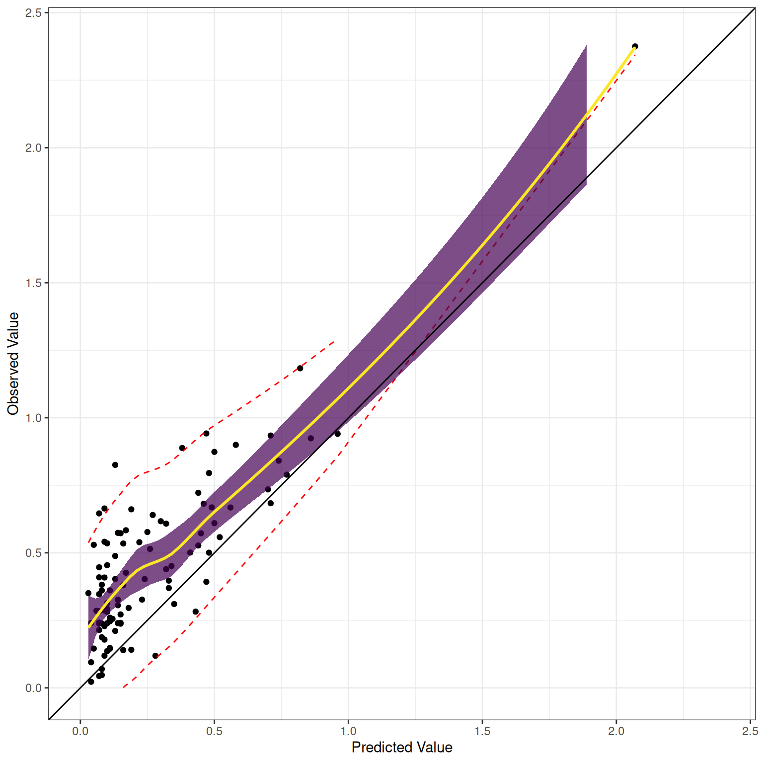
9.5 Prediction Accuracy at a Given Cutoff
9.5.1 Set a Cutoff
Here, I set a cutoff at the Youden’s J Statistic to calculate the accuracy statistics at that cutoff:
Code
cutoff <- 0.205

mydataSDT$diagnosis <- NA
mydataSDT$diagnosis[mydataSDT$testScore < cutoff] <- 0
mydataSDT$diagnosis[mydataSDT$testScore >= cutoff] <- 1

mydataSDT$diagnosisFactor <- factor(
  mydataSDT$diagnosis,
  levels = c(1, 0),
  labels = c("Decision: Diagnosis", "Decision: No Diagnosis"))

mydataSDT$disorderFactor <- factor(
  mydataSDT$disorder,
  levels = c(1, 0),
  labels = c("Truth: Disorder", "Truth: No Disorder"))
9.5.2 Accuracy at a Given Cutoff
The petersenlab package (Petersen, 2025) contains the accuracyAtCutoff() function that estimates the prediction accuracy at a given cutoff.
Code
                                               [,1]
cutoff                                         0.20
TP                                            26.00
TN                                            56.00
FP                                            14.00
FN                                            14.00
SR                                             0.36
BR                                             0.36
percentAccuracy                               74.55
percentAccuracyByChance                       53.72
percentAccuracyPredictingFromBaseRate         63.64
RIOC                                           0.45
relativeImprovementOverPredictingFromBaseRate  0.15
SN                                             0.65
SP                                             0.80
TPrate                                         0.65
TNrate                                         0.80
FNrate                                         0.35
FPrate                                         0.20
HR                                             0.65
FAR                                            0.20
PPV                                            0.65
NPV                                            0.80
FDR                                            0.35
FOR                                            0.20
youdenJ                                        0.45
balancedAccuracy                               0.73
f1Score                                        0.65
mcc                                            0.45
diagnosticOddsRatio                            7.43
positiveLikelihoodRatio                        3.25
negativeLikelihoodRatio                        0.44
dPrimeSDT                                      1.23
betaSDT                                        1.32
cSDT                                           0.23
aSDT                                           0.79
bSDT                                           1.33
informationGain                                0.15
differenceBetweenPredictedAndObserved         -0.27
There are also test calculators available online:
9.5.3 Confusion Matrix aka 2x2 Accuracy Table aka Cross-Tabulation aka Contingency Table
A confusion matrix (aka 2x2 accuracy table, cross-tabulation table, or contigency table) is a matrix for categorical data that presents the predicted outcome on one dimension and the actual outcome (truth) on the other dimension. If the predictions and outcomes are dichotomous, the confusion matrix is a 2x2 matrix with two rows and two columns that represent four possible predicted-actual combinations (decision outcomes). In such a case, the confusion matrix provides a tabular count of each type of accurate cases (true positives and true negatives) versus the number of each type of error (false positives and false negatives), as shown in Figure 9.29. An example of a confusion matrix is in Figure 9.4.
.](images/confusionMatrix.png)
9.5.3.1 Number
9.5.3.2 Number with margins added
9.5.3.3 Proportions
9.5.3.4 Proportions with margins added
9.5.4 True Positives (TP)
True positives (TPs) are instances in which a positive classification (e.g., a disorder present) is correct—that is, the test says that a classification is present, and the classification is present. True positives are also called valid positives (VPs) or hits. Higher values (relative to the same sample size) reflect greater accuracy. The formula for true positives is in Equation 9.36:
\[ \begin{aligned} \text{TP} &= \text{BR} \times \text{SR} \times N \end{aligned} \tag{9.36}\]
9.5.5 True Negatives (TN)
True negatives (TNs) are instances in which a negative classification (e.g., absence of a disorder) is correct—that is, the test says that a classification is not present, and the classification is actually not present. True negatives are also called valid negatives (VNs) or correct rejections. Higher values (relative to the same sample size) reflect greater accuracy. The formula for true negatives is in Equation 9.37:
\[ \begin{aligned} \text{TN} &= (1 - \text{BR}) \times (1 - \text{SR}) \times N \end{aligned} \tag{9.37}\]
9.5.6 False Positives (FP)
False positives (FPs) are instances in which a positive classification (e.g., a disorder present) is incorrect—that is, the test says that a classification is present, and the classification is not present. False positives are also called false alarms (FAs). Lower values (relative to the same sample size) reflect greater accuracy. The formula for false positives is in Equation 9.38:
\[ \begin{aligned} \text{FP} &= (1 - \text{BR}) \times \text{SR} \times N \end{aligned} \tag{9.38}\]
9.5.7 False Negatives (FN)
False negatives (FNs) are instances in which a negative classification (e.g., absence of a disorder) is incorrect—that is, the test says that a classification is not present, and the classification is present. False negatives are also called misses. Lower values (relative to the same sample size) reflect greater accuracy. The formula for false negatives is in Equation 9.39:
\[ \begin{aligned} \text{FN} &= \text{BR} \times (1 - \text{SR}) \times N \end{aligned} \tag{9.39}\]
9.5.8 Sample Size (N)
9.5.9 Selection Ratio (SR)
The selection ratio (SR) is the marginal probability of selection, independent of other things: \(P(R_i)\). In clinical psychology, the selection ratio is the proportion of people who test positive for the disorder, as in Equation 9.40:
\[ \begin{aligned} \text{SR} &= P(R_i) \\ &= \frac{\text{TP} + \text{FP}}{N} \end{aligned} \tag{9.40}\]
9.5.10 Base Rate (BR)
The base rate (BR) of a classification is its marginal probability, independent of other things: \(P(C_i)\). In clinical psychology, the base rate of a disorder is its prevalence in the population, as in Equation 9.41. Without additional information, the base rate is used as the initial pretest probability.
\[ \begin{aligned} \text{BR} &= P(C_i) \\ &= \frac{\text{TP} + \text{FN}}{N} \end{aligned} \tag{9.41}\]
9.5.11 Pretest Odds
The pretest odds of a classification can be estimated using the pretest probability (i.e., base rate). To convert a probability to odds, divide the probability by one minus that probability, as in Equation 9.42.
\[ \begin{aligned} \text{pretest odds} &= \frac{\text{pretest probability}}{1 - \text{pretest probability}} \\ \end{aligned} \tag{9.42}\]
9.5.12 Percent Accuracy
Percent Accuracy is also called overall accuracy. Higher values reflect greater accuracy. The formula for percent accuracy is in Equation 9.43. Percent accuracy has several problems. First, it treats all errors (FP and FN) as equally important. However, in practice, it is rarely the case that false positives and false negatives are equally important. Second, percent accuracy can be misleading because it is highly influenced by base rates. You can have a high percent accuracy by predicting from the base rate and saying that no one has the characteristic (if the base rate is low) or that everyone has the characteristic (if the base rate is high). Thus, it is also important to consider other aspects of accuracy.
\[ \text{Percent Accuracy} = 100\% \times \frac{\text{TP} + \text{TN}}{N} \tag{9.43}\]
9.5.13 Percent Accuracy by Chance
The formula for calculating percent accuracy by chance is in Equation 9.44.
\[ \begin{aligned} \text{Percent Accuracy by Chance} &= 100\% \times [P(\text{TP}) + P(\text{TN})] \\ &= 100\% \times \{(\text{BR} \times {\text{SR}}) + [(1 - \text{BR}) \times (1 - \text{SR})]\} \end{aligned} \tag{9.44}\]
9.5.14 Percent Accuracy Predicting from the Base Rate
Predicting from the base rate is going with the most likely outcome in every prediction. It is also called “betting from the base rate”. If the base rate is less than .50, it would involve predicting that the condition is absent for every case. If the base rate is .50 or above, it would involve predicting that the condition is present for every case. Predicting from the base rate is a special case of percent accuracy by chance when the selection ratio is set to either one (if the base rate \(\geq\) .5) or zero (if the base rate < .5).
9.5.15 Relative Improvement Over Chance (RIOC)
Relative improvement over chance (RIOC) is a prediction’s improvement over chance as a proportion of the maximum possible improvement over chance, as described by Farrington & Loeber (1989). Higher values reflect greater accuracy. The formula for calculating RIOC is in Equation 9.45.
\[ \begin{aligned} \text{relative improvement over chance (RIOC)} &= \frac{\text{total correct} - \text{chance correct}}{\text{maximum correct} - \text{chance correct}} \\ \end{aligned} \tag{9.45}\]
Code
relativeImprovementOverChance <- function(TP, TN, FP, FN){
  N <- TP + TN + FP + FN
  actualYes <- TP + FN
  predictedYes <- TP + FP
  value <- ((N * (TP + TN)) - (actualYes * predictedYes + (N - predictedYes) * (N - actualYes))) / ((N * (actualYes + N - predictedYes)) - (actualYes * predictedYes + (N - predictedYes) * (N - actualYes)))

  return(value)
}9.5.16 Relative Improvement Over Predicting from the Base Rate
Relative improvement over predicting from the base rate is a prediction’s improvement over predicting from the base rate as a proportion of the maximum possible improvement over predicting from the base rate. Higher values reflect greater accuracy. The formula for calculating relative improvement over predicting from the base rate is in Equation 9.46.
\[ \scriptsize \begin{aligned} \text{relative improvement over predicting from base rate} &= \frac{\text{total correct} - \text{correct by predicting from base rate}}{\text{maximum correct} - \text{correct by predicting from base rate}} \\ \end{aligned} \tag{9.46}\]
Code
relativeImprovementOverPredictingFromBaseRate <- function(TP, TN, FP, FN){
  N <- TP + TN + FP + FN
  BR <- (TP + FN)/N

  ifelse(BR >= .5, SR <- 1, NA)
  ifelse(BR < .5, SR <- 0, NA)

  actualYes <- TP + FN
  predictedYes <- SR * N
  value <- ((N * (TP + TN)) - (actualYes * predictedYes + (N - predictedYes) * (N - actualYes))) / ((N * (actualYes + N - predictedYes)) - (actualYes * predictedYes + (N - predictedYes) * (N - actualYes)))

  return(value)
}9.5.17 Sensitivity (SN)
Sensitivity (SN) is also called true positive rate (TPR), hit rate (HR), or recall. Sensitivity is the conditional probability of a positive test given that the person has the condition: \(P(R|C)\). Higher values reflect greater accuracy. The formula for calculating sensitivity is in Equation 9.47. As described in Section 9.1.2.6.1 and as depicted in Figure 9.30, as the cutoff increases (becomes more conservative), sensitivity decreases. As the cutoff decreases, sensitivity increases.
\[ \begin{aligned} \text{sensitivity (SN)} &= P(R|C) \\ &= \frac{\text{TP}}{\text{TP} + \text{FN}} = \frac{\text{TP}}{N \times \text{BR}} = 1 - \text{FNR} \end{aligned} \tag{9.47}\]
Below I compute sensitivity and specificity at every possible cutoff.
Code
possibleCutoffs <- unique(na.omit(mydataSDT$testScore))
possibleCutoffs <- possibleCutoffs[order(possibleCutoffs)]
possibleCutoffs <- c(
  possibleCutoffs,
  max(possibleCutoffs, na.rm = TRUE) + 0.01)

specificity <- function(TP, TN, FP, FN){
  value <- TN/(TN + FP)

  return(value)
}

accuracyVariables <- c("cutoff", "TP", "TN", "FP", "FN")

accuracyStats <- data.frame(matrix(
  nrow = length(possibleCutoffs),
  ncol = length(accuracyVariables)))

names(accuracyStats) <- accuracyVariables

for(i in 1:length(possibleCutoffs)){
  newCutoff <- possibleCutoffs[i]

  mydataSDT$diagnosis <- NA
  mydataSDT$diagnosis[mydataSDT$testScore < newCutoff] <- 0
  mydataSDT$diagnosis[mydataSDT$testScore >= newCutoff] <- 1

  accuracyStats[i, "cutoff"] <- newCutoff
  accuracyStats[i, "TP"] <- length(which(
    mydataSDT$diagnosis == 1 & mydataSDT$disorder == 1))
  accuracyStats[i, "TN"] <- length(which(
    mydataSDT$diagnosis == 0 & mydataSDT$disorder == 0))
  accuracyStats[i, "FP"] <- length(which(
    mydataSDT$diagnosis == 1 & mydataSDT$disorder == 0))
  accuracyStats[i, "FN"] <- length(which(
    mydataSDT$diagnosis == 0 & mydataSDT$disorder == 1))
}

accuracyStats$sensitivity <- accuracyStats$TPrate <- sensitivity(
  TP = accuracyStats$TP,
  TN = accuracyStats$TN,
  FP = accuracyStats$FP,
  FN = accuracyStats$FN)

accuracyStats$specificity <- accuracyStats$TNrate <- specificity(
  TP = accuracyStats$TP,
  TN = accuracyStats$TN,
  FP = accuracyStats$FP,
  FN = accuracyStats$FN)

sensitivitySpecificityData <- pivot_longer(
  accuracyStats,
  cols = all_of(c("sensitivity","specificity")))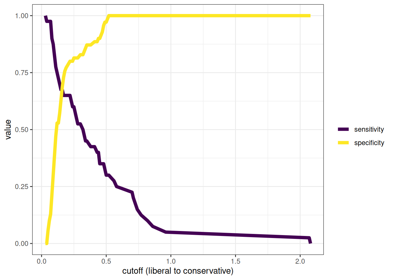
9.5.18 Specificity (SP)
Specificity (SP) is also called true negative rate (TNR) or selectivity. Specificity is the conditional probability of a negative test given that the person does not have the condition: \(P(\text{not } R|\text{not } C)\). Higher values reflect greater accuracy. The formula for calculating specificity is in Equation 9.48. As described in Section 9.1.2.6.1 and as depicted in Figure 9.30, as the cutoff increases (becomes more conservative), specificity increases. As the cutoff decreases, specificity decreases.
\[ \begin{aligned} \text{specificity (SP)} &= P(\text{not } R|\text{not } C) \\ &= \frac{\text{TN}}{\text{TN} + \text{FP}} = \frac{\text{TN}}{N (1 - \text{BR})} = 1 - \text{FPR} \end{aligned} \tag{9.48}\]
9.5.19 False Negative Rate (FNR)
The false negative rate (FNR) is also called the miss rate. The false negative rate is the conditional probability of a negative test given that the person has the condition: \(P(\text{not } R|C)\). Lower values reflect greater accuracy. The formula for calculating false negative rate is in Equation 9.49.
\[ \begin{aligned} \text{false negative rate (FNR)} &= P(\text{not } R|C) \\ &= \frac{\text{FN}}{\text{FN} + \text{TP}} = \frac{\text{FN}}{N \times \text{BR}} = 1 - \text{TPR} \end{aligned} \tag{9.49}\]
9.5.20 False Positive Rate (FPR)
The false positive rate (FPR) is also called the false alarm rate (FAR) or fall-out. The false positive rate is the conditional probability of a positive test given that the person does not have the condition: \(P(R|\text{not } C)\). Lower values reflect greater accuracy. The formula for calculating false positive rate is in Equation 9.50.
\[ \begin{aligned} \text{false positive rate (FPR)} &= P(R|\text{not } C) \\ &= \frac{\text{FP}}{\text{FP} + \text{TN}} = \frac{\text{FP}}{N (1 - \text{BR})} = 1 - \text{TNR} \end{aligned} \tag{9.50}\]
9.5.21 Positive Predictive Value (PPV)
The positive predictive value (PPV) is also called the positive predictive power (PPP) or precision. Many people confuse sensitivity (\(P(R|C)\)) with its inverse conditional probability, PPV (\(P(C|R)\)). PPV is the conditional probability of having the condition given a positive test: \(P(C|R)\). Higher values reflect greater accuracy. The formula for calculating positive predictive value is in Equation 9.51.
PPV can be low even when sensitivity is high because it depends not only on sensitivity, but also on specificity and the base rate. Because PPV depends on the base rate, PPV is not an intrinsic property of a measure. The same measure will have a different PPV in different contexts with different base rates (Treat & Viken, 2023). As described in Section 9.1.2.6.1 and as depicted in Figure 9.31, as the base rate increases, PPV increases. As the base rate decreases, PPV decreases. PPV also differs as a function of the cutoff. As described in Section 9.1.2.6.1 and as depicted in Figure 9.32, as the cutoff increases (becomes more conservative), PPV increases. As the cutoff decreases (becomes more liberal), PPV decreases.
\[ \small \begin{aligned} \text{positive predictive value (PPV)} &= P(C|R) \\ &= \frac{\text{TP}}{\text{TP} + \text{FP}} = \frac{\text{TP}}{N \times \text{SR}}\\ &= \frac{\text{sensitivity} \times {\text{BR}}}{\text{sensitivity} \times {\text{BR}} + [(1 - \text{specificity}) \times (1 - \text{BR})]} \end{aligned} \tag{9.51}\]
[1] 0.65Code
[1] 0.65Below I compute PPV and NPV at every possible base rate given the sensitivity and specificity at the current cutoff.
Code
negativePredictiveValue <- function(TP, TN, FP, FN, BR = NULL, SN, SP){
  if(is.null(BR)){
    value <- TN/(TN + FN)
  } else{
    value <- (SP * (1 - BR))/(SP * (1 - BR) + (1 - SN) * BR)
  }

  return(value)
}

ppvNPVbaseRateData <- data.frame(
  BR = seq(from = 0, to = 1, by = .01),
  SN = sensitivity(
    TP = TPvalue,
    FN = FNvalue),
  SP = specificity(
    TN = TNvalue,
    FP = FPvalue))

ppvNPVbaseRateData$positivePredictiveValue <- positivePredictiveValue(
  BR = ppvNPVbaseRateData$BR,
  SN = ppvNPVbaseRateData$SN,
  SP = ppvNPVbaseRateData$SP)

ppvNPVbaseRateData$negativePredictiveValue <- negativePredictiveValue(
  BR = ppvNPVbaseRateData$BR,
  SN = ppvNPVbaseRateData$SN,
  SP = ppvNPVbaseRateData$SP)

ppvNPVbaseRateData_long <- pivot_longer(
  ppvNPVbaseRateData,
  cols = all_of(c(
    "positivePredictiveValue","negativePredictiveValue")))
Code
ggplot(ppvNPVbaseRateData_long, aes(x = BR, y = value, color = name)) +
  geom_line(linewidth = 2) +
  scale_x_continuous(name = "base rate") +
  scale_y_continuous(name = "predictive value") +
  scale_color_viridis_d(name = "",
                        breaks = c("negativePredictiveValue","positivePredictiveValue"),
                        labels = c("Negative Predictive Value","Positive Predictive Value")) +
  theme_bw()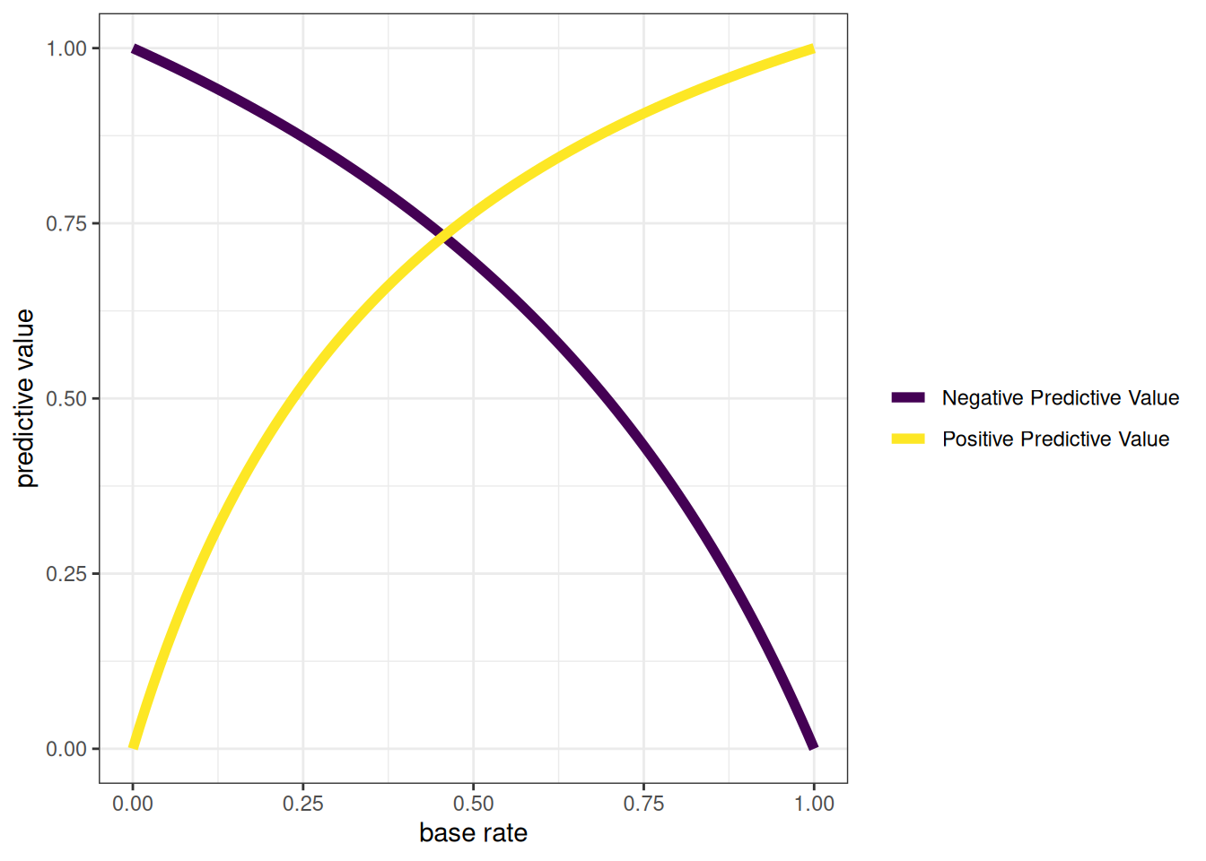
Below I compute PPV and NPV at every possible cutoff.
Code
accuracyStats$positivePredictiveValue <- positivePredictiveValue(
  TP = accuracyStats$TP,
  TN = accuracyStats$TN,
  FP = accuracyStats$FP,
  FN = accuracyStats$FN)

accuracyStats$negativePredictiveValue <- negativePredictiveValue(
  TP = accuracyStats$TP,
  TN = accuracyStats$TN,
  FP = accuracyStats$FP,
  FN = accuracyStats$FN)

ppvNPVcutoffData <- pivot_longer(
  accuracyStats,
  cols = all_of(c(
    "positivePredictiveValue","negativePredictiveValue")))
Code
ggplot(ppvNPVcutoffData, aes(x = cutoff, y = value, color = name)) +
  geom_line(linewidth = 2) +
  scale_x_continuous(name = "cutoff (liberal to conservative)", limits = c(0.05,2.09)) +
  scale_y_continuous(name = "predictive value") +
  scale_color_viridis_d(name = "", breaks = c("negativePredictiveValue","positivePredictiveValue"), labels = c("Negative Predictive Value","Positive Predictive Value")) +
  theme_bw()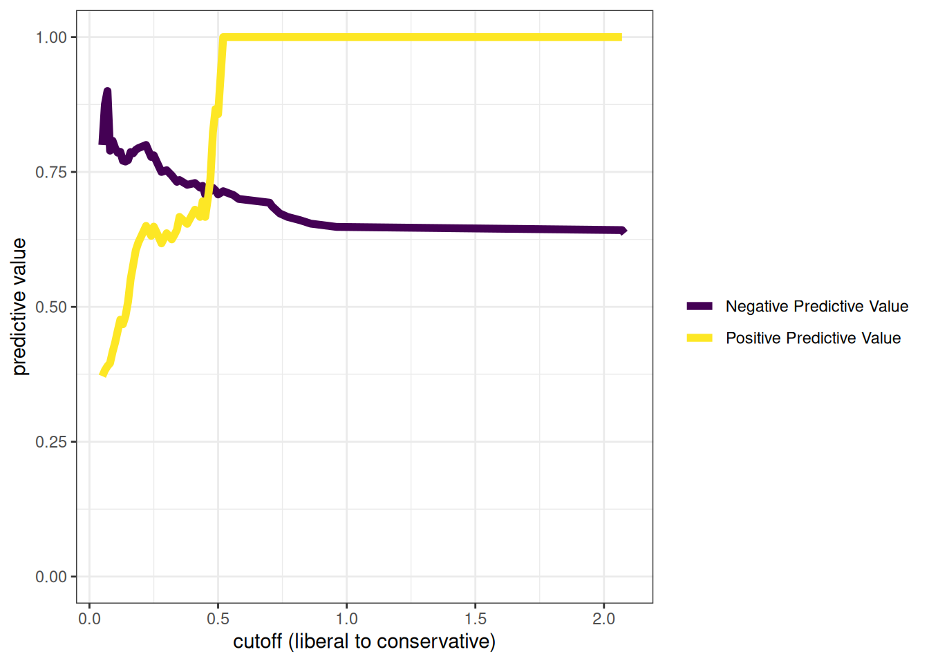
9.5.22 Negative Predictive Value (NPV)
The negative predictive value (NPV) is also called the negative predictive power (NPP). Many people confuse specificity (\(P(\text{not } R|\text{not } C)\)) with its inverse conditional probability, NPV (\(P(\text{not } C| \text{not } R)\)). NPV is the conditional probability of not having the condition given a negative test: \(P(\text{not } C| \text{not } R)\). Higher values reflect greater accuracy. The formula for calculating negative predictive value is in Equation 9.52.
NPV can be low even when specificity is high because it depends not only on specificity, but also on sensitivity and the base rate. Because NPV depends on the base rate, NPV is not an intrinsic property of a measure. The same measure will have a different NPV in different contexts with different base rates (Treat & Viken, 2023). As described in Section 9.1.2.6.1 and as depicted in Figure 9.31, as the base rate increases, NPV decreases. As the base rate decreases, NPV increases. NPV also differs as a function of the cutoff. As described in Section 9.1.2.6.1 and as depicted in Figure 9.32, as the cutoff increases (becomes more conservative), NPV decreases. As the cutoff decreases (becomes more liberal), NPV decreases.
\[ \small \begin{aligned} \text{negative predictive value (NPV)} &= P(\text{not } C|\text{not } R) \\ &= \frac{\text{TN}}{\text{TN} + \text{FN}} = \frac{\text{TN}}{N(\text{1 - SR})}\\ &= \frac{\text{specificity} \times (1-{\text{BR}})}{\text{specificity} \times (1-{\text{BR}}) + [(1 - \text{sensitivity}) \times \text{BR}]} \end{aligned} \tag{9.52}\]
9.5.23 False Discovery Rate (FDR)
Many people confuse the false positive rate (\(P(R|\text{not } C)\)) with its inverse conditional probability, the false discovery rate (\(P(\text{not } C| R)\)). The false discovery rate (FDR) is the conditional probability of not having the condition given a positive test: \(P(\text{not } C| R)\). Lower values reflect greater accuracy. The formula for calculating false discovery rate is in Equation 9.53.
\[ \begin{aligned} \text{false discovery rate (FDR)} &= P(\text{not } C|R) \\ &= \frac{\text{FP}}{\text{FP} + \text{TP}} = 1 - \text{PPV} \end{aligned} \tag{9.53}\]
9.5.24 False Omission Rate (FOR)
Many people confuse the false negative rate (\(P(\text{not } R|C)\)) with its inverse conditional probability, the false omission rate (\(P(C|\text{not } R)\)). The false omission rate (FOR) is the conditional probability of having the condition given a negative test: \(P(C|\text{not } R)\). Lower values reflect greater accuracy. The formula for calculating false omission rate is in Equation 9.54.
\[ \begin{aligned} \text{false omission rate (FOR)} &= P(C|\text{not } R) \\ &= \frac{\text{FN}}{\text{FN} + \text{TN}} = 1 - \text{NPV} \end{aligned} \tag{9.54}\]
9.5.25 Youden’s J Statistic
Youden’s J statistic is also called Youden’s Index or informedness. Youden’s J statistic is the sum of sensitivity and specificity (and subtracting one). Higher values reflect greater accuracy. The formula for calculating Youden’s J statistic is in Equation 9.55.
\[ \begin{aligned} \text{Youden's J statistic} &= \text{sensitivity} + \text{specificity} - 1 \end{aligned} \tag{9.55}\]
9.5.26 Balanced Accuracy
Balanced accuracy is the average of sensitivity and specificity. Higher values reflect greater accuracy. The formula for calculating balanced accuracy is in Equation 9.56.
\[ \begin{aligned} \text{balanced accuracy} &= \frac{\text{sensitivity} + \text{specificity}}{2} \end{aligned} \tag{9.56}\]
9.5.27 F-Score
The F-score combines precision (positive predictive value) and recall (sensitivity), where \(\beta\) indicates how many times more important sensitivity is than the positive predictive value. If sensitivity and the positive predictive value are equally important, \(\beta = 1\), and the F-score is called the \(F_1\) score. Higher values reflect greater accuracy. The formula for calculating the F-score is in Equation 9.57.
\[ \begin{aligned} F_\beta &= (1 + \beta^2) \cdot \frac{\text{positive predictive value} \cdot \text{sensitivity}}{(\beta^2 \cdot \text{positive predictive value}) + \text{sensitivity}} \\ &= \frac{(1 + \beta^2) \cdot \text{TP}}{(1 + \beta^2) \cdot \text{TP} + \beta^2 \cdot \text{FN} + \text{FP}} \end{aligned} \tag{9.57}\]
The \(F_1\) score is the harmonic mean of sensitivity and positive predictive value. The formula for calculating the \(F_1\) score is in Equation 9.58.
\[ \begin{aligned} F_1 &= \frac{2 \cdot \text{positive predictive value} \cdot \text{sensitivity}}{(\text{positive predictive value}) + \text{sensitivity}} \\ &= \frac{2 \cdot \text{TP}}{2 \cdot \text{TP} + \text{FN} + \text{FP}} \end{aligned} \tag{9.58}\]
9.5.28 Matthews Correlation Coefficient (MCC)
The Matthews correlation coefficient (MCC) is also called the phi coefficient. It is a correlation coefficient between predicted and observed values from a binary classification. Higher values reflect greater accuracy. The formula for calculating the MCC is in Equation 9.59.
\[ \begin{aligned} \text{MCC} &= \frac{\text{TP} \times \text{TN} - \text{FP} \times \text{FN}}{\sqrt{(\text{TP} + \text{FP})(\text{TP} + \text{FN})(\text{TN} + \text{FP})(\text{TN} + \text{FN})}} \end{aligned} \tag{9.59}\]
9.5.29 Diagnostic Odds Ratio
The diagnostic odds ratio is the odds of a positive test among people with the condition relative to the odds of a positive test among people without the condition. Higher values reflect greater accuracy. The formula for calculating the diagnostic odds ratio is in Equation 9.60. If the predictor is bad, the diagnostic odds ratio could be less than one, and values can go up from there. If the diagnostic odds ratio is greater than 2, we take the odds ratio seriously because we are twice as likely to predict accurately than inaccurately. However, the diagnostic odds ratio ignores/hides base rates. When interpreting the diagnostic odds ratio, it is important to keep in mind the clinical significance, because otherwise it is not very meaningful. Consider a risk factor that has a diagnostic odds ratio of 3 for tuberculosis, i.e., it puts you at 3 times as likely to develop tuberculosis. The prevalence of tuberculosis is relatively low. Assuming the prevalence of tuberculosis is less than 1/10th of 1%, your risk of developing tuberculosis is still very low even if the risk factor (with a diagnostic odds ratio of 3) is present.
\[ \begin{aligned} \text{diagnostic odds ratio} &= \frac{\text{TP} \times \text{TN}}{\text{FP} \times \text{FN}} \\ &= \frac{\text{sensitivity} \times \text{specificity}}{(1 - \text{sensitivity}) \times (1 - \text{specificity})} \\ &= \frac{\text{PPV} \times \text{NPV}}{(1 - \text{PPV}) \times (1 - \text{NPV})} \\ &= \frac{\text{LR+}}{\text{LR}-} \end{aligned} \tag{9.60}\]
9.5.30 Diagnostic Likelihood Ratio
A likelihood ratio is the ratio of two probabilities. It can be used to compare the likelihood of two possibilities. The diagnostic likelihood ratio is an index of the predictive validity of an instrument: it is the ratio of the probability that a test result is correct to the probability that the test result is incorrect. The diagnostic likelihood ratio is also called the risk ratio. There are two types of diagnostic likelihood ratios: the positive likelihood ratio and the negative likelihood ratio.
9.5.30.1 Positive Likelihood Ratio (LR+)
The positive likelihood ratio (LR+) compares the true positive rate to the false positive rate. Positive likelihood ratio values range from 1 to infinity. Higher values reflect greater accuracy, because it indicates the degree to which a true positive is more likely than a false positive. The formula for calculating the positive likelihood ratio is in Equation 9.61.
\[ \begin{aligned} \text{positive likelihood ratio (LR+)} &= \frac{\text{TPR}}{\text{FPR}} \\ &= \frac{P(R|C)}{P(R|\text{not } C)} \\ &= \frac{P(R|C)}{1 - P(\text{not } R|\text{not } C)} \\ &= \frac{\text{sensitivity}}{1 - \text{specificity}} \end{aligned} \tag{9.61}\]
9.5.30.2 Negative Likelihood Ratio (LR−)
The negative likelihood ratio (LR−) compares the false negative rate to the true negative rate. Negative likelihood ratio values range from 0 to 1. Smaller values reflect greater accuracy, because it indicates that a false negative is less likely than a true negative. The formula for calculating the negative likelihood ratio is in Equation 9.62.
\[ \begin{aligned} \text{negative likelihood ratio } (\text{LR}-) &= \frac{\text{FNR}}{\text{TNR}} \\ &= \frac{P(\text{not } R|C)}{P(\text{not } R|\text{not } C)} \\ &= \frac{1 - P(R|C)}{P(\text{not } R|\text{not } C)} \\ &= \frac{1 - \text{sensitivity}}{\text{specificity}} \end{aligned} \tag{9.62}\]
9.5.31 Posttest Odds
As presented in Equation 9.16, the posttest (or posterior) odds are equal to the pretest odds multiplied by the likelihood ratio. The posttest odds and posttest probability can be useful to calculate when the pretest probability is different from the pretest probability (or prevalence) of the classification. For instance, you might use a different pretest probability if a test result is already known and you want to know the updated posttest probability after conducting a second test. The formula for calculating posttest odds is in Equation 9.63.
\[ \begin{aligned} \text{posttest odds} &= \text{pretest odds} \times \text{likelihood ratio} \\ \end{aligned} \tag{9.63}\]
For calculating the posttest odds of a true positive compared to a false positive, we use the positive likelihood ratio, described later. We would use the negative likelihood ratio if we wanted to calculate the posttest odds of a false negative compared to a true negative.
Code
posttestOdds <- function(TP, TN, FP, FN, pretestProb = NULL, SN = NULL, SP = NULL, likelihoodRatio = NULL){
  if(!is.null(pretestProb) & !is.null(SN) & !is.null(SP)){
    pretestProbability <- pretestProb
    pretestOdds <- pretestProbability / (1 - pretestProbability)

    likelihoodRatio <- SN/(1 - SP)
  } else if(!is.null(pretestProb) & !is.null(likelihoodRatio)){
    pretestProbability <- pretestProb
    pretestOdds <- pretestProbability / (1 - pretestProbability)

    likelihoodRatio <- likelihoodRatio
  } else {
    N <- TP + TN + FP + FN
    pretestProbability <- (TP + FN)/N
    pretestOdds <- pretestProbability / (1 - pretestProbability)

    SN <- TP/(TP + FN)
    SP <- TN/(TN + FP)
    likelihoodRatio <- SN/(1 - SP)
  }

  value <- pretestOdds * likelihoodRatio

  return(value)
}[1] 1.857143Code
[1] 1.857143Code
[1] 1.8571439.5.32 Posttest Probability
The posttest probability is the probability of having the disorder given a test result. When the base rate is used as the pretest probability, the posttest probability given a positive test is equal to positive predictive value. To convert odds to a probability, divide the odds by one plus the odds, as is in Equation 9.64.
\[ \begin{aligned} \text{posttest probability} &= \frac{\text{posttest odds}}{1 + \text{posttest odds}} \end{aligned} \tag{9.64}\]
Code
posttestProbability <- function(TP, TN, FP, FN, pretestProb = NULL, SN = NULL, SP = NULL, likelihoodRatio = NULL){
  if(!is.null(pretestProb) & !is.null(SN) & !is.null(SP)){
    pretestProbability <- pretestProb
    pretestOdds <- pretestProbability / (1 - pretestProbability)

    likelihoodRatio <- SN/(1 - SP)
  } else if(!is.null(pretestProb) & !is.null(likelihoodRatio)){
    pretestProbability <- pretestProb
    pretestOdds <- pretestProbability / (1 - pretestProbability)

    likelihoodRatio <- likelihoodRatio
  } else {
    N <- TP + TN + FP + FN
    pretestProbability <- (TP + FN)/N
    pretestOdds <- pretestProbability / (1 - pretestProbability)

    SN <- TP/(TP + FN)
    SP <- TN/(TN + FP)
    likelihoodRatio <- SN/(1 - SP)
  }

  posttestOdds <- pretestOdds * likelihoodRatio
  value <- posttestOdds / (1 + posttestOdds)

  return(value)
}[1] 0.65Code
[1] 0.65Code
[1] 0.65Consider the following example: Assume the base rate of the condition is .03%. We have two tests. Test A has a sensitivity of .95 and a specificity of .80. Test B has a sensitivity of .70 and a specificity of .90. What is the probability of having the condition if a person has a positive test on Test A? Assuming the errors of the two tests are independent, what is the probability of having the condition if the person has a positive test on Test B after having a positive test on Test A?
Code
[1] 0.01409147[1] 0.09095054The probability of having the condition if a person has a positive test on Test A is \(1.4\)%. The probability of having the condition if the person has a positive test on Test B after having a positive test on Test A is \(9.1\)%.
9.5.33 Probability Nomogram
The petersenlab package (Petersen, 2025) contains the nomogrammer() function that creates a probability nomogram plot, adapted from https://github.com/achekroud/nomogrammer. In Figure 9.33, the probability nomogram is generated using the number of true positives, true negatives, false positives, and false negatives at a given cutoff.
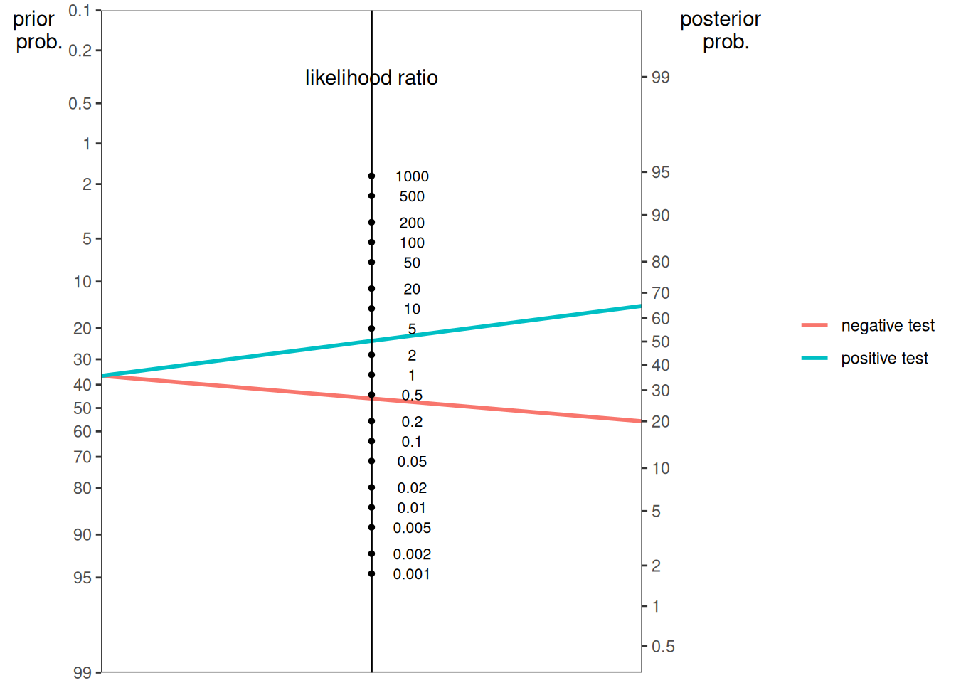
The blue line indicates the posterior probability of the condition given a positive test. The pink line indicates the posterior probability of the condition given a negative test. One can also generate the probability nomogram from the base rate and the sensitivity and specificity of the test at a given cutoff:
One can also generate the probability nomogram from the base rate, positive likelihood ratio, and negative likelihood ratio at a given cutoff:
9.5.34 \(d'\) Sensitivity from Signal Detection Theory
\(d'\) (\(d\) prime) is an index of sensitivity from signal detection theory, as described by Stanislaw & Todorov (1999). Higher values reflect greater accuracy. The formula for calculating \(d'\) is in Equation 9.65.
\[ d' = z(\text{hit rate}) - z(\text{false alarm rate}) \tag{9.65}\]
9.5.35 \(A\) (Non-Parametric) Sensitivity from Signal Detection Theory
\(A\) is a non-parametric index of sensitivity from signal detection theory, as described by Zhang & Mueller (2005). Higher values reflect greater accuracy. The formula for calculating \(A\) is in Equation 9.66.
https://sites.google.com/a/mtu.edu/whynotaprime/ (archived at https://perma.cc/W2M2-39TJ)
\[ A = \begin{cases} \frac{3}{4} + \frac{H - F}{4} - F(1 - H) & \text{if } F \leq 0.5 \leq H ; \\ \frac{3}{4} + \frac{H - F}{4} - \frac{F}{4H} & \text{if } F \leq H \leq 0.5 ;\\ \frac{3}{4} + \frac{H - F}{4} - \frac{1 - H}{4(1 - F)} & \text{if } 0.5 \leq F \leq H . \end{cases} \tag{9.66}\]
where \(H\) is the hit rate and \(F\) is the false alarm rate.
Code
aSDT <- function(TP, TN, FP, FN){
  HR <- TP/(TP + FN)
  FAR <- FP/(FP + TN)

  ifelse(FAR <= .5 & HR >= .5, value <- (3/4) + ((HR - FAR)/4) - (FAR * (1 - HR)), NA)
  ifelse(FAR <= HR & HR <= .5, value <- (3/4) + ((HR - FAR)/4) - (FAR/(4 * HR)), NA)
  ifelse(FAR >= .5 & FAR <= HR, value <- (3/4) + ((HR - FAR)/4) - ((1 - HR)/(4 * (1 - FAR))), NA)

  return(value)
}9.5.36 \(\beta\) Bias from Signal Detection Theory
\(\beta\) is an index of bias from signal detection theory, as described by Stanislaw & Todorov (1999). Smaller values reflect greater accuracy. The formula for calculating \(\beta\) is in Equation 9.67.
\[ \beta = e^{\bigg\{\frac{\big[\phi^{-1}(F)\big]^2 - \big[\phi^{-1}(H)\big]}{2}\bigg\}^2} \tag{9.67}\]
where \(H\) is the hit rate, \(F\) is the false alarm rate, and \(\phi\) (phi) is a mathematical function that converts a z score to a probability by determining the portion of the normal distribution that lies to the left of the z score.
9.5.37 \(c\) Bias from Signal Detection Theory
\(c\) is an index of bias from signal detection theory, as described by Stanislaw & Todorov (1999). Smaller values reflect greater accuracy. The formula for calculating \(c\) is in Equation 9.68.
\[ c = - \frac{\phi^{-1}(H) + \phi^{-1}(F)}{2} \tag{9.68}\]
where \(H\) is the hit rate, \(F\) is the false alarm rate, and \(\phi\) (phi) is a mathematical function that converts a z score to a probability by determining the portion of the normal distribution that lies to the left of the z score.
9.5.38 \(b\) (Non-Parametric) Bias from Signal Detection Theory
\(b\) is a non-parametric index of bias from signal detection theory, as described by Zhang & Mueller (2005). Smaller values reflect greater accuracy. The formula for calculating \(b\) is in Equation 9.69.
\[ b = \begin{cases} \frac{5 - 4H}{1 + 4F} & \text{if } F \leq 0.5 \leq H ; \\ \frac{H^2 + H}{H^2 + F} & \text{if } F \leq H \leq 0.5 ;\\ \frac{(1 - F)^2 + (1 - H)}{(1 - F)^2 + (1 - F)} & \text{if } 0.5 \leq F \leq H . \end{cases} \tag{9.69}\]
Code
bSDT <- function(TP, TN, FP, FN){
  HR <- TP/(TP + FN)
  FAR <- FP/(FP + TN)

  ifelse(FAR <= .5 & HR >= .5, value <-(5 - (4 * HR))/(1 + (4 * FAR)), NA)
  ifelse(FAR <= HR & HR <= .5, value <- (HR^2 + HR)/(HR^2 + FAR), NA)
  ifelse(FAR >= .5 & FAR <= HR, value <- ((1 - FAR)^2 + (1 - HR))/((1 - FAR)^2 + (1 - FAR)), NA)

  return(value)
}9.5.39 Mean Difference between Predicted Versus Observed Values (Miscalibration)
The mean difference between predicted values versus observed values at a given cutoff is an index of miscalibration of predictions at that cutoff. It is called “calibration-in-the-small” (as opposed to calibration-in-the-large, which spans all cutoffs). Values closer to zero reflect greater accuracy. Values above zero indicate that the predicted values are, on average, greater than the observed values. Values below zero indicate that the observed values are, on average, greater than the predicted values.
Code
miscalibration <- function(predicted, actual, cutoff, bins = 10){
  data <- data.frame(na.omit(cbind(predicted, actual)))

  calibrationTable <- mutate(
    data,
    bin = cut_number(
      predicted,
      n = 10)) %>%
    group_by(bin) %>%
    summarise(
      n = length(predicted),
      meanPredicted = mean(predicted, na.rm = TRUE),
      meanObserved = mean(actual, na.rm = TRUE),
      .groups = "drop")

  calibrationTable$cutoffMin <- as.numeric(str_replace_all(str_split(
    calibrationTable$bin,
    pattern = ",",
    simplify = TRUE)[,1],
    "[^[:alnum:]\\-\\.]", ""))
  calibrationTable$cutoffMax <- as.numeric(str_replace_all(str_split(
    calibrationTable$bin,
    pattern = ",",
    simplify = TRUE)[,2],
    "[^[:alnum:]\\-\\.]", ""))

  calibrationTable$inRange <- with(
    calibrationTable,
    cutoff >= cutoffMin & cutoff <= cutoffMax)

  if(length(which(calibrationTable$inRange == TRUE)) > 0){
    nearestCutoff <- calibrationTable$bin[min(which(
      calibrationTable$inRange == TRUE))]
    calibrationAtNearestCutoff <- calibrationTable[which(
      calibrationTable$bin == nearestCutoff),]
    calibrationAtNearestCutoff <- as.data.frame(calibrationTable[max(which(
      calibrationTable$inRange == TRUE)),])

    meanPredicted <- calibrationAtNearestCutoff[, "meanPredicted"]
    meanObserved <- calibrationAtNearestCutoff[, "meanObserved"]
    differenceBetweenPredictedAndObserved <- meanPredicted - meanObserved
  } else{
    differenceBetweenPredictedAndObserved <- NA
  }

  return(differenceBetweenPredictedAndObserved)
}9.6 Optimal Cutoff Specification
There are two ways to improve diagnostic performance (Swets et al., 2000). One way is to increase the diagnostic accuracy of the assessment. The second way is to increase the utility of the diagnostic decisions that are made, based on where we set the cutoff. The optimal cutoff depends on the differential costs of false positives versus false negatives, as applied in decision theory. When differential costs of false positives versus false negatives cannot be specified, an alternative approach to specifying the optimal cutoff is to use information theory.
9.6.1 Decision Theory
According to the decision theory approach to picking the optimal cutoff, the optimal cutoff depends on the value/importance placed on each of the four decision outcomes [(true positives, true negatives, false positives, false negatives); Treat & Viken (2023)]. Utility is the relative value placed on a specific decision-making outcome (i.e., user-perceived benefit or cost): utilities typically range between zero and one, where a value of zero represents the least desired outcome, and a value of one indicates the most desired outcome. According to the decision theory approach, the optimal cutoff is the cutoff with the highest overall utility.
9.6.1.1 Overall utility of a specific cutoff value
The overall utility of a specific cutoff value is a utilities-weighted sum of the probabilities of the four decision-making outcomes (hits, misses, correct rejections, false alarms). That is, overall utility is the sum of the product of the probability of a particular outcome (TP, TN, FP, FN; e.g., \(\text{BR} \times \text{TP rate}\)) and the utility of that outcome (e.g., how much we value TPs relative to other outcomes). Higher values reflect greater utility, so you would pick the cutoff with the highest overall utility. The formula for calculating overall utility is in Equation 9.70:
\[ \begin{aligned} U_\text{overall} = \ & (\text{BR})(\text{HR})(U_\text{H}) \\ &+ (\text{BR})(1 - \text{HR})(U_\text{M}) \\ &+ (1 - \text{BR})(\text{FAR})(U_\text{FA}) \\ &+ (1 - \text{BR})(1 - \text{FAR})(U_\text{CR}) \end{aligned} \tag{9.70}\]
where \(\text{BR} = \text{base rate}\), \(\text{HR} = \text{hit rate (true positive rate)}\), \(\text{FAR} = \text{false alarm rate (false positive rate)}\), \(U_\text{H} = \text{utility of hits (true positives)}\), \(U_\text{M} = \text{utility of misses (false negatives)}\), \(U_\text{FA} = \text{utility of false alarms (false positives)}\), \(U_\text{CR} = \text{utility of correct rejections (true negatives)}\).
Code
[1] 0.65Code
[1] 0.7454545Code
[1] 0.71818189.6.1.2 Utility ratio
The utility ratio is the user-perceived relative importance of decisions about negative versus positive cases. If the utility ratio value is one, it indicates that identifying negative cases and positive cases is equally important. Values above one indicate greater relative importance of identifying negative cases than positive cases. Values below one indicate greater relative importance of identifying positive cases than negative cases. Values of one indicate that you are maximizing percent accuracy. The formula for calculating the utility ratio is in Equation 9.71:
\[ \text{Utility Ratio} = \frac{U_\text{CR} - U_\text{FA}}{U_\text{H} - U_\text{M}} \tag{9.71}\]
where \(U_\text{H} = \text{utility of hits (true positives)}\), \(U_\text{M} = \text{utility of misses (false negatives)}\), \(U_\text{FA} = \text{utility of false alarms (false positives)}\), \(U_\text{CR} = \text{utility of correct rejections (true negatives)}\).
[1] 0.5[1] 1[1] 2Decision theory has key advantages, because it identifies the cutoff that would help you best achieve the goals/purpose of the assessment. However, it can be challenging to specify the relative costs of errors. If you cannot decide values for outcomes (relative importance between FP and FN), you can use information theory to identify the optimal cutoff.
9.6.2 Information Theory
When the user does not differentially weigh the value/importance of the four decision-making outcomes (hits, misses, correct rejections, false alarms), the information theory approach can be useful for specifying the optimal cutoff. According to the information theory approach, the optimal cutoff is the cutoff that provides the greatest information gain (Treat & Viken, 2023).
9.6.2.1 Information Gain
Information gain (\(I_\text{gain}\)) is the reduction of uncertainty about the true classification of a case that results from administering an assessment or prediction measure (Treat & Viken, 2023). Greater values reflect greater reduction of uncertainty, so the optimal cutoff can be specified as the cutoff with the highest information gain.
9.6.2.1.1 Formula from Treat & Viken (2023)
The formula from Treat & Viken (2023) for calculating information gain is in Equation 9.72:
\[ \begin{aligned} I_\text{gain} = \ & (\text{BR})(\text{HR})\bigg[\log_2\bigg(\frac{\text{HR}}{G}\bigg)\bigg] \\ &+ (\text{BR})(1 - \text{HR})\bigg[\log_2\bigg(\frac{1 - \text{HR}}{1 - G}\bigg)\bigg] \\ &+ (1 - \text{BR})(\text{FAR})\bigg[\log_2\bigg(\frac{\text{FAR}}{G}\bigg)\bigg] \\ &+ (1 - \text{BR})(1 - \text{FAR})\bigg[\log_2\bigg(\frac{1 - \text{FAR}}{1 - G}\bigg)\bigg] \end{aligned} \tag{9.72}\]
where \(\text{BR} =\) base rate, \(\text{HR} =\) hit rate (true positive rate), \(\text{FAR} =\) false alarm rate (false positive rate), \(G =\) selection ratio \(= \text{BR} (\text{HR}) + (1 - \text{BR}) (\text{FAR})\), as reported in Somoza et al. (1989) (see below).
9.6.2.1.2 Alternative formula from Metz et al. (1973)
The alternative formula from Metz et al. (1973) for calculating information gain is in Equation 9.73:
\[ \begin{aligned} I_\text{gain} = \ & p(S|s) \cdot p(s) \cdot log_2\Bigg\{\frac{p(S|s)}{p(S|s) \cdot p(s) + p(S|n)[1 - p(s)]}\Bigg\} \\ &+ p(S|n)[1 - p(s)] \times log_2\Bigg\{\frac{p(S|n)}{p(S|s) \cdot p(s) + p(S|n)[1 - p(s)]}\Bigg\} \\ &+ [1 - p(S|s)] \cdot p(s) \times log_2\Bigg\{\frac{1 - p(S|s)}{1 - p(S|s) \cdot p(s) - p(S|n)[1 - p(s)]}\Bigg\} \\ &+ [1 - p(S|n)][1 - p(s)] \times log_2\Bigg\{\frac{1 - p(S|n)}{1 - p(S|s) \cdot p(s) - p(S|n)[1 - p(s)]}\Bigg\} \end{aligned} \tag{9.73}\]
where \(p(S|s) =\) sensitivity (hit rate or true positive rate); i.e., the conditional probability of deciding a signal is present (\(S\)) when the signal is in fact present(\(s\)), \(p(S|n) =\) false positive rate (false alarm rate); i.e., the conditional probability of deciding a signal is present (\(S\)) when the signal is in fact absent (\(n\)), \(p(s) =\) base rate, i.e., the probability that the signal is in fact present (\(s\)).
Code
9.6.2.1.3 Alternative formula from Somoza et al. (1989)
The alternative formula from Somoza et al. (1989) for calculating information gain is in Equation 9.74:
\[ \begin{aligned} I_\text{gain} = \ & [(\text{TPR})(\text{Pr})] \times \log_2(\text{TPR}/G) \\ &+ [(\text{FPR})(1 - \text{Pr})] \times \log_2(\text{FPR}/G) \\ &+ [(1 - \text{TPR})(\text{Pr})] \times \log_2\bigg(\frac{1 - \text{TPR}}{1 - G}\bigg) \\ &+ [(1 - \text{FPR})(1 - \text{Pr})] \times \log_2\bigg(\frac{1 - \text{FPR}}{1 - G}\bigg) \end{aligned} \tag{9.74}\]
where \(\text{TP} =\) true positive rate (hit rate), \(\text{Pr} =\) prevalence (base rate), \(\text{FP} =\) false positive rate (false alarm rate), \(G = \text{Pr} (\text{TP}) + (1 - \text{Pr}) (\text{FP}) =\) selection ratio
9.6.2.1.4 Examples
Case A from Exhibit 38.2 (Treat & Viken, 2023):
Case B from Exhibit 38.2 (Treat & Viken, 2023):
Case C from Exhibit 38.2 (Treat & Viken, 2023):
Case B from Exhibit 38.3 (Treat & Viken, 2023):
9.6.2.1.5 Effect of Base Rate
Information gain depends on the base rate (Treat & Viken, 2023), as depicted in Figure 9.34. The maximum reduction of uncertainty (i.e., greatest information) occurs when the base rate is 0.5. A base rate tells us little a priori about the condition if the probability of the condition is 50/50, so the measure can provide more benefit. If the base rate is 0.3 or 0.7, we can do better than going with the base rate. If the base rate is 0.9 or 0.1, it is difficult for our measure to do better than going with the base rate. If the base rate is 0.05 of 0.95 (or more extreme), it is likely that our measure will do almost nothing in terms of information gain.
Code
possibleCutoffs <- unique(na.omit(mydataSDT$testScore))
possibleCutoffs <- possibleCutoffs[order(possibleCutoffs)]
possibleCutoffs <- c(possibleCutoffs, max(possibleCutoffs, na.rm = TRUE) + 0.01)
baseRates <- c(.05, .1, .3, .5, .7, .9, .95)
possibleCutoffsBaseRates <- expand_grid(baseRate = baseRates, cutoff = possibleCutoffs)
informationGainVars <- c("cutoff","TP","TN","FP","FN")
informationGainStats <- data.frame(matrix(nrow = length(possibleCutoffs), ncol = length(informationGainVars)))
names(informationGainStats) <- informationGainVars
for(i in 1:length(possibleCutoffs)){
cutoff <- possibleCutoffs[i]
mydataSDT$diagnosis <- NA
mydataSDT$diagnosis[mydataSDT$testScore < cutoff] <- 0
mydataSDT$diagnosis[mydataSDT$testScore >= cutoff] <- 1
informationGainStats[i, "cutoff"] <- cutoff
informationGainStats[i, "TP"] <- length(which(mydataSDT$diagnosis == 1 & mydataSDT$disorder == 1))
informationGainStats[i, "TN"] <- length(which(mydataSDT$diagnosis == 0 & mydataSDT$disorder == 0))
informationGainStats[i, "FP"] <- length(which(mydataSDT$diagnosis == 1 & mydataSDT$disorder == 0))
informationGainStats[i, "FN"] <- length(which(mydataSDT$diagnosis == 0 & mydataSDT$disorder == 1))
}
informationGainStats <- full_join(possibleCutoffsBaseRates, informationGainStats, by = "cutoff")
informationGainStats$TPrate <- sensitivity(TP = informationGainStats$TP, TN = informationGainStats$TN, FP = informationGainStats$FP, FN = informationGainStats$FN)
informationGainStats$FPrate <- falsePositiveRate(TP = informationGainStats$TP, TN = informationGainStats$TN, FP = informationGainStats$FP, FN = informationGainStats$FN)
informationGainStats$informationGain <- Igain(BR = informationGainStats$baseRate, HR = informationGainStats$TPrate, FAR = informationGainStats$FPrate)
informationGainStats <- na.omit(informationGainStats)
ggplot(
data = informationGainStats,
aes(
x = cutoff,
y = informationGain,
group = as.factor(baseRate),
color = as.factor(baseRate))) +
geom_line(linewidth = 2) +
scale_x_continuous(name = "Cutoff") +
scale_y_continuous(name = "Information Gain") +
scale_color_viridis(
name = "Base Rate",
discrete = TRUE,
option = "H") +
geom_label_repel(
data = informationGainStats %>%
filter(cutoff == 0.5),
aes(label = paste("BR = ", baseRate, sep = "")),
nudge_x = 0.10,
na.rm = TRUE) +
theme_bw() +
theme(legend.position = "none")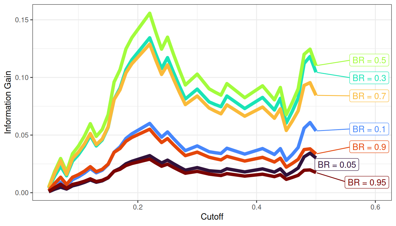
9.7 Accuracy at Every Possible Cutoff
9.7.1 Specify utility of each outcome
9.7.2 Calculate Accuracy
Code
possibleCutoffs <- unique(na.omit(mydataSDT$testScore))
possibleCutoffs <- possibleCutoffs[order(possibleCutoffs)]
possibleCutoffs <- c(
possibleCutoffs, max(possibleCutoffs, na.rm = TRUE) + 0.01)
accuracyVariables <- c(
"cutoff", "TP", "TN", "FP", "FN", "differenceBetweenPredictedAndObserved")
accuracyStats <- data.frame(
matrix(
nrow = length(possibleCutoffs),
ncol = length(accuracyVariables)))
names(accuracyStats) <- accuracyVariables
for(i in 1:length(possibleCutoffs)){
cutoff <- possibleCutoffs[i]
mydataSDT$diagnosis <- NA
mydataSDT$diagnosis[mydataSDT$testScore < cutoff] <- 0
mydataSDT$diagnosis[mydataSDT$testScore >= cutoff] <- 1
accuracyStats[i, "cutoff"] <- cutoff
accuracyStats[i, "TP"] <- length(which(
mydataSDT$diagnosis == 1 & mydataSDT$disorder == 1))
accuracyStats[i, "TN"] <- length(which(
mydataSDT$diagnosis == 0 & mydataSDT$disorder == 0))
accuracyStats[i, "FP"] <- length(which(
mydataSDT$diagnosis == 1 & mydataSDT$disorder == 0))
accuracyStats[i, "FN"] <- length(which(
mydataSDT$diagnosis == 0 & mydataSDT$disorder == 1))
accuracyStats[i, "differenceBetweenPredictedAndObserved"] <-
miscalibration(
predicted = mydataSDT$testScore,
actual = mydataSDT$disorder,
cutoff = cutoff)
}
accuracyStats$N <- sampleSize(
TP = accuracyStats$TP,
TN = accuracyStats$TN,
FP = accuracyStats$FP,
FN = accuracyStats$FN)
accuracyStats$selectionRatio <- selectionRatio(
TP = accuracyStats$TP,
TN = accuracyStats$TN,
FP = accuracyStats$FP,
FN = accuracyStats$FN)
accuracyStats$baseRate <- baseRate(
TP = accuracyStats$TP,
TN = accuracyStats$TN,
FP = accuracyStats$FP,
FN = accuracyStats$FN)
accuracyStats$percentAccuracy <- percentAccuracy(
TP = accuracyStats$TP,
TN = accuracyStats$TN,
FP = accuracyStats$FP,
FN = accuracyStats$FN)
accuracyStats$percentAccuracyByChance <- percentAccuracyByChance(
TP = accuracyStats$TP,
TN = accuracyStats$TN,
FP = accuracyStats$FP,
FN = accuracyStats$FN)
accuracyStats$relativeImprovementOverChance <- relativeImprovementOverChance(
TP = accuracyStats$TP,
TN = accuracyStats$TN,
FP = accuracyStats$FP,
FN = accuracyStats$FN)
accuracyStats$relativeImprovementOverPredictingFromBaseRate <-
relativeImprovementOverPredictingFromBaseRate(
TP = accuracyStats$TP,
TN = accuracyStats$TN,
FP = accuracyStats$FP,
FN = accuracyStats$FN)
accuracyStats$sensitivity <- accuracyStats$TPrate <- sensitivity(
TP = accuracyStats$TP,
TN = accuracyStats$TN,
FP = accuracyStats$FP,
FN = accuracyStats$FN)
accuracyStats$specificity <- accuracyStats$TNrate <- specificity(
TP = accuracyStats$TP,
TN = accuracyStats$TN,
FP = accuracyStats$FP,
FN = accuracyStats$FN)
accuracyStats$FNrate <- falseNegativeRate(
TP = accuracyStats$TP,
TN = accuracyStats$TN,
FP = accuracyStats$FP,
FN = accuracyStats$FN)
accuracyStats$FPrate <- falsePositiveRate(
TP = accuracyStats$TP,
TN = accuracyStats$TN,
FP = accuracyStats$FP,
FN = accuracyStats$FN)
accuracyStats$youdenJ <- youdenJ(
TP = accuracyStats$TP,
TN = accuracyStats$TN,
FP = accuracyStats$FP,
FN = accuracyStats$FN)
accuracyStats$positivePredictiveValue <- positivePredictiveValue(
TP = accuracyStats$TP,
TN = accuracyStats$TN,
FP = accuracyStats$FP,
FN = accuracyStats$FN)
accuracyStats$negativePredictiveValue <- negativePredictiveValue(
TP = accuracyStats$TP,
TN = accuracyStats$TN,
FP = accuracyStats$FP,
FN = accuracyStats$FN)
accuracyStats$falseDiscoveryRate <- falseDiscoveryRate(
TP = accuracyStats$TP,
TN = accuracyStats$TN,
FP = accuracyStats$FP,
FN = accuracyStats$FN)
accuracyStats$falseOmissionRate <- falseOmissionRate(
TP = accuracyStats$TP,
TN = accuracyStats$TN,
FP = accuracyStats$FP,
FN = accuracyStats$FN)
accuracyStats$balancedAccuracy <- balancedAccuracy(
TP = accuracyStats$TP,
TN = accuracyStats$TN,
FP = accuracyStats$FP,
FN = accuracyStats$FN)
accuracyStats$f1Score <- fScore(
TP = accuracyStats$TP,
TN = accuracyStats$TN,
FP = accuracyStats$FP,
FN = accuracyStats$FN)
accuracyStats$mcc <- mcc(
TP = accuracyStats$TP,
TN = accuracyStats$TN,
FP = accuracyStats$FP,
FN = accuracyStats$FN)
accuracyStats$diagnosticOddsRatio <- diagnosticOddsRatio(
TP = accuracyStats$TP,
TN = accuracyStats$TN,
FP = accuracyStats$FP,
FN = accuracyStats$FN)
accuracyStats$positiveLikelihoodRatio <- positiveLikelihoodRatio(
TP = accuracyStats$TP,
TN = accuracyStats$TN,
FP = accuracyStats$FP,
FN = accuracyStats$FN)
accuracyStats$negativeLikelihoodRatio <- negativeLikelihoodRatio(
TP = accuracyStats$TP,
TN = accuracyStats$TN,
FP = accuracyStats$FP,
FN = accuracyStats$FN)
accuracyStats$dPrimeSDT <- dPrimeSDT(
TP = accuracyStats$TP,
TN = accuracyStats$TN,
FP = accuracyStats$FP,
FN = accuracyStats$FN)
accuracyStats$betaSDT <- betaSDT(
TP = accuracyStats$TP,
TN = accuracyStats$TN,
FP = accuracyStats$FP,
FN = accuracyStats$FN)
accuracyStats$cSDT <- cSDT(
TP = accuracyStats$TP,
TN = accuracyStats$TN,
FP = accuracyStats$FP,
FN = accuracyStats$FN)
accuracyStats$ASDT <- aSDT(
TP = accuracyStats$TP,
TN = accuracyStats$TN,
FP = accuracyStats$FP,
FN = accuracyStats$FN)
accuracyStats$bSDT <- bSDT(
TP = accuracyStats$TP,
TN = accuracyStats$TN,
FP = accuracyStats$FP,
FN = accuracyStats$FN)
accuracyStats$overallUtility <- Uoverall(
BR = accuracyStats$baseRate,
HR = accuracyStats$TPrate,
FAR = accuracyStats$FPrate,
UH = utilityHits,
UM = utilityMisses,
UCR = utilityCorrectRejections,
UFA = utilityFalseAlarms)
accuracyStats$utilityRatio <- utilityRatio(
UH = utilityHits,
UM = utilityMisses,
UCR = utilityCorrectRejections,
UFA = utilityFalseAlarms)
accuracyStats$informationGain <- Igain(
BR = accuracyStats$baseRate,
HR = accuracyStats$TPrate,
FAR = accuracyStats$FPrate)
#Replace NaN and INF values with NA
is.nan.data.frame <- function(x)
do.call(cbind, lapply(x, is.nan))
accuracyStats[is.nan.data.frame(accuracyStats)] <- NA
accuracyStats <- do.call(
data.frame,
lapply(
accuracyStats,
function(x) replace(x, is.infinite(x), NA)))9.7.3 All Accuracy Statistics
The petersenlab package (Petersen, 2025) contains an R function that estimates the prediction accuracy at every possible cutoff.
Code
9.7.4 Youden’s J Statistic
9.7.4.1 Threshold
Threshold at maximum combination of sensitivity and specificity:
\(\text{max}(\text{sensitivity} + \text{specificity})\)
9.7.4.2 Accuracy statistics at cutoff of Youden’s J Statistic
9.7.5 Closest to the Top Left of the ROC Curve
9.7.5.1 Threshold
Threshold where the ROC plot is closest to the Top Left:
9.7.5.2 Accuracy stats at cutoff where the ROC plot is closest to the Top Left
9.7.6 Cutoff that optimizes each of the following criteria:
The petersenlab package (Petersen, 2025) contains an R function that identifies the cutoff that optimizes each of various accuracy estimates.
Code
[[1]]
percentAccuracyCutoff percentAccuracyOptimal
1 0.22 74.54545
2 0.52 74.54545
[[2]]
percentAccuracyByChanceCutoff percentAccuracyByChanceOptimal
1 2.08 63.63636
[[3]]
RIOCCutoff RIOCOptimal
1 0.07 0.725
[[4]]
relativeImprovementOverPredictingFromBaseRateCutoff
1 0.22
2 0.52
relativeImprovementOverPredictingFromBaseRateOptimal
1 0.15
2 0.15
[[5]]
PPVCutoff PPVOptimal
1 0.52 1
2 0.56 1
3 0.58 1
4 0.70 1
5 0.71 1
6 0.74 1
7 0.77 1
8 0.82 1
9 0.86 1
10 0.96 1
11 2.07 1
[[6]]
NPVCutoff NPVOptimal
1 0.07 0.9
[[7]]
youdenJCutoff youdenJOptimal
1 0.22 0.45
[[8]]
balancedAccuracyCutoff balancedAccuracyOptimal
1 0.22 0.725
[[9]]
f1ScoreCutoff f1ScoreOptimal
1 0.22 0.65
[[10]]
mccCutoff mccOptimal
1 0.52 0.46291
[[11]]
diagnosticOddsRatioCutoff diagnosticOddsRatioOptimal
1 0.49 16.37037
[[12]]
positiveLikelihoodRatioCutoff positiveLikelihoodRatioOptimal
1 0.49 11.375
[[13]]
negativeLikelihoodRatioCutoff negativeLikelihoodRatioOptimal
1 0.07 0.1944444
[[14]]
dPrimeSDTCutoff dPrimeSDTOptimal
1 0.49 1.448454
[[15]]
betaSDTCutoff betaSDTOptimal
1 0.07 0.2784011
[[16]]
cSDTCutoff cSDTOptimal
1 0.16 0.01498818
[[17]]
aSDTCutoff aSDTOptimal
1 0.52 0.825
[[18]]
bSDTCutoff bSDTOptimal
1 0.07 0.2862166
[[19]]
differenceBetweenPredictedAndObservedCutoff
1 0.14
2 0.15
3 0.16
differenceBetweenPredictedAndObservedOptimal
1 0.058
2 0.058
3 0.058
[[20]]
informationGainCutoff informationGainOptimal
1 0.22 0.1465904
[[21]]
overallUtilityCutoff overallUtilityOptimal
1 0.22 0.659.7.6.1 Percent Accuracy
9.7.6.2 Percent Accuracy by Chance
9.7.6.3 Relative Improvement Over Chance (ROIC)
9.7.6.4 Relative Improvement Over Predicting from the Base Rate
9.7.6.5 Sensitivity
9.7.6.6 Specificity
9.7.6.7 Positive Predictive Value
9.7.6.8 Negative Predictive Value
9.7.6.9 Youden’s J Statistic
9.7.6.10 Balanced Accuracy
9.7.6.11 F1 Score
9.7.6.12 Matthews Correlation Coefficient
9.7.6.13 Diagnostic Odds Ratio
9.7.6.14 Positive Likelihood Ratio
9.7.6.15 Negative Likelihood Ratio
9.7.6.16 \(d'\) Sensitivity
9.7.6.17 \(A\) (Non-Parametric) Sensitivity
9.7.6.18 \(\beta\) Bias
9.7.6.19 \(c\) Bias
9.7.6.20 \(b\) (Non-Parametric) Bias
9.7.6.21 Mean difference between predicted and observed values (Miscalibration)
9.7.6.22 Overall Utility
9.7.6.23 Information Gain
9.8 Regression for Prediction of Continuous Outcomes
When predicting a continuous outcome, regression is particularly relevant (or multiple regression, when dealing with multiple predictors). Regression takes the general form in Equation 9.75:
\[ y = b_0 + b_1 \cdot x_1 + e \tag{9.75}\]
where \(y\) is the outcome, \(b_0\) is the intercept, \(b_1\) is the slope of the association between the predictor (\(x_1\)) and outcome, and \(e\) is the error term.
If the predictors reflect what causes the outcome, then the error term reflects what cannot be accounted for by the predictors. It has been argued that human freedom resides in the error term (Kenny, 1979).
9.9 Pseudo-Prediction
Consider the following example where you have one predictor and one outcome, as shown in Table 9.2.
| y | x1 |
|---|---|
| 7 | 1 |
| 13 | 2 |
| 29 | 7 |
| 10 | 2 |
Using the data, the best fitting regression model is: \(y = 3.98 + 3.59 \cdot x_1\). In this example, the \(R^2\) is \(0.98\). The equation is not a perfect prediction, but with a single predictor, it captures the majority of the variance in the outcome.
Now consider the following example where you add a second predictor to the data above, as shown in Table 9.3.
| y | x1 | x2 |
|---|---|---|
| 7 | 1 | 3 |
| 13 | 2 | 5 |
| 29 | 7 | 1 |
| 10 | 2 | 2 |
With the second predictor, the best fitting regression model is: \(y = 0.00 + 4.00 \cdot x_1 + 1.00 \cdot x_2\). In this example, the \(R^2\) is \(1.00\). The equation with the second predictor provides a perfect prediction of the outcome.
Providing perfect prediction with the right set of predictors is the dream of multiple regression. So, in psychology, we often add predictors to incrementally improve prediction. Knowing how much variance would be accounted for by random chance follows Equation 9.76:
\[ E(R^2) = \frac{K}{n-1} \tag{9.76}\]
where \(E(R^2)\) is the expected value of \(R^2\) (the proportion of variance explained), \(K\) is the number of predictors, and \(n\) is the sample size. The formula demonstrates that the more predictors in the regression model, the more variance will be accounted for by chance. With many predictors and a small sample, you can account for a large share of the variance merely by chance—this would be an example of pseudo-prediction.
As an example, consider that we have 13 predictors to predict behavior problems for 43 children. Assume that, with 13 predictors, we explain 38% of the variance (\(R^2 = .38; r = .62\)). Explaining more than 20–30% of the variance can be a big deal in psychology. We explained a lot of the variance in the outcome, but it is important to consider how much variance could have been explained by random chance: \(E(R^2) = \frac{K}{n-1} = \frac{13}{43 - 1} = .31\). We expect to explain 31% of the variance, by chance, in the outcome. So, 82% of the variance explained was likely spurious. As the sample size increases, the spuriousness decreases. Adjusted \(R^2\) accounts for the number of predictors in the model, based on how much would be expected to be accounted for by chance. But adjusted \(R^2\) also has its problems.
9.9.1 Multicollinearity
Multicollinearity occurs when two or more predictors in a regression model are highly correlated. The problem is that it makes it challenging to estimate the regression coefficients accurately.
Multicollinearity in multiple regression is depicted conceptually in Figure 9.35.
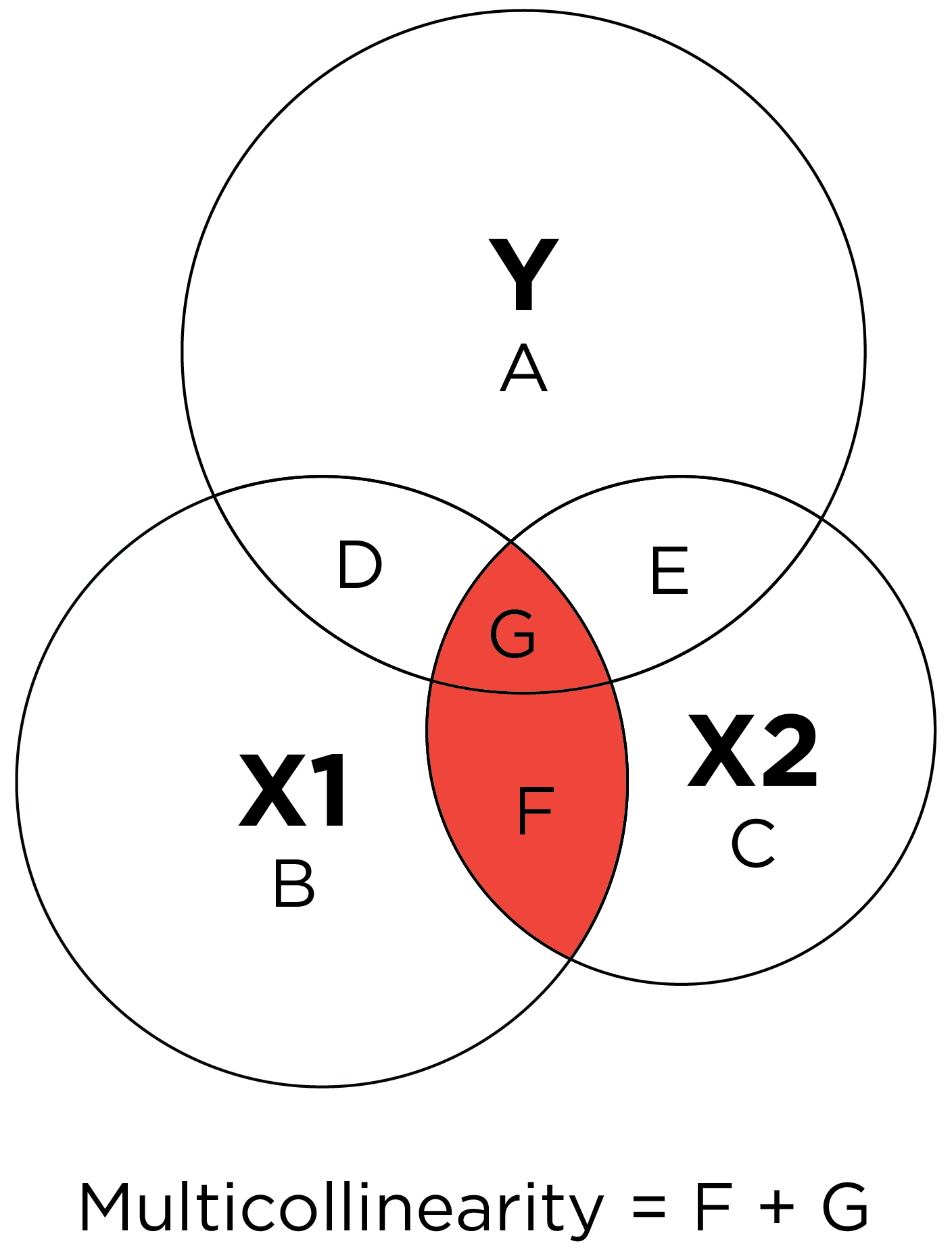
Consider the following example where you have two predictors and one outcome, as shown in Table 9.4.
| y | x1 | x2 |
|---|---|---|
| 9 | 2.0 | 4 |
| 11 | 3.0 | 6 |
| 17 | 4.0 | 8 |
| 3 | 1.0 | 2 |
| 21 | 5.0 | 10 |
| 13 | 3.5 | 7 |
The second measure is not very good—it is exactly twice the value of the first measure. This means that there are different prediction equation possibilities that are equally good—see Equation 9.77:
\[ \begin{aligned} 2x_2 &= y \\ 0x_1 + 2x_2 &= y \\ 4x_1 &= y \\ 4x_1 + 0x_2 &= y \\ 2x_1 + 1x_2 &= y \\ 5x_1 - 0.5x_2 &= y \\ ... &= y \end{aligned} \tag{9.77}\]
Then, what are the regression coefficients? We do not know, and we could come up with arbitrary estimates with an enormous standard error around each estimate. Any predictors that have a correlation above ~ \(r = .30\) with each other could have an impact on the confidence interval of the regression coefficient. As the correlations among the predictors increase, the chance of getting an arbitrary answer increases, sometimes called “bouncing betas.” So, it is important to examine a correlation matrix of the predictors before putting them in the same regression model. You can also examine indices such as variance inflation factor (VIF).
Generalized VIF (GVIF) values are estimated below using the car package (Fox et al., 2022).
Code
GVIF Df GVIF^(1/(2*Df))
ndka 6.300087 1 2.509997
gender 1.149601 1 1.072194
age 1.127608 1 1.061889
wfns 1.207583 4 1.023858
collinearPredictor 6.405020 1 2.530814To address multicollinearity, you can drop a redundant predictor or you can also use principal component analysis or factor analysis of the predictors to reduce the predictors down to a smaller number of meaningful predictors. For a meaningful answer in a regression framework that is precise and confident, you need a low level of intercorrelation among predictors, unless you have a very large sample size.
However, multicollinearity does not bias parameter estimates (i.e., multicollinearity does not lead to mean error). Instead, multicollinearity increases the uncertainty (i.e., standard errors) around the parameter estimates (archived at https://perma.cc/DJ7L-TCUK), which makes it more challenging to detect an effect as statistically significant. Some forms of multicollinearity are ignorable (archived at https://perma.cc/2JV5-2QEZ), including when the multicollinearity is among (a) the control variables rather than the variables of interest, (b) the powers (e.g., quadratic term) or products (e.g., interaction term) of other variables, or (c) dummy-coded categories. Ultimately, it is important to examine the question of interest, even if that means inclusion of predictors that are inter-correlated in a regression model (archived at https://perma.cc/DJ7L-TCUK). However, it would not make sense to include two predictors that are perfectly correlated, because they are redundant.
9.10 Ways to Improve Prediction Accuracy
On the whole, experts’ predictions are inaccurate. Experts’ predictions from many different domains tend to be inaccurate, including political scientists (Tetlock, 2017), physicians (Koehler et al., 2002), clinical psychologists (Oskamp, 1965), stock market traders and corporate financial officers (Skala, 2008), seismologists’ predictions of earthquakes (Hough, 2016), economists’ predictions about the economy (Makridakis et al., 2009), lawyers (Koehler et al., 2002), and business managers (Russo & Schoemaker, 1992). The most common pattern of experts’ predictions is that they show overextremity, that is, their predictions have probability judgments that tend to be too extreme, as described in Section 9.4.3. Overextremity of experts’ predictions likely reflects over-confidence. The degree of confidence of a person’s predictions is often not a good indicator of the accuracy of their predictions (and confidence and prediction accuracy are sometimes inversely associated; Silver, 2012). Cognitive biases including the anchoring bias (Tversky & Kahneman, 1974), the confirmation bias (Hoch, 1985; Koriat et al., 1980), and base rate neglect (Eddy, 1982; Koehler et al., 2002) could contribute to over-confidence of predictions. Poorly calibrated predictions are especially likely when the base rate is very low (e.g., suicide), as is often the case in clinical psychology, or when the base rate is very high (Koehler et al., 2002).
Nevertheless, there are some domains that have shown greater predictive accuracy, from which we may learn what practices may lead to greater accuracy. For instance, experts have shown stronger predictive accuracy in weather forecasting (Murphy & Winkler, 1984), horse race betting (Johnson & Bruce, 2001), and playing the card game of bridge (Keren, 1987), but see Koehler et al. (2002) for exceptions.
Here are some potential ways to improve the accuracy (and honesty) of predictions and judgments:
- Provide appropriate anchoring of your predictions to the base rate of the phenomenon you are predicting. To the extent that the base rate of the event you are predicting is low, more extreme evidence should be necessary to consistently and accurately predict that the event will occur. Applying Bayes’ theorem and Bayesian approaches can help you appropriately weigh base rate and evidence.
- Include multiple predictors, ideally from different measures and measurement methods. Include the predictors with the strongest validity based on theory of the causal process and based on criterion-related validity.
- When possible, aggregate multiple perspectives of predictions, especially predictions made independently (from different people/methods/etc.). The “wisdom of the crowd” is often more accurate than individuals’ predictions, including predictions by so-called “experts” (Silver, 2012).
- Instead of aggregating scores from multi-item scales, another option is to “unamalgamate” the predictors, that is, to use each item in the scale as a separate predictor, to maximize predictive power (Trafimow et al., 2025).
- A goal of prediction is to capture as much signal as possible and as little noise (error) as possible (Silver, 2012). Parsimony (i.e., not having too many predictors) can help reduce the amount of error variance captured by the prediction model. However, to accurately model complex systems like human behavior, the brain, etc., complex models may be necessary. Nevertheless, strong theory of the causal processes and dynamics may be necessary to develop accurate complex models.
- Although incorporating theory can be helpful, provide more weight to empiricism than to theory, until our theories and measures are stronger. Ideally, we would use theory to design a model that mirrors the causal system, with accurate measures of each process in the system, so we could make accurate predictions. However, as described in Section 5.3.1.3.3, our psychological theories of the causal processes that influence outcomes are not yet very strong. Until we have stronger theories that specify the causal process for a given outcome, and until we have accurate measures of those causal processes, actuarial approaches are likely to be most accurate, as discussed in Chapter 10. At the same time, keep in mind that measures in psychology, and their resulting data, are often noisy. As a result, theoretically (conceptually) informed empirical approaches may lead to more accuracy than empiricism alone.
- Use an empirically validated and cross-validated statistical algorithm to combine information from the predictors in a formalized way. Give each predictor appropriate weight in the statistical algorithm, according to its strength of association with the outcome. Use measures with strong reliability and validity for assessing these processes to be used in the algorithm. Cross-validation will help reduce the likelihood that your model is fitting to noise and will maximize the likelihood that the model predicts accurately when applied to new data (i.e., the model’s predictions accurately generalize), as described in Section 10.4.
- When presenting your predictions, acknowledge what you do not know.
- Express your predictions in terms of probabilistic estimates and present the uncertainty in your predictions with confidence intervals (even though bolder, more extreme predictions tend to receive stronger television ratings; Silver, 2012).
- Qualify your predictions by identifying and noting counter-examples that would not be well fit by your prediction model, such as extreme cases, edge cases, and “broken leg” (Meehl, 1957) cases.
- Provide clear, consistent, and timely feedback on the outcomes of the predictions to the people making the predictions (Bolger & Önkal-Atay, 2004).
- Be self-critical about your predictions. Update your judgments based on their accuracy, rather than trying to confirm your beliefs (Atanasov et al., 2020).
- In addition to considering the accuracy of the prediction, consider the quality of the prediction process, especially when random chance is involved to a degree (such as in poker) (Silver, 2012).
- Work to identify and mitigate potential blindspots; be aware of cognitive biases, such as confirmation bias and base rate neglect.
- Evaluate for the possibility of bias in the predictions or in the tests from which the predictions are derived. Correct for any test bias.
9.11 Conclusion
Human behavior is challenging to predict. People commonly make cognitive pseudo-prediction errors, such as the confusion of inverse probabilities. People also tend to ignore base rates when making predictions. When the base rate of a behavior is very low or very high, you can be highly accurate in predicting the behavior by predicting from the base rate. Thus, you cannot judge how accurate your prediction is until you know how accurate your predictions would be by random chance. Moreover, maximizing percent accuracy may not be the ultimate goal because different errors have different costs. Though there are many types of accuracy, there are two broad types: discrimination and calibration—and they are orthogonal. Discrimination accuracy is frequently evaluated with the area under the receiver operating characteristic curve, or with sensitivity and specificity, or standardized regression coefficients. Calibration accuracy is frequently evaluated graphically and with various indices. Sensitivity and specificity depend on the cutoff. Therefore, the optimal cutoff depends on the purposes of the assessment and how much one weights the various costs of the different types of errors: false negatives and false positives. It is important to evaluate both discrimination and calibration when evaluating prediction accuracy.
9.12 Suggested Readings
Steyerberg et al. (2010); Meehl & Rosen (1955); Treat & Viken (2023); Wiggins (1973)
9.13 Exercises
9.13.1 Questions
Note: Several of the following questions use data from the survivorship of the Titanic accident. The data are publicly available (https://hbiostat.org/data/; archived at https://perma.cc/B4AV-YH4V). The Titanic data file for these exercises is located on the book’s page of the Open Science Framework (https://osf.io/3pwza) and in the GitHub repo (https://github.com/isaactpetersen/Principles-Psychological-Assessment/tree/main/Data). Every record in the data set represents a passenger—including the passenger’s age, sex, passenger class, number of siblings/spouses aboard (sibsp), number of parents/children aboard (parch) and, whether the passenger survived the accident. I used these variables to create a prediction model (based on a logistic regression model using Leave-10-out cross-validation) for whether the passenger survived the accident. The model’s prediction for the passenger’s likelihood of survival are in the variable called “prediction”.
- What are the two main types of prediction accuracy? Define each. How can you quantify each? What is an example of an index that combines both main types of prediction accuracy?
- Provide the following indexes of overall prediction accuracy for the prediction model in predicting whether a passenger survived the Titanic:
- Mean error (bias)
- Mean absolute error (MAE)
- Mean squared error (MSE)
- Root mean squared error (RMSE)
- Mean percentage error (MPE)
- Mean absolute percentage error (MAPE)
- Symmetric mean absolute percentage error (sMAPE)
- Mean absolute scaled error (MASE)
- Root mean squared log error (RMSLE)
- Coefficient of determination (\(R^2\))
- Adjusted \(R^2\) (\(R^2_{adj}\))
- Predictive \(R^2\)
- Based on the mean error for the prediction model you found in
2a, what does this indicate? - Create two receiver operating characteristic (ROC) curves for the prediction model in predicting whether a passenger survived the Titanic: one empirical ROC curve and one smooth ROC curve.
- What is the area under the ROC curve (AUC) for the prediction model in predicting whether a passenger survived the Titanic? What does this indicate?
- Create a calibration plot. Are the predictions well-calibrated? Provide empirical evidence and support your inferences with interpretation of the calibration plot. If the predictions are miscalibrated, describe the type of miscalibration present.
- You predict that a passenger survived the Titanic if their predicted probability of survival is .50 or greater. Create a confusion matrix (2x2 matrix of prediction accuracy) for Titanic survival using this threshold. Make sure to include the marginal cells. Label each cell. Enter the number and proportion in each cell.
- Using the 2x2 prediction matrix, identify or calculate the following:
- Selection ratio
- Base rate
- Percent accuracy
- Percent accuracy by chance
- Percent accuracy predicting from the base rate
- Relative improvement over chance (ROIC)
- Relative improvement over predicting from the base rate
- Sensitivity (true positive rate [TPR])
- Specificity (true negative rate [TNR])
- False negative rate (FNR)
- False positive rate (FPR)
- Positive predictive value (PPV)
- Negative predictive value (NPV)
- False discovery rate (FDR)
- False omission rate (FOR)
- Diagnostic odds ratio
- Youden’s J statistic
- Balanced accuracy
- \(F_1\) score
- Matthews correlation coefficient (MCC)
- Positive likelihood ratio
- Negative likelihood ratio
- \(d'\) sensitivity
- \(A\) (non-parametric) sensitivity
- \(\beta\) bias
-
\(c\) bias
aa. \(b\) (non-parametric) bias
ab. Miscalibration (mean difference between predicted and observed values; based on 10 groups)
ac. Information gain
- In terms of percent accuracy, how much more accurate are the predictions compared to predicting from the base rate? What would happen to sensitivity and specificity if you raise the selection ratio? What would happen if you lower the selection ratio?
- For your assessment goals, it is 4 times more important to identify survivors than to identify non-survivors. Consistent with these assessment goals, you specify the following utility for each of the four outcomes: hits: 1; misses: 0; correct rejections: 0.25; false alarms: 0. What is the utility ratio? What is the overall utility (\(U_\text{overall}\)) of the current cutoff? What cutoff has the highest overall utility?
- Find the optimal cutoff threshold that optimizes each of the following criteria:
- Youden’s J statistic
- Closest to the top left of the ROC curve
- Percent accuracy
- Percent accuracy by chance
- Relative improvement over chance (ROIC)
- Relative improvement over predicting from the base rate
- Sensitivity (true positive rate [TPR])
- Specificity (true negative rate [TNR])
- Positive predictive value (PPV)
- Negative predictive value (NPV)
- Diagnostic odds ratio
- Balanced accuracy
- \(F_1\) score
- Matthews correlation coefficient (MCC)
- Positive likelihood ratio
- Negative likelihood ratio
- \(d'\) sensitivity
- \(A\) (non-parametric) sensitivity
- \(\beta\) bias
- \(c\) bias
- \(b\) (non-parametric) bias
- Miscalibration (mean difference between predicted and observed values; based on 10 groups)
- Overall utility
- Information gain
- A company develops a test that seeks to determine whether someone has been previously infected with a novel coronavirus (COVID-75) based on the presence of antibodies in their blood. You take the test and your test result is negative (i.e., the test says that you have not been infected). Your friend takes the test and their test result is positive for coronavirus (i.e., the test says that your friend has been infected). Assume the prevalence of the coronavirus is 5%, the sensitivity of the test is .90, and the specificity of the test is .95.
- What is the probability that you actually had the coronavirus?
- What is the probability that your friend actually had the coronavirus?
- Your friend thinks that, given their positive test, that they have the antibodies (and thus may have immunity). What is the problem with your friend’s logic?
- What logical fallacy is your friend demonstrating?
- Why is it challenging to interpret a positive test in this situation?
- You just took a screening test for a genetic disease. Your test result is positive (i.e., the tests says that you have the disease). Assume the probability of having the disease is 0.5%, the probability of a positive test is 2%, and the probability of a positive test if you have the disease is 99%. What is the probability that you have the genetic disease?
- You just took a screening test (Test A) for a virus. Your test result is positive. Assume the base rate of the virus is .05%. Test A has a sensitivity of .95 and a specificity of .90.
- What is your probability of having the virus after testing positive on Test A?
- After getting the results back from Test A, the physician wants greater confidence regarding whether you have the virus given its low base rate, so the physician orders a second test, Test B. You test positive on Test B. Test B has a sensitivity of .80 and a specificity of .95. Assuming the errors of the Tests A and B are independent, what is your updated probability of having the virus?
9.13.2 Answers
- The two main types of prediction accuracy are discrimination and calibration. Discrimination refers to the ability of a prediction model to separate/differentiate data into classes (e.g., survived versus died). Calibration for a prediction model refers to how well the predicted probability of an event (e.g., survival) matches the true probability of an event. You can quantify discrimination with AUC; you can quantify various aspects of discrimination with sensitivity, specificity, positive predictive value, and negative predictive value. You can quantify degree of (poor) calibration with Spiegelhalter’s \(z\), though other metrics also exist (e.g., Brier scores and the Hosmer-Lemeshow goodness-of-fit statistic). \(R^2\) is an overall index of accuracy that combines both discrimination and calibration.
- Mean error (bias): \(0.0006\)
- Mean absolute error (MAE): \(0.30\)
- Mean squared error (MSE): \(0.15\)
- Root mean squared error (RMSE): \(0.39\)
- Mean percentage error (MPE): undefined, but when dropping undefined values: \(36.74\%\)
- Mean absolute percentage error (MAPE): undefined, but when dropping undefined values: \(36.74\%\)
- Symmetric mean absolute percentage error (sMAPE): \(70.16\%\)
- Mean absolute scaled error (MASE): \(0.62\)
- Root mean squared log error (RMSLE): \(0.27\)
- Coefficient of determination (\(R^2\)): \(.37\)
- Adjusted \(R^2\) (\(R^2_{adj}\)): \(.37\)
- Predictive \(R^2\): \(.37\)
- The small mean error/bias \((0.0006)\) indicates that predictions did not consistently under- or over-estimate the actual values to a considerable degree.
- Empirical ROC curve:

Smooth ROC curve:
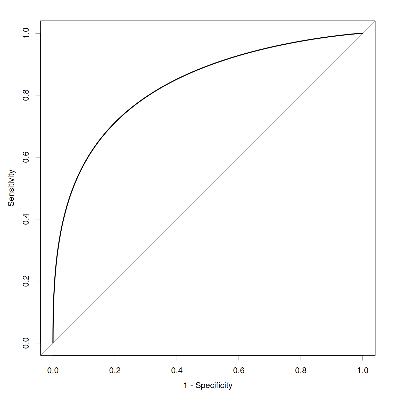
- The AUC is \(.84\). AUC indicates the probability that a randomly selected case has a higher test result than a randomly selected control. Thus, the probability is \(84\%\) that a randomly selected passenger who survived had a higher predicted probability of survival (based on the prediction model) than a randomly selected passenger who died. The AUC of \(.84\) indicates that the prediction model was moderately accurate in terms of discrimination.
- Calibration plot:
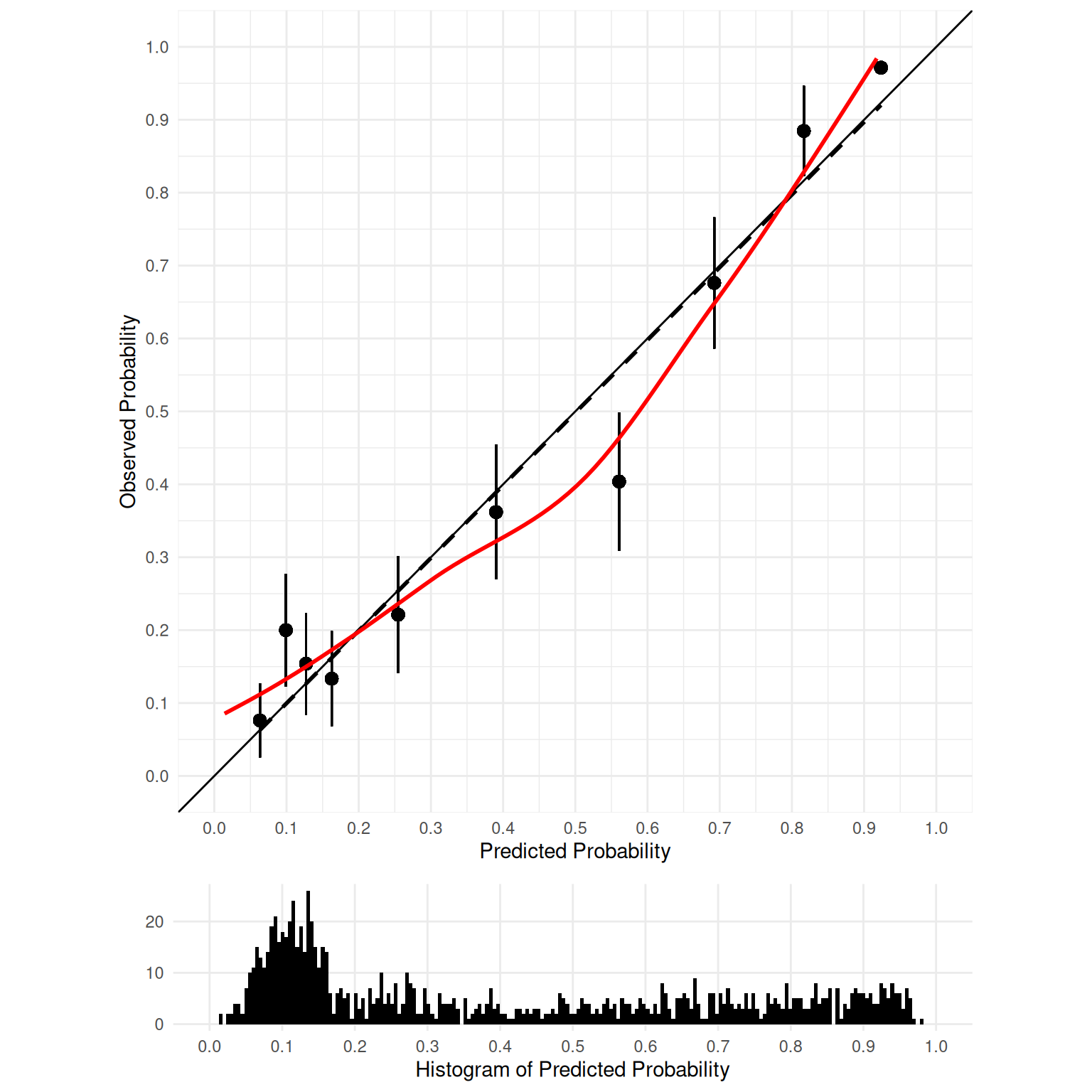
In general, the predictions are well-calibrated. There is not significant miscalibration according to Spiegehalter’s \(z\) \((0.31, p = .76)\). This is verified graphically in the calibration plot, in which the predicted probabilities fall mostly near the actual/observed probabilities. However, based on the calibration plot, there does appear to be some miscalibration. When the predicted probability of survival was ~60%, the actual probability of survival was lower (~40%). This pattern of miscalibration is known as overprediction, as depicted in Figure 1 of Lindhiem et al. (2020).
The 2x2 prediction matrix is below:
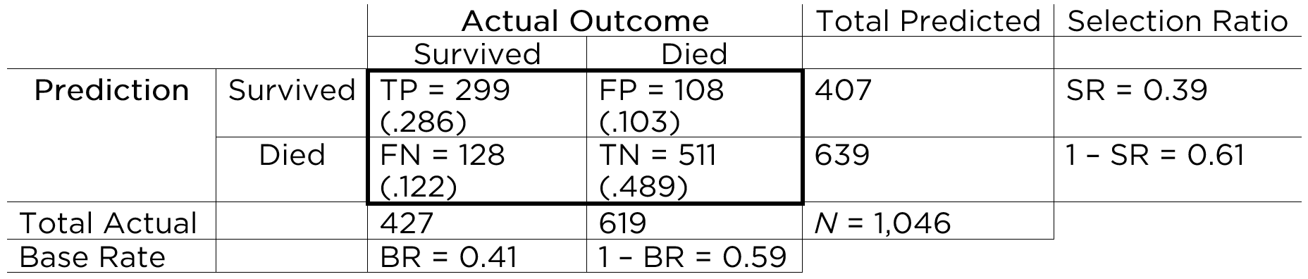
- Selection ratio: \(.39\)
- Base rate: \(.41\)
- Percent accuracy: \(77\%\)
- Percent accuracy by chance: \(52\%\)
- Percent accuracy predicting from the base rate: \(59\%\)
- Relative improvement over chance (ROIC): \(.51\)
- Relative improvement over predicting from the base rate: \(.22\)
- Sensitivity (true positive rate [TPR]): \(.70\)
- Specificity (true negative rate [TNR]): \(.83\)
- False negative rate (FNR): \(.30\)
- False positive rate (FPR): \(.17\)
- Positive predictive value (PPV): \(.73\)
- Negative predictive value (NPV): \(.80\)
- False discovery rate (FDR): \(.27\)
- False omission rate (FOR): \(.20\)
- Diagnostic odds ratio: \(11.05\)
- Youden’s J statistic: \(.53\)
- Balanced accuracy: \(.76\)
- \(F_1\) score: \(0.72\)
- Matthews correlation coefficient (MCC): \(.53\)
- Positive likelihood ratio: \(4.01\)
- Negative likelihood ratio: \(0.36\)
- \(d'\) sensitivity: \(1.46\)
- \(A\) (non-parametric) sensitivity: \(0.83\)
- \(\beta\) bias: \(1.35\)
- \(c\) bias: \(0.21\) aa. \(b\) (non-parametric) bias: \(1.30\) ab. Miscalibration (mean difference between predicted and observed values): \(0.16\) ac. Information gain: \(0.21\)
Predicting from the base rate would have a percent accuracy of \(59\%\). So, the predictions increase the percent accuracy by \(18\%\). If you raise the selection ratio (i.e., predict more people survived) sensitivity will increase whereas specificity will decrease. If you lower the selection ratio, specificity will increase and sensitivity will decrease.
The utility ratio is \(0.25\). The overall utility (\(U_\text{overall}\)) of the cutoff is \(0.41\). The cutoff with the highest overall utility is \(0.266\).
-
The cutoff that optimizes each of the following criteria:
- Youden’s J statistic: \(0.556\)
- Closest to the top left of the ROC curve: \(0.391\)
- Percent accuracy: \(0.618\)
- Percent accuracy by chance: 1 (i.e., predicting from the base rate—that nobody will survive)
- Relative improvement over chance (ROIC): \(.017, .023, .027, .031, .032, .035, .035, .035, .038, .039\)
- Relative improvement over predicting from the base rate: \(.618\)
- Sensitivity (true positive rate [TPR]): 0 (i.e., predicting that everyone will survive will minimize false negatives)
- Specificity: 1 (i.e., predicting that nobody will survive will minimize false positives)
- Positive predictive value (PPP): \(0.875\)
- Negative predictive value (NPV): \(0.017, 0.023, 0.027, 0.031, 0.032, 0.035, 0.035, 0.035, 0.038, 0.039\)
- Diagnostic odds ratio: \(0.875\)
- Balanced accuracy: \(0.556\)
- \(F_1\) score: \(0.391\)
- Matthews correlation coefficient (MCC): \(0.618\)
- Positive likelihood ratio: \(0.875\)
- Negative likelihood ratio: \(0.017, 0.023, 0.027, 0.031, 0.032, 0.035, 0.035, 0.035, 0.038, 0.039\)
- Miscalibration (mean difference between predicted and observed values): \(0.017–0.085\)
- \(d'\) sensitivity: \(0.833\)
- \(A\) (non-parametric) sensitivity \(0.316\)
- \(\beta\) bias \(0.017, 0.023, 0.027, 0.031, 0.032, 0.035, 0.035, 0.035, 0.038, 0.039, 0.979\)
- \(c\) bias \(0.387\)
- \(b\) (non-parametric) bias \(0.017\)
- Overall utility: \(0.266\)
- Information gain: \(0.631\)
- Based on negative predictive value (i.e., the probability of no disease given a negative test), the probability that you actually had the coronavirus is less than 1 in 100 \((.006)\).
- Based on positive predictive value (i.e., the probability of disease given a positive test), the probability that your friend actually had the coronavirus is less than 50% \((.49)\).
- The problem with your friend’s logic is that your friend is assuming they have the antibodies when chances are more likely that they do not.
- Your friend is likely demonstrating the fallacy of base rate neglect.
- A positive test on a screening device is hard to interpret in this situation because of the low base rate. “Even with a very accurate test, the fewer people in a population who have a condition, the more likely it is that an individual’s positive result is wrong.” For more info, see here: https://www.scientificamerican.com/article/coronavirus-antibody-tests-have-a-mathematical-pitfall/ (archived at https://perma.cc/GL9F-EVPH)
According to Bayes’ theorem, the probability that you have the disease is \(24.75\%\). For more info, see here: https://www.scientificamerican.com/article/what-is-bayess-theorem-an/ (archived at https://perma.cc/GM6B-5MEP)
- According to Bayes’ theorem, the probability that you have the virus after testing positive on Test A is \(4.6\%\).
- According to Bayes’ theorem, the updated probability that you have the virus after testing positive on both Tests A and B is \(43.3\%\).
9.14 Session Info
R version 4.6.1 (2026-06-24)
Platform: x86_64-pc-linux-gnu
Running under: Ubuntu 24.04.4 LTS
Matrix products: default
BLAS: /usr/lib/x86_64-linux-gnu/openblas-pthread/libblas.so.3
LAPACK: /usr/lib/x86_64-linux-gnu/openblas-pthread/libopenblasp-r0.3.26.so; LAPACK version 3.12.0
locale:
[1] LC_CTYPE=C.UTF-8 LC_NUMERIC=C LC_TIME=C.UTF-8
[4] LC_COLLATE=C.UTF-8 LC_MONETARY=C.UTF-8 LC_MESSAGES=C.UTF-8
[7] LC_PAPER=C.UTF-8 LC_NAME=C LC_ADDRESS=C
[10] LC_TELEPHONE=C LC_MEASUREMENT=C.UTF-8 LC_IDENTIFICATION=C
time zone: UTC
tzcode source: system (glibc)
attached base packages:
[1] grid stats graphics grDevices utils datasets methods
[8] base
other attached packages:
[1] knitr_1.51 rmarkdown_2.31 tinytex_0.60
[4] here_1.0.2 MOTE_1.2.2 caret_7.0-1
[7] lattice_0.22-9 ggrepel_0.9.8 car_3.1-5
[10] carData_3.0-6 msir_1.4 ggpubr_1.0.0
[13] gridExtra_2.3.1 uroc_0.1.0 PredictABEL_1.2-4
[16] ResourceSelection_0.3-6 rms_8.1-1 Hmisc_5.2-6
[19] ROCR_1.0-12 pROC_1.19.0.1 viridis_0.6.5
[22] viridisLite_0.4.3 magrittr_2.0.5 lubridate_1.9.5
[25] forcats_1.0.1 stringr_1.6.0 dplyr_1.2.1
[28] purrr_1.2.2 readr_2.2.0 tidyr_1.3.2
[31] tibble_3.3.1 ggplot2_4.0.3 tidyverse_2.0.0
[34] petersenlab_1.2.3
loaded via a namespace (and not attached):
[1] RColorBrewer_1.1-3 rstudioapi_0.19.0 jsonlite_2.0.0
[4] TH.data_1.1-5 farver_2.1.2 nloptr_2.2.1
[7] vctrs_0.7.3 minqa_1.2.8 base64enc_0.1-6
[10] rstatix_1.0.0 polynom_1.4-1 htmltools_0.5.9
[13] polspline_1.1.25 broom_1.0.13 Formula_1.2-5
[16] parallelly_1.48.0 htmlwidgets_1.6.4 plyr_1.8.9
[19] sandwich_3.1-1 zoo_1.8-15 lifecycle_1.0.5
[22] iterators_1.0.14 pkgconfig_2.0.3 Matrix_1.7-5
[25] R6_2.6.1 fastmap_1.2.0 future_1.70.0
[28] rbibutils_2.4.1 PBSmodelling_2.70.2 digest_0.6.39
[31] colorspace_2.1-2 rprojroot_2.1.1 labeling_0.4.3
[34] timechange_0.4.0 mgcv_1.9-4 abind_1.4-8
[37] compiler_4.6.1 bit64_4.8.2 withr_3.0.3
[40] htmlTable_2.5.0 S7_0.2.2 backports_1.5.1
[43] DBI_1.3.0 psych_2.6.5 ggsignif_0.6.4
[46] animation_2.8 lava_1.9.2 MASS_7.3-65
[49] quantreg_6.1 ModelMetrics_1.2.2.2 tools_4.6.1
[52] pbivnorm_0.6.0 foreign_0.8-91 otel_0.2.0
[55] future.apply_1.20.2 nnet_7.3-20 glue_1.8.1
[58] quadprog_1.5-8 nlme_3.1-169 checkmate_2.3.4
[61] cluster_2.1.8.2 reshape2_1.4.5 generics_0.1.4
[64] recipes_1.3.3 gtable_0.3.6 tzdb_0.5.0
[67] class_7.3-23 data.table_1.18.4 hms_1.1.4
[70] foreach_1.5.2 pillar_1.11.1 vroom_1.7.1
[73] mitools_2.4 splines_4.6.1 bit_4.6.0
[76] survival_3.8-6 SparseM_1.84-2 tidyselect_1.2.1
[79] mix_1.0-13 reformulas_0.4.4 stats4_4.6.1
[82] xfun_0.60 hardhat_1.4.3 timeDate_4052.112
[85] stringi_1.8.7 yaml_2.3.12 boot_1.3-32
[88] evaluate_1.0.5 codetools_0.2-20 tcltk_4.6.1
[91] cli_3.6.6 rpart_4.1.27 xtable_1.8-8
[94] Rdpack_2.6.6 lavaan_0.6-21 Rcpp_1.1.2
[97] globals_0.19.1 XML_3.99-0.23 parallel_4.6.1
[100] MatrixModels_0.5-4 gower_1.0.2 mclust_6.1.3
[103] listenv_1.0.0 lme4_2.0-1 mvtnorm_1.4-1
[106] ipred_0.9-15 prodlim_2026.03.11 scales_1.4.0
[109] crayon_1.5.3 rlang_1.3.0 multcomp_1.4-30
[112] mnormt_2.1.2 Please note that the areas in the figure are not drawn to scale; otherwise, some regions would be too small to include text.↩︎