I want your feedback to make the book better for you and other readers. If you find typos, errors, or places where the text may be improved, please let me know. The best ways to provide feedback are by GitHub or hypothes.is annotations.
Opening an issue or submitting a pull request on GitHub: https://github.com/isaactpetersen/Principles-Psychological-Assessment
Adding an annotation using hypothes.is.
To add an annotation, select some text and then click the
symbol on the pop-up menu.
To see the annotations of others, click the
symbol in the upper right-hand corner of the page.
23 Repeated Assessments Across Time
23.1 Overview of Repeated Measurement
Repeated measurement enables examining within-person change in constructs. Relating within-person change in a construct to within-person change in another construct provides a stronger test of causality compared to simple bivariate correlations. Identifying that within-person change in construct X predicts later within-person change in construct Y does not necessarily indicate that X causes Y but it provides stronger evidence consistent with causality than a simple bivariate association between X and Y. As described in Section 5.3.1.3.3.1, there are three primary reasons a correlation between X and Y does not necessarily mean that X causes Y: First, the association could reflect the opposite direction of effect, where Y actually causes X. Second, the association could reflect the influence of a third variable that influences both X and Y (i.e., a confound). Third, the association might be spurious.
If you find that within-person changes in sleep predict later within-person changes in mood, that is a stronger test of causality because (a) it demonstrates temporal precedence; it attenuates the possibility that the association is due to the opposite direction of effect; and (b) it accounts for all time-invariant confounds that differ between people (e.g., birth order) because the association is examined within the individual. That is, the association examines whether the person’s mood is better when they get more sleep compared to when that same person gets less sleep. The association could still be due to time-varying confounds, but you can control for specific time-varying confounds if you measure them.
Repeated measurement also enables examination of the developmental timing of effects and sensitive periods. Furthermore, repeated measures designs are important for tests of mediation, which are tests of hypothesized causal mechanisms.
Repeated measurement involves more complex statistical analysis than cross-sectional measurement because multiple observations come from the same person, which would violate assumptions of traditional analyses that the observations (i.e., the residuals) are independent and uncorrelated. Mixed-effects modeling (i.e., mixed modeling, multilevel modeling, hierarchical linear modeling) and other analyses, such as structural equation modeling, can handle the longitudinal dependency or nesting of repeated measures data.
Repeated measurement can encompass many different timescales, such as milliseconds, days, or years.
23.1.1 Comparison of Approaches
Research designs can be compared in terms of their internal validity—the extent to which we can be confident about causal inferences. A cross-sectional association is depicted in Figure 23.1:
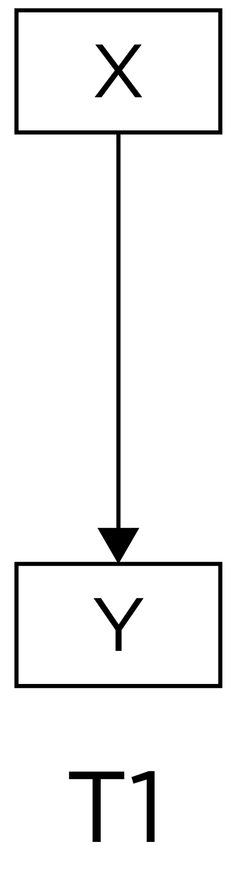
Among observational/correlational research designs, cross-sectional designs tend to have the weakest internal validity. That is, if we observe a cross-sectional association between \(X\) and \(Y\), we have little confidence that \(X\) causes \(Y\). Consider a lagged association, which is a slightly better approach:
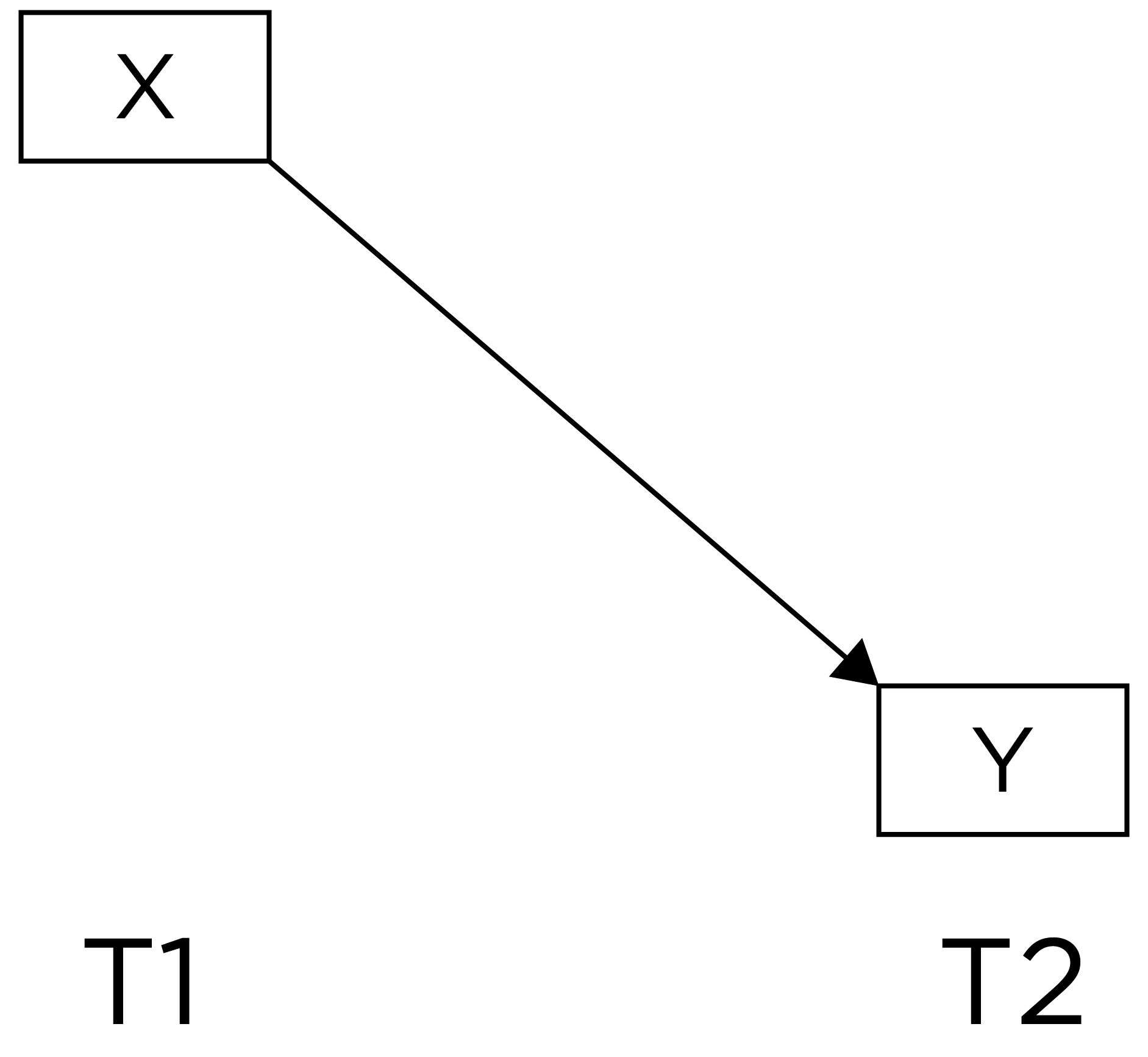
A lagged association has somewhat better internal validity than a cross-sectional association because we have greater evidence of temporal precedence—that the influence of the predictor precedes the outcome because the predictor was assessed before the outcome and it shows a predictive association. However, part of the association between the predictor with later levels of the outcome could be due to prior levels of the outcome that are stable across time. Thus, consider an even stronger alternative—a lagged association that controls for prior levels of the outcome:
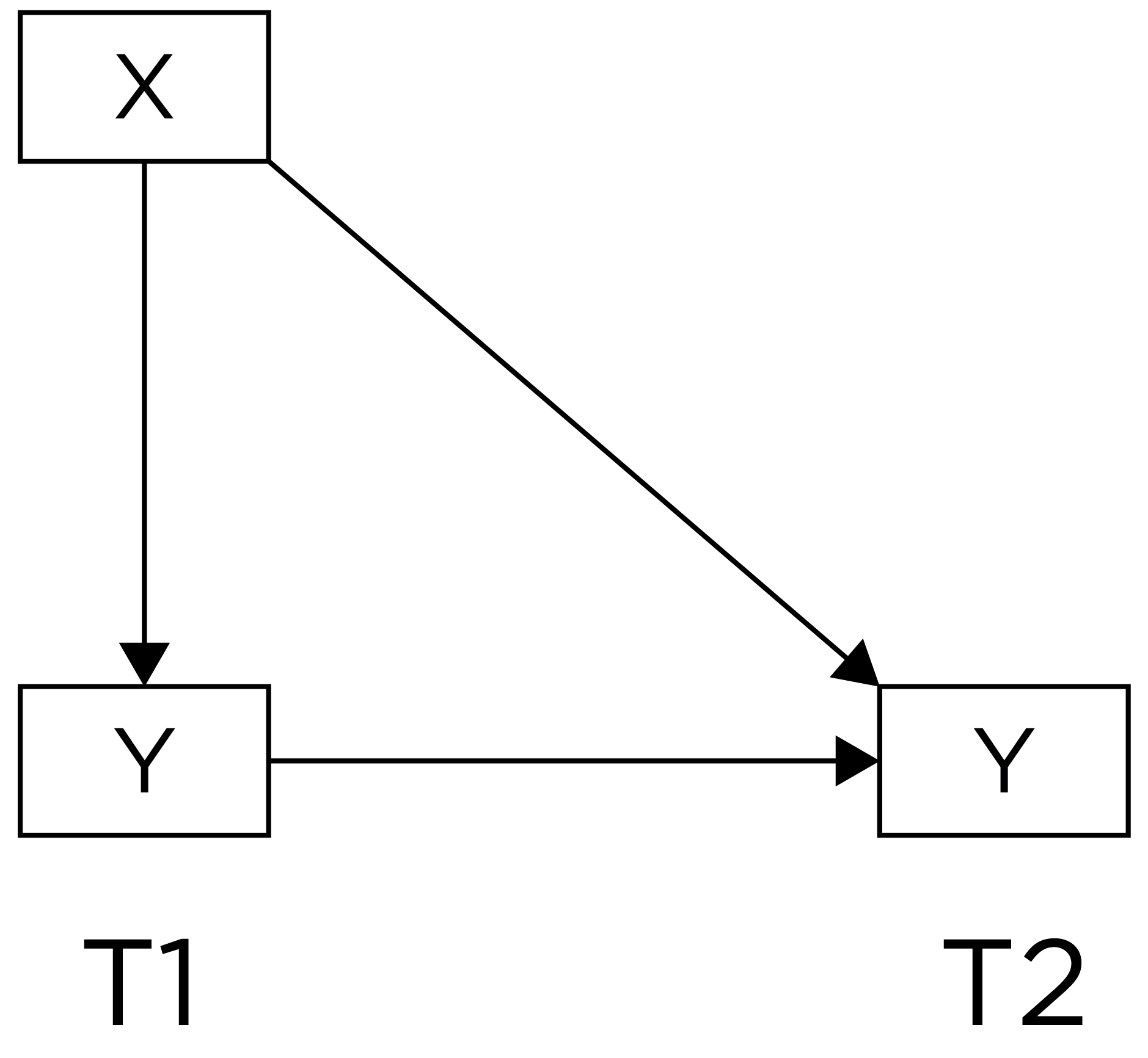
A lagged association controlling for prior levels of the outcome has better internal validity than a lagged association that does not control for prior levels of the outcome. When we control for prior levels of the outcome in the prediction, we are essentially predicting (relative) change. Predicting change provides stronger evidence consistent with causality because it uses the individual as their own control and controls for many time-invariant confounds. However, consider an even stronger alternative—lagged associations that control for prior levels of the outcome and that simultaneously test each direction of effect:
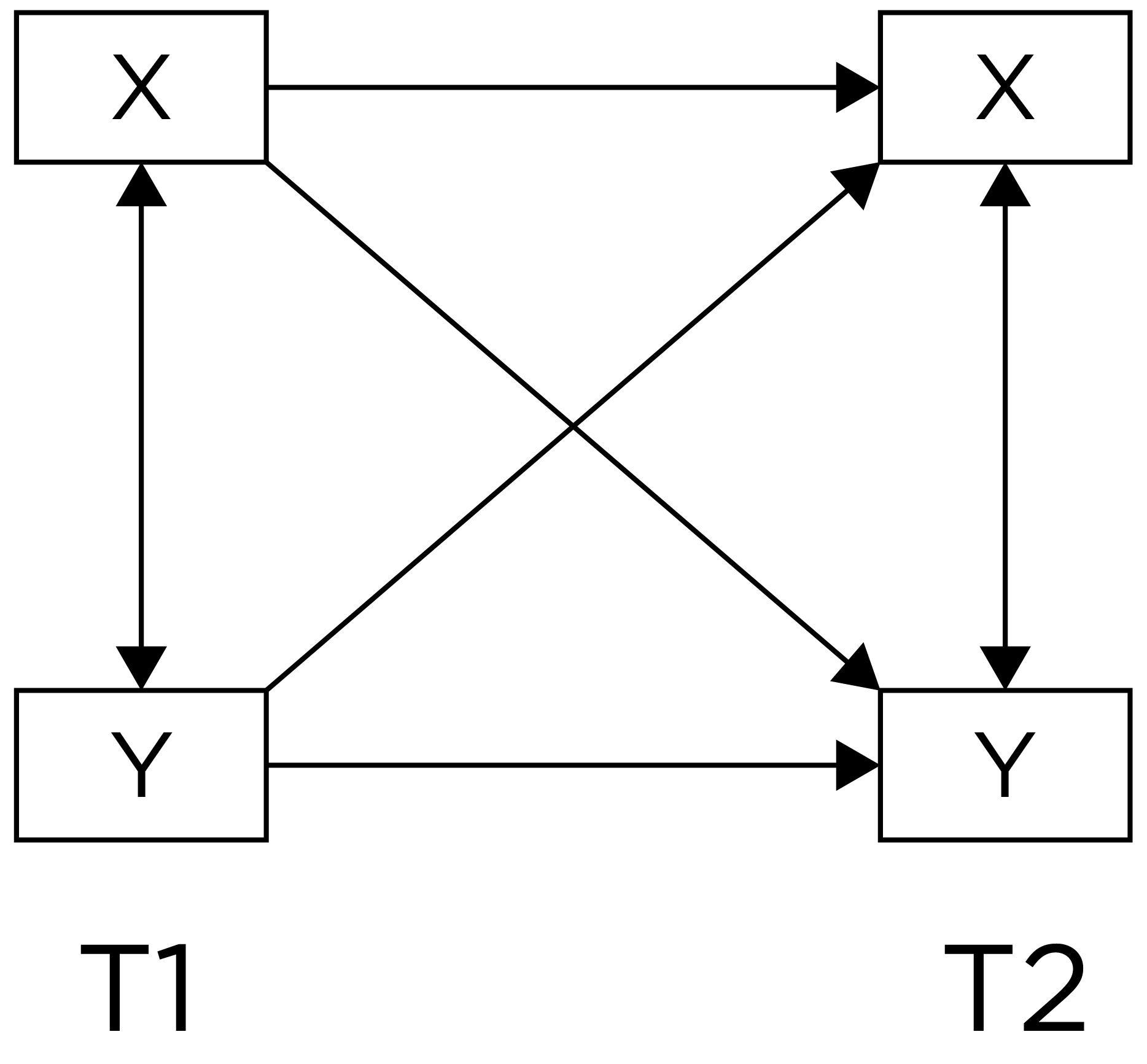
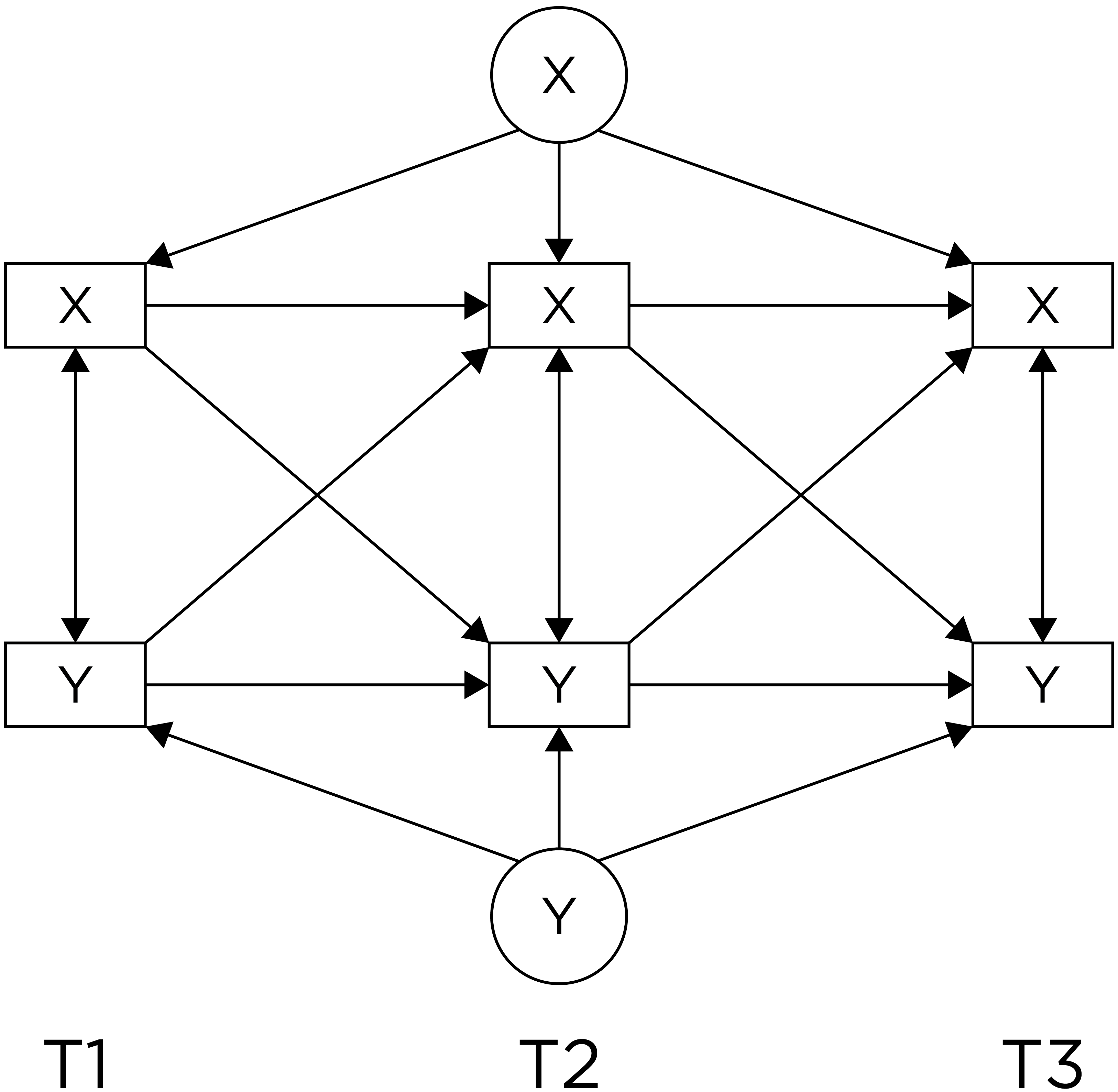
Lagged associations that control for prior levels of the outcome and that simultaneously test each direction of effect provide the strongest internal validity among correlational/observational designs, especially when examining whether within-person changes in the predictor predict later within-person changes in the outcome (and vice versa). Such a design can help better clarify which among the variables is the chicken and the egg—which variable is more likely to be the cause and which is more likely to be the effect. Or, if there are bidirectional, transactional effects, what the magnitude of each direction of effect are. The cross-lagged panel model and dual latent change score model are examples of models that include lagged associations that control for prior levels of the outcome and that simultaneously test each direction of effect. However, consider an even stronger model—lagged associations that control for prior levels of the outcome and for random intercepts and that simultaneously test each direction of effect:
Some researchers have called into question the cross-lagged panel model (Berry & Willoughby, 2017; Hamaker et al., 2015). A stronger alternative may be a cross-lagged model that controls for stable between-person differences (i.e., random intercepts) (Hamaker et al., 2015). This is known as a random intercepts cross-lagged panel model.
23.2 Examples of Repeated Measurement
Below are some examples of repeated measurement.
23.2.1 Alcohol Timeline Followback
A clinically relevant example of repeated measurement is the Alcohol Timeline Followback, published by Sobell & Sobell (2008). The Alcohol Timeline Followback is a method for retrospectively assessing the quantity of alcohol consumption on a daily basis. It provides retrospective estimates of people’s drinking using a calendar of the number of drinks consumed each day. The time frame can vary from 30 days to 360 days. The participant is given detailed instructions to enhance the accuracy of recall and reporting of their behavior.
Moreover, a specific definition is provided of what counts as a drink. The measure is intended to provide a detailed record of patterns of alcohol use to guide treatment and assess treatment outcome. The measure provides many summary statistics and norms are available.
The measure has several clinical uses. First, it can provide personalized feedback to the client regarding their drinking behavior compared to the population as part of enhancing their motivation to change, in a motivational interviewing framework. Second, the measure can help identify high- and low-risk periods for a client to help them prevent relapse.
Because the measure provides detailed information with norms, it can be more useful than global estimates of drinking derived from less structured clinical interviews. The detailed instructions help respondents remember more accurately, so the clinician or researcher can examine how people’s substance abuse influences other processes like parenting.
23.2.2 Ambulatory Assessment
We discussed ambulatory assessment in Section 20.2.4.1. Ambulatory assessment includes an array of methods used to study people in their natural environment. There is a proliferation of smartphone apps for ambulatory assessment. And the ambulatory assessments often, because of their temporal resolution, provide repeated measurements.
For instance, Carpenter et al. (2016) depicted the examination, during a drinking episode, of self-reported drinking in relation to physiological indices including skin temperature, heart rate, breathing rate, physical activity, and in relation to self-reported sadness and mood dysregulation. The self-reported indices were assessed on various intervals (e.g., every 15 minutes) and upon various events (e.g., when they take a drink). However, the physiological indices were assessed continuously from moment to moment. These different timescales pose challenges for how to examine them in relation to each other.
Matthews et al. (2016) provided an example of how they developed an ambulatory assessment using a smartphone app to assess the dynamic process of bipolar disorder. Regularity of social rhythms is disrupted in bipolar disorder, so the authors developed an app to help assess social rhythms. The authors used a participatory design in which they involved the patients in the development of the app to ensure it worked well for them. The app tracked the occurrence and timing of daily events, such as getting out of bed, starting your day, having dinner, and going to bed. It also passively detected daily events (“social rhythms”) with many sensors on the smartphone using information from the light, accelerometer, and microphone of the smartphone. And the app used a machine learning algorithm to estimate level of physical activity and social interaction.
23.3 Test Revisions
An important part of repeated measurements deals with test revisions. Tests are revised over time. Some test revisions are made to be consistent with improvements in the understanding of the construct. Other test revisions are made to make the norms more up-to-date. For instance, the Weschler Adult Intelligence Scale has multiple versions (WAIS-3, WAIS-IV, etc.). There are important considerations when dealing with test revisions.
When you assess people at different times, whether the same people at multiple time points (such as in a longitudinal study) or different people at different times, challenges may result in comparing scores across time. There can be benefits of keeping the same measure across ages or across time for comparability of scores. However, it is not necessarily good to use the same measure across ages or at different times merely for the sake of mathematical comparability of scores. If a measure was revised to improve its validity or if a measure is not valid at particular ages, it may make sense to use different measures across ages or across time. You would not want to use a measure at a given age if it is not valid at that age. Likewise, it does not make sense to use an invalid measure at a later time point if a more valid version becomes available, even if it was used at an earlier time point. That is, even if a measure’s scores are mathematically comparable across ages or time, they may not be conceptually comparable across ages or time. If different measures are used across ages or across time, there may be ways to link scores from the different measures to be on the same scale, as described in Section 23.9.4.1.3.
One interesting phenomenon of time-related changes in scores is the Flynn effect, in which the population scores on intelligence tests rise around 3 points every decade. That is, intelligence, as measured by tests of cognitive abilities, increases from generation to generation. Test revisions can hide effects like the Flynn effect if we just keep using score transformations instead of raw scores.
To observe a person’s (or group’s) growth, it is recommended to use raw scores rather than standardized scores that are age-normed, such as T scores, z scores, standard scores, and percentile ranks (Moeller, 2015). Age-normed scores prevent observing growth at the person level or at the group level (e.g, changes in means or variances over time). T scores (\(M = 50\), \(SD = 10\)), z scores (\(M = 0\), \(SD = 1\)), and standard scores (\(M = 100\), \(SD = 15\)) have a fixed mean and standard deviation. Percentile ranks have a fixed range (0–100).
23.4 Change and Stability
A key goal of developmental science is to assess change and stability of people and constructs. Stability is often referred to in a general way. For instance, you may read that intelligence and personality show “stability” over time. However, this is not a useful way of describing the stability of people and/or constructs because stability is not one thing. There are multiple types of stability, and it is important to refer to the types of stability considered.
Types of stability include, for instance, stability of level, rank order (individual differences), and structure. Stability of level refers to whether people show the same level on the construct over time. For example, stability of level considers whether people stay the same in their level of neuroticism across childhood to adulthood. Stability of people’s level is evaluated with the coefficient of repeatability.
Mean-level stability refers to whether the mean level stays the same across time. For example, mean-level stability considers whether the population average stays the same in their level of neuroticism across childhood to adulthood. Mean-level stability is evaluated by examining mean-level age-related differences; for instance, with a t-test or ANOVA, or by examining whether the construct is associated with age.
Rank-order stability refers to whether individual differences stay the same across time. For instance, rank-order stability considers whether people who have higher neuroticism than their peers as children also tend to have higher neuroticism than their peers as adults. Rank-order stabiliy is examined by examining the association of people’s level at T1 with people’s level at T2 (e.g., correlation coefficient or regression coefficent).
Stability of structure considers whether the structure of the construct stays the same across ages. For instance, stability of structure considers whether personality is characterized by the same five factors across ages (i.e., openness, conscientiousness, extraversion, agreeableness, and neuroticism). Stability of structure is examined using longitudinal factorial invariance.
People and constructs can show stability in some types and not others. For instance, although intelligence and personality show relative stability in structure and rank-order, they do not show absolute stability in level. Even though individual differences in intelligence and personality show relative stability, people tend to change across time in their absolute level of intelligence and various personality factors across ages. For instance, neuroticism decreases in later adulthood. Examining age-normed scores would preclude identifying mean-level change because age-normed scores have a fixed mean. Moreover, examining a strong correlation of intelligence and personality scores across time merely indicates that individual differences show relative stability; it does not indicate whether individuals show absolute stability in level.
23.5 Assessing Change
There are many important considerations for assessing change, that is changes in a person’s level on a construct across time. There is a key challenge in assessing change between two time points. If a person’s score differs between two time points, how do you know that the differences across time reflect a person’s true change in their level on the construct rather than measurement error, such as regression to the mean? Regression to the mean occurs if an extreme observation on a measure at time 1 (T1) more closely approximates the person’s mean at later time points, including time 2 (T2). For instance, clients with high levels of symptomatology tend to get better with the mere passage of time, which has been known as the self-righting reflex.
23.5.1 Inferring Change
The inference of change is strengthened to the extent that:
- the magnitude of the difference between the scores at the two time points is large (i.e., a large effect size)
- the measurement error (unreliability) at both time points is small
- the measure has the same meaning and is on a comparable scale at each time point (i.e., the measure’s scores show measurement invariance across time)
- evidence suggests that the differences across time are not likely to be due to potential confounds of change such as practice effects, cohort effects, and time-of-measurement effects.
Measurement error can be reduced by combining multiple measures of a construct into a latent variable, such as in structural equation modeling (SEM) or item response theory (IRT).
To detect change, it is important to use measures that are sensitive to change. For instance, the measures should not show range restriction owing to ceiling effects or floor effects.
At the individual level, it is common to infer that a person’s level changed from T1 from T2 if the magnitude of their change is greater than the smallest real difference. However, just because a person (or a group) changed in their level on the construct does not necessarily mean that the change is meaningful. Thus, it is also important to consider the effect size of the change and whether the change is greater than the minimal clinically important difference (MCID).
23.5.2 Potential Confounds of Change
Potential confounds of change include practice effects, cohort effects, and time-of-measurement effects.
23.5.2.1 Practice Effects
It is important to consider the potential for practice or retest effects (Hertzog & Nesselroade, 2003). Practice/retest effects occur to the extent that a person improves on a task assessed at multiple time points for reasons due to the repeated assessment rather than true changes in the construct. That is, a person is likely to improve on a task if they complete the same task at multiple time points, even if they are not changing in their level on the construct. Practice and retest effects are especially likely to be larger the closer in time the retest is to the prior testing. Improvement in scores across time might not reflect people’s true change in the construct; thus, you might not be able to fairly compare people’s scores who have completed the task different numbers of times.
In sum, the ages and frequency of assessment should depend on theory.
23.5.2.2 Cohort Effects
It is also important to consider the potential for cohort effects (Hertzog & Nesselroade, 2003). Cohorts often refer to birth cohorts—people who were born at the same time (e.g., the same year). Cohorts tend to have some similar experiences at similar ages, including major events (e.g., 9/11 terrorist attacks, assassination of John F. Kennedy, bombing of Pearl Harbor) and economic or socio-political climates (e.g., the Great Depression, coronavirus pandemic, Cold War, World War II). These collective differences in the different experiences between different cohorts may lead to apparent age-related differences between cohorts that are not actually due to age differences per se, but rather to differences in the experiences between the cohorts.
23.5.2.3 Time-of-Measurement Effects
It is also important to consider time-of-measurement effects. For instance, people’s general anxiety may be higher, on average, during the coronavirus pandemic. Thus, some apparent age-related differences might be due to the time of measurement (i.e., a pandemic) rather than age.
23.5.3 When and How Frequently to Assess
Key questions arise in terms of when (at what ages or times) and how often to assess the construct. If the measurement intervals are too long, you might miss important change in between. If the measurement intervals are too frequent, differences might reflect only measurement error. The Nyquist theorem provides guidance in terms of how frequently to assess a construct. According to the Nyquist theorem, in order to accurately reproduce a signal, you should sample it at twice the highest frequency you wish to detect. For instance, to detect a 15 Hz wave, you should sample it at least at 30 Hz (Hertz means times per second). Thus, the frequency of assessment should be as frequent as, if not more frequent than, the highest frequency of change you seek to observe.
23.5.4 Difference Scores
As described in Section 4.5.8, difference scores (also called change scores) can have limitations because they can be less reliable than each of the individual measures that compose the difference score. The reliability of individual differences in change scores depends on the extent to which: (a) the measures used to calculate the change scores are reliable, and (b) the variability of true individual differences in change is large (Rogosa & Willett, 1983)—that is, there are true individual differences in change.
23.5.4.1 Superior Approaches to Difference Scores
There are several options that are better than traditional difference scores or change scores. Instead of difference scores, use autoregressive cross-lagged models, latent change score models, or growth curve models.
23.5.4.1.1 Autoregressive Cross-Lagged Models
Autoregressive cross-lagged models (aka cross-lagged panel models) can be fit in path analysis or SEM. Cross-lagged panel models examine relative change in a variable, that is, change in individual differences in the variable, but not changes in level on the variable. Such a model allows examining whether one variable predicts relative change in another variable. The cross-lagged panel model tests whether individuals with low levels of X relative to others experience subsequent rank-order increases in Y (Evans & Shaughnessy, 2024; Orth et al., 2021). By contrast, the random-intercepts cross-lagged panel model tests whether, when individuals experience lower-than-their-own usual levels of X, they experience subsequent increases in Y relative to their usual level (Evans & Shaughnessy, 2024; Orth et al., 2021). As an example of a cross-lagged panel model, I conducted a collaborative study that examined whether language ability predicts later behavior problems controlling for prior levels of behavior problems—that is, whether language ability predicts a person’s change in behavior problems relative to the change among other people in the sample (Petersen et al., 2013; Petersen & LeBeau, 2021). Cross-lagged panel models predict relative (rank-order) change, not absolute change in level. For tests of absolute change, models such as change score models or growth curve models are necessary.
23.5.4.1.2 Latent Change Score Models
Latent change score models can be fit in SEM. Unlike autoregressive cross-lagged models, latent change score models examine absolute change—that is, people’s changes in level. With latent change score models, you can examine change in latent variables that reflect the common variance among multiple measures. Latent variables are theoretically error-free (at least of random error), so latent change scores can be perfectly reliable, unlike traditional difference scores, whose reliability is strongly influenced by the measurement unreliability of the specific measures that compose them. Latent change score models are described by Kievit et al. (2018).
23.5.4.1.3 Growth Curve Models
Growth curve models can be fit in mixed-effects modeling or SEM. Growth curve models require three or more time points to be able to account for measurement error in terms of the shape of a linear trajectory. Growth curve models examine absolute change, i.e., changes in level. Growth curve models include an intercept (starting point) and slope (amount of change), but you can model other nonlinear forms of change as well, such as quadratic, logistic, etc. with more time points. Growth curve models correct for measurement error in the shape of the person’s trajectory. In addition, growth curve models can examine risk and protective factors as predictors of the intercepts and slopes. For instance, in collaboration, I examined risk and protective factors that predict the development of externalizing problems (Petersen et al., 2015).
23.5.5 Nomothetic Versus Idiographic
The approaches described above (autoregressive cross-lagged models, latent change score models, and growth curve models) tend to be nomothetic in nature. That is, they are interested in examining group-level phenomena and assume that all people come from the same population and can be described by the same parameters of change. That is, they assume a degree of homogeneity, even though they allow each person to differ in their intercept and slope. This nomothetic (population) approach differs from an idiographic (individual) approach. In clinical work, we are often interested in making inferences or predictions at the level of the individual person, consistent with an idiographic approach. But fully ignoring the population estimates is unwise because they tend to be more accurate than individual-level judgments. Further, individual-level predictions may not generalize to the population. Nomothetic modeling approaches can be adapted to examine change for different subgroups if there are theoretically different populations. Approaches that examine different subgroups include group-based trajectory models, latent class growth models, and growth mixture models (Fontaine & Petersen, 2017; van der Nest et al., 2020).
For instance, Moffit (1993, 2006b, 2006a) created the developmental taxonomy of antisocial behavior with the support of these approaches. Moffitt identified one subgroup that showed very low levels of antisocial behavior across the lifespan, which she labeled the “low” group. She identified one subgroup that showed antisocial behavior only in childhood, which she labeled the “childhood-limited” group. She hypothesized that the antisocial behavior among the childhood-limited group was influenced primarily by genetic factors and the early environment. She identified another subgroup that showed antisocial behavior only in adolescence, which she labeled the “adolescent-limited”group. She hypothesized that the antisocial behavior among the adolescent-limited group was largely socially mediated. She identified another subgroup that showed antisocial behavior across the lifespan, which she labeled the “life-course persistent” group. She hypothesized that the “life-course persistent” group reflected neuropsychological deficits.
Idiographic approaches for personalized modeling of psychopathology are described by Wright & Woods (2020). An example of an approach that combines an idiographic (person-centered) approach with a nomothetic (population) approach to understand change is the group iterative multiple model estimation (GIMME) model, as described by Beltz et al. (2016) and Wright et al. (2019). The GIMME model is a data-driven approach to identifying person-specific time-series models. The approach first identifies the associations among constructs that replicate across most participants. The group-level associations are then used as a starting point for identifying person-specific associations. Thus, the GIMME model provides an approach for developing personalized time-series models. The choices on which model to use depend on the research question and should be guided by theory.
23.5.6 Structural Equation Modeling
Structural equation modeling (SEM) allows multiple dependent variables. This provides a key advantage in longitudinal designs, such that two constructs can each be represented by a dependent variable that is predicted by the other. If examining changes in two constructs in the context of SEM, you could examine for instance whether one precedes the other in prediction, to better understand which might cause which and to help tease apart the chicken and the egg. For instance, in collaboration, I found that low language ability predicts later behavior problems stronger than behavior problems predict later language ability, suggesting that, if they are causally related, that language ability is more likely to have a causal effect on behavior problems than the reverse (Petersen et al., 2013).
23.5.7 Attrition and Systematic Missingness
Rates of attrition in longitudinal studies can be substantial and missingness is often not completely at random. There is often selective and systematic attrition. For example, attrition often differs as a function of socioeconomic status and other important factors. It is important to use approaches that examine and account for systematic missingness. It can be helpful to use full-information maximum likelihood (FIML) in SEM to make use of all available data. Multiple imputation is another approach that can be helpful for dealing with missingness. With multiple imputation, you can use predictors that might account for missingness, such as socioeconomic status and demographic factors. You can help account for practice effects with planned missingness designs in which participants are randomly assigned to receive or not receive a given measurement occasion.
23.5.8 Measurement Invariance
Just like measurement or factorial invariance can be tested and established across genders, races, ethnicities, cultures, etc. to ensure measurement equivalence, it can also be tested across ages or times. The goal is to establish longitudinal measurement invariance, i.e., measurement invariance across ages, so that you know that you are assessing the same construct over time in a comparable way so that you know that differences across time reflect true change. To examine longitudinal measurement invariance, you can use SEM or IRT. In SEM, you could examine whether measures have the same intercepts, factor loadings, and residuals across ages. In IRT, you could examine whether items show differential item functioning, versus whether they show the same difficulty and discrimination across ages.
But there are times when we would expect a construct would, theoretically, fail to show longitudinal factorial invariance, as in the case of heterotypic continuity, described in Section 23.9.
23.6 Types of Research Designs
Schaie (1965), Baltes (1968), and Schaie & Baltes (1975) proposed various types of research designs, in terms of the various combinations of age, period (i.e., time of measurement), and cohort. Age refers to a person’s chronological age at the time of measurement. Period refers to the time of measurement (e.g., April 12, 2014 at 7:53 AM). Cohort refers to a person’s time (e.g., year) of birth (e.g., 2003). If you know two of these (e.g., age and period), you can determine the third (e.g., cohort). Here are the types of research designs based on combinations of age, period, and cohort:
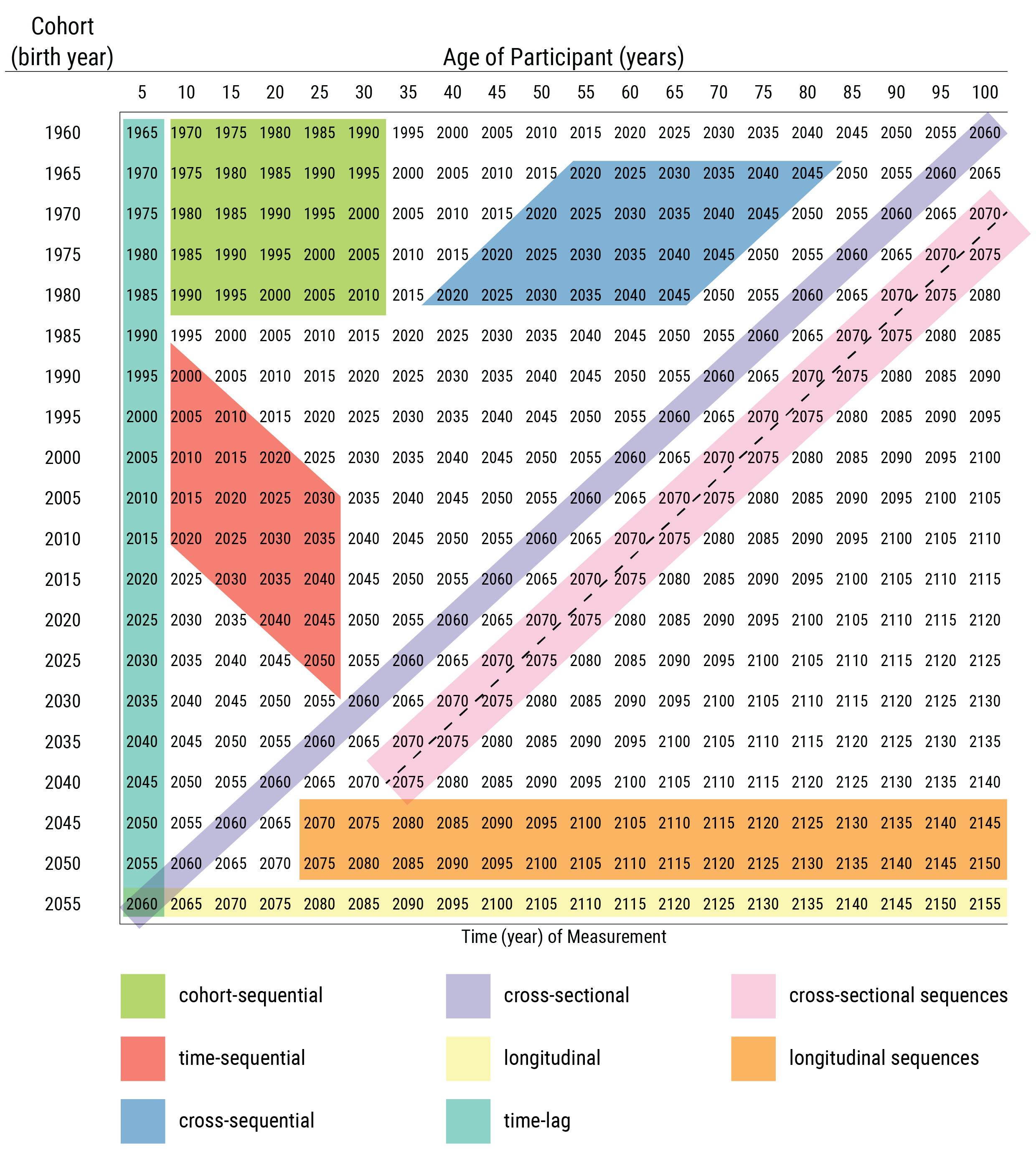
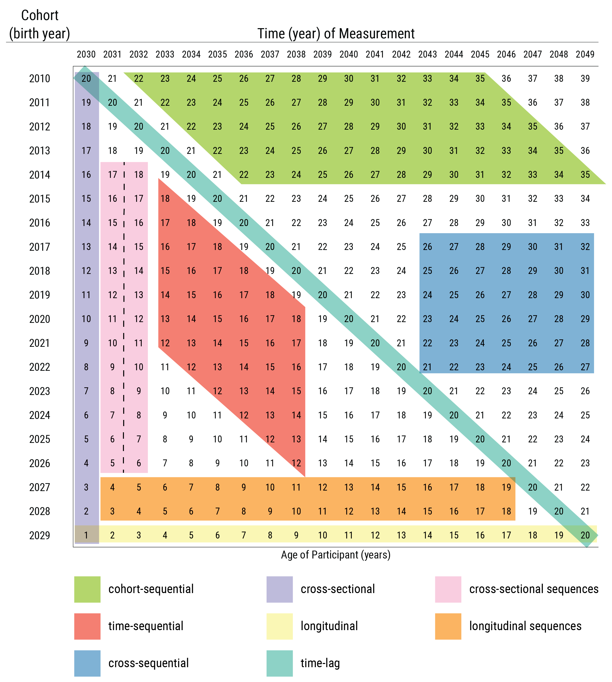
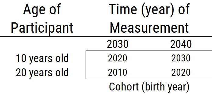
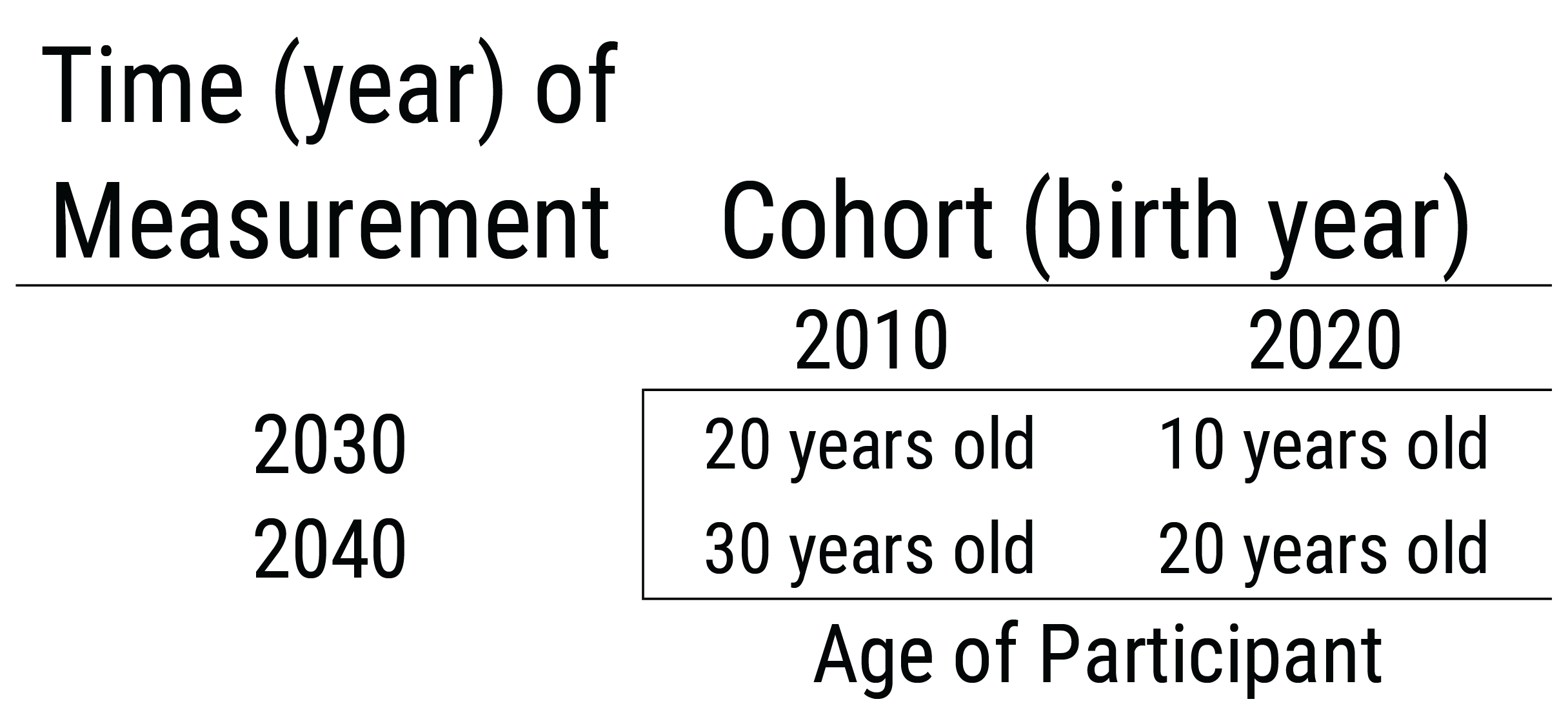
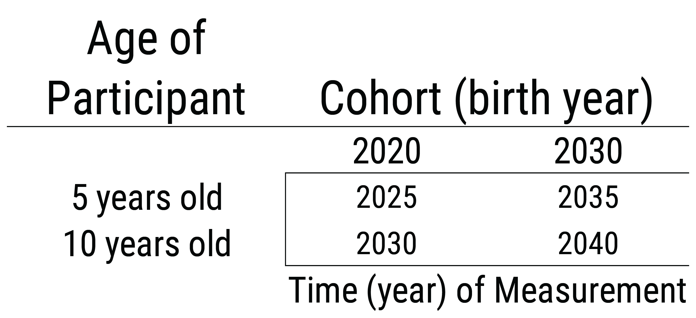
These research designs are depicted by age and cohort in Figure 23.6 and by time of measurement and cohort in Figure 23.7. Although the depictions of cohort-sequential and cross-sequential designs differ from the depictions by Schaie (2005) (i.e., they are reversed), they are consistent with contemporary definitions of these designs (Little, 2013; Masche & Dulmen, 2004; Whitbourne, 2019).
23.6.1 Cross-Sectional Design
A cross-sectional design involves multiple participants, often spanning different ages, assessed at one time of measurement. A cross-sectional design is a single factor design, where the researcher is interested in comparing effects of one factor: age. However, in a cross-sectional design, cohort (i.e., birth year) is confounded with age differences. Thus, observed age-related differences could reflect cohort differences rather than true age differences. Additionally, sampling differences at each age could yield non-comparable age groups.
Cross-sectional designs are thus limited in their ability to describe developmental processes including change and stability over time. Any age-related differences are confounded with cohort differences and are strongly influenced by between age-group sampling variability. Cross-sectional studies are useful for preliminary data on validity of measures for the age groups, and for examining whether the age differences are in the expected direction. Cross-sectional studies are less costly and time-consuming than longitudinal studies. Therefore, they are widely used and provide a useful starting point.
However, findings from cross-sectional studies can differ from findings examining the same people over time, which violates the convergence assumption. In cross-sectional studies, the convergence assumption is the assumption that cross-sectional age differences and longitudinal age changes converge onto a common trajectory. However, it has been shown, for example, that cross-sectional studies over-estimate age-related cognitive declines compared to following the same people over time in a longitudinal study (Ackerman, 2013).
23.6.2 Cross-Sectional Sequences Design
A cross-sectional sequences design involves successive cross-sectional studies of different participants at different times of measurement. In a cross-sectional sequences design, cohort and time-of-measurement are confounded with age differences. Thus, observed age-related differences could reflect cohort differences or time-of-measurement differences rather than true age differences. This poses challenges for using cross-sectional sequences to estimate age-related changes due to time-related effects such as the Flynn effect.
23.6.3 Time-Lag Design
A time-lag design involves participants from different cohorts assessed at the same age. The time-lag design is a single factor design: the researcher specifies one factor: cohort. However, time of measurement is confounded with cohort. Thus, any cohort differences could reflect different times of measurement.
23.6.4 Longitudinal Design
A longitudinal design involves following the same participants over time. The single-cohort longitudinal design is a single factor design: the researcher specifies one factor: age. However, in a single-cohort longitudinal design, cohort and time of measurement are confounded with age. Thus, any observed changes with age could be due to time-of-measurement effects or cohort effects (instead of people’s true change).
23.6.5 Longitudinal Sequences Design
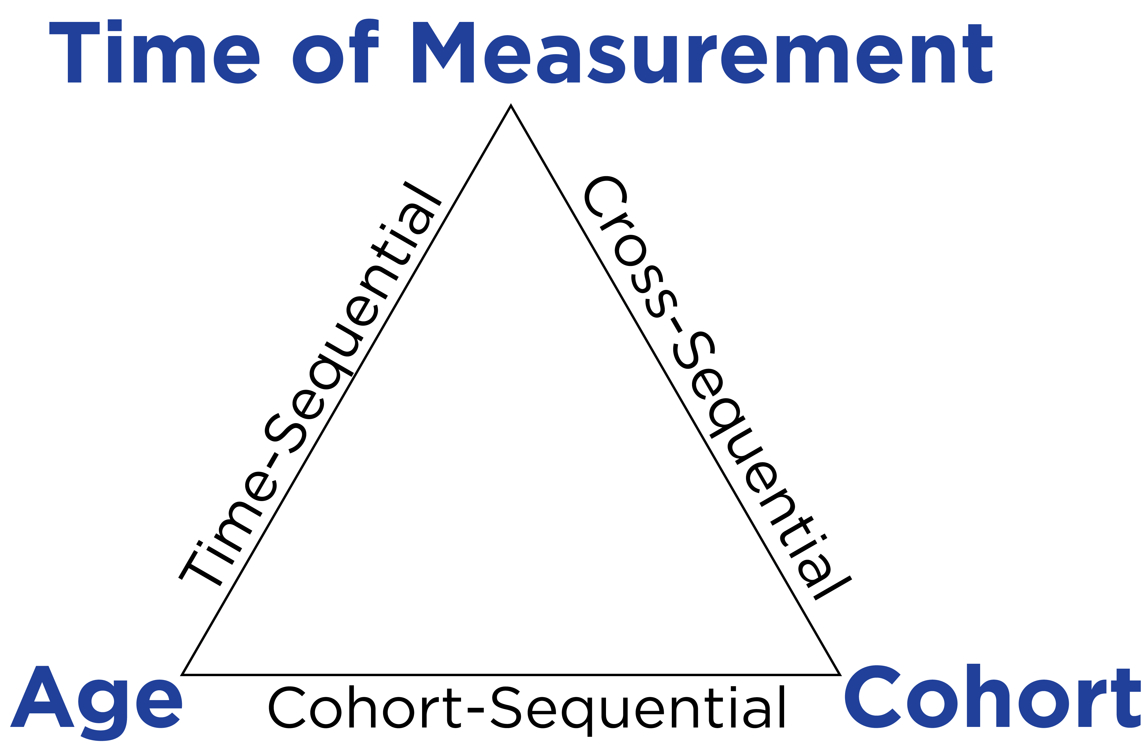
A longitudinal sequences design involves following multiple cohorts across time. There are three types of longitudinal sequences designs: time-sequential, cross-sequential, and cohort-sequential designs. The three types of longitudinal sequences are depicted in Figure 23.8 as a function of which two factors are specified by the researcher.
23.6.5.1 Time-Sequential Design
A time-sequential design is depicted in Figure 23.9. In a time-sequential design, multiple age groups are assessed at multiple times (Whitbourne, 2019). It is a repeated cross-sectional design, with some participants followed longitudinally. Additional age groups are added to a time-lag design, with some of the participants assessed at more than time point. In other words, the age range is kept the same and is repeatedly assessed (with only some participants being repeatedly assessed). The two factors a researcher specifies in a time-sequential design are age and time of measurement. A time-sequential design can be helpful for identifying age differences while controlling for time-of-measurement differences, or for identifying time-of-measurement differences while controlling for age differences. However, cohort effects are confounded with the interaction of age and time of measurement (Whitbourne, 2019). Thus, observed differences as a function of age or time of measurement could reflect cohort effects.
23.6.5.2 Cross-Sequential Design
A cross-sequential design is depicted in Figure 23.10. In a cross-sequential design, multiple cohorts are assessed at multiple times (Whitbourne, 2019). It is a cross of a cross-sectional and longitudinal design. It starts as a cross-sectional study with participants from multiple cohorts, and then all participants are followed longitudinally (typically across the same duration). It is also called an accelerated longitudinal design. The two factors a researcher specifies in a cross-sequential design are time of measurement and cohort. A cross-sequential design can be helpful for identifying cohort differences while controlling for time-of-measurement differences, or for identifying time-of-measurement differences while controlling for cohort differences. However, age differences are confounded with the interaction between cohort and time of measurement. Thus, observed differences as a function of cohort or time of measurement could reflect age effects.
23.6.5.3 Cohort-Sequential Design
A cohort-sequential design is depicted in Figure 23.11. In a cohort-sequential design, multiple cohorts are assessed at multiple ages (Whitbourne, 2019). It starts multiple cohorts at the same age and then follows them longitudinally (typically across the same duration). It is like starting a longitudinal study at the same age over and over again. The two factors a researcher specifies in a cohort-sequential design are age and cohort. A cohort-sequential design can be helpful for identifying age differences while controlling for cohort differences, or for identifying cohort differences while controlling for age differences. However, time-of-measurement effects are confounded with the interaction of age and cohort (Whitbourne, 2019). Thus, observed differences as a function of age or cohort could reflect time-of-measurement effects.
23.7 Using Sequential Designs To Make Developmental Inferences
Which research design you select should depend on which change function you are most interested in: age, cohort, or time of measurement. However, age is not the only metric for development; time after a transition (e.g., school entry, quitting smoking) or an exposure (e.g., puberty onset) can also be an important time metric. There are many other potential metrics of time for studying development.
To have greater confidence that age-related differences reflect true change (development) rather than effects of cohort or time of measurement, we would conduct all three sequential designs. To the extent that the age-related effects in the time-sequential and cohort-sequential designs are stronger than the cohort- and time-of-measurement effects in the cross-sequential design, we have confidence that the observed age-related differences reflect development (Whitbourne, 2019). Moreover, there is an entire set of analytic approaches, known as age-period-cohort analysis (Yang & Land, 2013), whose goal is to disentangle the effects of age, period, and cohort.
23.8 Stability Versus Continuity
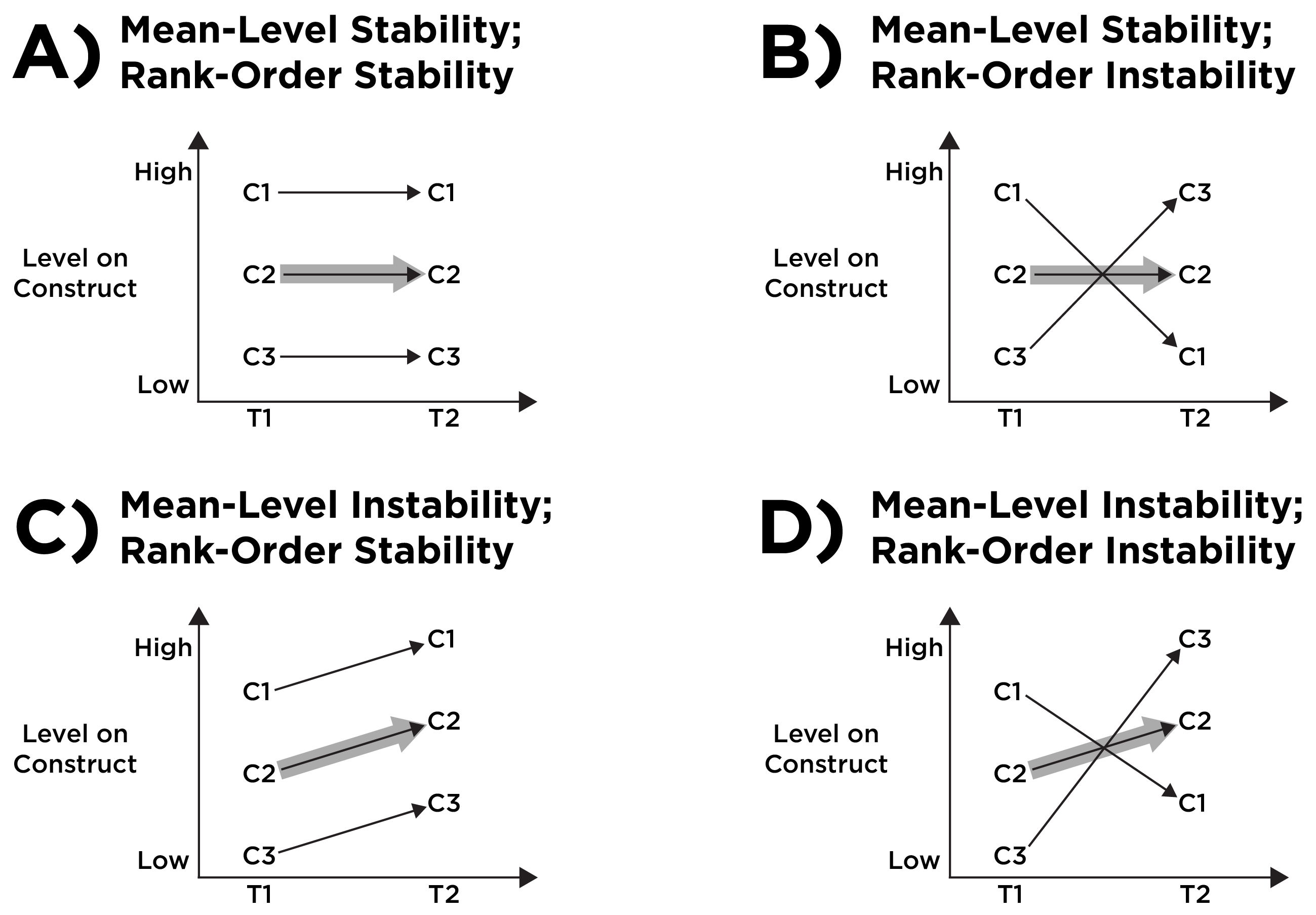
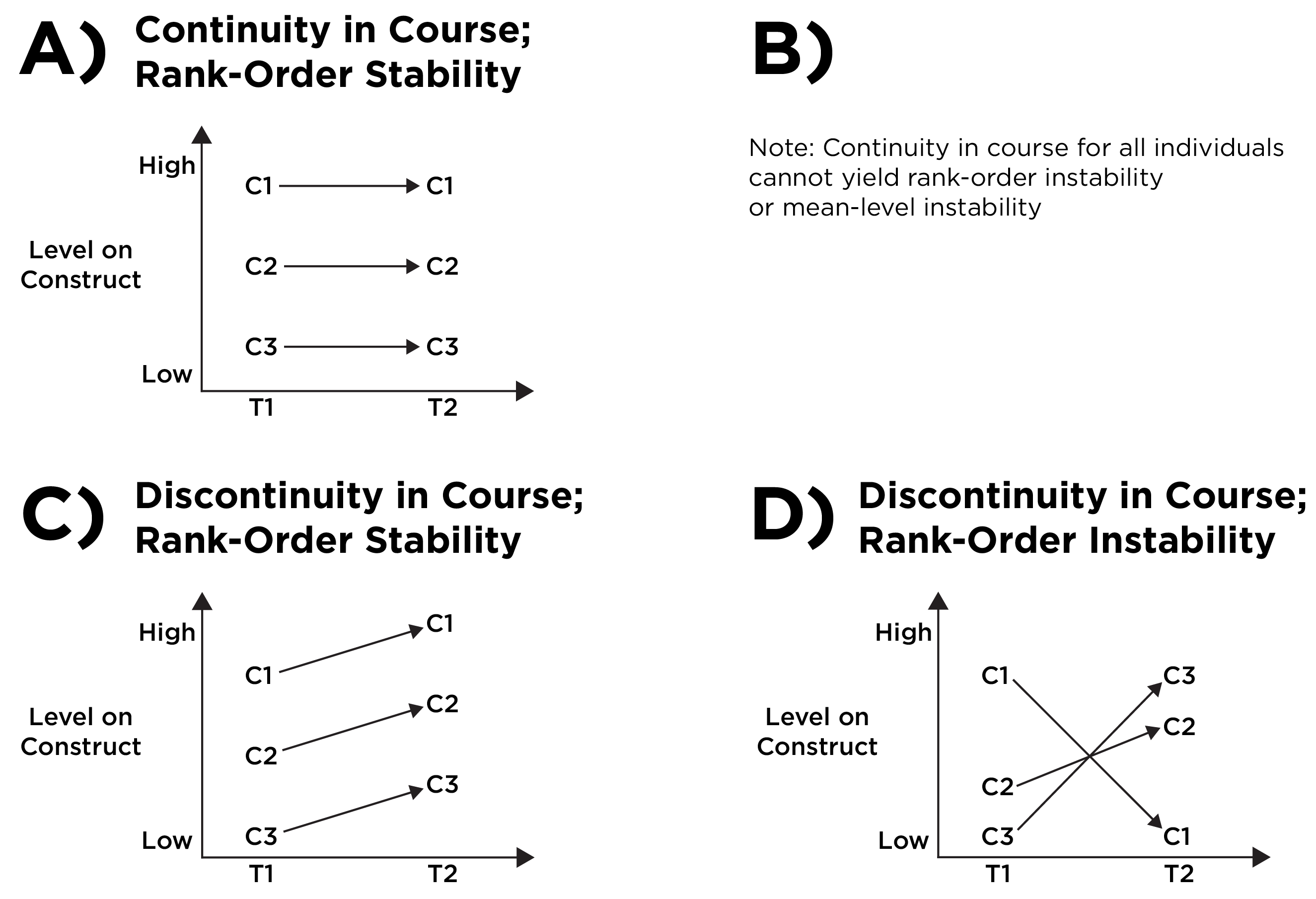
Continuity addresses the trajectory of development within individuals. By contrast, stability refers to the maintenance of between-individual or group characteristics (Petersen, 2024; Schulenberg et al., 2014; Schulenberg & Zarrett, 2006). When describing stability or continuity, it is important to specify which aspects of stability (e.g., of mean, variance, or rank order) and continuity (e.g., of causes, courses, forms, functions, or environments) one is referring to. For example, Figure 23.12 depicts the distinction between mean-level stability and rank-order stability; Figure 23.13 depicts the distinction between continuity in course and rank-order stability.
(ref:meanVsRankOrderStabilityCaption) Mean-Level Stability Versus Rank-Order Stability. C1, C2, and C3 are three individual children assessed at two timepoints: T1 and T2. The gray arrow depicts the mean (average) trajectory. (Figure reprinted from Petersen (2024), Figure 1, Petersen, I. T. (2024). Reexamining developmental continuity and discontinuity in the 21st century: Better aligning behaviors, functions, and mechanisms. Developmental Psychology, 60(11), 1992–2007. https://doi.org/10.1037/dev0001657 Copyright (c) American Psychological Association. Used with permission.)
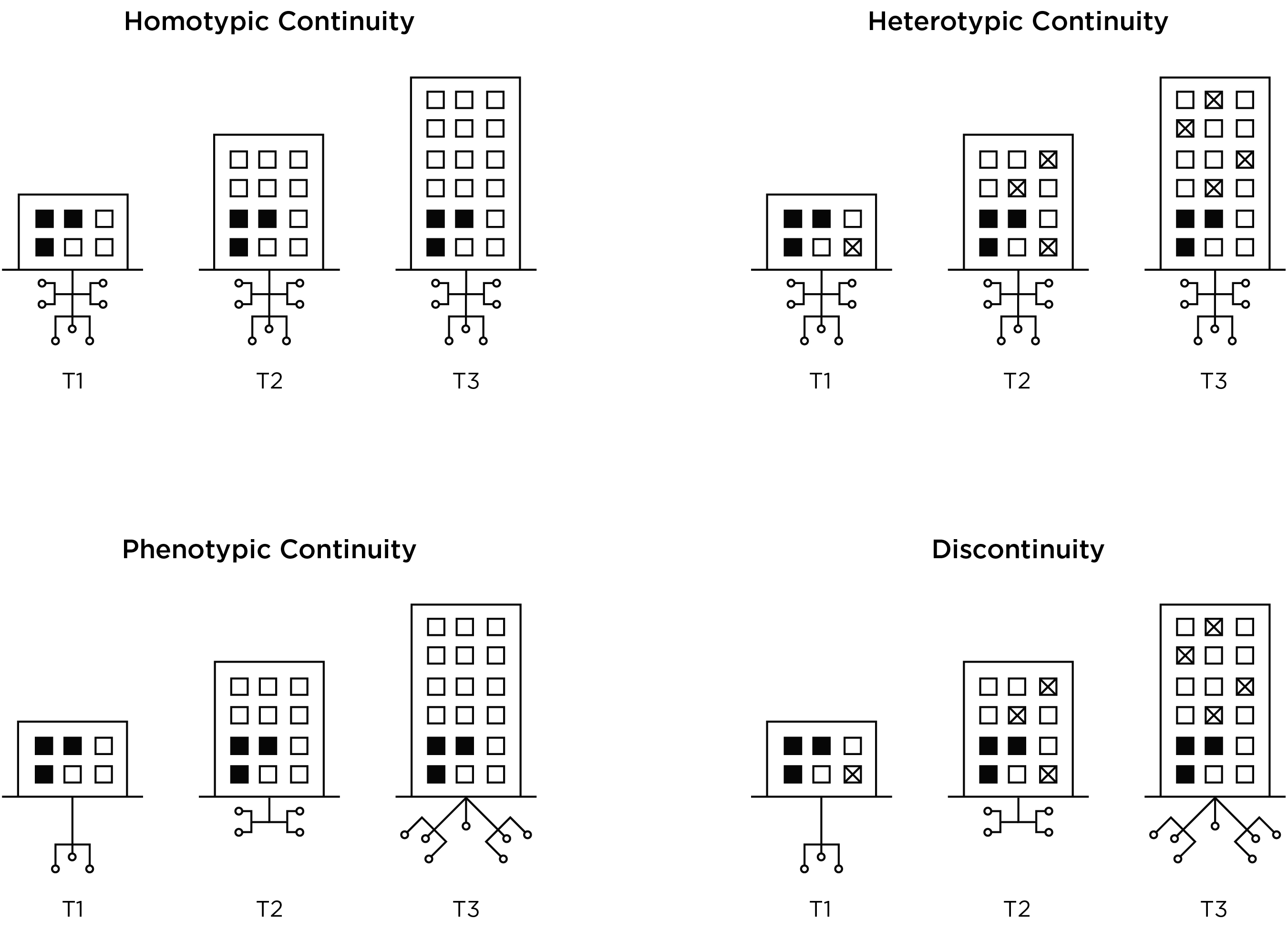
The various types of continuity, including homotypic continuity, heterotypic continuity, and phenotypic continuity, in addition to discontinuity are depicted in Figures 23.14 and 23.15.
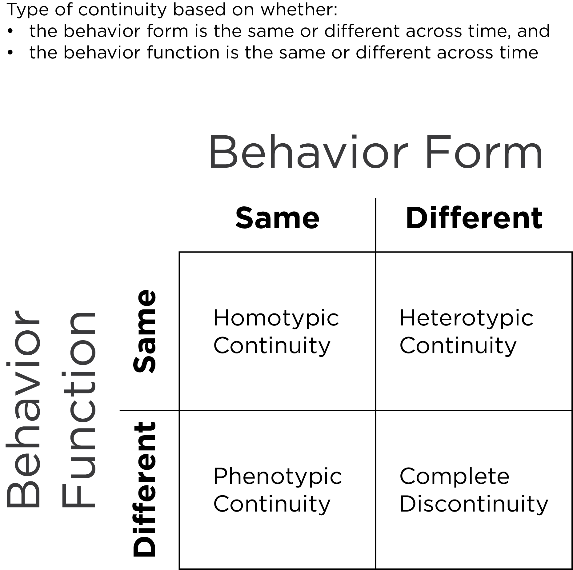
23.9 Heterotypic Continuity
Heterotypic continuity is the persistence of an underlying construct with behavioral manifestations that change across development (Caspi & Shiner, 2006; Cicchetti & Rogosch, 2002; Petersen et al., 2020; Petersen, 2024). Patterson (1993) described antisocial behavior like a chimera. A chimera is a mythical creature with a body of a goat that, with development, grows the head of a lion and then a tail of a snake. Patterson (1993) conceptualized antisocial behavior across development as having an underlying essence of oppositionality that is maintained while adding more mature features with age, including the ability to inflict serious damage with aggression and violence. Other analogies of heterotypic continuity include the change from water to ice or steam, and the metamorphosis of a caterpillar to a butterfly—the same construct shows different manifestations across development.
23.9.1 How to Identify Heterotypic Continuity
Heterotypic continuity can be identified or quantified as changes in the factor structure (i.e., content) of a construct across time. The content of a measure include the facets assessed by a given measure, such as individual behaviors, questionnaire items, or sub-dimensions of a broader construct. The content of the measure can be compared to content of a construct to evaluate the content validity of the measure.
Heterotypic continuity is present to the extent that the content of a construct show cross-time changes in: people’s rank-order stability, the content’s level on the construct, and how strongly the content reflect the construct. Cross-time changes in people’s rank-order stability indicate changes in the degree of stability of individual differences in the construct across time, and are examined with correlation of the content across time.
The content’s level on the construct is similar to the inverse of frequency, prevalence, or base rate of the content. The content’s level on the construct is examined with item difficulty (severity) in IRT or with intercepts in SEM. For example, the item “sets fires” has a higher item severity than the item “argues” because setting fires is less frequent than arguing.
How strongly the content reflect the construct, conceptually is the degree of a content’s construct validity, and is examined with item discrimination in IRT or with factor loadings in SEM. For example, the item “hits others” has a higher item discrimination than “eats ice cream” for the construct of externalizing problems because hitting others is more strongly related to the construct (compared to eating ice cream).
Externalizing problems are an example of a construct that changes in behavioral manifestation with development (Chen & Jaffee, 2015; Miller et al., 2009; Moffitt, 1993; Patterson, 1993; Petersen et al., 2015; Petersen & LeBeau, 2022; Wakschlag et al., 2010). The content of externalizing problems show changes in the magnitude of rank-order stability, changes in the content’s level on the construct, and changes in how strongly the construct reflect the construct. For example, inattention shows increases in the magnitude of rank-order stability with age (Arnett et al., 2012). Drinking alcohol becomes more frequent in adolescence compared to childhood, so its item severity decreases. Threatening other people is more strongly associated with externalizing problems in adolescence than in early childhood (Lubke et al., 2018). Moreover, externalizing content, including disobedience and biting, likely change in meaning with developoment. In childhood, disobedience could be an indicator of externalizing problems. In adulthood, disobedience could serve prosocial functions, including protesting against societally unjust actions, and thus shows weaker construct validity for externalizing problems. In general, in early childhood, externalizing problems often manifest in overt forms, such as physical aggression and temper tantrums. Later in development, externalizing problems tends to manifest in covert forms, such as indirect aggression, relational aggression, and substance use (Miller et al., 2009).
In addition to externalizing problems, other constructs also likely show heterotypic continuity across development. For instance, internalizing problems may show heterotypic continuity (Weems, 2008; Weiss & Garber, 2003) such that anxiety precedes depression (Garber & Weersing, 2010). In addition, somatic complaints such as headaches, stomachaches, and heart pounding are more strongly associated with and more common in those with internalizing problems in childhood than adulthood (Petersen et al., 2018). Other constructs that show heterotypic continuity include inhibitory control (Petersen et al., 2016; Petersen, Bates, et al., 2021), substance use (Schulenberg & Maslowsky, 2009), sleep states (Blumberg, 2013), and temperament (Putnam et al., 2008). In addition, constructs that are typically assessed with different measures across ages also likely show heterotypic continuity, including language ability (Petscher et al., 2018), nonverbal ability (McArdle & Grimm, 2011), working memory (McArdle et al., 2009), and academic skills (Tong & Kolen, 2007). In sum, many constructs likely show heterotypic continuity.
However, it is important rule out potential alternatives to heterotypic continuity, as depicted in Figure 23.16.
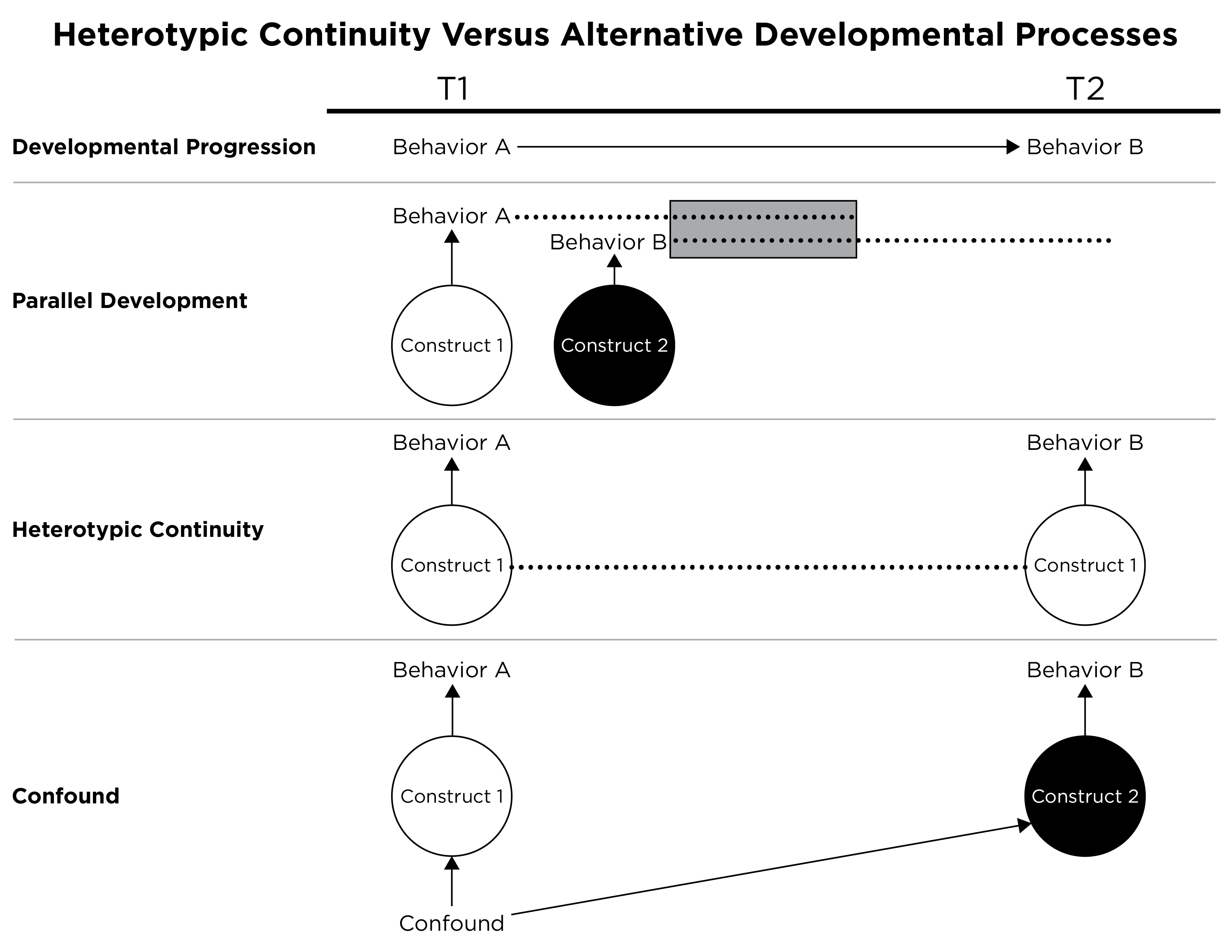
23.9.2 The Problem
Heterotypic continuity poses challenges for longitudinal assessment. According to the maxim, “what we know depends on how we know it”. If a construct changes in manifestation across time, and the measures do not align with the changing manifestation, the scores will not validly assess individual’s growth. Failing to account for heterotypic continuity leads to misidentified trajectories of people’s growth (Chen & Jaffee, 2015; Petersen et al., 2026) and to trajectories that are less able to detect people’s change (Petersen et al., 2018; Petersen, LeBeau, et al., 2021). Thus, it is important that our measurement and statistical schemes account for heterotypic continuity when a construct changes in manifestation across time. These measurement and statistical schemes are discussed below.
23.9.3 Ways to Assess a Construct Across Development
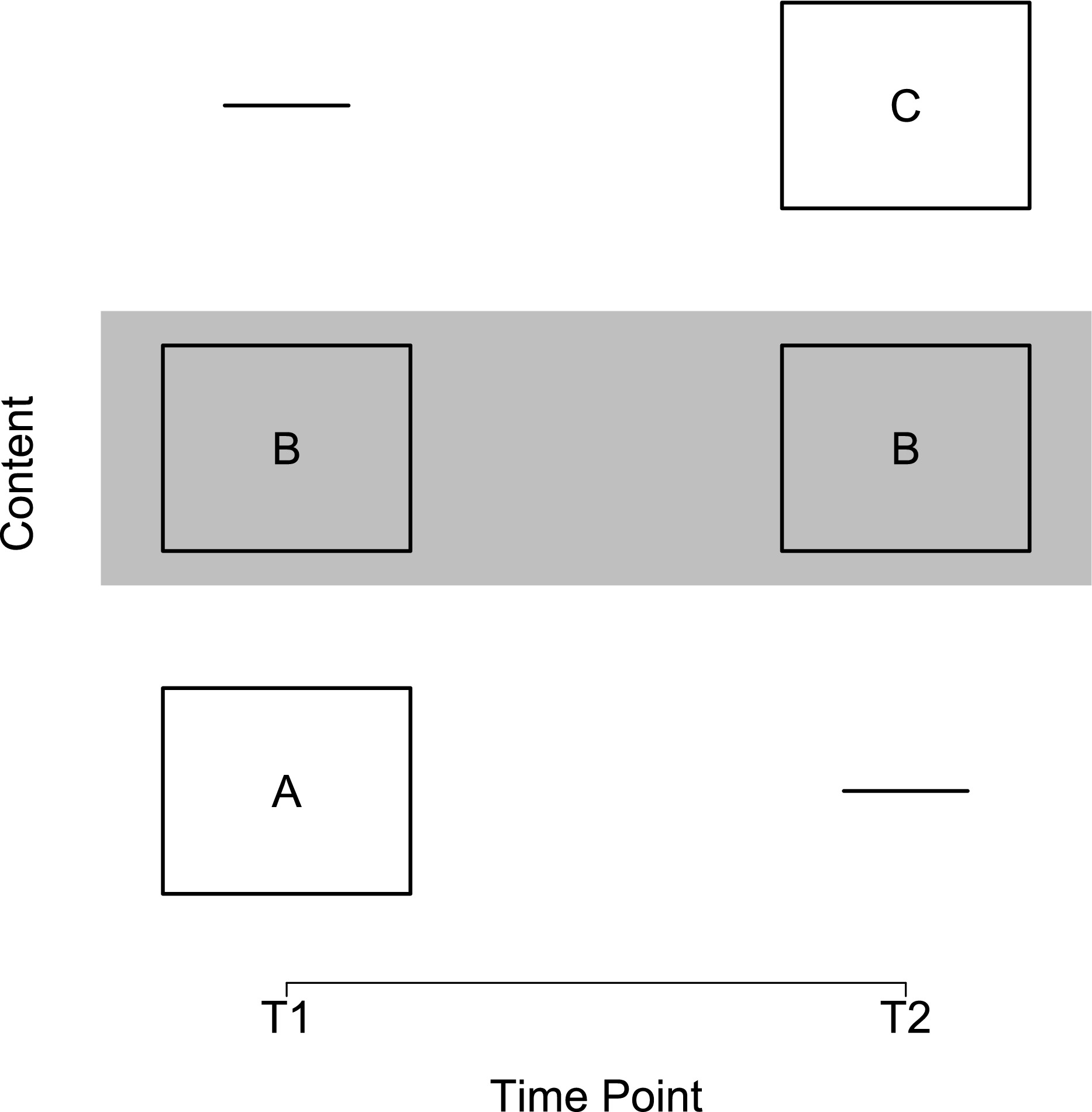
There are three ways of assessing a construct across development:
- All possible content
- Only the common content
- Only the construct-valid content
Assume content A is construct-valid at T1, content B is content-valid at T1 and T2, and content C is content-valid at T2. All possible content would assess: ABC at T1, ABC at T2. Only the common content would assess: B at T1, B at T2. Only the construct-valid content would assess: AB at T1, BC at T2. A depiction of assessing only the construct-valid content is in Figure 23.17.
23.9.3.1 All Possible Content
There are advantages and disadvantages of each. Advantages of using all possible content include that it is comprehensive and allows examining change in each content facet. However, it also has key disadvantages. First, it is inefficient and assesses lots of items. Second, it could assess developmentally inappropriate content. And in the case of heterotypic continuity, it assesses content that lack construct validity, i.e., there are item intrusions.
23.9.3.2 Only the Common Content
Advantages of using only the common content include that it is efficient and may exclude developmentally inappropriate content. Moreover, it permits examining consistent content across ages. However, it also has key disadvantages. First, it results in fewer items and a loss of information. In particular, it may involve a systematic loss of content that reflects very low or very high levels on the construct. Third, and due to the loss of information, it may be less sensitive to developmental change. And in the case of heterotypic continuity, it assesses content that lack content validity because all important facets of the construct are not assessed—i.e., there are item gaps.
23.9.3.3 Only the Construct-Valid Content
There are disadvantages to using only the construct-valid content. First, it is more time-intensive than assessing only the common content. Second, it uses a different measure across time, which can pose challenges to ensuring scores across time are comparable. Nevertheless, the approach has important advantages. First, it is more efficient than using all possible content. Second, it retains content validity and construct validity. And in the case of heterotypic continuity, it is recommended. Developmental theory requires that we account for changes in the construct’s expression!
Many measures are used outside the age range for which they were designed and validated to use. Many measures for children and adolescents are little more than downward extensions of those developed for use with adults (Hunsley & Mash, 2007). Use of the same measure across ages does not ensure measurement equivalence. The problem is that even if the same measure is used across ages, the measure may lack construct validity at some ages. Thus heterotypic continuity may require different measures at different ages to retain construct validity. But then there is the challenge of how to assess change when using different measures across time.
23.9.4 Accounting for Heterotypic Continuity
To account for heterotypic continuity, it is recommended to use different measures across time. Specifically, it is recommended to use (only) the construct-valid content at each age when the content is valid for assessing the construct. To ensure scores are comparable across time, despite the differing measures, it is important to take steps to ensure statistical and theoretical equivalence of scores across time.
23.9.4.1 Ensuring Statistical Equivalence
Historically, there have been various attempts to handle different measures across time to ensure statistical equivalence of scores—i.e., that measures are on the same mathematical metric.
23.9.4.1.1 Age-norming
Age-norming includes standardized scores (e.g., T scores, z scores, standard scores) and percentile ranks. However, as discussed in Section 23.3, standardized scores prevent observing individuals’ or groups’ absolute change over time. Moreover, despite putting scores on the same mathematical metric, they do not ensure scores are on the same conceptual metric. Thus, age-norming is not recommended for putting different measures onto the same score to account for heterotypic continuity and examine individuals’ growth.
23.9.4.1.2 Average or Proportion Scores
Average and proportion scores account for the different numbers of items in each measure. However, average and proportion scores assume that measures do not differ in difficulty or discrimination. Thus, average and proportion scores are not recommended to account for heterotypic continuity and examine individuals’ growth.
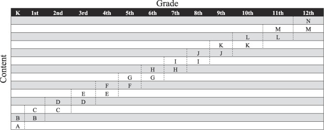
23.9.4.1.3 Developmental Scaling
A third approach to ensure statistical equivalence of measures is developmental scaling, which is also called vertical scaling (see Figure 23.18). In developmental scaling, measures that differ in difficulty and discrimination are placed on the same scale using the common content. The common content set the scale, but all content (including both age-common content and age-differing content) estimate each person’s score on that scale. There are several approaches to developmental scaling, including Thurstone scaling, factor analysis, and IRT.
Thurstone scaling aligns the percentile scores of two measures based on z scores on the common content. It is an observed score approach. An example of Thurstone scaling is provided by Petersen et al. (2018).
Factor analysis allows estimation of a latent variable using different content over time. An example of a factor analysis approach to developmental scaling is provided by Wang et al. (2013). IRT finds scaling parameters that put people’s scores from the different measures on the same metric, and it links the measures’ scales based on the difficulty and discrimination of the common content. Examples of an IRT approach to developmental scaling are provided by Petersen et al. (2018), Petersen, LeBeau, et al. (2021), Petersen & LeBeau (2022), Petersen & LeBeau (2021), and Petersen et al. (2026).
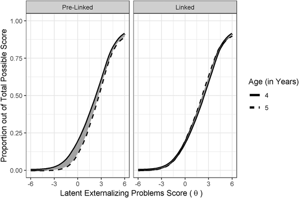
The IRT approach to developmental scaling is depicted in Figure 23.19.
23.9.4.2 Ensuring Theoretical Equivalence
A number of pieces of evidence provide support for the theoretical equivalence of measures. The goal is for the measures to have construct validity invariance—the measure should assess the same construct across time. The content that are assessed at each age should be based on theory. The assessed content should reflect the same construct at relevant ages—i.e., the content should show construct validity at each age they are assessed. Second, the content should adequately sample all aspects of construct—i.e., the content should show content validity. Second, assuming the construct is thought to be relatively stable, the measures should show test–retest reliability, at least in the short term. In addition, the measures should show convergent and discriminant validity. Furthermore, the measures assessed should show a similar factor structure across time, based on factor analysis. In addition, the measures should have high internal consistency reliability.
23.9.5 Are There Measures that Can Span the Lifespan?
There are measures that attempt to span the lifespan, including the NIH Toolbox (Weintraub et al., 2013) and the Minnesota Executive Function Scale (Carlson & Zelazo, 2014). However, I would argue that a single (non-adaptive) measure would not be able to validly assess the same construct across development if the construct shows heterotypic continuity. The content must change with changes in the construct’s expression in order to remain valid for the construct given its changing behavioral manifestation.
Adaptive testing may help to achieve this goal. However, just because something is on the same mathematical metric does not mean it is on the same conceptual metric. The same challenge can be relevant for many different types of data, including questionnaire items, reaction time, event-related potentials (ERPs), electrocardiography (ECG/EKG), and functional magnetic resonance imaging (fMRI).
23.9.6 Why not Just Study Development in a Piecewise Way?
If heterotypic continuity poses such challenges, why not just study development in a piecewise way? Although there can be benefits to examining development in a piecewise way, relying on a fixed set of content restricts our ability to see growth over a longer time, and to understand key developmental transitions. The pathways to outcomes can be just as important as the outcomes themselves. Consistent with the principle of multifinality, the same genetic and environmental influences can lead to different outcomes for different people. Conversely, consistent with the principle of equifinality, different genetic and environmental influences can lead to the same outcome for different people.
Longitudinal studies allow understanding antecedent-consequent effects, better estimation of change than difference scores derived from two time points, and separating age-related from cohort effects.
23.9.7 Why not Just Study Individual Behaviors?
If higher-order constructs show heterotypic continuity, why not just study individual behaviors? Individual behaviors can also show changes in meaning. Moreover, there is utility in examining constructs rather than individual behaviors. Theoretical constructs have better psychometric properties, including better reliability than individual behaviors due to the principle of aggregation (Rushton et al., 1983). Moreover, constructs are theoretically and empirically derived. You can always reduce to a lower-level unit, and this reductionism can result in a loss of utility.
23.9.8 Summary
In summary, it is important to pay attention to whether constructs change in expression across development. Use different measures across time to align with changes in the manifestation of the construct. Use developmental scaling approaches to link different measures on the same scale. Use theoretical considerations to ensure the measures reflect the same construct across development. In doing so, we will be better able to study development across the lifespan.
23.10 Conclusion
Repeated measurement is a design feature that can provide stronger tests of causality compared to concurrent associations. By repeatedly assessing multiple constructs, we can examine lagged associations that control for prior levels of the outcome and that simultaneously test each direction of effect. There are many important considerations for assessing change. The inference of change is strengthened to the extent that (a) the magnitude of the difference between the scores at the two time points is large, (b) the measurement error at both time points is small, (c) the measure has the same meaning and is on a comparable scale at each time point, (d) the differences across time are not likely to be due to potential confounds of change such as practice effects, cohort effects, and time-of-measurement effects. Difference scores, though widely used, can have limitations because they can be less reliable than each of the individual measures that compose the difference score. Instead of using traditional difference scores to represent change, consider other approaches such as autoregressive cross-lagged models, latent change score models, or growth curve models.
There are a variety of types of research designs based on combinations of age, period, and cohort: cross-sectional, cross-sectional sequences, time-lag, longitudinal, and longitudinal sequences, such as time-sequential, cross-sequential, and cohort-sequential designs. Which research design you select should depend on which change function you are most interested in: age, cohort, or time of measurement. However, any single research design has either age, cohort, or time of measurement confounded, so the strongest inferences come from inferences drawn from more than one research design.
When considering people’s change, it is important to consider changes in the behavioral manifestation of constructs, known as heterotypic continuity. Heterotypic continuity can be identified as changes in the factor structure (i.e., content) of a construct across time. Use different measures across time to align with changes in the manifestation of the construct. Use developmental scaling to link different measures on the same scale. Use theoretical considerations to ensure the measures reflect the same construct across development.