Achenbach, T. M. (2001). What are norms and why do we need valid ones?
Clinical Psychology: Science and Practice,
8(4), 446–450.
https://doi.org/10.1093/clipsy.8.4.446
American Educational Research Association, American Psychological Association, & National Council on Measurement in Education. (2014). Standards for educational and psychological testing. American Educational Research Association.
BBC. (1973).
Monty python’s flying circus: S3E38 - a book at bedtime.
https://osf.io/gc79d
Bornstein, R. F. (2011). Toward a process-focused model of test score validity: Improving psychological assessment in science and practice.
Psychological Assessment,
23(2), 532–544.
https://doi.org/10.1037/a0022402
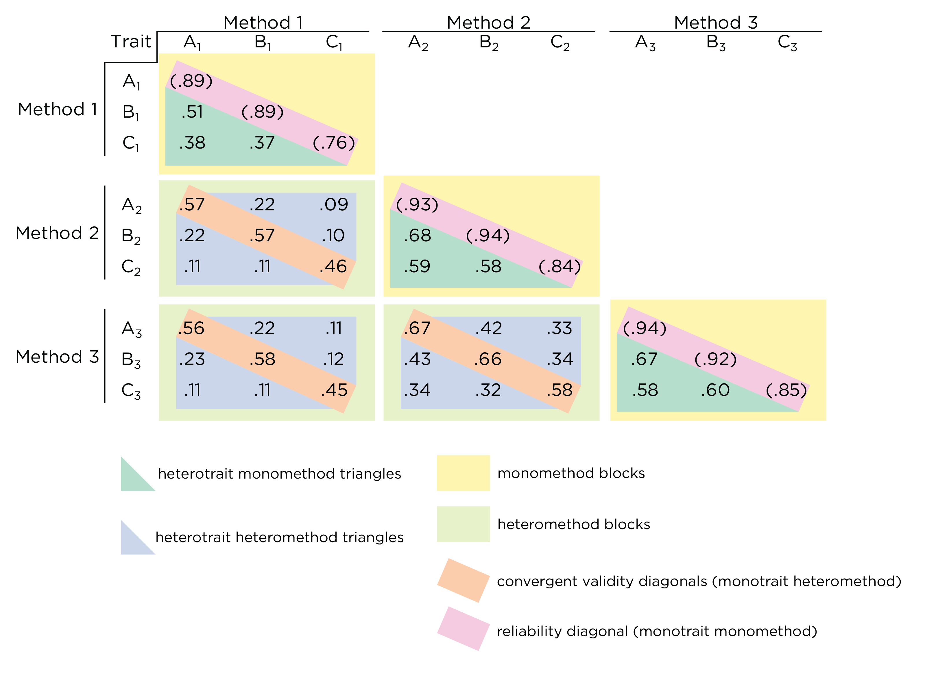
Campbell, D. T., & Fiske, D. W. (1959). Convergent and discriminant validation by the multitrait-multimethod matrix.
Psychological Bulletin,
56(2), 81–105.
https://doi.org/10.1037/h0046016
Clark, L. A., & Watson, D. (2019). Constructing validity: New developments in creating objective measuring instruments.
Psychological Assessment,
31(12), 1412–1427.
https://doi.org/10.1037/pas0000626
Cronbach, L. J., & Meehl, P. E. (1955). Construct validity in psychological tests.
Psychological Bulletin,
52(4), 281–302.
https://doi.org/10.1037/h0040957
Epskamp, S. (2022).
semPlot: Path diagrams and visual analysis of various SEM packages’ output.
https://github.com/SachaEpskamp/semPlot
Exner, J. E. (1974). The Rorschach: A comprehensive system. John Wiley & Sons.
Exner, J. E., & Erdberg, S. P. (2005). The Rorschach, a comprehensive system: Advanced interpretation (3rd ed., Vol. 2). John Wiley & Sons, Inc.
Fiske, D. W., & Campbell, D. T. (1992). Citations do not solve problems.
Psychological Bulletin,
112(3), 393–395.
https://doi.org/10.1037/0033-2909.112.3.393
Fok, C. C. T., & Henry, D. (2015). Increasing the sensitivity of measures to change.
Prevention Science,
16(7), 978–986.
https://doi.org/10.1007/s11121-015-0545-z
Fornell, C., & Larcker, D. F. (1981). Evaluating structural equation models with unobservable variables and measurement error.
Journal of Marketing Research,
18(1), 39–50.
https://doi.org/10.2307/3151312
Furr, R. M. (2017). Psychometrics: An introduction. SAGE publications.
Furr, R. M., & Heuckeroth, S. (2019). The
“quantifying construct validity” procedure: Its role, value, interpretations, and computation.
Assessment,
26(4), 555–566.
https://doi.org/10.1177/1073191118820638
Goodwin, L. D., & Leech, N. L. (2006). Understanding correlation: Factors that affect the size of
r.
The Journal of Experimental Education,
74(3), 249–266.
https://doi.org/10.3200/JEXE.74.3.249-266
Hayes, S. C., Nelson, R. O., & Jarrett, R. B. (1987). The treatment utility of assessment: A functional approach to evaluating assessment quality.
American Psychologist,
42, 963–974.
https://doi.org/10.1037/0003-066X.42.11.963
Henseler, J., Ringle, C. M., & Sarstedt, M. (2015). A new criterion for assessing discriminant validity in variance-based structural equation modeling.
Journal of the Academy of Marketing Science,
43(1), 115–135.
https://doi.org/10.1007/s11747-014-0403-8
Johnson, P. E. (2022).
rockchalk: Regression estimation and presentation.
https://CRAN.R-project.org/package=rockchalk
Leong, F. T. L., & Kalibatseva, Z. (2016). Threats to cultural validity in clinical diagnosis and assessment: Illustrated with the case of Asian Americans. In N. Zane, G. Bernal, & F. T. L. Leong (Eds.), Evidence-based psychological practice with ethnic minorities: Culturally informed research and clinical strategies (pp. 57–74). American Psychological Association.
Marsh, H. W., Guo, J., Lüdtke, O., & Pekrun, R. (2026). Throwing out the bathwater but keeping the baby: Extending
Campbell-Fiske’s multitrait-multimethod framework.
Advances in Methods and Practices in Psychological Science,
9(2), 1–24.
https://doi.org/10.1177/25152459251407652
Meehl, P. E. (1978). Theoretical risks and tabular asterisks:
Sir
Karl,
Sir
Ronald, and the slow progress of soft psychology.
Journal of Consulting and Clinical Psychology,
46(4), 806–834.
https://doi.org/10.1037/0022-006x.46.4.806
Myers, K., & Winters, N. C. (2002). Ten-year review of rating scales.
I:
Overview of scale functioning, psychometric properties, and selection.
Journal of the American Academy of Child & Adolescent Psychiatry,
41(2), 114–122.
https://doi.org/10.1097/00004583-200202000-00004
Nelson-Gray, R. O. (2003). Treatment utility of psychological assessment.
Psychological Assessment,
15(4), 521–531.
https://doi.org/10.1037/1040-3590.15.4.521
Petersen, I. T. (2025).
petersenlab: A collection of R functions by the Petersen Lab.
https://doi.org/10.32614/CRAN.package.petersenlab
Revelle, W. (2024). The seductive beauty of latent variable models: Or why i don’t believe in the
Easter Bunny.
Personality and Individual Differences,
221, 112552.
https://doi.org/10.1016/j.paid.2024.112552
Roemer, E., Schuberth, F., & Henseler, J. (2021). HTMT2–an improved criterion for assessing discriminant validity in structural equation modeling.
Industrial Management & Data Systems,
121(12), 2637–2650.
https://doi.org/10.1108/IMDS-02-2021-0082
Rönkkö, M., & Cho, E. (2020). An updated guideline for assessing discriminant validity.
Organizational Research Methods, 1094428120968614.
https://doi.org/10.1177/1094428120968614
Rosseel, Y., Jorgensen, T. D., & Rockwood, N. (2022).
lavaan: Latent variable analysis.
https://lavaan.ugent.be
Royal, K. (2016).
“Face validity” is not a legitimate type of validity evidence!
The American Journal of Surgery,
212(5), 1026–1027.
https://doi.org/10.1016/j.amjsurg.2016.02.018
Sayal, K., Wyatt, L., Partlett, C., Ewart, C., Bhardwaj, A., Dubicka, B., Marshall, T., Gledhill, J., Lang, A., Sprange, K., Thomson, L., Moody, S., Holt, G., Bould, H., Upton, C., Keane, M., Cox, E., James, M., & Montgomery, A. (2025). The clinical and cost effectiveness of a
STAndardised DIagnostic Assessment for children and adolescents with emotional difficulties: The
STADIA multi-centre randomised controlled trial.
Journal of Child Psychology and Psychiatry,
66(6), 805–820.
https://doi.org/10.1111/jcpp.14090
Schmidt, F. L., & Hunter, J. E. (1996). Measurement error in psychological research: Lessons from 26 research scenarios.
Psychological Methods,
1(2), 199–223.
https://doi.org/10.1037/1082-989X.1.2.199
Schneider, W. J. (2021).
simstandard: Generate standardized data.
https://github.com/wjschne/simstandard
Sechrest, L. (1963). Incremental validity: A recommendation.
Educational and Psychological Measurement,
23, 153–158.
https://doi.org/10.1177/001316446302300113
Shadish, W. R., Cook, T. D., & Campbell, D. T. (2002). Experimental and quasi-experimental designs for generalized causal inference. Houghton Mifflin.
Silver, N. (2012). The signal and the noise: Why so many predictions fail–but some don’t. Penguin.
Slack, M. K., & Draugalis, J., Jolaine R. (2001). Establishing the internal and external validity of experimental studies.
American Journal of Health-System Pharmacy,
58(22), 2173–2181.
https://doi.org/10.1093/ajhp/58.22.2173
Stallworthy, I. C., DeJoseph, M. L., Heuvel, M. I. van den, Berry, D., & Frankenhuis, W. E. (in press). Developmental frameworks, what have you done for me lately?
Development and Psychopathology.
https://doi.org/10.1017/S0954579425101016
Voorhees, C. M., Brady, M. K., Calantone, R., & Ramirez, E. (2016). Discriminant validity testing in marketing: An analysis, causes for concern, and proposed remedies.
Journal of the Academy of Marketing Science,
44(1), 119–134.
https://doi.org/10.1007/s11747-015-0455-4
Wood, J. M., Nezworski, M. T., Garb, H. N., & Lilienfeld, S. O. (2001). Problems with the norms of the
Comprehensive System for the
Rorschach: Methodological and conceptual considerations.
Clinical Psychology: Science and Practice,
8(3), 397–402.
https://doi.org/10.1093/clipsy.8.3.397
Wood, J. M., Teresa, P. M., Garb, H. N., & Lilienfeld, S. O. (2001). The misperception of psychopathology: Problems with the norms of the
Comprehensive System for the
Rorschach.
Clinical Psychology: Science and Practice,
8(3), 350–373.
https://doi.org/10.1093/clipsy.8.3.350


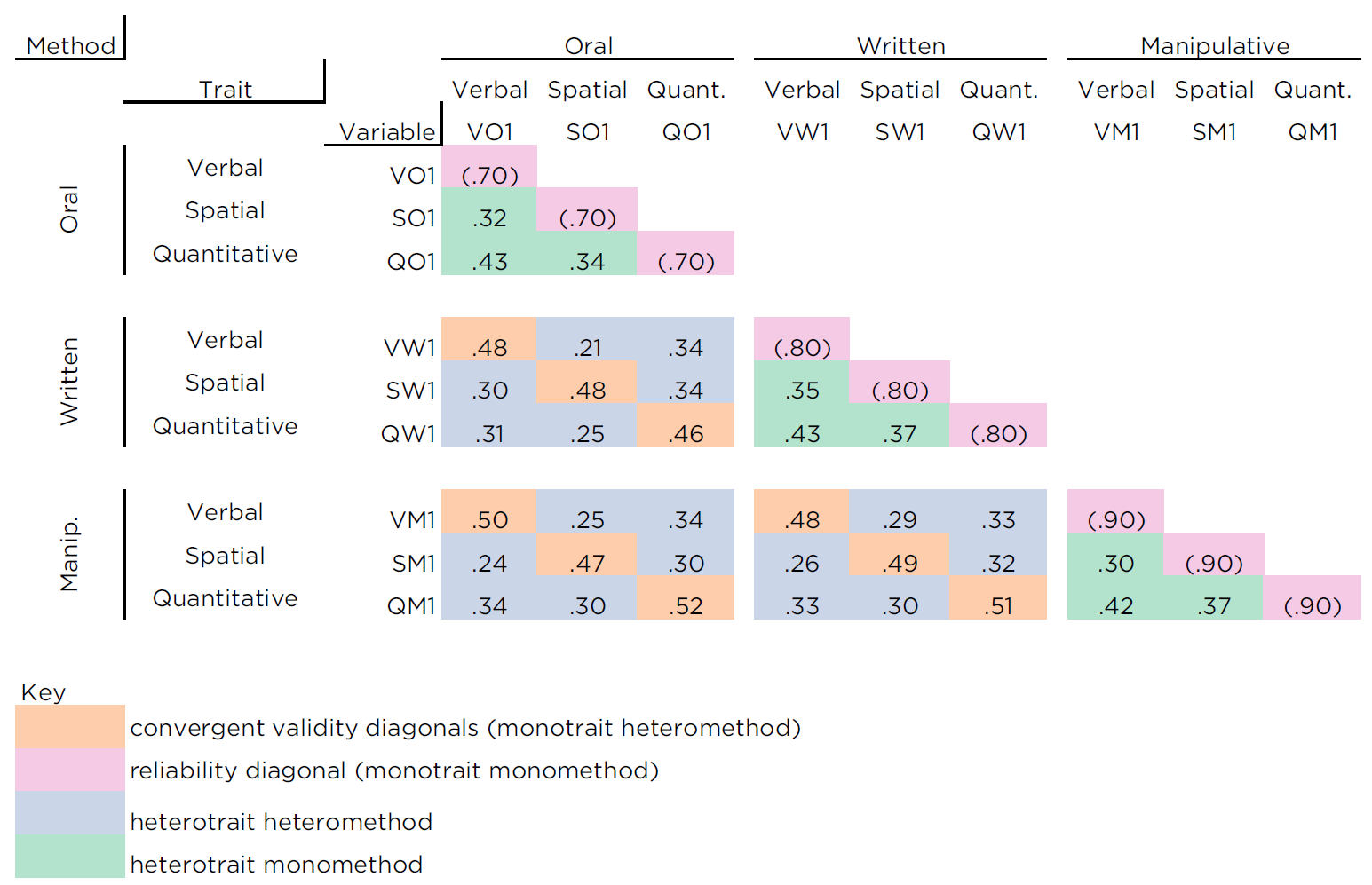
![Multitrait-Multimethod Matrix. (Figure reprinted from Campbell and Fiske [-@Campbell1959], Table 1, p. 82. Campbell, D. T., & Fiske, D. W. (1959). Convergent and discriminant validation by the multitrait-multimethod matrix. *Psychological Bulletin*, *56*, 81–105. <https://doi.org/10.1037/h0046016>)](images/campbellFiske.png)