I want your feedback to make the book better for you and other readers. If you find typos, errors, or places where the text may be improved, please let me know. The best ways to provide feedback are by GitHub or hypothes.is annotations.
Opening an issue or submitting a pull request on GitHub: https://github.com/isaactpetersen/Principles-Psychological-Assessment
Adding an annotation using hypothes.is.
To add an annotation, select some text and then click the
symbol on the pop-up menu.
To see the annotations of others, click the
symbol in the upper right-hand corner of the page.
Chapter 16 Test Bias
16.1 Overview of Bias
There are multiple definitions of the term “bias” depending on the context. In general, bias is a systematic error (Reynolds & Suzuki, 2012). Mean error is an example of systematic error, and is sometimes called bias. Cognitive biases are systematic errors in thinking, including confirmation bias and hindsight bias. Method biases are a form of systematic error that involve the influence of measurement on a person’s score that is not due to the person’s level on the construct. Method biases include response biases or response styles, including acquiescence and social desirability bias. Attentional bias refers to the tendency to process some types of stimuli more than others.
Sometimes bias is used to refer in particular to systematic error (in measurement, prediction, etc.) as a function of group membership, where test bias refers to the same score having different meaning for different groups. Under this meaning, a test is unbiased if a given test score has the same meaning regardless of group membership. For example, a test is biased if there is differential validity of test scores for groups (e.g., age, education, culture, race, sex). Test bias would exist, for instance, if a test is a less valid predictor for racial minorities or linguistic minorities. Test bias would also exist if scores on the Scholastic Aptitude Test (SAT) under-estimate women’s grades in college, for instance.
There are some known instances of test bias, as described in Section 16.3. Research has not produced much empirical evidence of test bias (Brown et al., 1999; Hall et al., 1999; Jensen, 1980; Kuncel & Hezlett, 2010; Reynolds et al., 2021; Reynolds & Suzuki, 2012; Sackett et al., 2008; Sackett & Wilk, 1994), though some item-level bias is not uncommon. Moreover, where test bias has been observed, it is often small, unclear, and does not always generalize (N. S. Cole, 1981). However, just because there is not much empirical evidence of test bias does not mean that test bias does not exist. Moreover, just because a test does not show bias does not mean that it should be used. Furthermore, just because a test does not show bias does not mean that there are not race-, social class-, and gender-related biases in clinical judgment during the assessment process.
It is also worth pointing out that group differences in scores do not necessarily indicate bias. Group differences in scores could reflect true group differences in the construct. For instance, women have better verbal abilities, on average, compared to men. So, if women’s scores on a verbal ability test are higher on average than men’s scores, this would not be sufficient evidence for bias.
There are two broad categories of test bias:
Predictive bias refers to differences between groups in the relation between the test and criterion. As with all criterion-related validity tests, the findings depend on the strength and quality of the criterion. Test structure bias refers to differences in the internal test characteristics across groups.
16.2 Ways to Investigate/Detect Test Bias
16.2.1 Predictive Bias
Predictive bias exists when differences emerge between groups in terms of predictive validity to a criterion. It is assessed by using a regression line looking at the association between test score and job performance. For instance, consider a 2x2 confusion matrix used for the standard prediction problem. A confusion matrix for whom to select for a job is depicted in Figure 16.1.
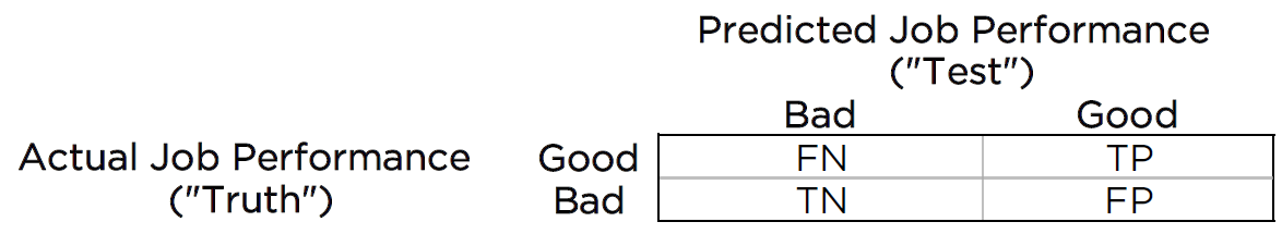
Figure 16.1: 2x2 Confusion Matrix for Job Selection. TP = true positive; TN = true negative; FP = false positive; FN = false negative.
We can also visualize the confusion matrix in terms of a scatterplot of the test scores (i.e., predicted job performance) and the “truth” scores (i.e., actual job performance), as depicted in Figure 16.2. The predictor (test score) is on the x-axis. The criterion (job performance) is on the y-axis. The quadrants reflect the cutoffs (i.e., thresholds) imposed from the 2x2 confusion matrix. The vertical line reflects the cutoff for selecting someone for a job. The horizontal line reflects the cutoff for good job performance (i.e., people who should have been selected for the job).
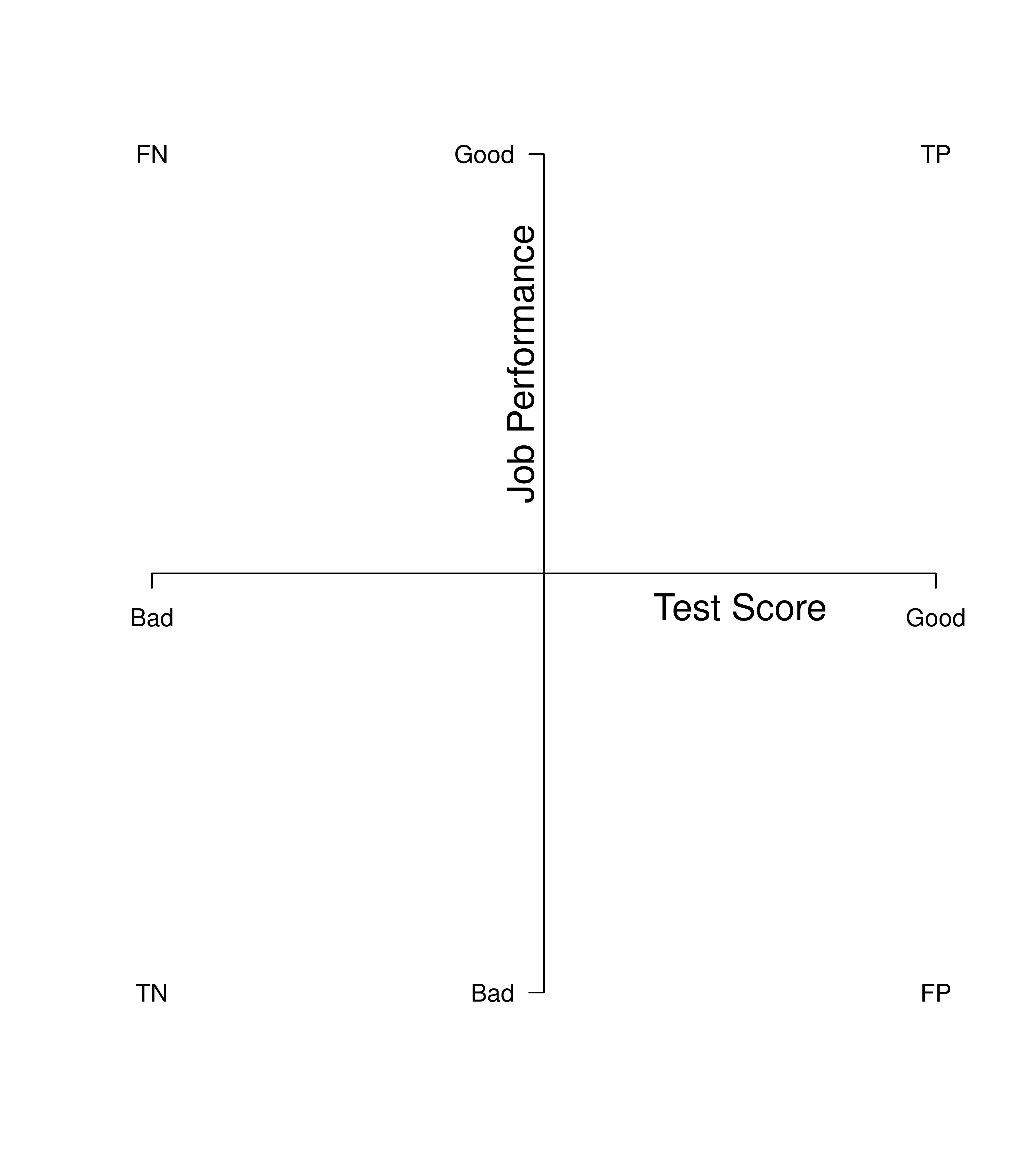
Figure 16.2: 2x2 Confusion Matrix for Job Selection in the Form of a Graph With Predicted Performance on the x-Axis and Actual Job Performance on the y-Axis. TP = true positive; TN = true negative; FP = false positive; FN = false negative.
The data points in the top right quadrant are true positives: people who the test predicted would do a good job and who did a good job. The data points in the bottom left quadrant are true negatives: people who the test predicted would do a poor job and who would have done a poor job. The data points in the bottom right quadrant are false positives: people who the test predicted would do a good job and who did a poor job. The data points in the top left quadrant are false negatives: people who the test predicted would do a poor job and who would have done a good job.
Figure 16.3 depicts a strong predictor. The best-fit regression line has a steep slope where there are lots of data points that are true positives and true negatives, with relatively few false positives and false negatives.
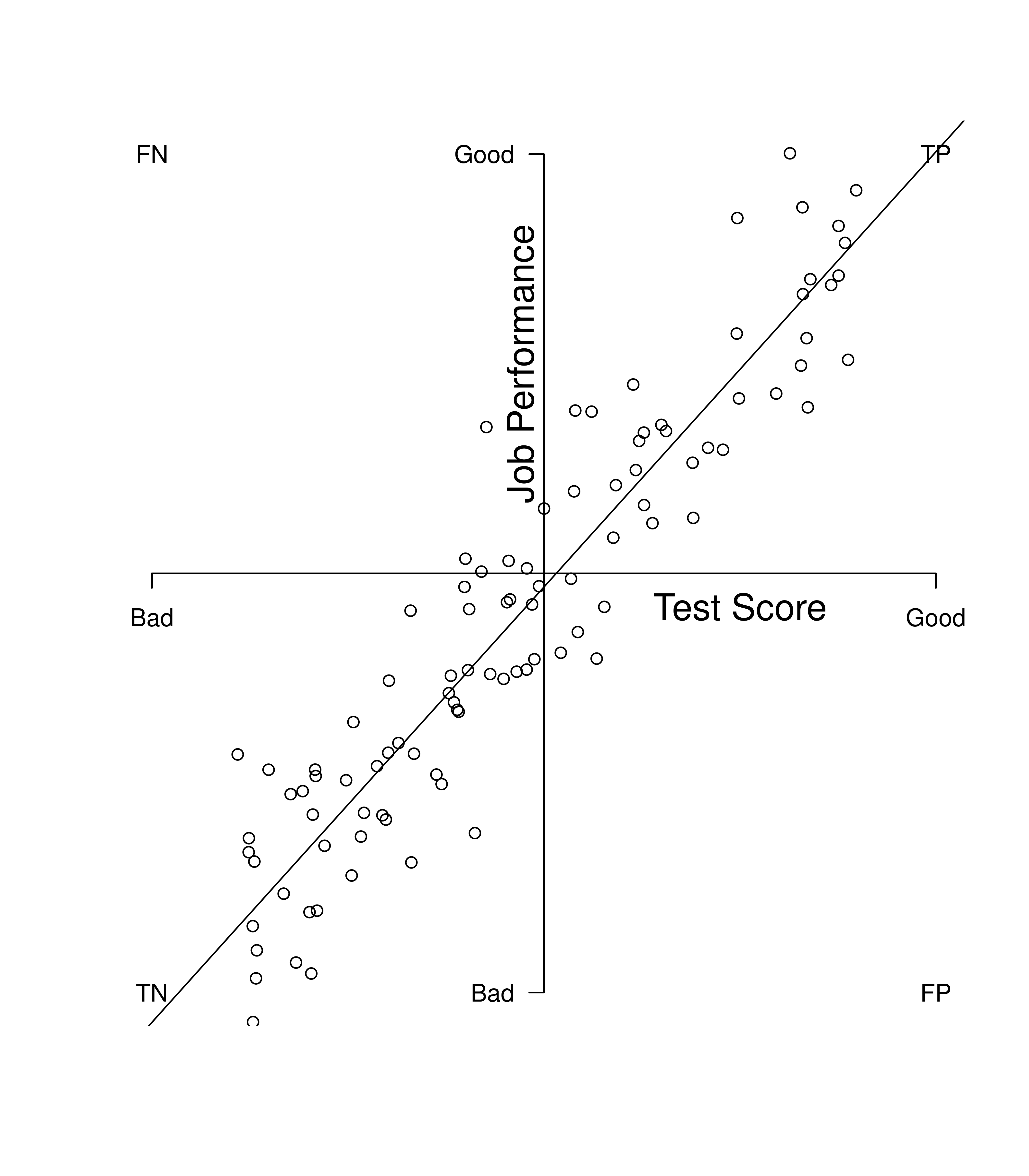
Figure 16.3: Example of a Strong Predictor. TP = true positive; TN = true negative; FP = false positive; FN = false negative.
Figure 16.4 depicts a poor predictor. The best-fit regression line has a shallow slope where there are just as many data points that are in the false cells (false positives and false negatives) as there are in the true cells (true positives and true negatives). In general, the steeper the slope, the better the predictor.
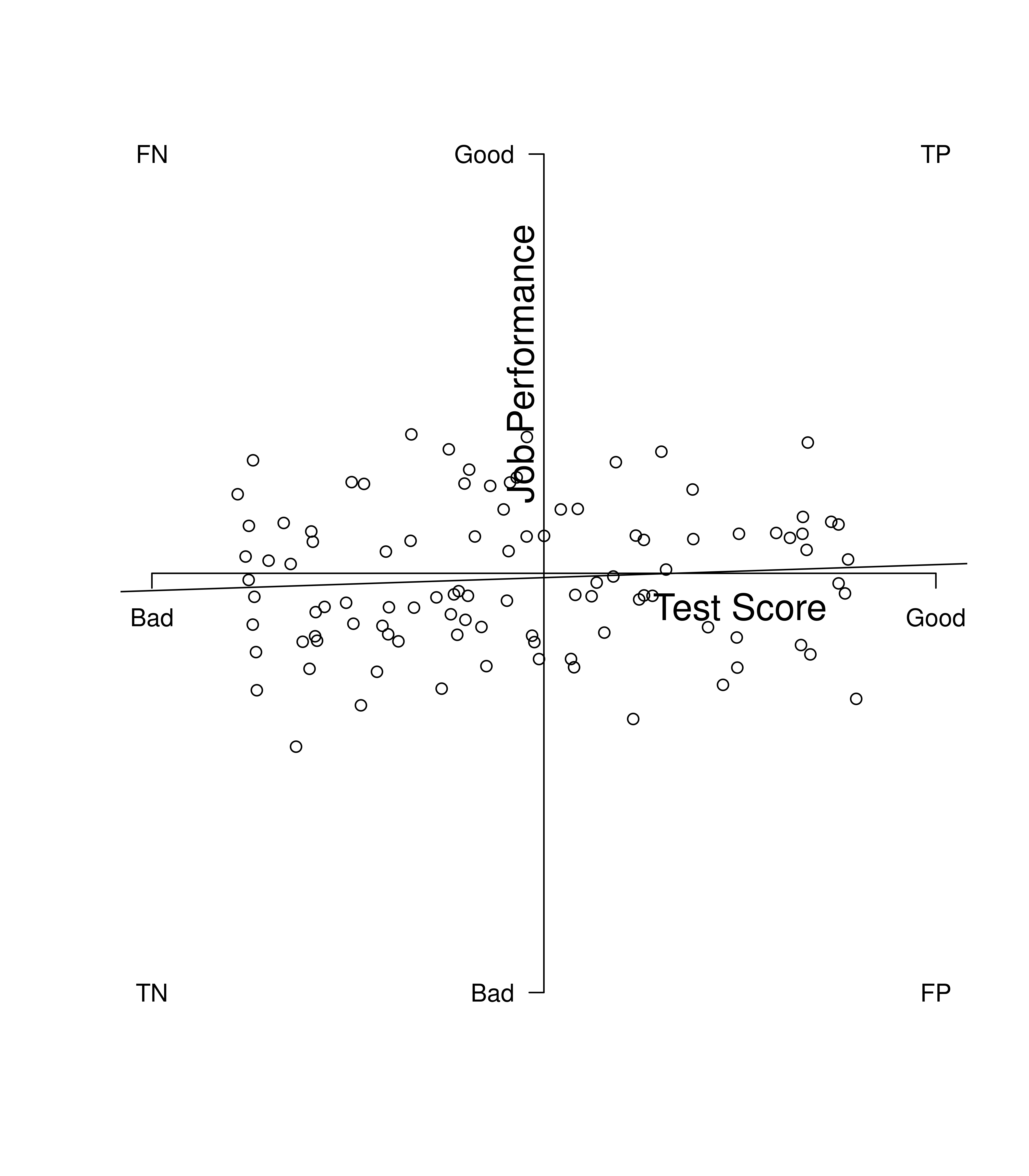
Figure 16.4: Example of a Poor Predictor. TP = true positive; TN = true negative; FP = false positive; FN = false negative.
We can evaluate predictive bias using a best-fit regression line between the predictor and criterion for each group.
16.2.1.1 Types of Predictive Bias
There are three types of predictive bias:
The slope of the regression line is the steepness of the line. The intercept of the regression line is the y-value of the point where the line crosses the y-axis (i.e., when \(x = 0\)). If a measure shows predictive test bias, when looking at the regression line for each group, the groups’ regression lines differ in either slopes and/or intercepts.
16.2.1.1.1 Different Slopes
Predictive bias in terms of different slopes exists when there are differences in the slope of the regression line between minority and majority groups. The slope describes the direction and steepness of the regression line. The slope of a regression line is the amount of change in \(y\) for every unit change in \(x\) (i.e., rise over run). Differing slopes indicate differential predictive validity, in which the test is a more effective predictor of performance in one group over the other. Different slopes predictive bias is depicted in Figure 16.5. In the figure, the predictor performs well in the majority group. However, the slope is close to zero in the minority group, indicating that there is no association between the predictor and the criterion for the minority group.
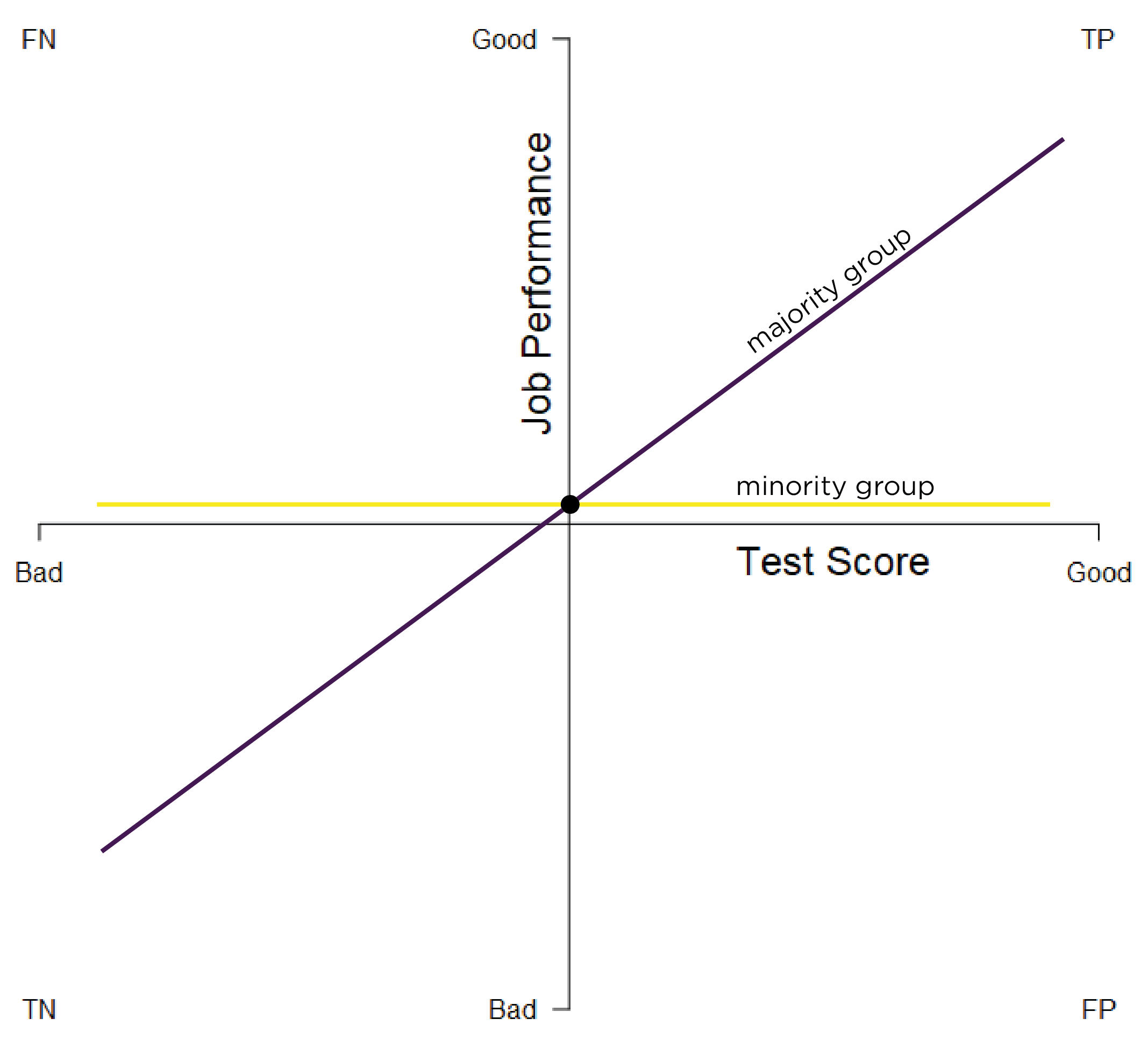
Figure 16.5: Test Bias: Different Slopes. TP = true positive; TN = true negative; FP = false positive; FN = false negative.
Different slopes can especially occur if we develop our measure and criterion based on the normative majority group. Not much evidence has found empirical evidence of different slopes across groups. However, samples often do not have the power to detect differing slopes (Aguinis et al., 2010). Theoretically, to fix biases related to different slopes, you should find another measure that is more predictive for the minority group. If the predictor is a strong predictor in both groups but shows slight differences in the slope, within-group norming could be used.
16.2.1.1.2 Different Intercepts
Predictive bias in terms of different intercepts exists when there are differences in the intercept of the regression line between minority and majority groups. The \(y\)-intercept describes the point on the \(y\)-axis that the line intersects with the \(y\)-axis (when \(x = 0\)). When the distributions have similar slopes, intercept differences suggest that the measure systematically under- or over-estimates group performance relative to the person’s ability. The same test score leads to systematically different predictions for the majority and minority groups. In other words, minority group members get different tests scores than majority group members with the same ability. Different intercepts predictive bias is depicted in Figure 16.6.
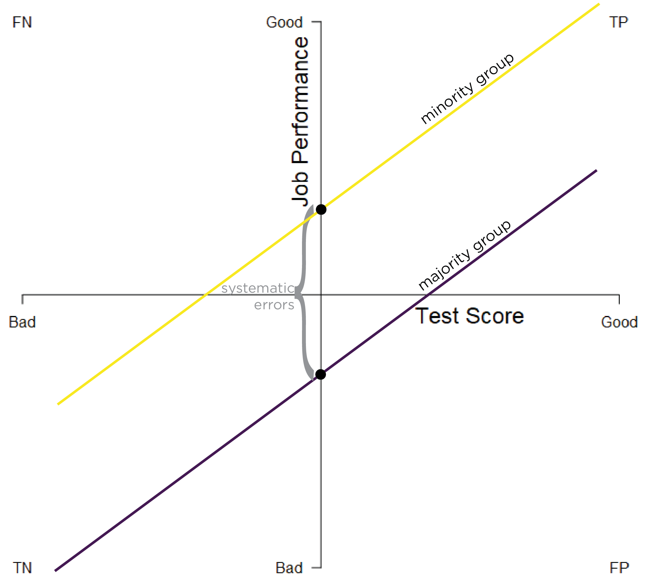
Figure 16.6: Test Bias: Different Intercepts. TP = true positive; TN = true negative; FP = false positive; FN = false negative.
A higher intercept (relative to zero) indicates that the measure under-estimates a person’s ability (at that test score)—i.e., the person’s job performance is better than what the test score would suggest. A lower intercept (relative to zero) indicates that the measure over-estimates a person’s ability (at that test score)—i.e., the person’s job performance is worse than what the test score would suggest. Figure 16.6 indicates that the measure systematically under-estimates the job performance of the minority group.
Performance among members of a minority group could be under- or over-estimated. For example, historically, women’s grades in math and engineering classes tended to be under-estimated by the Scholastic Aptitude Test [SAT; M. J. Clark & Grandy (1984)]. However, where intercept differences have been observed, measures often show small over-estimation of school and job performance among minority groups (Reynolds & Suzuki, 2012). For example, women’s physical strength and endurance is over-estimated based on physical ability tests (Sackett & Wilk, 1994). In addition, over-estimation of African Americans’ and Hispanics’ school and job performance has been observed based on cognitive ability tests (N. S. Cole, 1981; Reynolds & Suzuki, 2012; Sackett et al., 2008; Sackett & Wilk, 1994). At the same time, the Black–White difference in job performance is less than the Black–White difference in test performance.
The over-prediction of lower-scoring groups is likely mostly an artifact of measurement error (L. S. Gottfredson, 1994). The over-estimation of African Americans’ and Hispanics’ school and job performance may be due to measurement error in the tests. Moreover, test scores explain only a portion of the variation in job performance. Black people are far less disadvantaged on the noncognitive determinants of job performance than on the cognitive ones. Nevertheless, the over-estimation that has been often observed is on average—the performance is not over-estimated for all individuals of the groups even if there is an average over-estimation effect. In addition, simulation findings indicate that lower intercepts (i.e., over-estimation) among minority groups compared to majority groups could be observed if there are different slopes but not different intercepts in the population, because different slopes are likely to go undetected due to low power (Aguinis et al., 2010). That is, if a test shows weaker validity for a minority group than the majority group, it could appear as different intercepts that favor the minority group when, in fact, it reflects shallower slopes of the minority group that go undetected.
Predictive biases in intercepts could especially occur if we develop tests that are based on the majority group, and the items assess constructs other than the construct of interest which are systematically biased in favor of the majority group or against the minority group. Arguments about reduced power to detect differences are less relevant for intercepts and means than for slopes.
To correct for a bias in intercepts, we could add bonus points to the scores for the minority group to correct for the amount of the systematic error, and to result in the same regression line. But if the minority group is over-predicted (as has often been the case where intercept differences have been observed), we would not want to use score adjustment to lower the minority group’s scores.
16.2.1.1.3 Different Intercepts and Slopes
Predictive bias in terms of different intercepts and slopes exists when there are differences in the intercept and slope of the regression line between minority and majority groups. In cases of different intercepts and slopes, there is both differential validity (because the regression lines have different slopes), as well as varying under- and over-estimation of groups’ performance at particular scores. Different intercepts and slopes predictive bias is depicted in Figure 16.7.
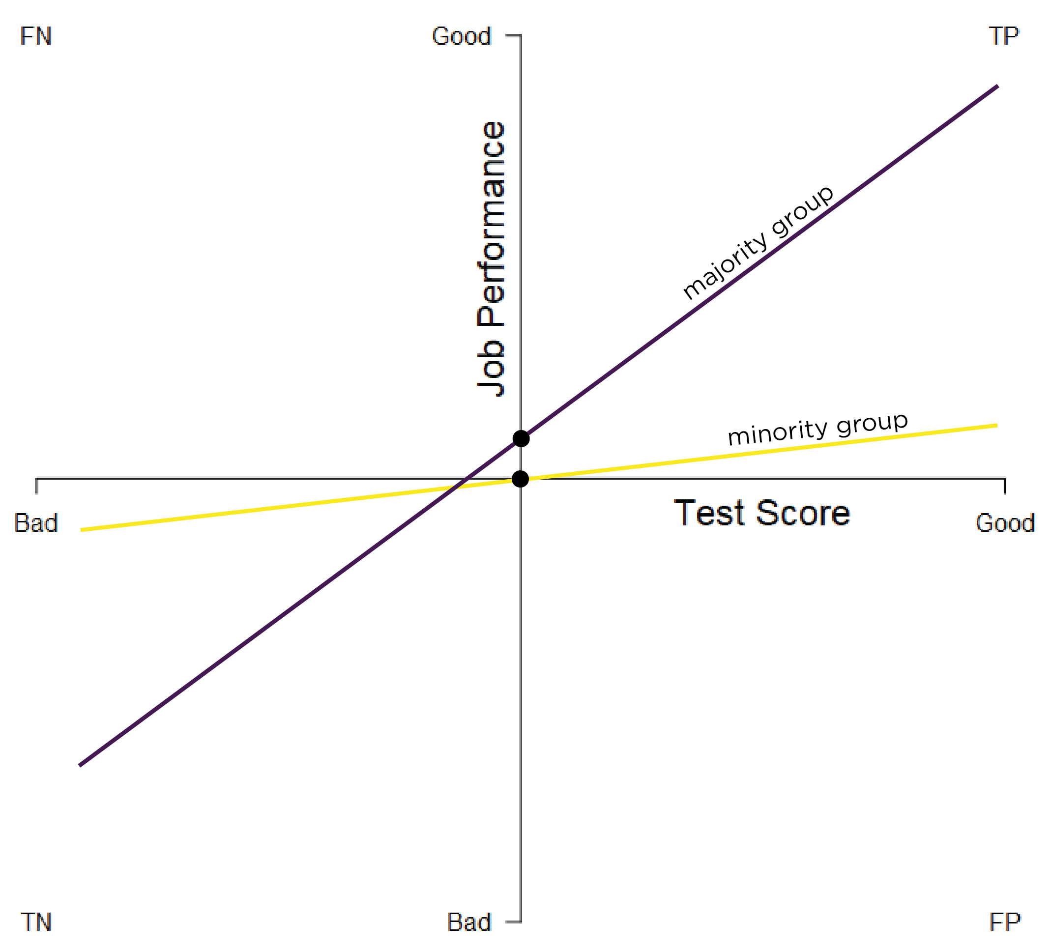
Figure 16.7: Test Bias: Different Intercepts and Slopes. TP = true positive; TN = true negative; FP = false positive; FN = false negative.
In instances of different intercepts and slopes predictive bias, a measure can simultaneously over-estimate and under-estimate a person’s ability at different test scores. For instance, a measure can under-estimate a person’s ability at higher test scores and can over-estimate a person’s ability at lower test scores.
Different intercepts and slopes across groups is possibly more realistic than just different intercepts or just different slopes. However, different intercepts and slopes predictive bias is more complicated to study, represent, and resolve. It is difficult to examine because of complexity, and it is not easy to fix. Currently, we have nothing to address different intercepts and slopes predictive bias. We would need to use a different measure or measures for each group.
16.2.2 Test Structure Bias
In addition to predictive bias, another type of test bias is test structure bias. Test structure bias involves differences in internal test characteristics across groups. Examining test structure bias is different from examining the total score, as is used when examining predictive bias. Test structure bias can be identified empirically or based on theory/judgment.
Empirically, test structure bias can be examined in multiple ways.
16.2.2.1 Empirical Approaches to Identification
16.2.2.1.1 Item \(\times\) Group tests (ANOVA)
Item \(\times\) Group tests in analysis of variance (ANOVA) examine whether the difference between groups on the overall score match comparisons among smaller items sets between groups. Item \(\times\) Group tests are used to rule out that items are operating in different ways in different groups. If the items operate in different ways in different groups, they do not have the same meaning across groups. For example, if we are going to use a measure for multiple groups, we would expect its items to operate similarly across groups. So, if women show higher scores on a depression measure compared to men, would also expect them to show similar elevations on each item (e.g., sleep loss).
16.2.2.1.2 Item Response Theory
Using item response theory, we can examine differential item functioning (DIF). Evidence of DIF, indicates that there are differences between group in terms of discrimination and/or difficulty/severity of items. Differences between groups in terms of the item characteristic curve (which combines the item’s discrimination and severity) would be evidence against construct validity invariance between the groups and would provide evidence of bias. DIF examines stretching and compression of different groups. As an example, consider the item “bites others” in relation to externalizing problems. The item would be expected to show a weaker discrimination and higher severity in adults compared to children. DIF is discussed in Section 16.9.
16.2.2.1.3 Confirmatory Factor Analysis
Confirmatory factor analysis allows tests of measurement invariance (also called factorial invariance). Measurement invariance examines whether the factor structure of the underlying latent variables in the test is consistent across groups. It also examines whether the manifestation of the construct differs between groups. Measurement invariance is discussed in Section 16.10.
Even if you find the same slope and intercepts across groups in a prediction model, the measure would still be assessing different constructs across groups if the measure has a different factor structure between the groups. A different factor structure across groups is depicted in Figure 16.8.
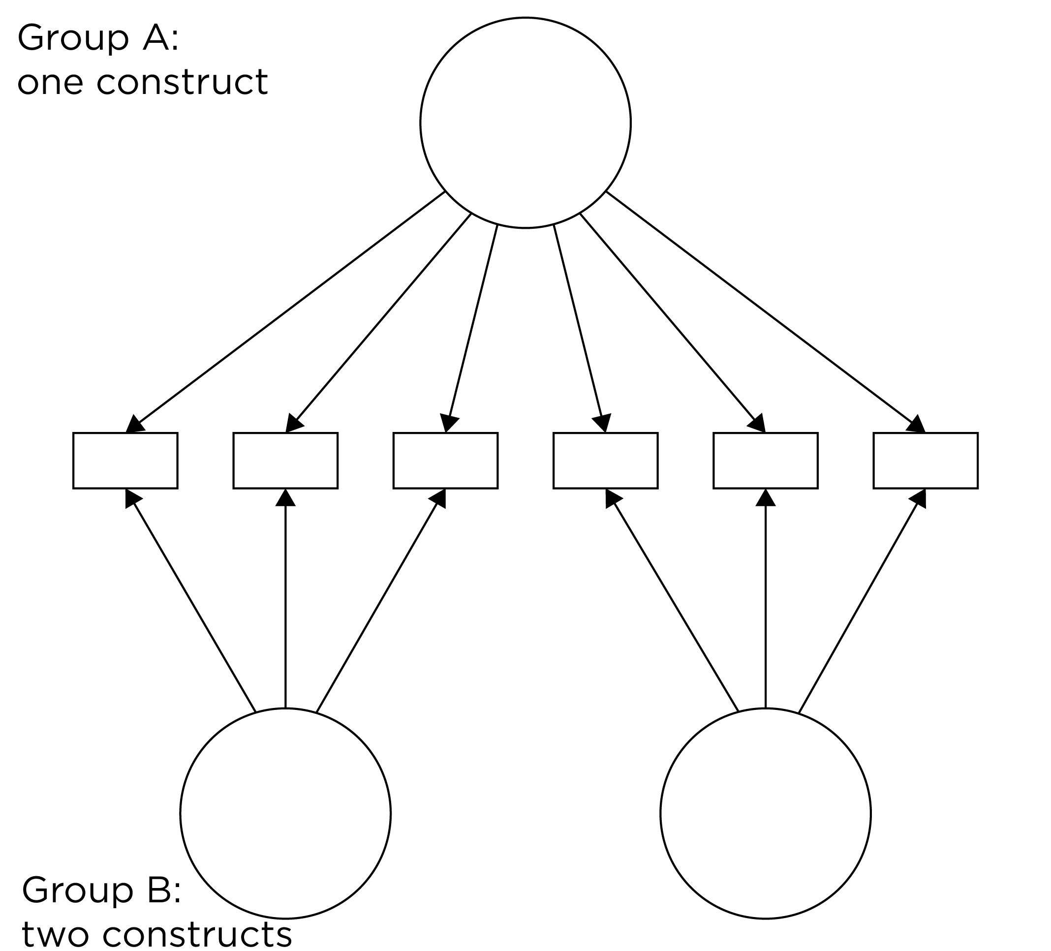
Figure 16.8: Different Factor Structure Across Groups.
An example of a different factor structure across groups is the differentiation of executive functions from two factors to three factors (inhibition, working memory, cognitive flexibility) across childhood (K. Lee et al., 2013).
There are different degrees of measurement invariance (for a review, see Putnick & Bornstein, 2016):
- Configural invariance: same number of factors in each group, and which indicators load on which factors are the same in each group (i.e., the same pattern of significant loadings in each group).
- Metric (“weak factorial”) invariance: items have the same factor loadings (discrimination) in each group.
- Scalar (“strong factorial”) invariance: items have the same intercepts (difficulty/severity) in each group.
- Residual (“strict factorial”) invariance: items have the same residual/unique variances in each group.
16.2.2.1.4 Structural Equation Modeling
Structural equation modeling is a confirmatory factor analysis (CFA) model that incorporates prediction. Structural equation modeling allows examining differences in the underlying structure with differences in prediction in the same model.
16.2.2.1.5 Signal Detection Theory
Signal detection theory is a dynamic measure of bias. It allows examining the overall bias in selection systems, including both accuracy and errors at various cutoffs (sensitivity, specificity, positive predictive value, and negative predictive value), as well as accuracy across all possible cutoffs (the area under the receiver operating characteristic curve). While there may be similar predictive validity between groups, the type of errors we are making across groups might differ. It is important to decide which types of error to emphasize depending on the fairness goals and examining sensitivity/specificity to adjust cutoffs.
16.2.2.1.6 Empirical Evidence of Test Structure Bias
It is not uncommon to find items that show differences across groups in severity (intercepts) and/or discrimination (factor loadings). However, cross-group differences in item functioning tend to be small and not consistent across studies, suggesting that some of the differences may reflect Type I errors that result from sampling error and multiple testing. That said, some instances of cross-group differences in item parameters could reflect test structure bias that is real and important to address.
16.2.2.2 Theoretical/Judgmental Approaches to Identification
16.2.2.2.1 Facial Validity Bias
Facial validity bias considers the extent to which an average person thinks that an item is biased—i.e., the item has differing validity between minority and majority groups. If so, the item should be reconsidered. Does an item disfavor certain groups? Is the language specific to a particular group? Is it offensive to some people? This type of judgment moves into the realm of whether or not an item should be used.
16.2.2.2.2 Content Validity Bias
Content validity bias is determined by judgments of construct experts who look for items that do not do an adequate job assessing the construct between groups. A construct may include some content facets in one group, but may include different content facets in another group, as depicted in Figure 16.9.

Figure 16.9: Different Content Facets in a Given Construct for Two Groups.
Examples include information questions and vocabulary questions on the Wechsler Adult Intelligence Scale. If an item is linguistically complicated, grammatically complex or convoluted, or a double negative, it may be less valid or predictive for rural populations and those with less education.
Also, stereotype threat may contribute to content validity bias. Stereotype threat occurs when people are or feel at risk of conforming themselves to stereotypes about their social group, thus leading them to show poorer performance in ways that are consistent with the stereotype. Stereotype threat may partially explain why some women may perform more poorly on some math items than some men.
Another example of content validity bias is when the same measure is used to assess a construct across ages even though the construct shows heterotypic continuity. Heterotypic continuity occurs when a construct changes in its behavioral manifestation with development (Petersen et al., 2020). That is, the same construct may look different at different points in development. An example of a construct that shows heterotypic continuity is externalizing problems. In early childhood, externalizing problems often manifest in overt forms, including physical aggression (e.g., biting) and temper tantrums. By contrast, in adolescence and adulthood, externalizing problems more often manifest in covert ways, including relational aggression and substance use. Content validity and facial validity bias judgments are often related, but not always.
16.3 Examples of Bias
As described in the overview in Section 16.1, there is not much empirical evidence of test bias (Brown et al., 1999; Hall et al., 1999; Jensen, 1980; Kuncel & Hezlett, 2010; Reynolds et al., 2021; Reynolds & Suzuki, 2012; Sackett et al., 2008; Sackett & Wilk, 1994). That said, some item-level bias is not uncommon. One instance of test bias is that, historically, women’s grades in math and engineering classes tended to be under-estimated by the Scholastic Aptitude Test [SAT; M. J. Clark & Grandy (1984)]. Fernández & Abe (2018) review the evidence on other instances of test and item bias. For instance, test bias can occur if a subgroup is less familiar with the language, the stimulus material, or the response procedures, or if they have different response styles. In addition to test bias, there are known patterns of bias in clinical judgment, as described in Section 25.3.11.
16.4 Test Fairness
There is interest in examining more than just the accuracy of measures. It is also important to examine the errors being made and differentiate the weight or value of different kinds of errors (and correct decisions). Consider an example of an unbiased test, as depicted in Figure 16.10, adapted from L. S. Gottfredson (1994). Although the example is of a White group and a Black group, we could substitute any two groups into the example (e.g., males versus females).
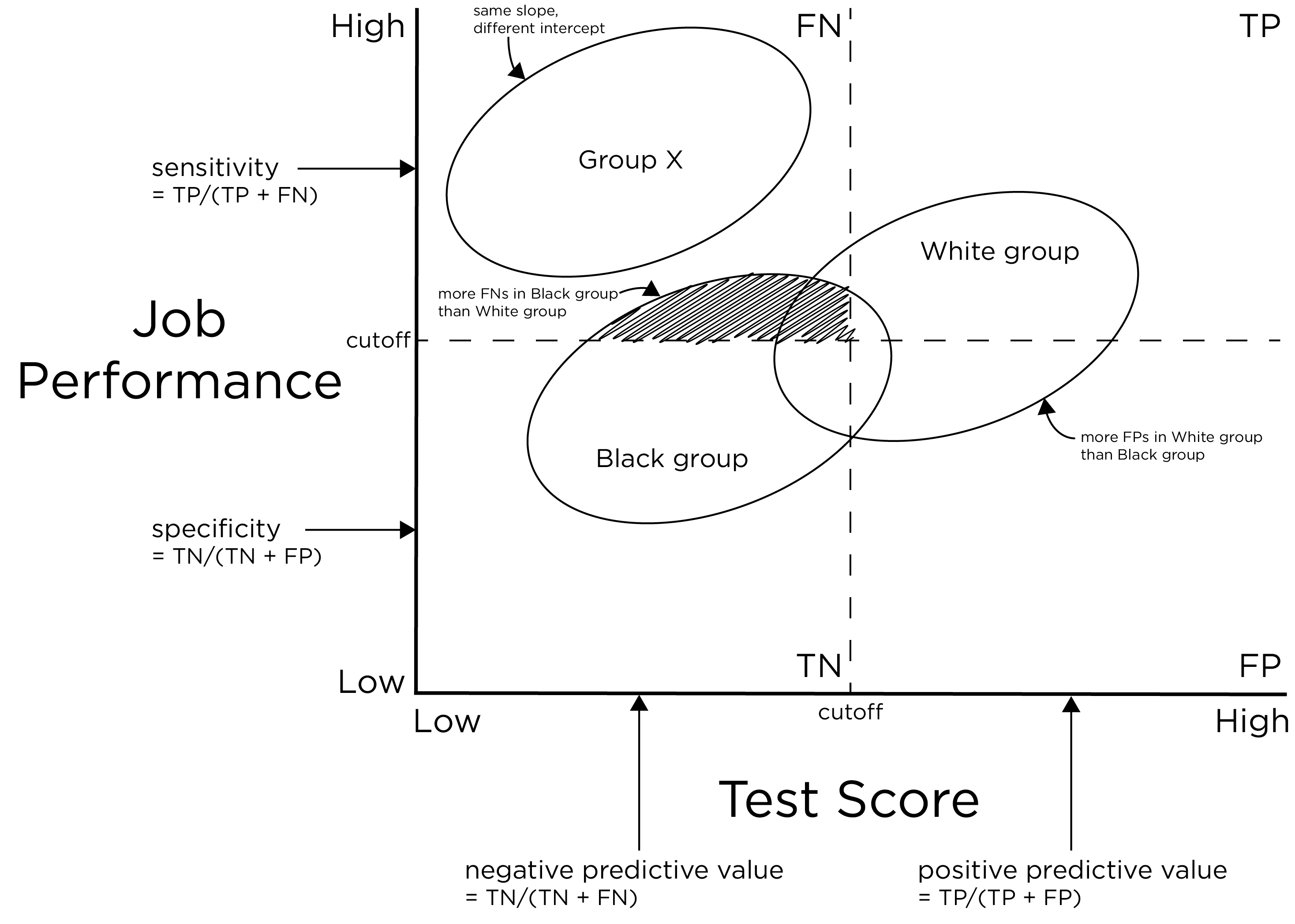
Figure 16.10: Potential Unfairness in Testing. The ovals represent the distributions of individuals’ performance both on a test and a job performance criterion. TP = true positive; TN = true negative; FP = false positive; FN = false negative. (Adapted from L. S. Gottfredson (1994), Figure 1, p. 958. Gottfredson, L. S. (1994). The science and politics of race-norming. American Psychologist, 49(11), 955–963. https://doi.org/10.1037/0003-066X.49.11.955)
The example is of an unbiased test between White and Black job applicants. There are no differences between the two groups in terms of slope. If we drew a regression line, the line would go through the centroid of both ovals. Thus, the measure is equally predictive in both groups even though that the Black group failed the test at a higher rate than the White group. Moreover, there is no difference between the groups in terms of intercept. Thus, the performance of one group is not over-estimated relative to the performance of the other group. To demonstrate what a different intercept would look like, Group X shows a different intercept. In sum, there is no predictive validity bias between the two groups. But just because the test predicts just as well in both groups does not mean that the selection procedures are fair.
Although the test is unbiased, there are differences in the quality of prediction: there are more false negatives in the Black group compared to the White group. This gives the White group an advantage and the Black group additional disadvantages. If the measure showed the same quality of prediction, we would say the test is fair. The point of the example is that just because a test is unbiased does not mean that the test is fair.
There are two kinds of errors: false negatives and false positives. Each error type has very different implications. False negatives would be when the test predicts that an applicant would perform poorly and we do not give them the job even though they would have performed well. False negatives have a negative effect on the applicant. And, in this example, there are more false negatives in the Black group. By contrast, false positives would be when we predict that an applicant would do well, and we give them the job but they perform poorly. False positives are a benefit to the applicant but have a negative effect on the employer. In this example, there are more false positives in the White group, which is an undeserved benefit based on the selection ratio; therefore, the White group benefits.
In sum, equal accuracy of prediction (i.e., equal total number of errors) does not necessarily mean the test is fair; we must examine the types of errors. Merely ensuring accuracy does not ensure fairness!
16.4.1 Adverse Impact
Adverse impact is defined as rejecting members of one group at a higher rate than another group. Adverse impact is different from test validity. According to federal guidelines, adverse impact is present if the selection rate of one group is less than four-fifths (80%) the selection rate of the group with the highest selection rate.
There is much more evidence of adverse impact than test bias. Indeed, disparate impact of tests on personnel selection across groups is the norm rather than the exception, even when using valid tests that are unbiased, which in part reflect group-related differences in job-related skills (L. S. Gottfredson, 1994). Examples of adverse impact include:
- physical ability tests, which produce substantial adverse impact against women (despite over-estimation of women’s performance),
- cognitive ability tests, which produce substantial impact against some ethnic minority groups, especially Black and Hispanic people (despite over-estimation of Black and Hispanic people’s performance), even though cognitive ability tests tend to be among the strongest predictors of job performance (Sackett et al., 2008; Schmidt & Hunter, 1981), and
- personality tests, which produce higher estimates of dominance among men than women; it is unclear whether this has predictive bias.
16.4.2 Bias Versus Fairness
Whether a measure is accurate or shows test bias is a scientific question. By contrast, whether a test is fair and thus should be used for a given purpose is not just a scientific question; it is also an ethical question. It involves the consideration of the potential consequences of testing in terms of social values and consequential validity.
16.4.3 Operationalizing Fairness
There are many perspectives to what should be considered when evaluating test fairness (American Educational Research Association et al., 2014; Camilli, 2013; Committee on the General Aptitude Test Battery et al., 1989; Dorans, 2017; Fletcher et al., 2021; Gipps & Stobart, 2009; Helms, 2006; Jonson & Geisinger, 2022; Melikyan et al., 2019; Sackett et al., 2008; Thorndike, 1971; Zieky, 2006, 2013). As described in Fletcher et al. (2021), there are three primary ways of operationalizing fairness:
- Equal outcomes: the selection rate is the same across groups.
- Equal opportunity: the sensitivity (true positive rate; 1 \(-\) false negative rate) is the same across groups.
- Equal odds: the sensitivity is the same across groups and the specificity (true negative rate; 1 \(-\) false positive rate) is the same across groups.
For example, the job selection procedure shows equal outcomes if the proportion of men selected is equal to the proportion of women selected. The job selection procedure shows equal opportunity if, among those who show strong job performance, the proportion of classification errors (false negatives) is the same for men and women. Receiver operating characteristic (ROC) curves are depicted for two groups in Figure 16.11. A cutoff that represents equal opportunity is depicted with a horizontal line (i.e., the same sensitivity) in Figure 16.11. The job selection procedure shows equal odds if (a), among those who show strong job performance, the proportion of classification errors (false negatives) is the same for men and women, and (b), among those who show poor job performance, the proportion of classification errors (false positives) is the same for men and women. A cutoff that represents equal odds is depicted where the ROC curve for Group A intersects with the ROC curve from Group B in Figure 16.11. The equal odds approach to fairness is consistent with a National Academy of Sciences committee on fairness (Committee on the General Aptitude Test Battery et al., 1989; L. S. Gottfredson, 1994). Approaches to operationalizing fairness in the context of prediction models are described by Paulus & Kent (2020).
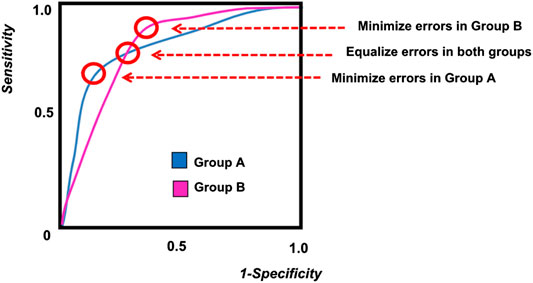
Figure 16.11: Receiver Operating Characteristic (ROC) Curves for Two Groups. (Figure reprinted from Fletcher et al. (2021), Figure 2, p. 3. Fletcher, R. R., Nakeshimana, A., & Olubeko, O. (2021). Addressing fairness, bias, and appropriate use of artificial intelligence and machine learning in global health. Frontiers in Artificial Intelligence, 3(116). https://doi.org/10.3389/frai.2020.561802)
It is not possible to meet all three types of fairness simultaneously (i.e., equal selection rates, sensitivity, and specificity across groups) unless the base rates are the same across groups or the selection is perfectly accurate (Fletcher et al., 2021). In the medical context, equal odds is the most common approach to fairness. However, using the cutoff associated with equal odds typically reduces overall classification accuracy. And, changing the cutoff for specific groups can lead to negative consequences. In the case that equal odds results in a classification accuracy that is too low, it may be worth considering using separate assessment procedures/tests for each group. In general, it is best to follow one of these approaches to fairness. It is difficult to get right, so try to minimize negative impact. Many fairness supporters argue for simpler rules. In the 1991 Civil Rights Act, score adjustments based on race, gender, and ethnicity (e.g., within-race norming or race-conscious score adjustments) were made illegal in personnel selection (L. S. Gottfredson, 1994).
Another perspective to fairness is that selection procedures should predict job performance and if they are correlated with any group membership (e.g., race, socioeconomic status, or gender), the test should not be used (Helms, 2006). That is, according to Helms, we should not use any test that assesses anything other than the construct of interest (job performance). Unfortunately, however, no measures like this exist. Every measure assesses multiple things, and factors such as poverty can have long-lasting impacts across many domains.
Another perspective to fairness is to make the selection procedures equal the number of successes within each group (Thorndike, 1971). According to this perspective, if you want to do selection, you should hire all people, then look at job performance. If among successful employees, 60% are White and 40% are Black, then set this selection rate for each group (i.e., hiring 80% White individuals and 20% Black individuals is not okay). According to this perspective, a selection system is only fair if the majority–minority differences on the selection device used are equal in magnitude to majority–minority differences in job performance. Selection criteria should be made based on prior distributions of success rates. However, you likely will not ever really know the true base rate in these situations. No one uses this approach because you would have a period where you have to accept everyone to find the percent that works. Also, this would only work in a narrow window of time because the selection pool changes over time.
There are lots of groups and subgroups. Ensuring fairness is very complex, and there is no way to accomplish the goal of being equally fair to all people. Therefore, do the best you can and try to minimize negative impact.
16.5 Correcting For Bias
16.5.1 What to Do When Detecting Bias
When examining item bias (using differential item functioning/DIF or measurement non-invariance) with many items (or measures) across many groups, there can be many tests, which will make it likely that DIF/non-invariance will be detected, especially with a large sample. Some detected DIF may be artificial or trivial, but other DIF may be real and important to address. It is important to consider how you will proceed when detecting DIF/non-invariance. Considerations of effect size and theory can be important for evaluating the DIF/non-invariance and whether it is negligible or important to address.
When detecting bias, there are several steps to take. First, consider what the bias indicates. Does the bias present adverse impact for a minority group? For what reasons might the bias exist? Second, examine the effect size of the bias. If the effects are small, if the bias does not present adverse impact for a minority group, and if there is no compelling theoretical reason for the bias, the bias might not be sufficient to scrap the instrument for the population. Some detected bias may be artificial, but other bias may be real. Gender and cultural differences have shown a number of statistically significant effects for a number of different assessment purposes, but many of the observed effects are quite small and likely trivial, and they do not present compelling reasons to change the assessment (Youngstrom & Van Meter, 2016).
However, if you find bias, correct for it! There are a number of score adjustment and non-score adjustment approaches to correct for bias, as described in Sections 16.5.2 and 16.5.3. If the bias occurs at the item level (e.g., test structure bias), it is generally recommended to remove or resolve items that show non-negligible bias. There are three primary options: (1) drop the item for both groups, (2) drop the item for one group but keep it for the other group, or (3) freely estimate the parameters for the item across groups. Addressing items that show larger bias can also reduce artificial bias in other items (Hagquist & Andrich, 2017). Thus, researchers are encouraged to handle item bias sequentially from high to low in magnitude. If the bias occurs at the test score level (e.g., predictive bias), score adjustments may be considered.
There are situations measurement invariance across time may not be expected (and may thus be problematic to require). For instance, if there is a treatment that occurs between two measurement occasions, the factor structure might change due to the treatment rather than due to the mere passage of time. Thus, it would be helpful to know whether the instrument shows measurement invariance across a similar timeframe when no treatment is occurring. Another situation where measurement invariance across time may not be expected is when the construct shows heterotypic continuity (Petersen et al., 2020). If the construct changes in its behavioral manifestation with development, then measurement invariance may not be expected across wide spans of time.
If you do not correct for bias, consider the impact of the test, procedure, and selection procedure when interpreting scores. Interpret scores with caution and provide necessary caveats in resulting papers or reports regarding the interpretations in question. In sum, it is important to examine the possibility of bias—it is important to consider how much “erroneous junk” you are introducing into your research.
16.5.2 Score Adjustment to Correct for Bias
Score adjustment involves adjusting scores for a particular group or groups.
16.5.2.1 Why Adjust Scores?
There may be several reasons to adjust scores for various groups in a given situation. First, there may be social goals to adjust scores. For example, we may want our selection device to yield personnel that better represent the nation or region, including diversity of genders, races, majors, social classes, etc. Score adjustments are typically discussed with respect to racial minority differences due to historical and systemic inequities. Our society aims to provide equal opportunity, including the opportunity to gain a fair share (i.e., proportional representation) of jobs. A diversity of perspectives in a job is a strength; a diversity of perspectives can lead to greater creativity and improved problem-solving. A second potential reason that we may want to apply score adjustment is to correct for bias. A third potential reason that we may want to apply score adjustment is to improve the fairness of a test.
16.5.2.2 Types of Score Adjustment
There are a number of potential techniques that have been used in attempts to correct for bias, i.e., to reduce negative impact of the test on an under-represented group. What is considered an under-represented group may depend on the context. For instance, men are under-represented compared to women as nurses, preschool teachers, and college students. However, men may not face the same systemic challenges compared to women, so even though men may show under-representation in some domains, it is arguable whether scores should be adjusted to increase their representation. Techniques for score adjustment include:
- Bonus points
- Within-group norming
- Separate cutoffs
- Top-down selection from different lists
- Banding
- Banding with bonus points
- Sliding band
- Separate tests
- Item elimination based on group differences
16.5.2.2.1 Bonus Points
Providing bonus points involves adding a constant number of points to the scores of all individuals who are members of a particular group with the goal of eliminating or reducing group differences. Bonus points is used to correct for predictive bias differences in intercepts between groups. An example of bonus points is military veterans in placement for civil service jobs—points are added to the initial score for all veterans (e.g., add 5 points to test scores of all veterans). An example of using bonus points as a score adjustment is depicted in Figure 16.12.
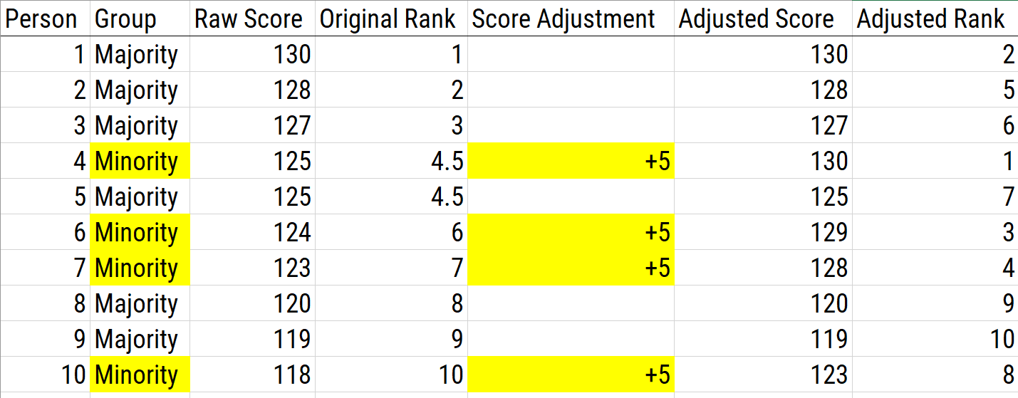
Figure 16.12: Using Bonus Points as a Scoring Adjustment.
There are several pros of bonus points. If the distribution of each group is the same, this will effectively reduce group differences. Moreover, it is a simple way of impacting test selection and procedure without changing the test, which is therefore a great advantage. There are several cons of bonus points. If there are differences in group standard deviations, adding bonus points may not actually correct for bias. The use of bonus points also obscures what is actually being done to scores, so other methods like using separate cutoffs may be more explicit. In addition, the simplicity of bonus points is also a great disadvantage because it is easily understood and often not viewed as “fair” because some people are getting extra points that others do not.
16.5.2.2.2 Within-Group Norming
A norm is the standard of performance that a person’s performance can be compared to. Within-group norming treats the person’s group in the sample as the norm. Within-group norming converts an individual’s score to standardized scores (e.g., T scores) or percentiles within one’s own group. Then, the people are selected based on the highest standard scores across groups. Withing-group norming is used to correct for predictive bias differences in slopes between groups. An example of using within-group norming as a score adjustment is depicted in Figure 16.13.
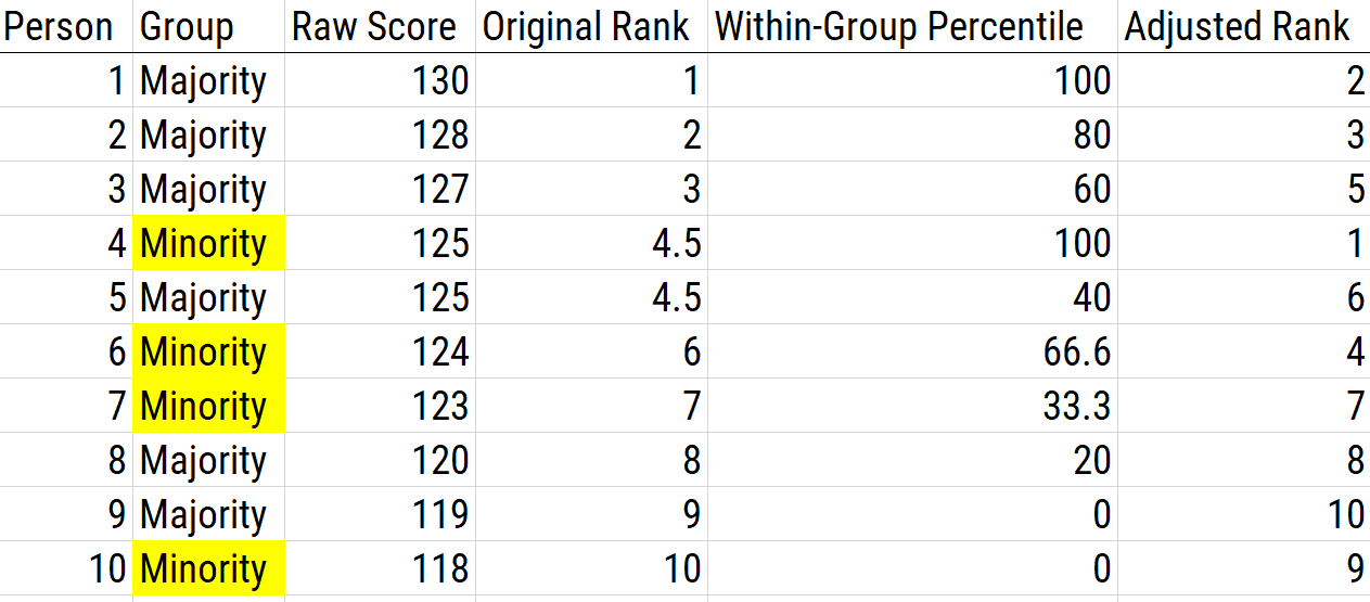
Figure 16.13: Using Within-Group Norming as a Scoring Adjustment.
There are several pros of within-group norming. First, it accounts for differences in group standard deviations and means, so it does not have the same problem as bonus points and is generally more effective at eliminating adverse impact compared to bonus points. Second, some general (non-group-specific) norms are clearly irrelevant for characterizing a person’s functioning. Group-specific norms aim to describe a person’s performance relative to people with a similar background, thus potentially reducing cultural bias. Third, group-specific norms may better reflect cultural, educational, socioeconomic, and other factors that may influence a person’s score (Burlew et al., 2019). Fourth, group-specific norms may increase specificity, and reduce over-pathologizing by preventing giving a diagnosis to people who might not show a condition (Manly & Echemendia, 2007).
There are several cons of within-group norming. First, group differences could be maintained if one decides to norm based on a reference sample or, when scores are skewed, a local sample, especially when using standardized scores. However, percentile scores will consistently eliminate adverse impact. Second, using group-specific norms may obscure background variables that explain underlying reasons for group-related differences in test performance (Manly, 2005; Manly & Echemendia, 2007). Third, group-specific norms do not address the problem if the measure shows test bias (Burlew et al., 2019). Fourth, group-specific norms may reduce sensitivity to detect conditions (Manly & Echemendia, 2007). For instance, they may prevent people from getting treatment who would benefit. It is worth noting that within-group norming on the basis of sex, gender, and ethnicity is illegal for the basis of personnel selection according to the 1991 Civil Rights Act.
As an example of within-group norming, the National Football League used to use race-norming for identification of concussions. The effect of race-norming, however, was that it lowered Black players’ concussion risk scores, which prevented many Black players from being identified as having sustained a concussion and from receiving needed treatment. Race-norming compared the Black football players cognitive test scores to group-specific norms: the cognitive test scores of Black people in the general population (not to common norms). Using Black-specific norms assumed that Black football players showed lower cognitive ability than other groups, so a low cognitive ability score for a Black player was less likely to be flagged as concerning. Thus, the race-specific norms led to lower identified rates of concussions among Black football players compared to White football players. Due to the adverse impact, Black players sued the National Football League, and the league stopped the controversial practice of race-norming for identification of concussion (https://www.washingtonpost.com/sports/2021/06/03/nfl-concussion-settlement-race-norming/; archived at https://perma.cc/KN3L-5Z7R).
A common question is whether to use group-specific norms or common norms. Group-specific norms are a controversial practice, and the answer depends. If you are interested in a person’s absolute functioning (e.g., for determining whether someone is concussed or whether they are suitable to drive), recommendations are to use common norms, not group-specific norms (Barrash et al., 2010; Silverberg & Millis, 2009). If, by contrast, you are interested in a person’s relative functioning compared to a specific group, within-group norming could make sense if there is an appropriate reference group. The question about which norms to use are complex, and psychologists should evaluate the cost and benefit of each norm, and use the norm with the greatest benefit and the least cost for the client (Manly & Echemendia, 2007).
16.5.2.2.3 Separate Cutoffs
Using separate cutoffs involves using a separate cutoff score per group and selecting the top number from each group. That is, using separate cutoffs involves using different criteria for each group. Using separate cutoffs functions the same as adding bonus points, but it has greater transparency—i.e., you are lowering the standard for one group compared to another group. An example of using separate cutoffs as a score adjustment is depicted in Figure 16.14.
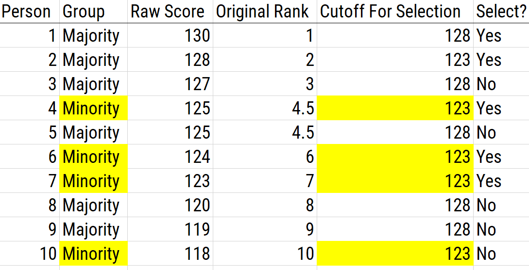
Figure 16.14: Using Separate Cutoffs as a Scoring Adjustment. In this example, the cutoff for the majority group is 128; the cutoff for the minority group is 123.
16.5.2.2.4 Top-Down Selection from Different Lists
Top-down selection from different lists involves taking the best from two different lists according to a preset rule as to how many to select from each group. Top-down selection from different lists functions the same as within-group norming. An example of using top-down selection from different lists as a score adjustment is depicted in Figure 16.15.
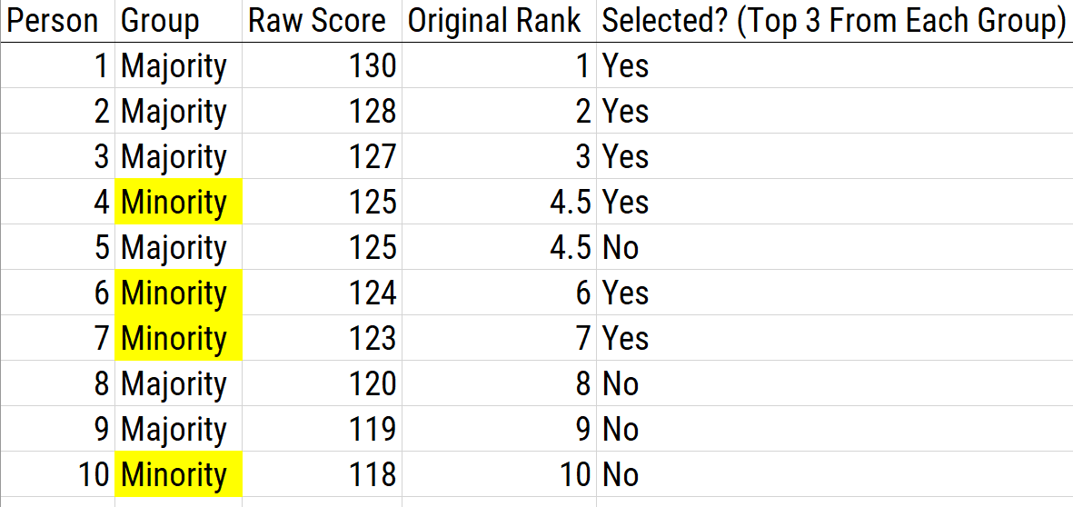
Figure 16.15: Using Top-Down Selection From Different Lists as a Scoring Adjustment. In this example, the top three candidates are selected from each group.
16.5.2.2.5 Banding
Banding uses a tier system that is based on the assumption that individuals within a specific score range are regarded as having equivalent scores. So that we do not over-estimate small score differences, scores within the same band are seen as equivalent—and the order of selection within the band can be modified depending on selection goals. The standard error of measurement (SEM) is used to estimate the precision (reliability) of the test scores, and it is used as the width of the band.
Consider an example: if a person received a score with confidence interval of 18–22, then scores between 18 to 22 are not necessarily different due to random fluctuation (measurement error). Therefore, scores in that range are considered the same, and we take a band of scores. However, banding by itself may not result in increased selection of lower scoring groups. The band provides a subsample of applicants so that we can use other criteria (other than the test) to select a candidate. Giving “minority preference” involves selecting members of minority group in a given band before selecting members of the majority group. An example of using banding as a score adjustment is depicted in Figure 16.16.
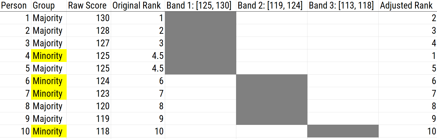
Figure 16.16: Using Banding as a Scoring Adjustment.
The problem with banding is that bands are set by the standard error of measurement: you can select the first group from the first band, but then whom do you select after the first band? There is no rationale where to “stop” the band because there are indistinguishable scores on the edges of each band to the next band. That is, 17 is indistinguishable from 18 (in terms of its confidence interval), 16 is indistinguishable from 17, and so on. Therefore, banding works okay for the top scores, but if you are going to hire a lot of candidates, it is a problem. A solution to this problem with banding is to use a sliding band, as described later.
16.5.2.2.6 Banding with Bonus Points
Banding is often used with bonus points to reduce the negative impact for minority groups. An example of using banding with bonus points as a score adjustment is depicted in Figure 16.17.
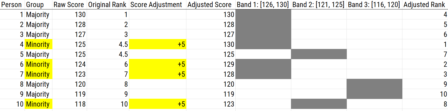
Figure 16.17: Using Banding With Bonus Points as a Scoring Adjustment.
16.5.2.2.7 Sliding Band
Using a sliding band is a solution to the problem of which bands to use when using banding. Using a sliding band can help increase the number of minorities selected. Using the top band, you select all members of a minority group in the top band, then select members of the majority group with the top score of the band, then slide the band down (based on SEM), and repeat. You work your way down with bands though groups that are indistinguishable based on SEM, until getting a cell needed to select a relevant candidate.
For instance, if the top score is 22 and the SEM is 4 points, the first band would be: [18, 22]. Here is how you would proceed:
- Select the minority group members who have a score between 18 to 22.
- Select the majority group members who have a score of 22.
- Slide the band down based on the SEM to the next highest score: [17, 21].
- Select the minority group members who have a score between 17 to 21.
- Select the majority group members who have a score of 21.
- Slide the band down based on the SEM to the next highest score: [16, 20].
- …
- And so on
An example of using a sliding band as a score adjustment is depicted in Figure 16.18.
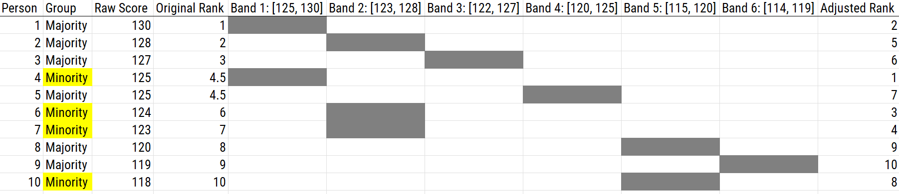
Figure 16.18: Using a Sliding Band as a Scoring Adjustment.
In sum, using a sliding band, scores that are not significantly lower than the highest remaining score should not be treated as different. Using a sliding band has the same effects on decisions as bonus points that are the width of the band. For example, if the SEM is 3, it has the same decisions as bonus points of 3; therefore, any scores within 3 of the highest score are now considered equal.
A sliding band is popular because of its scientific and statistical rationale. Also, it is more confusing and, therefore, preferred by some because it may be less likely to be sued. However, a sliding band may not always eliminate adverse impact. A sliding band has never been overturned in court (or at least, not yet).
16.5.2.2.8 Separate Tests
Using separate tests for each group is another option to reduce bias. For instance, you might use one test for the majority group and a different test for the minority group, making sure that each test is valid for the relevant group. Using separate tests is an extreme version of top-down selection and within-group norming. Using separate tests would be an option if a measure shows different slopes predictive bias.
One way of developing separate tests is to use empirical keying by group: different items for each group are selected based on each item’s association with the criterion in each group. Empirical keying is an example of dustbowl empiricism (i.e., relying on empiricism rather than theory). However, theory can also inform the item selection.
16.5.2.2.9 Item Elimination based on Group Differences
Items that show large group differences in scores can be eliminated from the test. If you remove enough items showing differences between groups, you can get similar scores between groups and can get equal group selection. A problem of item elimination based on group differences is that if you get rid of predictive items, then two goals, equal selection and predictive power, are not met. If you use this method, you often have to be willing for the measure to show decreases in predictive power.
16.5.2.3 Use of Score Adjustment
Score adjustment can be used in a number of different domains, including tests of aptitude and intelligence. Score adjustment also comes up in other areas. For example, the number of drinks it takes to be considered binge drinking differs between men (five) and women (four). Although the list of score adjustment options is long, they all really reduce to two ways:
Bonus points and within-group norming are the techniques that are most often used in the real world. These techniques differ in their degree of obscurity—i.e., confusion that is caused not for scientific reasons, but for social, political, and dissemination and implementation reasons. Often procedures that are hard to understand are preferred because it is hard to argue against, critique, or game the system. Basically, you have two options for score adjustment. One option is to adjust scores by raising scores in one group or lowering the criterion in one group. The second primary option is to renorm or change the scores. In sum, you can change the scores, or you can change the decisions you make based on the scores.
16.5.3 Other Ways to Correct for Bias
Because score adjustment is controversial, it is also important to consider other potential ways to correct for bias that do not involve score adjustment. Strategies other than score adjustment to correct for bias are described by Sackett et al. (2001).
16.5.3.1 Use Multiple Predictors
In general, high-stakes decisions should not be made based on the results from one test. So, for instance, do not make hiring decisions based just on aptitude assessments. For example, college admissions decisions are not made just based on SAT scores, but also one’s grades, personal statement, extracurricular activities, letters of recommendation, etc. Using multiple predictors works best when the predictors are not correlated with the assessment that has adverse impact, which is difficult to achieve.
There are larger majority–minority subgroup differences in verbal and cognitive ability tests than in noncognitive skills (e.g., motivation, personality, and interpersonal skills). So, it is important to include assessment of relevant noncognitive skills. Include as many relevant aspects of the construct as possible for content validity. For a job, consider as many factors as possible that are relevant for success, e.g., cognitive and noncognitive abilities.
16.5.3.2 Change the Criterion
Another option is to change the criterion so that the predictive validity of tests is less skewed. It may be that the selection instrument is not biased but the way in which we are thinking about selection procedures is biased. For example, for judging the quality of universities, there are many different criteria we could use. It could be valuable to examine the various criteria, and you might find what is driving adverse effects.
16.5.3.3 Remove Biased Items
Using item response theory or confirmatory factor analysis, you can identify items that function differently across groups (i.e., differential item functioning/DIF or measurement non-invariance). For instance, you can identify items that show different discrimination/factor loadings or difficulty/intercepts by group. You do not just want to remove items that show mean-level differences in scores (or different rates of endorsement) for one group than another, because there may be true group differences in their level on particular items. If an item is clearly invalid in one group but valid in another group, another option is to keep the item in one group, and to remove it in another group.
Be careful when removing items because removing items can lead to poorer content validity—i.e., items may no longer be a representative set of the content of the construct. Removing items also reduces a measure’s reliability and ability to detect individual differences (Hagquist, 2019; Hagquist & Andrich, 2017). DIF effects tend to be small and inconsistent; removing items showing DIF may not have a big impact.
16.5.3.4 Resolve Biased Items
Another option, for items identified that show differential item functioning using IRT or measurement non-invariance using CFA, is to resolve instead of remove items. Resolving items involves allowing an item to have a different discrimination/factor loading and/or difficulty/intercept parameter for each group. Allowing item parameters to differ across groups has a very small effect on reliability and person separation, so it can be preferable to removing items (Hagquist, 2019; Hagquist & Andrich, 2017).
16.5.3.5 Use Alternative Modes of Testing
Another option is to use alternative modes of testing. For example, you could use audio or video to present test items, rather than requiring a person to read the items, or write answers. Typical testing and computerized exams are oriented toward the upper-middle class, which is therefore a procedure problem! McClelland’s (1973) argument is that we need more real-life testing. Real-life testing could help address stereotype threats and the effects of learning disabilities. However, testing in different modalities could change the construct(s) being assessed.
16.5.3.6 Use Work Records
Using work records is based on McClelland’s (1973) argument to use more realistic and authentic assessments of job-relevant abilities. Evidence on the value of work records for personnel selection is mixed. In some cases, use of work records can actually increase adverse impact on under-represented groups because the primary group typically already has an idea of how to get into the relevant job or is already in the relevant job; therefore, they have a leg up. It would be acceptable to use work records if you trained people first and then tested, but no one spends the time to do this.
16.5.3.7 Increase Time Limit
Another option is to allot people more testing time, as long as doing so does not change the construct. Time limits often lead to greater measurement error because scores conflate pace and quality of work. Increasing time limits requires convincing stakeholders that job performance is typically not “how fast you do things” but “how well you do them”—i.e., that time does not correlate with outcome of interest. The utility of increasing time limits depends on the domain. In some domains, efficiency is crucial (e.g., medicine, pilot). Increasing time limits is not that effective in reducing group differences, and it may actually increase group differences.
16.5.3.8 Use Motivation Sets
Using motivation sets involves finding ways to increase testing motivation for minority groups. It is probably an error to think that a test assesses just aptitude; therefore, we should also consider an individual’s motivation to test. Thus, part of the score has to do with ability and some of the score has to do with motivation. You should try to maximize each examinee’s motivation, so that the person’s score on the measure better captures their true ability score. Motivation sets could include, for example, using more realistic test stimuli that are clearly applicable to the school or job requirements (i.e., that have face validity) to motivate all test takers.
16.5.3.9 Use Instructional Sets
Using instructional sets involves coaching and training. For instance, you could inform examinees about the test content, provide study materials, and recommend test-taking strategies. This could narrow the gap between groups because there is an implicit assumption that the primary group already has “light” training. Using instructional sets aims to reduce error variance due to test anxiety, unfamiliar test format, and poor test-taking skills.
Giving minority groups better access to test preparation is based on the assumption that group differences emerge because of different access to test preparation materials. This could theoretically help to systematically reduce test score differences across groups. Standardized tests like the SAT/GRE/LSAT/GMAT/MCAT, etc. embrace coaching/training. For instance, the organization ETS gives training materials for free. After training, scores on standardized tests show some but minimal improvement. In general, training yields some improvement on quantitative subscales but minimal change on verbal subscales. However, the improvements tend to apply across groups, and they do not seem to lessen group differences in scores.
16.6 Getting Started
16.6.1 Load Libraries
Code
library("petersenlab") #to install: install.packages("remotes"); remotes::install_github("DevPsyLab/petersenlab")
library("lavaan")
library("semTools")
library("semPlot")
library("mirt")
library("dmacs") #to install: install.packages("remotes"); remotes::install_github("ddueber/dmacs")
library("strucchange")
library("MOTE")
library("tidyverse")
library("here")
library("tinytex")
16.6.2 Prepare Data
16.6.2.1 Load Data
cnlsy is a subset of a data set from the Children of the National Longitudinal Survey of Youth Survey (CNLSY).
The CNLSY is a publicly available longitudinal data set provided by the Bureau of Labor Statistics (https://perma.cc/EH38-HDRN).
The CNLSY data file for these examples is located on the book’s page of the Open Science Framework (https://osf.io/3pwza).
16.6.2.2 Simulate Data
For reproducibility, I set the seed below. Using the same seed will yield the same answer every time. There is nothing special about this particular seed.
Code
sampleSize <- 4000

set.seed(52242)

mydataBias <- data.frame(
  ID = 1:sampleSize,
  group = factor(c("male","female"),
                 levels = c("male","female")),
  unbiasedPredictor1 = NA,
  unbiasedPredictor2 = NA,
  unbiasedPredictor3 = NA,
  unbiasedCriterion1 = NA,
  unbiasedCriterion2 = NA,
  unbiasedCriterion3 = NA,
  predictor = rnorm(sampleSize, mean = 100, sd = 15),
  criterion1 = NA,
  criterion2 = NA,
  criterion3 = NA,
  criterion4 = NA,
  criterion5 = NA)

mydataBias$unbiasedPredictor1 <- rnorm(sampleSize, mean = 100, sd = 15)
mydataBias$unbiasedPredictor2[which(mydataBias$group == "male")] <-
  rnorm(length(which(mydataBias$group == "male")), mean = 70, sd = 15)
mydataBias$unbiasedPredictor2[which(mydataBias$group == "female")] <-
  rnorm(length(which(mydataBias$group == "female")), mean = 130, sd = 15)
mydataBias$unbiasedPredictor3[which(mydataBias$group == "male")] <-
  rnorm(length(which(mydataBias$group == "male")), mean = 130, sd = 15)
mydataBias$unbiasedPredictor3[which(mydataBias$group == "female")] <-
  rnorm(length(which(mydataBias$group == "female")), mean = 70, sd = 15)

mydataBias$unbiasedCriterion1 <- 1 * mydataBias$unbiasedPredictor1 +
  rnorm(sampleSize, mean = 0, sd = 15)
mydataBias$unbiasedCriterion2 <- 1 * mydataBias$unbiasedPredictor2 +
  rnorm(sampleSize, mean = 0, sd = 15)
mydataBias$unbiasedCriterion3 <- 1 * mydataBias$unbiasedPredictor3 +
  rnorm(sampleSize, mean = 0, sd = 15)

mydataBias$criterion1[which(mydataBias$group == "male")] <-
  .7 * mydataBias$predictor[which(mydataBias$group == "male")] +
  rnorm(length(which(mydataBias$group == "male")), mean = 0, sd = 5)
mydataBias$criterion1[which(mydataBias$group == "female")] <-
  .7 * mydataBias$predictor[which(mydataBias$group == "female")] +
  rnorm(length(which(mydataBias$group == "female")), mean = 0, sd = 5)
mydataBias$criterion2[which(mydataBias$group == "male")] <-
  .7 * mydataBias$predictor[which(mydataBias$group == "male")] +
  rnorm(length(which(mydataBias$group == "male")), mean = 10, sd = 5)
mydataBias$criterion2[which(mydataBias$group == "female")] <-
  .7 * mydataBias$predictor[which(mydataBias$group == "female")] +
  rnorm(length(which(mydataBias$group == "female")), mean = 0, sd = 5)
mydataBias$criterion3[which(mydataBias$group == "male")] <-
  .7 * mydataBias$predictor[which(mydataBias$group == "male")] +
  rnorm(length(which(mydataBias$group == "male")), mean = 0, sd = 5)
mydataBias$criterion3[which(mydataBias$group == "female")] <-
  .3 * mydataBias$predictor[which(mydataBias$group == "female")] +
  rnorm(length(which(mydataBias$group == "female")), mean = 0, sd = 5)
mydataBias$criterion4[which(mydataBias$group == "male")] <-
  .7 * mydataBias$predictor[which(mydataBias$group == "male")] +
  rnorm(length(which(mydataBias$group == "male")), mean = 0, sd = 5)
mydataBias$criterion4[which(mydataBias$group == "female")] <-
  .3 * mydataBias$predictor[which(mydataBias$group == "female")] +
  rnorm(length(which(mydataBias$group == "female")), mean = 30, sd = 5)
mydataBias$criterion5[which(mydataBias$group == "male")] <-
  .7 * mydataBias$predictor[which(mydataBias$group == "male")] +
  rnorm(length(which(mydataBias$group == "male")), mean = 0, sd = 30)
mydataBias$criterion5[which(mydataBias$group == "female")] <-
  .7 * mydataBias$predictor[which(mydataBias$group == "female")] +
  rnorm(length(which(mydataBias$group == "female")), mean = 0, sd = 5)
16.6.2.3 Add Missing Data
Adding missing data to dataframes helps make examples more realistic to real-life data and helps you get in the habit of programming to account for missing data.
HolzingerSwineford1939 is a data set from the lavaan package (Rosseel et al., 2022) that contains mental ability test scores (x1–x9) for seventh- and eighth-grade children.
Code
varNames <- names(mydataBias)
dimensionsDf <- dim(mydataBias[,-c(1,2)])
unlistedDf <- unlist(mydataBias[,-c(1,2)])
unlistedDf[sample(
  1:length(unlistedDf),
  size = .01 * length(unlistedDf))] <- NA
mydataBias <- cbind(
  mydataBias[,c("ID","group")],
  as.data.frame(
    matrix(
      unlistedDf,
      ncol = dimensionsDf[2])))
names(mydataBias) <- varNames

data("HolzingerSwineford1939")
varNames <- names(HolzingerSwineford1939)
dimensionsDf <- dim(HolzingerSwineford1939[,paste("x", 1:9, sep = "")])
unlistedDf <- unlist(HolzingerSwineford1939[,paste("x", 1:9, sep = "")])
unlistedDf[sample(
  1:length(unlistedDf),
  size = .01 * length(unlistedDf))] <- NA
HolzingerSwineford1939 <- cbind(
  HolzingerSwineford1939[,1:6],
  as.data.frame(matrix(
    unlistedDf,
    ncol = dimensionsDf[2])))
names(HolzingerSwineford1939) <- varNames
16.7 Examples of Unbiased Tests (in Terms of Predictive Bias)
16.7.1 Unbiased test where males and females have equal means on predictor and criterion
Figure 16.19 depicts an example of an unbiased test where males and females have equal means on the predictor and criterion.
The test is unbiased because there are no significant differences in the regression lines (of predictor predicting criterion) between males and females.
Code
Call:
lm(formula = unbiasedCriterion1 ~ unbiasedPredictor1 + group +
    unbiasedPredictor1:group, data = mydataBias)

Residuals:
    Min      1Q  Median      3Q     Max
-54.623 -10.050  -0.025  10.373  66.811

Coefficients:
                                Estimate Std. Error t value Pr(>|t|)
(Intercept)                     0.930697   2.295058   0.406    0.685
unbiasedPredictor1              0.996976   0.022624  44.066   <2e-16 ***
groupfemale                    -1.165200   3.250481  -0.358    0.720
unbiasedPredictor1:groupfemale -0.004397   0.032115  -0.137    0.891
---
Signif. codes:  0 '***' 0.001 '**' 0.01 '*' 0.05 '.' 0.1 ' ' 1

Residual standard error: 15.13 on 3913 degrees of freedom
  (83 observations deleted due to missingness)
Multiple R-squared:  0.4963,    Adjusted R-squared:  0.496
F-statistic:  1285 on 3 and 3913 DF,  p-value: < 2.2e-16
Code
plot(
  unbiasedCriterion1 ~ unbiasedPredictor1,
  data = mydataBias,
  xlim = c(
    0,
    max(c(
      mydataBias$unbiasedCriterion1,
      mydataBias$unbiasedPredictor1),
      na.rm = TRUE)),
  ylim = c(
    0,
    max(c(
      mydataBias$criterion1,
      mydataBias$predictor),
      na.rm = TRUE)),
  type = "n",
  xlab = "predictor",
  ylab = "criterion")
points(
  mydataBias$unbiasedPredictor1[which(mydataBias$group == "male")],
  mydataBias$unbiasedCriterion1[which(mydataBias$group == "male")],
  pch = 20,
  col = "blue")
points(mydataBias$unbiasedPredictor1[which(mydataBias$group == "female")],
       mydataBias$unbiasedCriterion1[which(mydataBias$group == "female")],
       pch = 1,
       col = "red")
abline(lm(
  unbiasedCriterion1 ~ unbiasedPredictor1,
  data = mydataBias[which(mydataBias$group == "male"),]),
  lty = 1,
  col = "blue")
abline(lm(
  unbiasedCriterion1 ~ unbiasedPredictor1,
  data = mydataBias[which(mydataBias$group == "female"),]),
  lty = 2,
  col = "red")
legend(
  "bottomright",
  c("Male","Female"),
  lty = c(1,2),
  pch = c(20,1),
  col = c("blue","red"))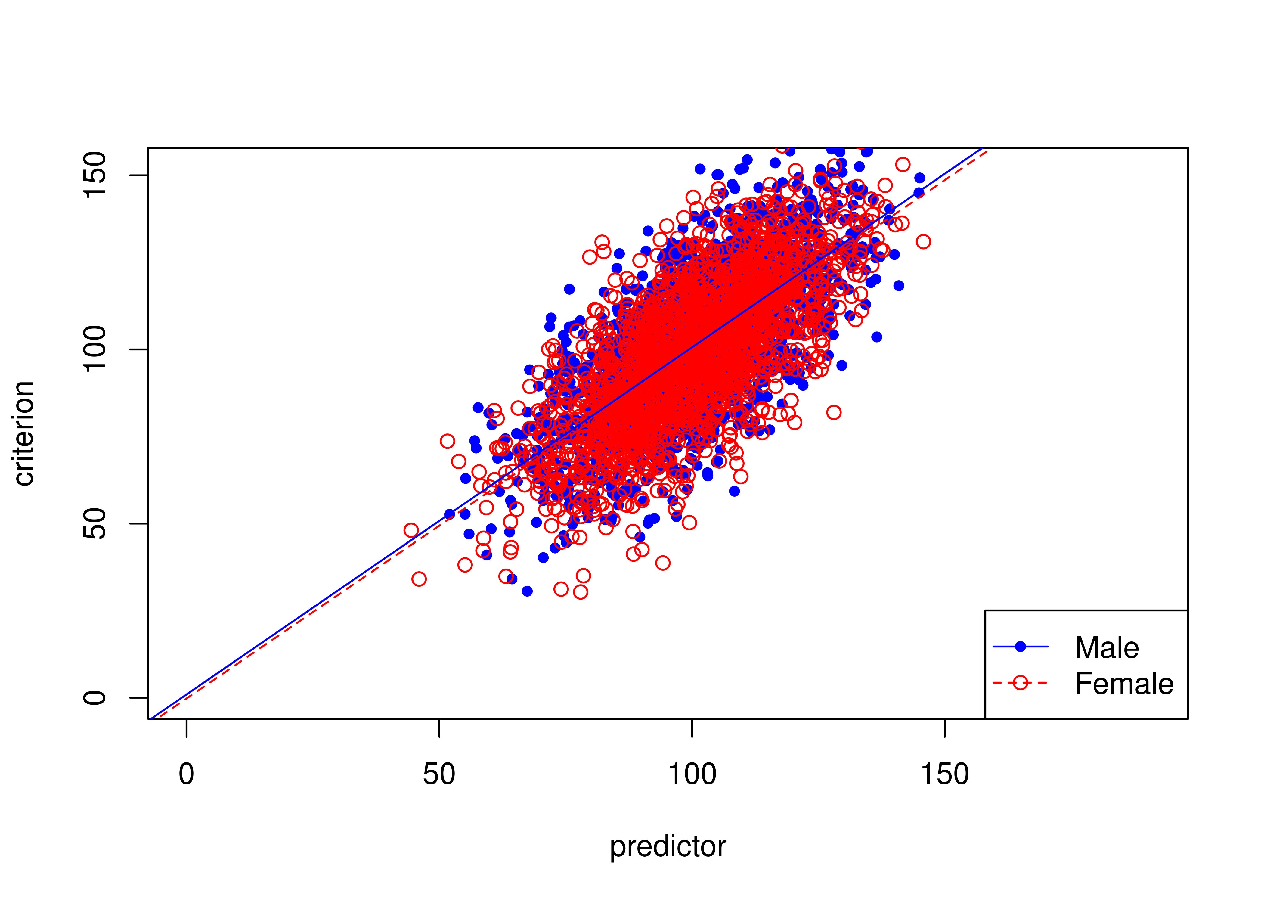
Figure 16.19: Unbiased Test Where Males and Females Have Equal Means on Predictor and Criterion.
16.7.2 Unbiased test where females have higher means than males on predictor and criterion
Figure 16.20 depicts an example of an unbiased test where females have higher means than males on the predictor and criterion.
The test is unbiased because there are no differences in the regression lines (of predictor predicting criterion) between males and females.
Code
Call:
lm(formula = unbiasedCriterion2 ~ unbiasedPredictor2 + group +
    unbiasedPredictor2:group, data = mydataBias)

Residuals:
    Min      1Q  Median      3Q     Max
-47.302  -9.989   0.010   9.860  53.791

Coefficients:
                               Estimate Std. Error t value Pr(>|t|)
(Intercept)                    -1.29332    1.57773  -0.820    0.412
unbiasedPredictor2              1.02006    0.02218  46.000   <2e-16 ***
groupfemale                     1.21294    3.28319   0.369    0.712
unbiasedPredictor2:groupfemale -0.01501    0.03125  -0.480    0.631
---
Signif. codes:  0 '***' 0.001 '**' 0.01 '*' 0.05 '.' 0.1 ' ' 1

Residual standard error: 14.81 on 3919 degrees of freedom
  (77 observations deleted due to missingness)
Multiple R-squared:  0.8412,    Adjusted R-squared:  0.8411
F-statistic:  6921 on 3 and 3919 DF,  p-value: < 2.2e-16
Code
plot(
  unbiasedCriterion2 ~ unbiasedPredictor2,
  data = mydataBias,
  xlim = c(
    0,
    max(c(
      mydataBias$unbiasedCriterion2,
      mydataBias$unbiasedPredictor2),
      na.rm = TRUE)),
  ylim = c(
    0,
    max(c(
      mydataBias$criterion1,
      mydataBias$predictor),
      na.rm = TRUE)),
  type = "n",
  xlab = "predictor",
  ylab = "criterion")
points(
  mydataBias$unbiasedPredictor2[which(mydataBias$group == "male")],
  mydataBias$unbiasedCriterion2[which(mydataBias$group == "male")],
  pch = 20,
  col = "blue")
points(
  mydataBias$unbiasedPredictor2[which(mydataBias$group == "female")],
  mydataBias$unbiasedCriterion2[which(mydataBias$group == "female")],
  pch = 1,
  col = "red")
abline(lm(
  unbiasedCriterion2 ~ unbiasedPredictor2,
  data = mydataBias[which(mydataBias$group == "male"),]),
  lty = 1,
  col = "blue")
abline(lm(
  unbiasedCriterion2 ~ unbiasedPredictor2,
  data = mydataBias[which(mydataBias$group == "female"),]),
  lty = 2,
  col = "red")
legend(
  "bottomright",
  c("Male","Female"),
  lty = c(1,2),
  pch = c(20,1),
  col = c("blue","red"))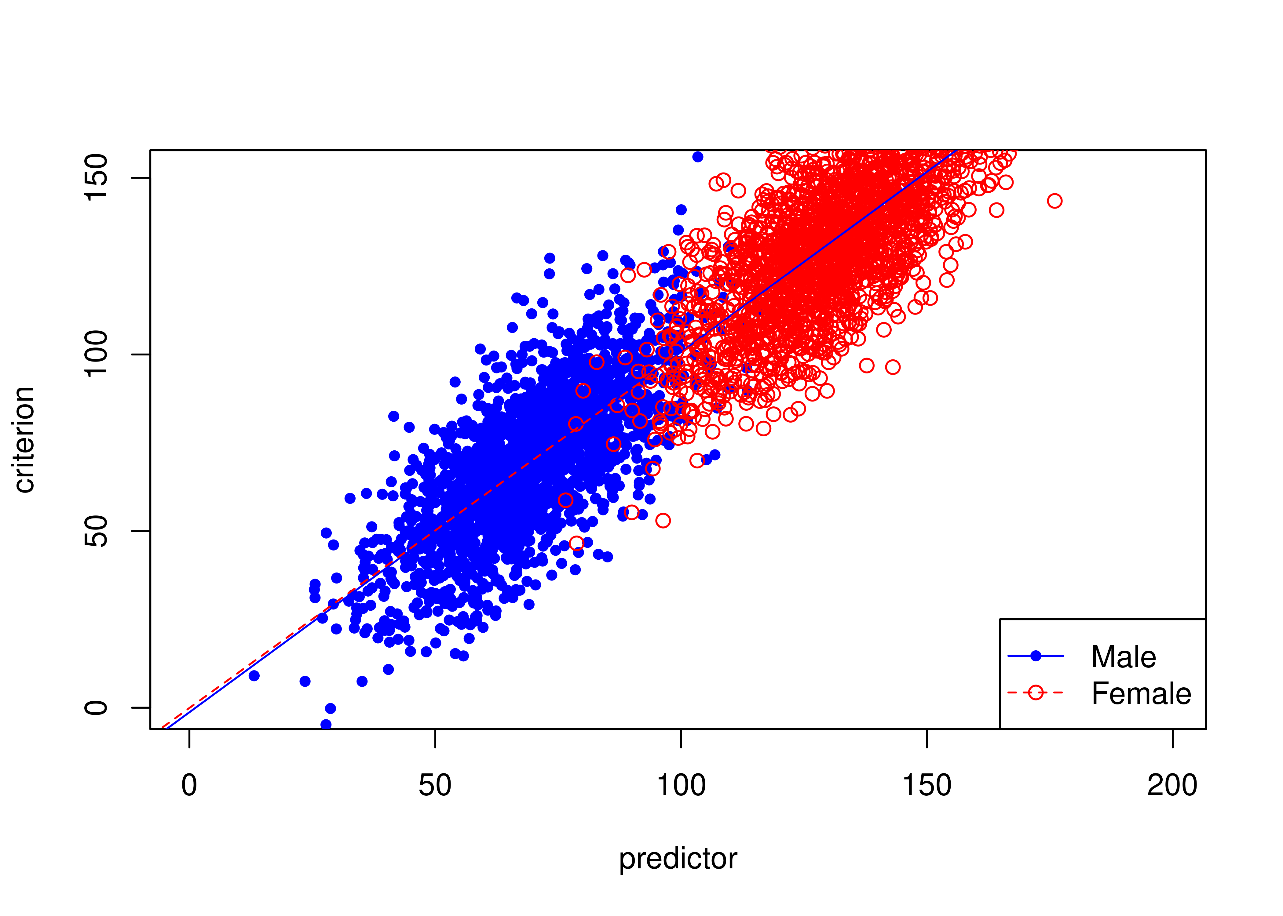
Figure 16.20: Unbiased Test Where Females Have Higher Means Than Males on Predictor and Criterion.
16.7.3 Unbiased test where males have higher means than females on predictor and criterion
Figure 16.21 depicts an example of an unbiased test where males have higher means than females on the predictor and criterion.
The test is unbiased because there are no differences in the regression lines (of predictor predicting criterion) between males and females.
Code
Call:
lm(formula = unbiasedCriterion3 ~ unbiasedPredictor3 + group +
    unbiasedPredictor3:group, data = mydataBias)

Residuals:
    Min      1Q  Median      3Q     Max
-48.613 -10.115  -0.068   9.598  57.126

Coefficients:
                               Estimate Std. Error t value Pr(>|t|)
(Intercept)                    -1.68352    2.84985  -0.591    0.555
unbiasedPredictor3              1.01072    0.02179  46.375   <2e-16 ***
groupfemale                     1.42842    3.26227   0.438    0.662
unbiasedPredictor3:groupfemale -0.01187    0.03109  -0.382    0.703
---
Signif. codes:  0 '***' 0.001 '**' 0.01 '*' 0.05 '.' 0.1 ' ' 1

Residual standard error: 14.82 on 3916 degrees of freedom
  (80 observations deleted due to missingness)
Multiple R-squared:  0.8376,    Adjusted R-squared:  0.8375
F-statistic:  6732 on 3 and 3916 DF,  p-value: < 2.2e-16
Code
plot(
  unbiasedCriterion3 ~ unbiasedPredictor3,
  data = mydataBias,
  xlim = c(
    0,
    max(c(
      mydataBias$unbiasedCriterion3,
      mydataBias$unbiasedPredictor3),
      na.rm = TRUE)),
  ylim = c(0, max(c(
    mydataBias$criterion1,
    mydataBias$predictor),
    na.rm = TRUE)),
  type = "n",
  xlab = "predictor",
  ylab = "criterion")
points(
  mydataBias$unbiasedPredictor3[which(mydataBias$group == "male")],
  mydataBias$unbiasedCriterion3[which(mydataBias$group == "male")],
  pch = 20,
  col = "blue")
points(
  mydataBias$unbiasedPredictor3[which(mydataBias$group == "female")],
  mydataBias$unbiasedCriterion3[which(mydataBias$group == "female")],
  pch = 1,
  col = "red")
abline(lm(
  unbiasedCriterion3 ~ unbiasedPredictor3,
  data = mydataBias[which(mydataBias$group == "male"),]),
  lty = 1,
  col = "blue")
abline(lm(
  unbiasedCriterion3 ~ unbiasedPredictor3,
  data = mydataBias[which(mydataBias$group == "female"),]),
  lty = 2,
  col = "red")
legend(
  "bottomright",
  c("Male","Female"),
  lty = c(1,2),
  pch = c(20,1),
  col = c("blue","red"))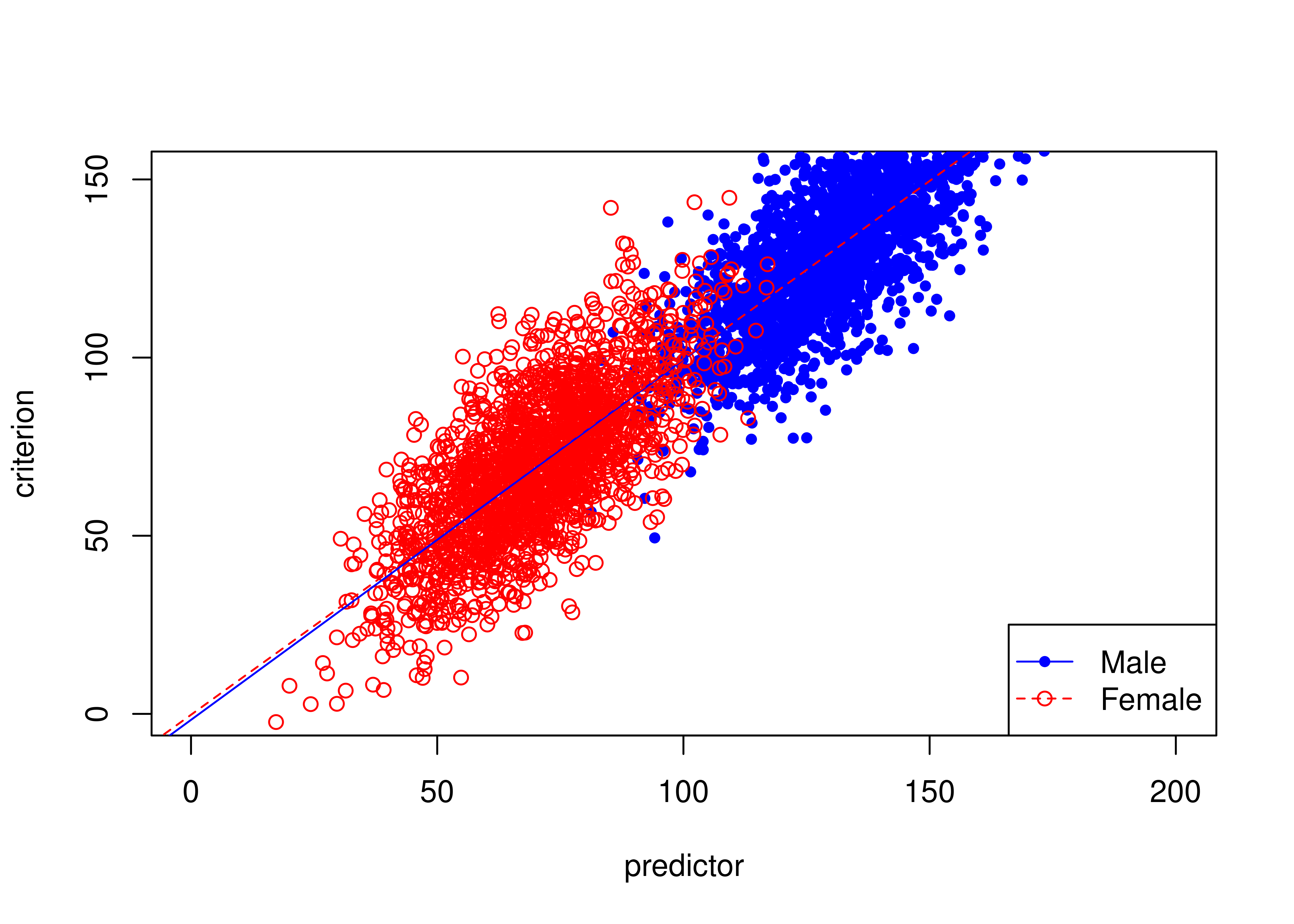
Figure 16.21: Unbiased Test Where Males Have Higher Means Than Females on Predictor and Criterion.
16.8 Predictive Bias: Different Regression Lines
16.8.1 Example of unbiased prediction (no differences in intercepts or slopes)
Figure 16.22 depicts an example of an unbiased test where males and females have equal means on the predictor and criterion.
The test is unbiased because there are no differences in the regression lines (of predictor predicting criterion1) between males and females.
Call:
lm(formula = criterion1 ~ predictor + group + predictor:group,
    data = mydataBias)

Residuals:
    Min      1Q  Median      3Q     Max
-18.831  -3.338   0.004   3.330  19.335

Coefficients:
                       Estimate Std. Error t value Pr(>|t|)
(Intercept)           -0.264357   0.747269  -0.354    0.724
predictor              0.701726   0.007370  95.207   <2e-16 ***
groupfemale           -0.515860   1.059267  -0.487    0.626
predictor:groupfemale  0.006002   0.010476   0.573    0.567
---
Signif. codes:  0 '***' 0.001 '**' 0.01 '*' 0.05 '.' 0.1 ' ' 1

Residual standard error: 4.952 on 3908 degrees of freedom
  (88 observations deleted due to missingness)
Multiple R-squared:  0.8225,    Adjusted R-squared:  0.8223
F-statistic:  6035 on 3 and 3908 DF,  p-value: < 2.2e-16
Code
plot(
  criterion1 ~ predictor,
  data = mydataBias,
  xlim = c(
    0,
    max(c(
      mydataBias$criterion1,
      mydataBias$predictor),
      na.rm = TRUE)),
  ylim = c(
    0,
    max(c(
      mydataBias$criterion1,
      mydataBias$predictor),
      na.rm = TRUE)),
  type = "n",
  xlab = "predictor",
  ylab = "criterion")
points(
  mydataBias$predictor[which(mydataBias$group == "male")],
  mydataBias$criterion1[which(mydataBias$group == "male")],
  pch = 20,
  col = "blue")
points(
  mydataBias$predictor[which(mydataBias$group == "female")],
  mydataBias$criterion1[which(mydataBias$group == "female")],
  pch = 1,
  col = "red")
abline(lm(
  criterion1 ~ predictor,
  data = mydataBias[which(mydataBias$group == "male"),]),
  lty = 1,
  col = "blue")
abline(lm(
  criterion1 ~ predictor,
  data = mydataBias[which(mydataBias$group == "female"),]),
  lty = 2,
  col = "red")
legend(
  "bottomright",
  c("Male","Female"),
  lty = c(1,2),
  pch = c(20,1),
  col = c("blue","red"))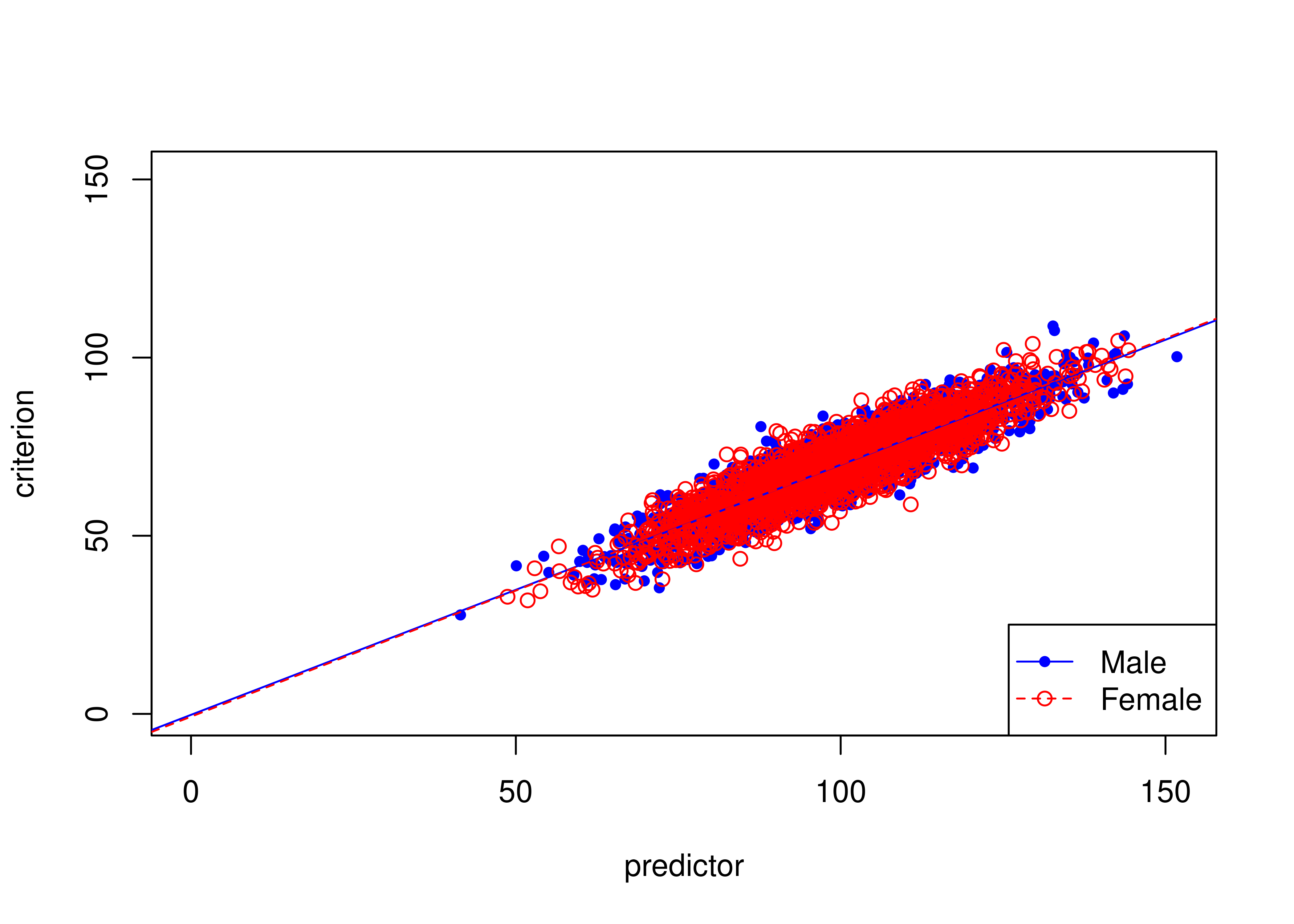
Figure 16.22: Example of Unbiased Prediction (No Differences in Intercepts or Slopes Between Males and Females).
16.8.2 Example of intercept bias
Figure 16.23 depicts an example of a biased test due to intercept bias.
There are differences in the intercepts of the regression lines (of predictor predicting criterion2) between males and females: males have a higher intercept than females.
That is, the same score on the predictor results in higher predictions for males than females.
Call:
lm(formula = criterion2 ~ predictor + group + predictor:group,
    data = mydataBias)

Residuals:
     Min       1Q   Median       3Q      Max
-18.6853  -3.4153  -0.0385   3.3979  18.0864

Coefficients:
                        Estimate Std. Error t value Pr(>|t|)
(Intercept)            10.054048   0.760084  13.228   <2e-16 ***
predictor               0.697987   0.007499  93.075   <2e-16 ***
groupfemale           -10.288893   1.074168  -9.578   <2e-16 ***
predictor:groupfemale   0.004748   0.010625   0.447    0.655
---
Signif. codes:  0 '***' 0.001 '**' 0.01 '*' 0.05 '.' 0.1 ' ' 1

Residual standard error: 5.037 on 3913 degrees of freedom
  (83 observations deleted due to missingness)
Multiple R-squared:  0.8452,    Adjusted R-squared:  0.8451
F-statistic:  7124 on 3 and 3913 DF,  p-value: < 2.2e-16
Code
plot(
  criterion2 ~ predictor,
  data = mydataBias,
  xlim = c(
    0,
    max(c(
      mydataBias$criterion2,
      mydataBias$predictor), na.rm = TRUE)),
  ylim = c(
    0,
    max(c(
      mydataBias$criterion2,
      mydataBias$predictor),
      na.rm = TRUE)),
  type = "n",
  xlab = "predictor",
  ylab = "criterion")
points(
  mydataBias$predictor[which(mydataBias$group == "male")],
  mydataBias$criterion2[which(mydataBias$group == "male")],
  pch = 20,
  col = "blue")
points(
  mydataBias$predictor[which(mydataBias$group == "female")],
  mydataBias$criterion2[which(mydataBias$group == "female")],
  pch = 1,
  col = "red")
abline(lm(
  criterion2 ~ predictor,
  data = mydataBias[which(mydataBias$group == "male"),]),
  lty = 1,
  col = "blue")
abline(lm(
  criterion2 ~ predictor,
  data = mydataBias[which(mydataBias$group == "female"),]),
  lty = 2,
  col = "red")
legend(
  "bottomright",
  c("Male","Female"),
  lty = c(1,2),
  pch = c(20,1),
  col = c("blue","red"))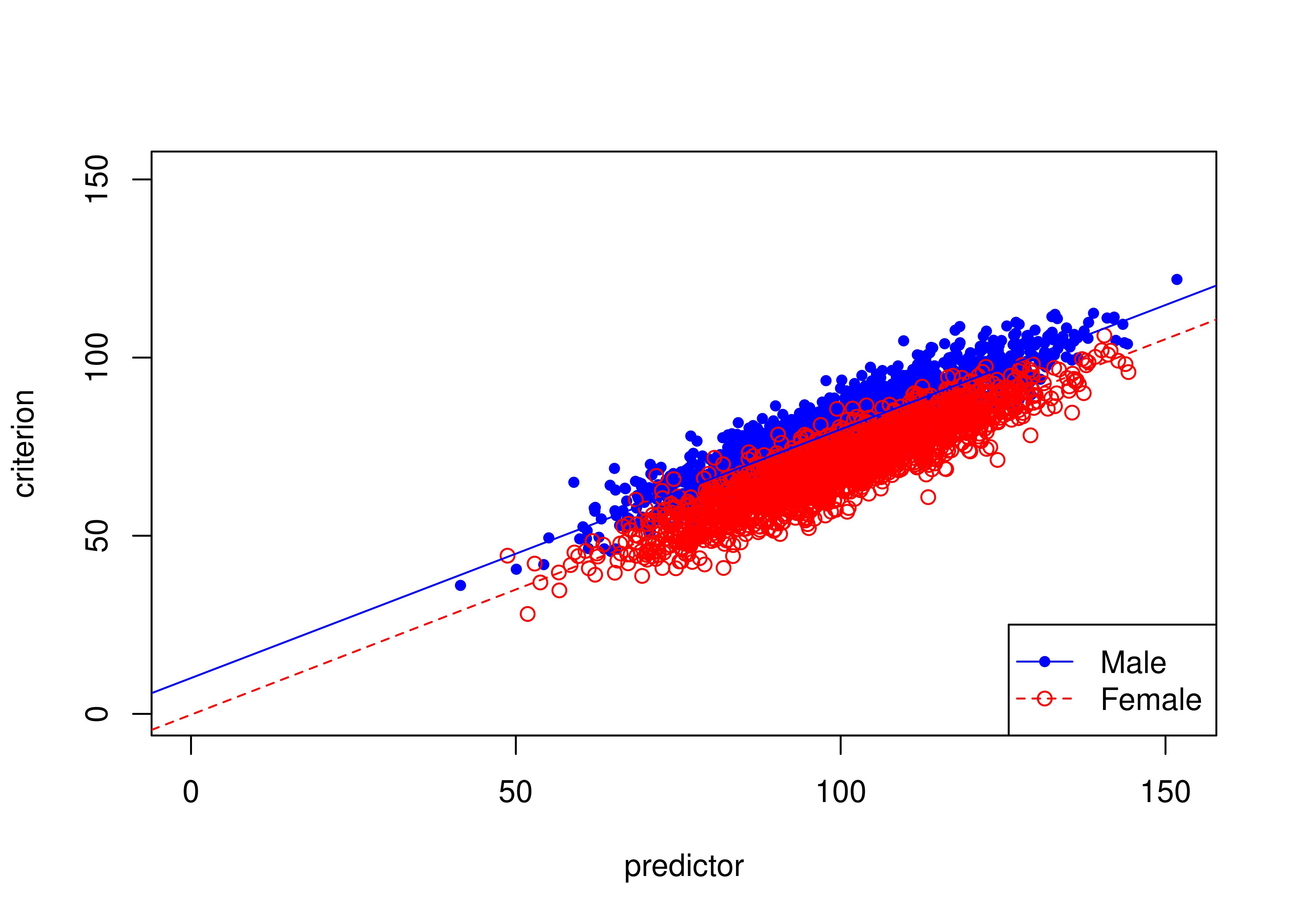
Figure 16.23: Example of Intercept Bias in Prediction (Different Intercepts Between Males and Females).
16.8.3 Example of slope bias
Figure 16.24 depicts an example of a biased test due to slope bias.
There are differences in the slopes of the regression lines (of predictor predicting criterion3) between males and females: males have a higher slope than females.
That is, scores have stronger predictive validity for males than females.
Call:
lm(formula = criterion3 ~ predictor + group + predictor:group,
    data = mydataBias)

Residuals:
     Min       1Q   Median       3Q      Max
-18.3183  -3.3715   0.0256   3.3844  19.3484

Coefficients:
                       Estimate Std. Error t value Pr(>|t|)
(Intercept)           -1.041940   0.757914  -1.375    0.169
predictor              0.708670   0.007475  94.804   <2e-16 ***
groupfemale            1.478534   1.074064   1.377    0.169
predictor:groupfemale -0.413233   0.010621 -38.907   <2e-16 ***
---
Signif. codes:  0 '***' 0.001 '**' 0.01 '*' 0.05 '.' 0.1 ' ' 1

Residual standard error: 5.031 on 3927 degrees of freedom
  (69 observations deleted due to missingness)
Multiple R-squared:  0.9489,    Adjusted R-squared:  0.9489
F-statistic: 2.432e+04 on 3 and 3927 DF,  p-value: < 2.2e-16
Code
plot(
  criterion3 ~ predictor,
  data = mydataBias,
  xlim = c(
    0,
    max(c(
      mydataBias$criterion3,
      mydataBias$predictor),
      na.rm = TRUE)),
  ylim = c(
    0,
    max(c(
      mydataBias$criterion3,
      mydataBias$predictor),
      na.rm = TRUE)),
  type = "n",
  xlab = "predictor",
  ylab = "criterion")
points(
  mydataBias$predictor[which(mydataBias$group == "male")],
  mydataBias$criterion3[which(mydataBias$group == "male")],
  pch = 20,
  col = "blue")
points(
  mydataBias$predictor[which(mydataBias$group == "female")],
  mydataBias$criterion3[which(mydataBias$group == "female")],
  pch = 1,
  col = "red")
abline(lm(
  criterion3 ~ predictor,
  data = mydataBias[which(mydataBias$group == "male"),]),
  lty = 1,
  col = "blue")
abline(lm(
  criterion3 ~ predictor,
  data = mydataBias[which(mydataBias$group == "female"),]),
  lty = 2,
  col = "red")
legend(
  "bottomright",
  c("Male","Female"),
  lty = c(1,2),
  pch = c(20,1),
  col = c("blue","red"))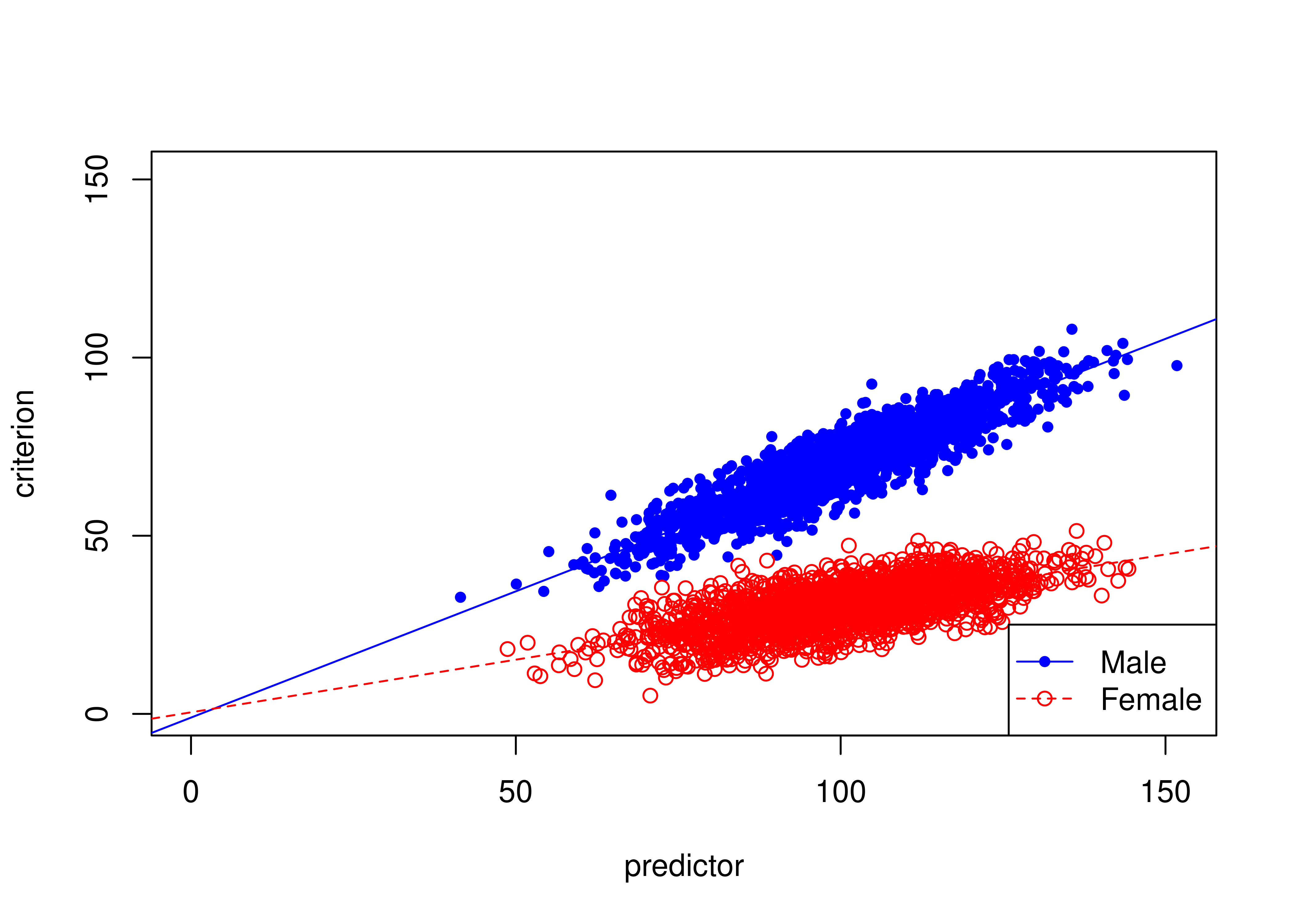
Figure 16.24: Example of Slope Bias in Prediction (Different Slopes Between Males And Females).
16.8.4 Example of intercept and slope bias
Figure 16.25 depicts an example of a biased test due to intercept and slope bias.
There are differences in the intercepts and slopes of the regression lines (of predictor predicting criterion4) between males and females: males have a higher slope than females.
That is, scores have stronger predictive validity for males than females.
Females have a higher intercept than males.
That is, at lower scores, the same score on the predictor results in higher predictions for females than males; at higher scores on the predictor, the same score results in higher predictions for males than females.
Call:
lm(formula = criterion4 ~ predictor + group + predictor:group,
    data = mydataBias)

Residuals:
     Min       1Q   Median       3Q      Max
-18.2805  -3.4400   0.0269   3.3199  17.8824

Coefficients:
                       Estimate Std. Error t value Pr(>|t|)
(Intercept)           -0.276228   0.767080   -0.36    0.719
predictor              0.702178   0.007565   92.81   <2e-16 ***
groupfemale           29.156167   1.086254   26.84   <2e-16 ***
predictor:groupfemale -0.392016   0.010743  -36.49   <2e-16 ***
---
Signif. codes:  0 '***' 0.001 '**' 0.01 '*' 0.05 '.' 0.1 ' ' 1

Residual standard error: 5.099 on 3930 degrees of freedom
  (66 observations deleted due to missingness)
Multiple R-squared:  0.7843,    Adjusted R-squared:  0.7842
F-statistic:  4764 on 3 and 3930 DF,  p-value: < 2.2e-16
Code
plot(
  criterion4 ~ predictor,
  data = mydataBias,
  xlim = c(
    0,
    max(c(
      mydataBias$criterion4,
      mydataBias$predictor),
      na.rm = TRUE)),
  ylim = c(
    0,
    max(c(
      mydataBias$criterion4,
      mydataBias$predictor),
      na.rm = TRUE)),
  type = "n",
  xlab = "predictor",
  ylab = "criterion")
points(
  mydataBias$predictor[which(mydataBias$group == "male")],
  mydataBias$criterion4[which(mydataBias$group == "male")],
  pch = 20,
  col = "blue")
points(
  mydataBias$predictor[which(mydataBias$group == "female")],
  mydataBias$criterion4[which(mydataBias$group == "female")],
  pch = 1,
  col = "red")
abline(lm(
  criterion4 ~ predictor,
  data = mydataBias[which(mydataBias$group == "male"),]),
  lty = 1,
  col = "blue")
abline(lm(
  criterion4 ~ predictor,
  data = mydataBias[which(mydataBias$group == "female"),]),
  lty = 2,
  col = "red")
legend(
  "bottomright",
  c("Male","Female"),
  lty = c(1,2),
  pch = c(20,1),
  col = c("blue","red"))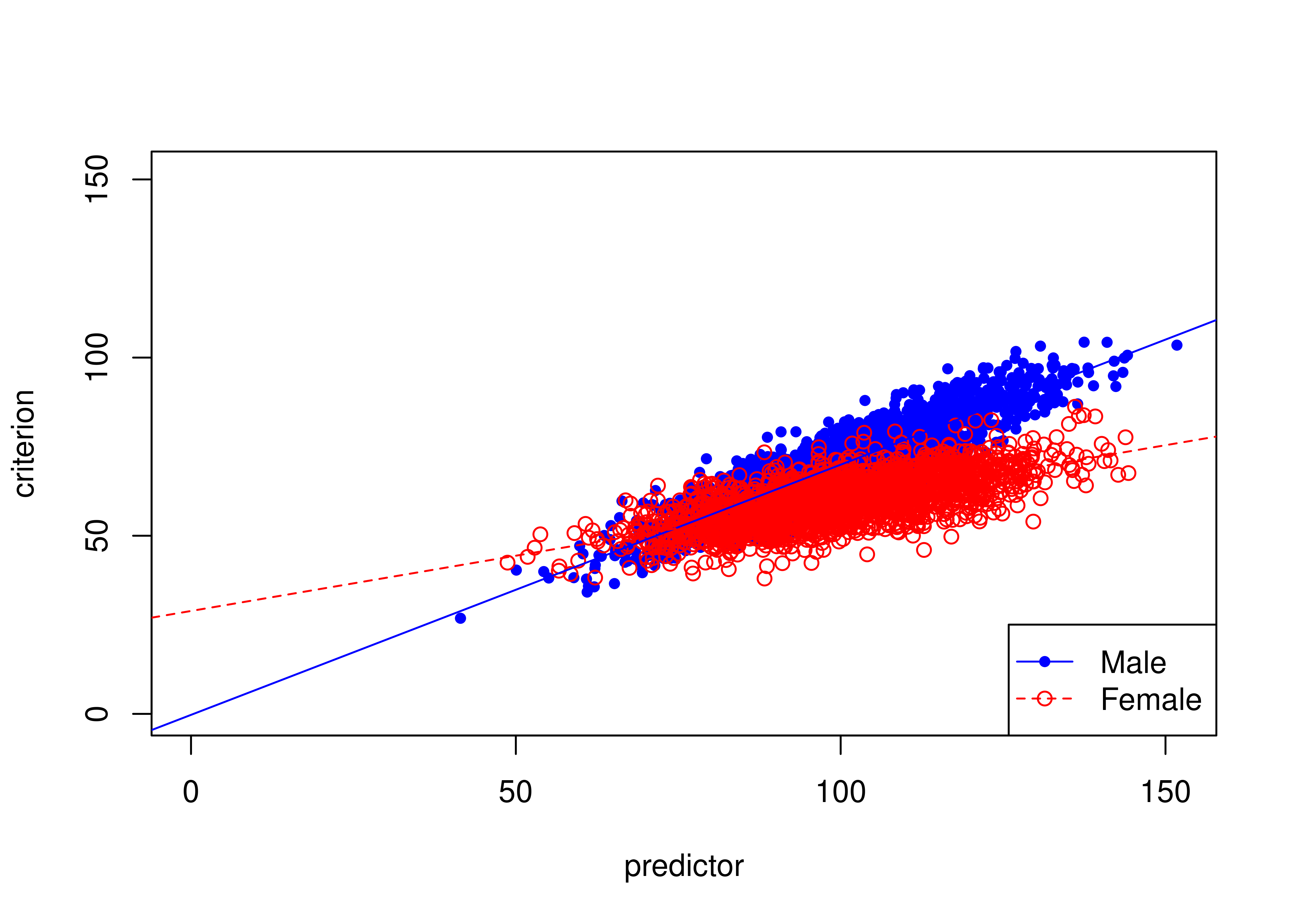
Figure 16.25: Example of Intercept And Slope Bias in Prediction (Different Intercepts and Slopes Between Males and Females).
16.8.5 Example of different measurement reliability/error across groups
In the example depicted in Figure 16.26, there are differences in the measurement reliability/error on the criterion between males and females: males’ scores have a lower reliability (higher measurement error) on the criterion than females’ scores. That is, we are more confident about a female’s level on the criterion given a particular score on the predictor than we are about a male’s level on the criterion given a particular score on the predictor.
Call:
lm(formula = criterion5 ~ predictor + group + predictor:group,
    data = mydataBias)

Residuals:
     Min       1Q   Median       3Q      Max
-109.295   -7.065    0.077    6.836  108.428

Coefficients:
                      Estimate Std. Error t value Pr(>|t|)
(Intercept)           -9.28386    3.32617  -2.791  0.00528 **
predictor              0.79172    0.03280  24.136  < 2e-16 ***
groupfemale            9.12452    4.70470   1.939  0.05252 .
predictor:groupfemale -0.09083    0.04654  -1.952  0.05102 .
---
Signif. codes:  0 '***' 0.001 '**' 0.01 '*' 0.05 '.' 0.1 ' ' 1

Residual standard error: 22.03 on 3920 degrees of freedom
  (76 observations deleted due to missingness)
Multiple R-squared:  0.2087,    Adjusted R-squared:  0.2081
F-statistic: 344.6 on 3 and 3920 DF,  p-value: < 2.2e-16
Code
plot(
  criterion5 ~ predictor,
  data = mydataBias,
  xlim = c(
    0,
    max(c(mydataBias$criterion5,
          mydataBias$predictor),
        na.rm = TRUE)),
  ylim = c(
    0,
    max(c(
      mydataBias$criterion5,
      mydataBias$predictor),
      na.rm = TRUE)),
  type = "n",
  xlab = "predictor",
  ylab = "criterion")
points(
  mydataBias$predictor[which(mydataBias$group == "male")],
  mydataBias$criterion5[which(mydataBias$group == "male")],
  pch = 20,
  col = "blue")
points(mydataBias$predictor[which(mydataBias$group == "female")],
       mydataBias$criterion5[which(mydataBias$group == "female")],
       pch = 1,
       col = "red")
abline(lm(criterion5 ~ predictor,
          data = mydataBias[which(mydataBias$group == "male"),]),
       lty = 1,
       col = "blue")
abline(lm(criterion5 ~ predictor,
          data = mydataBias[which(mydataBias$group == "female"),]),
       lty = 2,
       col = "red")
legend(
  "bottomright",
  c("Male","Female"),
  lty = c(1,2),
  pch = c(20,1),
  col = c("blue","red"))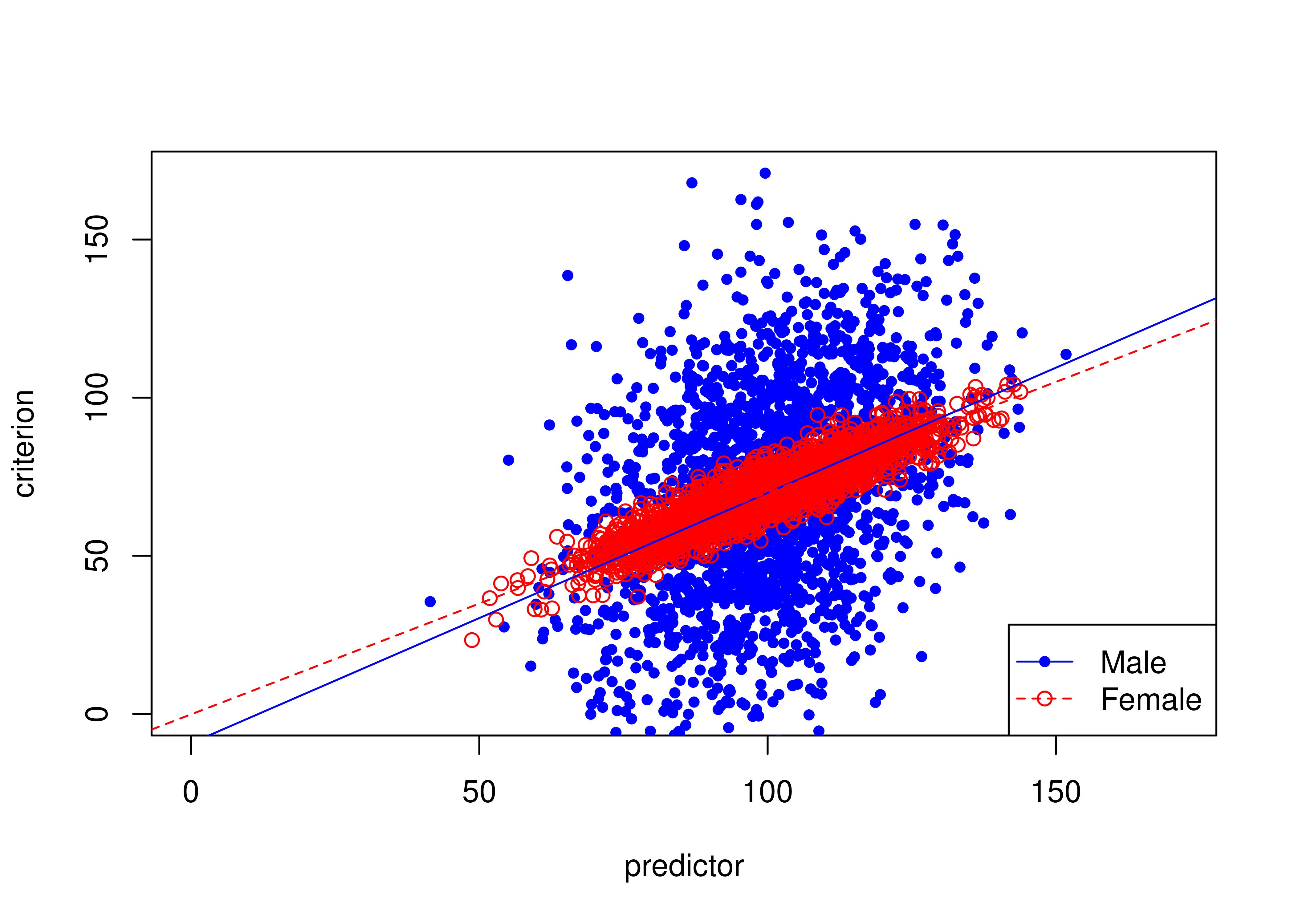
Figure 16.26: Example of Different Measurement Reliability/Error Across Groups.
16.9 Differential Item Functioning (DIF)
Differential item functioning (DIF) indicates that one or more items functions differently across groups. That is, one or more of the item parameters for an item differs across groups. For instance, the severity or discrimination of an item could be higher in one group compared to another group. If an item functions differently across groups, it can lead to biased scores for particular groups. Thus, when observing group differences in level on the measure or group differences in the measure’s association with other measures, it is unclear whether the observed group differences reflect true group differences or differences in the functioning of the measure across groups.
For instance, consider an item such as “disobedience to authority”, which is thought to reflect externalizing behavior in childhood. However, in adulthood, disobedience to authority could reflect prosocial functions, such as protesting against societally unjust actions, and may show weaker construct validity with respect to externalizing problems, as operationalized by a weaker discrimination coefficient in adulthood than in childhood. Tests of differential item functioning are equivalent to tests of measurement invariance.
Approaches to addressing DIF are described in Section 16.5.1. If we identify that an item shows non-negligible DIF, we have three primary options (described above): (1) drop the item for both groups, (2) drop the item for one group but keep it for the other group, or (3) freely estimate the parameters (discrimination and difficulty) for the item across groups.
Tests of DIF were conducted using the mirt package (Chalmers, 2020).
16.9.1 Item Descriptive Statistics
Code
$female
$female$overall
 N.complete    N mean_total.score sd_total.score ave.r  sd.r alpha SEM.alpha
       1620 5641            2.554          2.132 0.255 0.083 0.681     1.203

$female$itemstats
                      N K  mean    sd total.r total.r_if_rm alpha_if_rm
bpi_antisocialT1_1 1928 3 0.538 0.587   0.665         0.455       0.626
bpi_antisocialT1_2 1925 3 0.278 0.510   0.647         0.465       0.624
bpi_antisocialT1_3 1925 3 0.456 0.654   0.618         0.359       0.657
bpi_antisocialT1_4 1933 3 0.113 0.355   0.514         0.371       0.654
bpi_antisocialT1_5 1649 3 0.186 0.431   0.587         0.429       0.637
bpi_antisocialT1_6 1658 3 0.103 0.345   0.571         0.446       0.643
bpi_antisocialT1_7 1944 3 0.834 0.639   0.563         0.294       0.683

$female$proportions
                       0     1     2  <NA>
bpi_antisocialT1_1 0.174 0.151 0.016 0.658
bpi_antisocialT1_2 0.257 0.075 0.010 0.659
bpi_antisocialT1_3 0.216 0.094 0.031 0.659
bpi_antisocialT1_4 0.308 0.030 0.004 0.657
bpi_antisocialT1_5 0.243 0.044 0.005 0.708
bpi_antisocialT1_6 0.268 0.023 0.004 0.706
bpi_antisocialT1_7 0.104 0.194 0.046 0.655

$female$total.score_frequency
       0   1   2   3   4  5  6  7  8  9 10 11 12 13
Freq 217 364 349 283 166 91 67 38 12 10 11  4  4  4

$female$total.score_means
                          0        1        2
bpi_antisocialT1_1 1.354919 3.339237 7.216867
bpi_antisocialT1_2 1.846343 4.173789 8.192308
bpi_antisocialT1_3 1.593417 3.846682 5.406667
bpi_antisocialT1_4 2.204952 5.090278 9.045455
bpi_antisocialT1_5 2.010386 4.946721 7.892857
bpi_antisocialT1_6 2.189959 5.701613 9.227273
bpi_antisocialT1_7 1.004357 2.778970 4.746725

$female$total.score_sds
                          0        1        2
bpi_antisocialT1_1 1.262270 1.668474 2.763209
bpi_antisocialT1_2 1.480206 1.809814 2.664498
bpi_antisocialT1_3 1.329902 1.837884 2.783211
bpi_antisocialT1_4 1.743521 2.280698 2.802673
bpi_antisocialT1_5 1.566126 2.196431 3.258485
bpi_antisocialT1_6 1.684322 2.215906 2.844072
bpi_antisocialT1_7 1.232733 1.798814 2.475591


$male
$male$overall
 N.complete    N mean_total.score sd_total.score ave.r  sd.r alpha SEM.alpha
       1645 5891             3.16          2.385 0.266 0.081 0.703       1.3

$male$itemstats
                      N K  mean    sd total.r total.r_if_rm alpha_if_rm
bpi_antisocialT1_1 1948 3 0.615 0.585   0.639         0.451       0.660
bpi_antisocialT1_2 1947 3 0.372 0.559   0.664         0.494       0.650
bpi_antisocialT1_3 1949 3 0.520 0.668   0.593         0.358       0.692
bpi_antisocialT1_4 1948 3 0.233 0.486   0.594         0.434       0.666
bpi_antisocialT1_5 1676 3 0.367 0.547   0.629         0.457       0.662
bpi_antisocialT1_6 1688 3 0.177 0.446   0.549         0.398       0.675
bpi_antisocialT1_7 1962 3 0.834 0.646   0.587         0.360       0.687

$male$proportions
                       0     1     2  <NA>
bpi_antisocialT1_1 0.145 0.168 0.017 0.669
bpi_antisocialT1_2 0.220 0.097 0.013 0.669
bpi_antisocialT1_3 0.191 0.107 0.033 0.669
bpi_antisocialT1_4 0.263 0.058 0.010 0.669
bpi_antisocialT1_5 0.190 0.085 0.010 0.715
bpi_antisocialT1_6 0.243 0.035 0.008 0.713
bpi_antisocialT1_7 0.102 0.185 0.046 0.667

$male$total.score_frequency
       0   1   2   3   4   5   6  7  8  9 10 11 12 13 14
Freq 163 294 310 259 208 144 104 74 40 25  9  7  5  1  2

$male$total.score_means
                          0        1        2
bpi_antisocialT1_1 1.622478 3.944056 7.397849
bpi_antisocialT1_2 2.134191 4.767821 8.106061
bpi_antisocialT1_3 2.016754 4.400763 5.819277
bpi_antisocialT1_4 2.484091 5.539286 8.177778
bpi_antisocialT1_5 2.174111 4.817073 7.910714
bpi_antisocialT1_6 2.616762 5.810680 8.093023
bpi_antisocialT1_7 1.412500 3.375679 5.782787

$male$total.score_sds
                          0        1        2
bpi_antisocialT1_1 1.515237 1.982218 2.454542
bpi_antisocialT1_2 1.678482 1.955386 2.437709
bpi_antisocialT1_3 1.654589 2.069463 2.774973
bpi_antisocialT1_4 1.845772 2.119687 2.534210
bpi_antisocialT1_5 1.709715 2.047072 2.725481
bpi_antisocialT1_6 1.911288 2.181537 2.982600
bpi_antisocialT1_7 1.522500 1.906515 2.652344
16.9.2 Unconstrained Model
16.9.2.2 Model Summary
Items that appear to differ:
- items 5 and 6 are more discriminating (\(a\) parameter) among females than males
- item 4 has higher difficulty/severity (\(b_1\) and \(b_2\) parameters) among males than females
----------
GROUP: female
        F1    h2
[1,] 0.698 0.487
[2,] 0.706 0.499
[3,] 0.532 0.283
[4,] 0.683 0.466
[5,] 0.763 0.582
[6,] 0.838 0.702
[7,] 0.429 0.184

SS loadings:  3.202
Proportion Var:  0.457

Factor correlations:

   F1
F1  1

----------
GROUP: male
        F1    h2
[1,] 0.663 0.440
[2,] 0.736 0.542
[3,] 0.531 0.282
[4,] 0.713 0.508
[5,] 0.691 0.477
[6,] 0.702 0.492
[7,] 0.507 0.257

SS loadings:  2.999
Proportion Var:  0.428

Factor correlations:

   F1
F1 1$female
$items
a b1 b2
bpi_antisocialT1_1 1.657 0.029 2.451
bpi_antisocialT1_2 1.697 0.953 2.763
bpi_antisocialT1_3 1.069 0.650 2.585
bpi_antisocialT1_4 1.590 1.895 3.465
bpi_antisocialT1_5 2.008 1.281 2.936
bpi_antisocialT1_6 2.614 1.625 2.770
bpi_antisocialT1_7 0.807 -1.184 2.583
$means
F1
0
$cov
F1
F1 1
$male
$items
a b1 b2
bpi_antisocialT1_1 1.507 -0.238 2.505
bpi_antisocialT1_2 1.853 0.582 2.455
bpi_antisocialT1_3 1.067 0.384 2.480
bpi_antisocialT1_4 1.729 1.165 2.765
bpi_antisocialT1_5 1.625 0.635 2.757
bpi_antisocialT1_6 1.677 1.494 2.873
bpi_antisocialT1_7 1.002 -0.986 2.143
$means
F1
0
$cov
F1
F1 116.9.3 Constrained Model
Constrain item parameters to be equal across groups (to use as baseline model for identifying DIF).
16.9.3.1 Fit Model
Code
constrainedModel <- multipleGroup(
  data = cnlsy[,c(
    "bpi_antisocialT1_1","bpi_antisocialT1_2","bpi_antisocialT1_3",
    "bpi_antisocialT1_4","bpi_antisocialT1_5","bpi_antisocialT1_6",
    "bpi_antisocialT1_7")],
  model = 1,
  group = cnlsy$sex,
  invariance = c(c(
    "bpi_antisocialT1_1","bpi_antisocialT1_2","bpi_antisocialT1_3",
    "bpi_antisocialT1_4","bpi_antisocialT1_5","bpi_antisocialT1_6",
    "bpi_antisocialT1_7"),
    "free_means", "free_var"),
  SE = TRUE)
16.9.3.2 Model Summary
----------
GROUP: female
        F1    h2
[1,] 0.657 0.431
[2,] 0.707 0.500
[3,] 0.512 0.262
[4,] 0.701 0.491
[5,] 0.733 0.538
[6,] 0.765 0.585
[7,] 0.440 0.193

SS loadings:  3
Proportion Var:  0.429

Factor correlations:

   F1
F1  1

----------
GROUP: male
        F1    h2
[1,] 0.672 0.452
[2,] 0.722 0.521
[3,] 0.527 0.278
[4,] 0.716 0.512
[5,] 0.747 0.559
[6,] 0.778 0.605
[7,] 0.455 0.207

SS loadings:  3.134
Proportion Var:  0.448

Factor correlations:

   F1
F1 1$female
$items
a b1 b2
bpi_antisocialT1_1 1.482 0.078 2.798
bpi_antisocialT1_2 1.701 0.973 2.892
bpi_antisocialT1_3 1.013 0.726 2.844
bpi_antisocialT1_4 1.673 1.688 3.278
bpi_antisocialT1_5 1.836 1.135 3.028
bpi_antisocialT1_6 2.020 1.782 3.048
bpi_antisocialT1_7 0.834 -0.967 2.697
$means
F1
0
$cov
F1
F1 1
$male
$items
a b1 b2
bpi_antisocialT1_1 1.482 0.078 2.798
bpi_antisocialT1_2 1.701 0.973 2.892
bpi_antisocialT1_3 1.013 0.726 2.844
bpi_antisocialT1_4 1.673 1.688 3.278
bpi_antisocialT1_5 1.836 1.135 3.028
bpi_antisocialT1_6 2.020 1.782 3.048
bpi_antisocialT1_7 0.834 -0.967 2.697
$means
F1
0.37
$cov
F1
F1 1.08816.9.4 Compare model fit of constrained model to unconstrained model
The constrained model and the unconstrained model are considered “nested” models. The constrained model is nested within the unconstrained model because the unconstrained model includes all of the terms of the constrained model along with additional terms. Model fit of nested models can be compared with a chi-square difference test.
The constrained model fits significantly worse than the unconstrained model, which suggests that item parameters differ between males and females.
16.9.5 Identify DIF by iteratively removing constraints from fully constrained model
One way to identify DIF is to iteratively remove constraints from a model in which all parameters are constrained to be the same across groups. Removing constraints allows individual items to have different item parameters across groups, to identify which items yield a significant improvement in model fit when allowing their discrimination and/or severity to differ across groups. Items 1, 3, 4, 5, 6, and 7 showed DIF in discrimination and/or severity, based on a significant chi-square difference test.
16.9.5.2 Items that differ in discrimination
Items 1, 3, 4, and 5 showed DIF in discrimination, based on a significant chi-square difference test.
Code
16.9.5.3 Items that differ in severity
Items 1, 3, 4, 5, and 7 showed DIF in difficulty/severity, based on a significant chi-square difference test.
Code
16.9.6 Identify DIF by iteratively adding constraints to unconstrained model
16.9.6.1 Items that differ in discrimination and/or severity
Another way to identify DIF is to iteratively add constraints to a model in which all parameters are allowed to differ across groups. Adding constraints forces individual items to have the same item parameters across groups, to identify which items yield a significant worsening in model fit when constraining their discrimination and/or severity to be the same across groups. Items 1, 2, 3, 4, 5, and 6 showed DIF in discrimination and/or severity, based on a significant chi-square difference test. The DIF in discrimination and/or severity is depicted in Figure 16.27.
Code
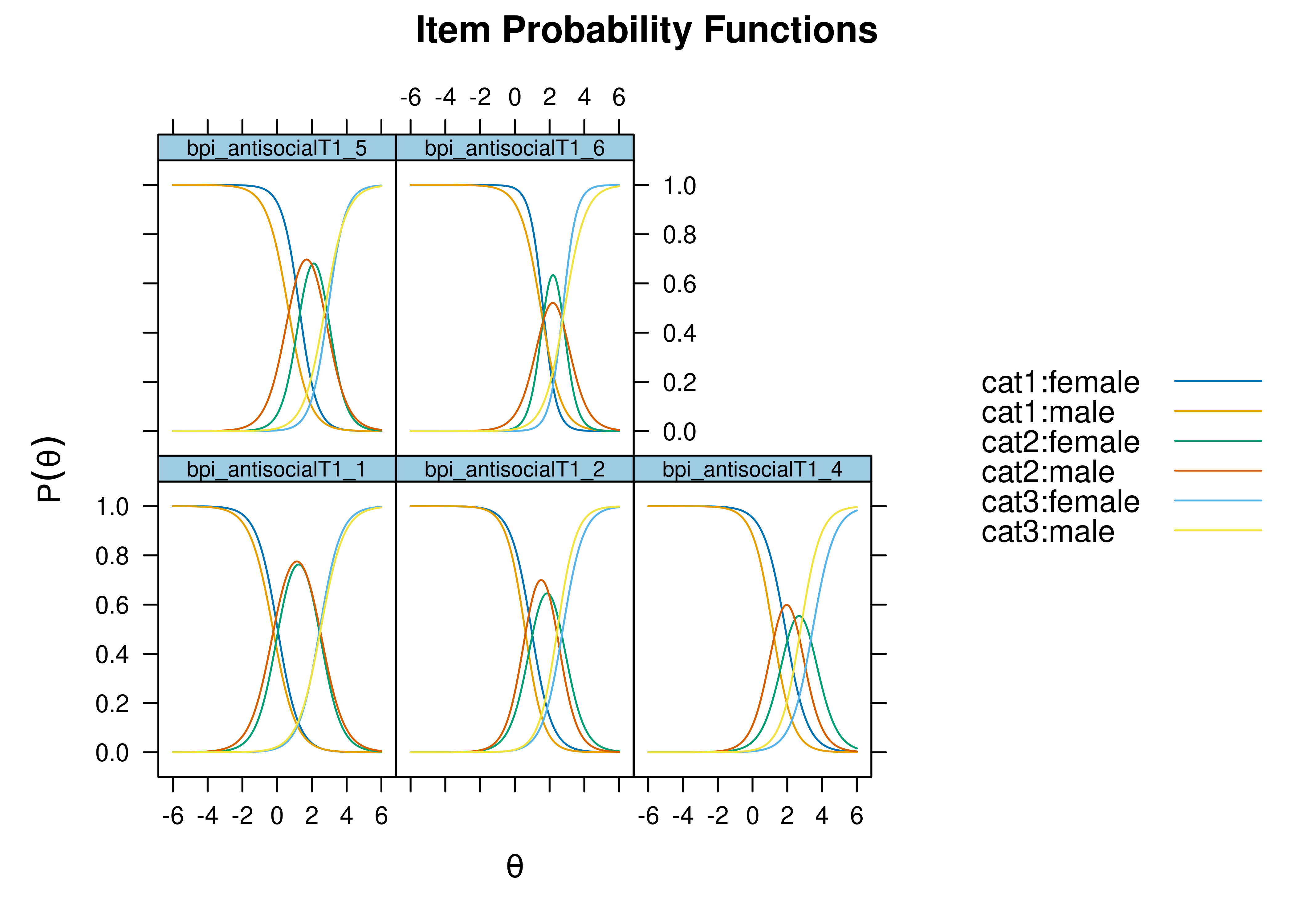
Figure 16.27: Item Probability Functions for Examining Differential Item Functioning in Terms of Discrimination and/or Severity.
16.9.6.2 Items that differ in discrimination
Items 6 and 7 showed DIF in discrimination, based on a significant chi-square difference test. The DIF in discrimination is depicted in Figure 16.28.
Code
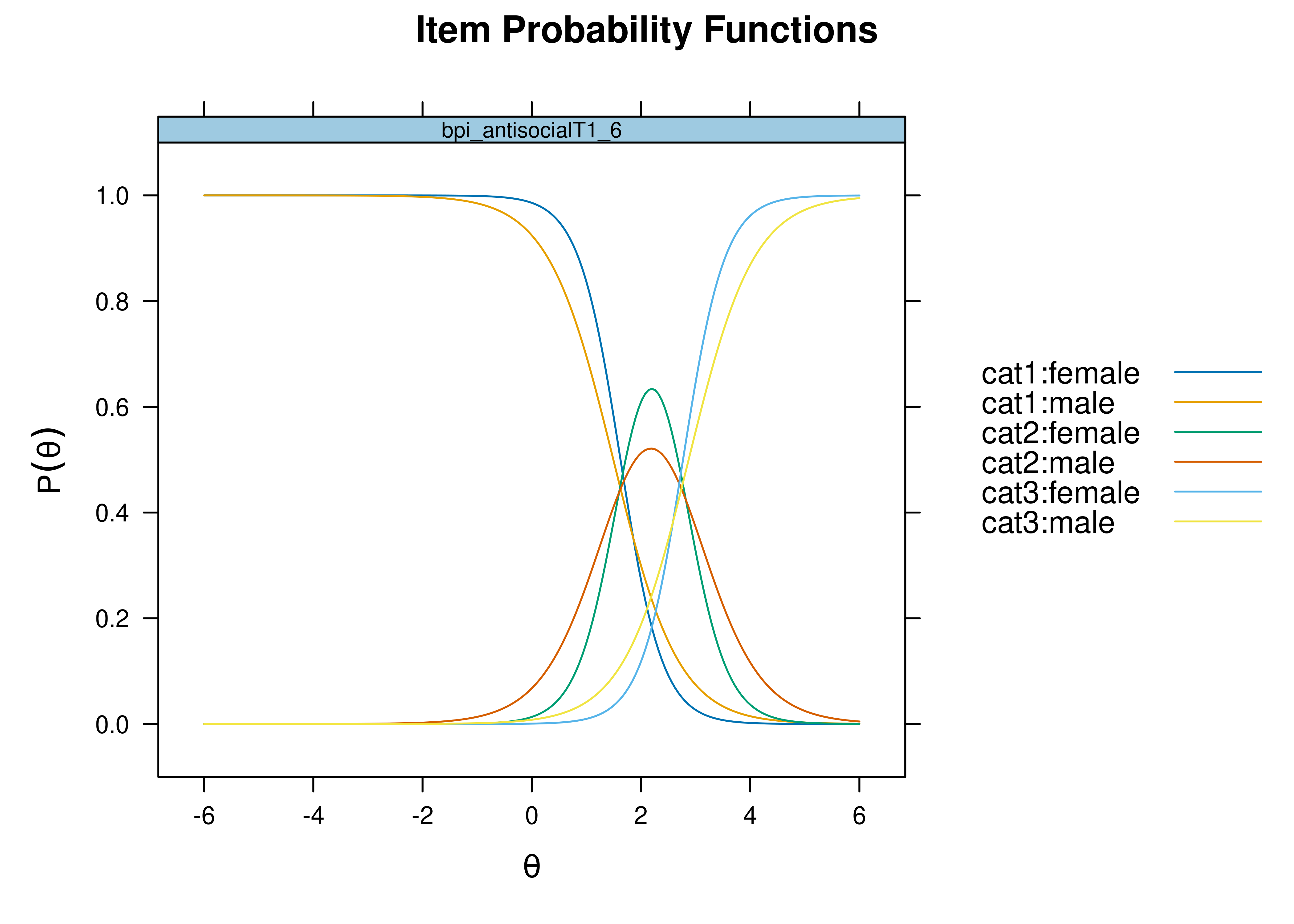
Figure 16.28: Item Probability Functions for Examining Differential Item Functioning in Terms of Discrimination.
16.9.6.3 Items that differ in severity
Items 1, 2, 3, 4, 5, and 6 showed DIF in difficulty/severity, based on a significant chi-square difference test. The DIF in difficulty/severity is depicted in Figure 16.29
Code
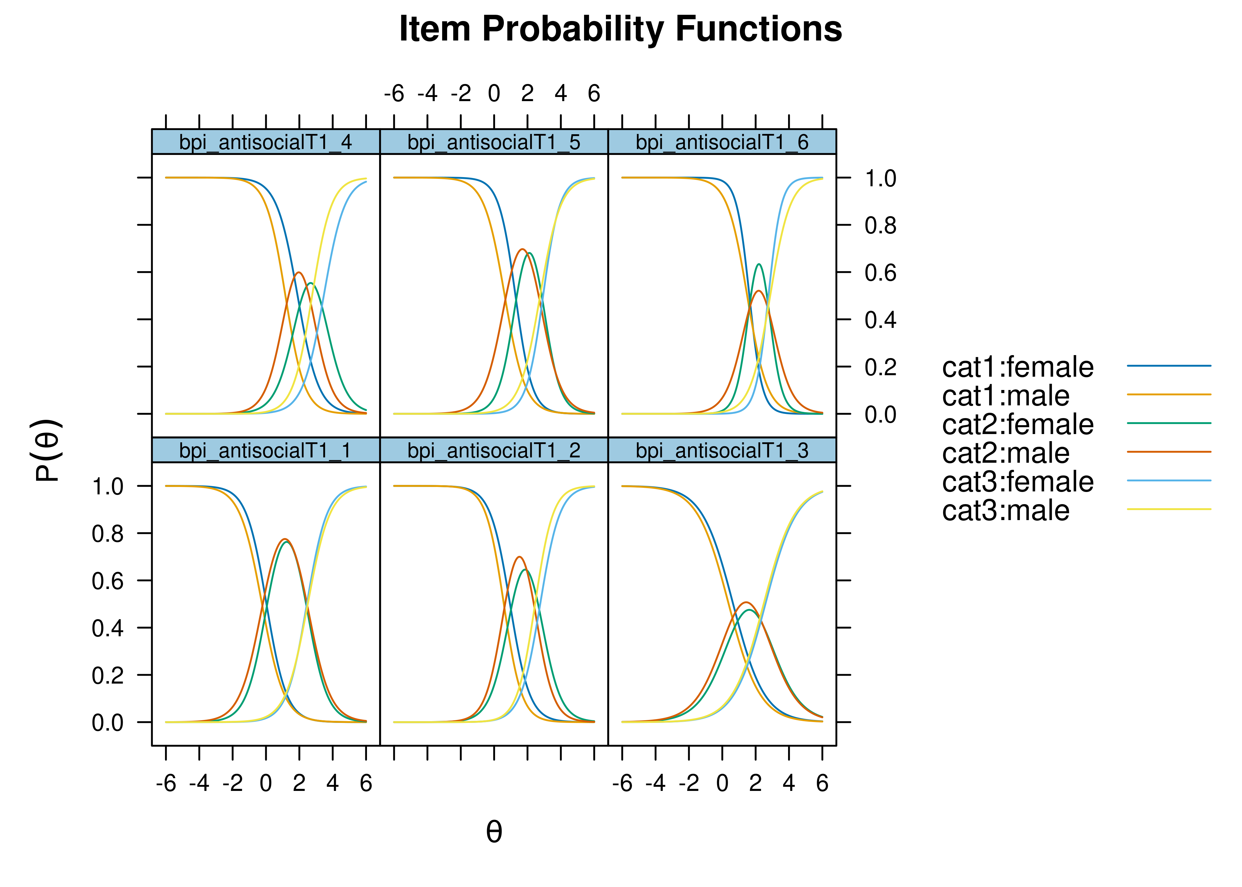
Figure 16.29: Item Probability Functions for Examining Differential Item Functioning in Terms of Severity.
16.9.7 Compute effect size of DIF
Effect size measures of DIF were computed based on expected scores (Meade, 2010) using the mirt package (Chalmers, 2020).
Some researchers recommend using a simulation-based procedure to examine the impact of DIF on screening accuracy (Gonzalez & Pelham, 2021).
16.9.7.1 Test-level DIF
In addition to consideration of differential test functioning, we can also consider whether the test as a whole (i.e., the collection of items) differs in its functioning by group—called differential test functioning. Differential test functioning is depicted in Figure 16.30. Estimates of differential test functioning are in Table ??.
In general, the measure showed greater difficulty for females than for males. That is, at a given construct level, males were more likely than females to endorse the items. Otherwise said, it takes a higher construct level for females to obtain the same score on the measure as males.
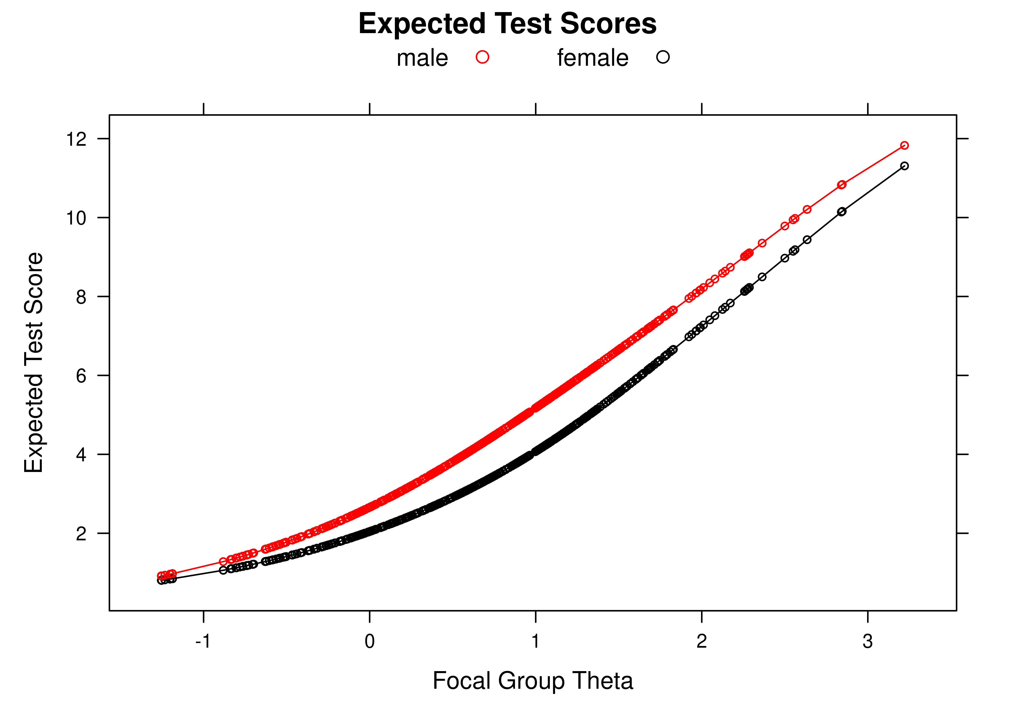
Figure 16.30: Differential Test Functioning by Sex.
16.9.7.2 Item-level DIF
Differential item functioning is depicted in Figure 16.31. Estimates of differential item functioning are in Table ??.
The measure-level differences in functioning appear to be largely driven by greater difficulty of items 4 and 5 for females than males. That is, at a given construct level, males were more likely than females to endorse items 4 and 5, in particular. Otherwise said, it takes a higher construct level for females than males to endorse items 4 and 5.
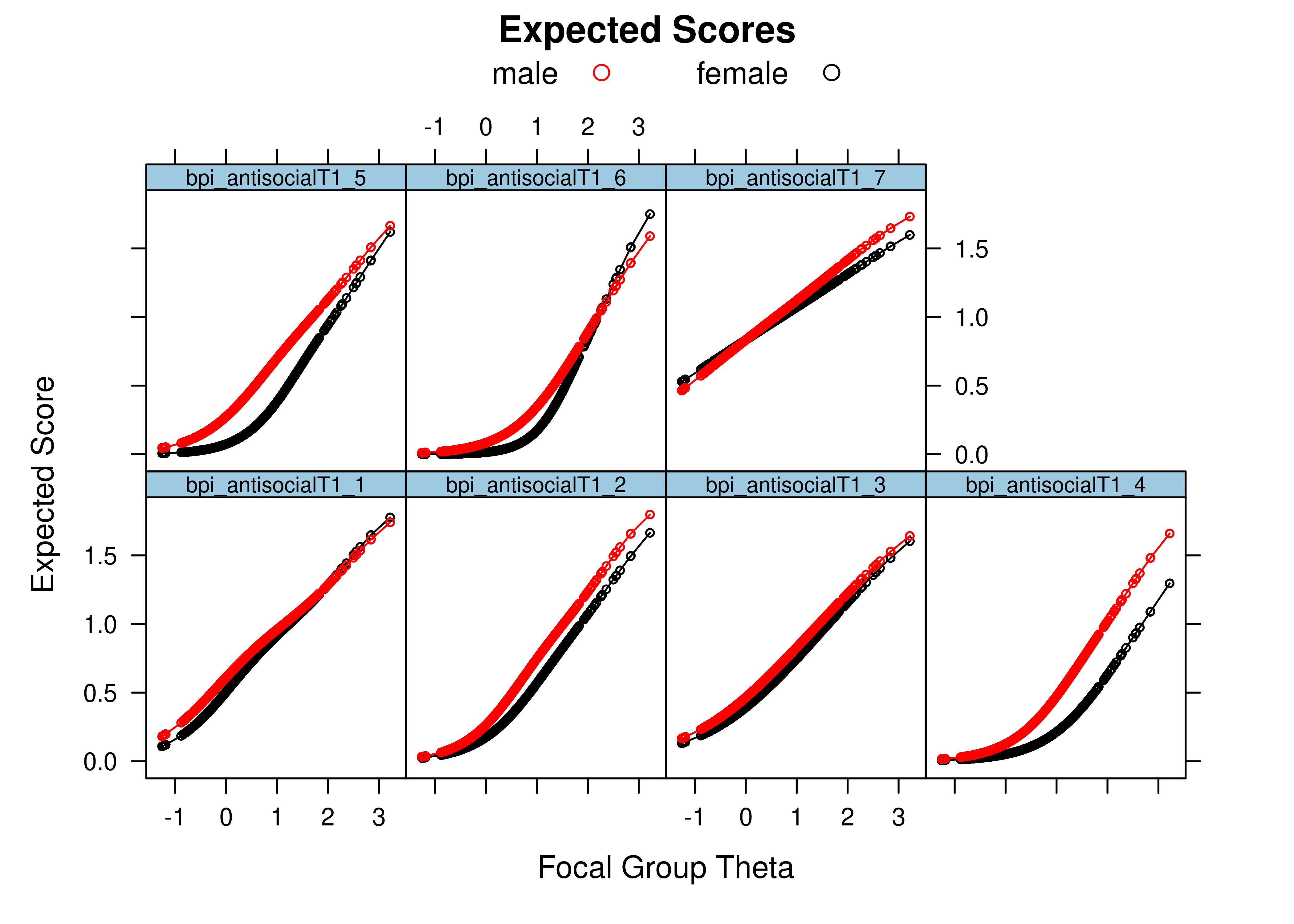
Figure 16.31: Differential Item Functioning by Sex.
16.9.8 Item plots
Plots of item response category characteristic curves by sex are in Figures 16.32–16.38 below.
Code
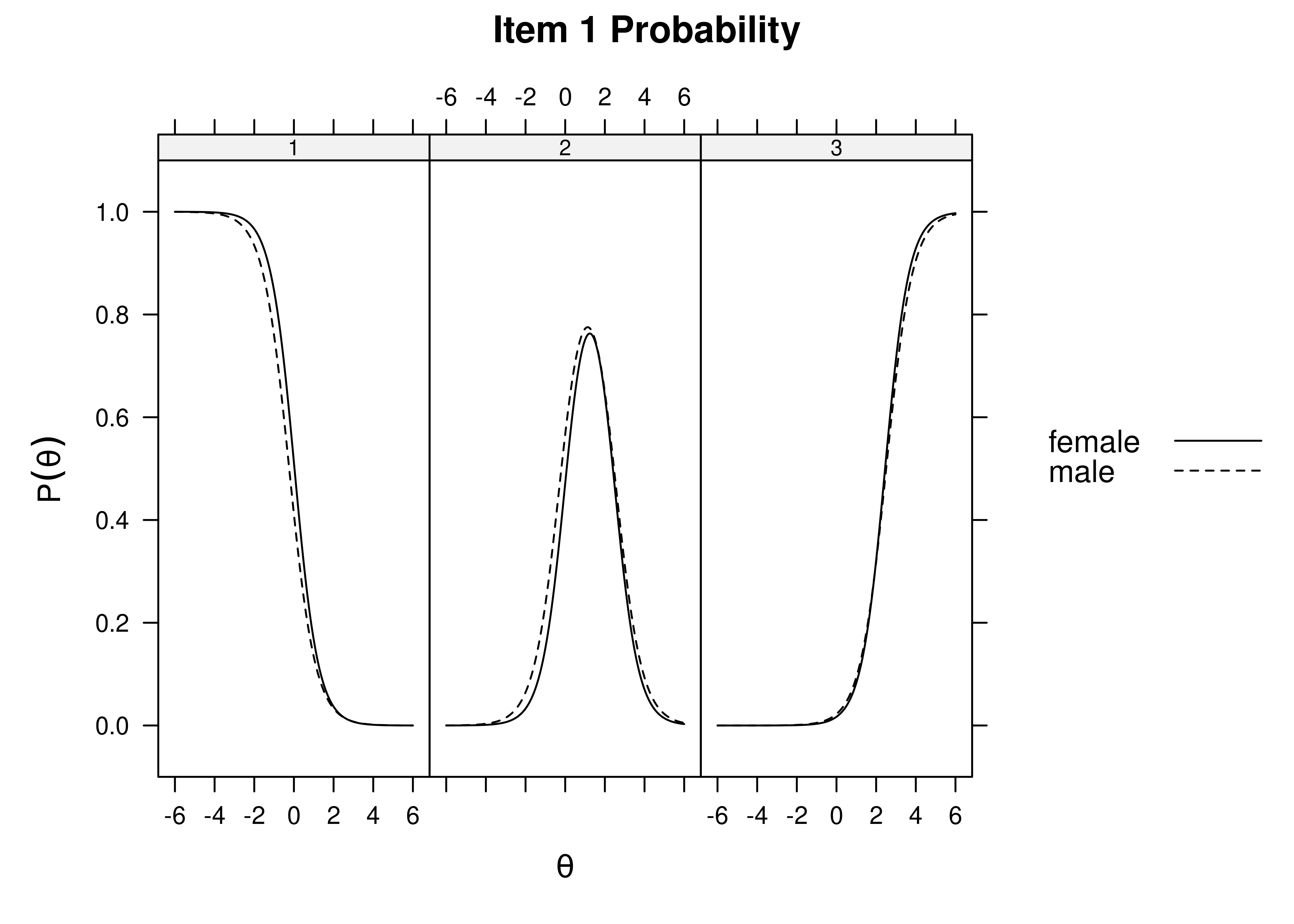
Figure 16.32: Item Response Category Characteristic Curves by Sex: Item 1.
Code

Figure 16.33: Item Response Category Characteristic Curves by Sex: Item 2.
Code
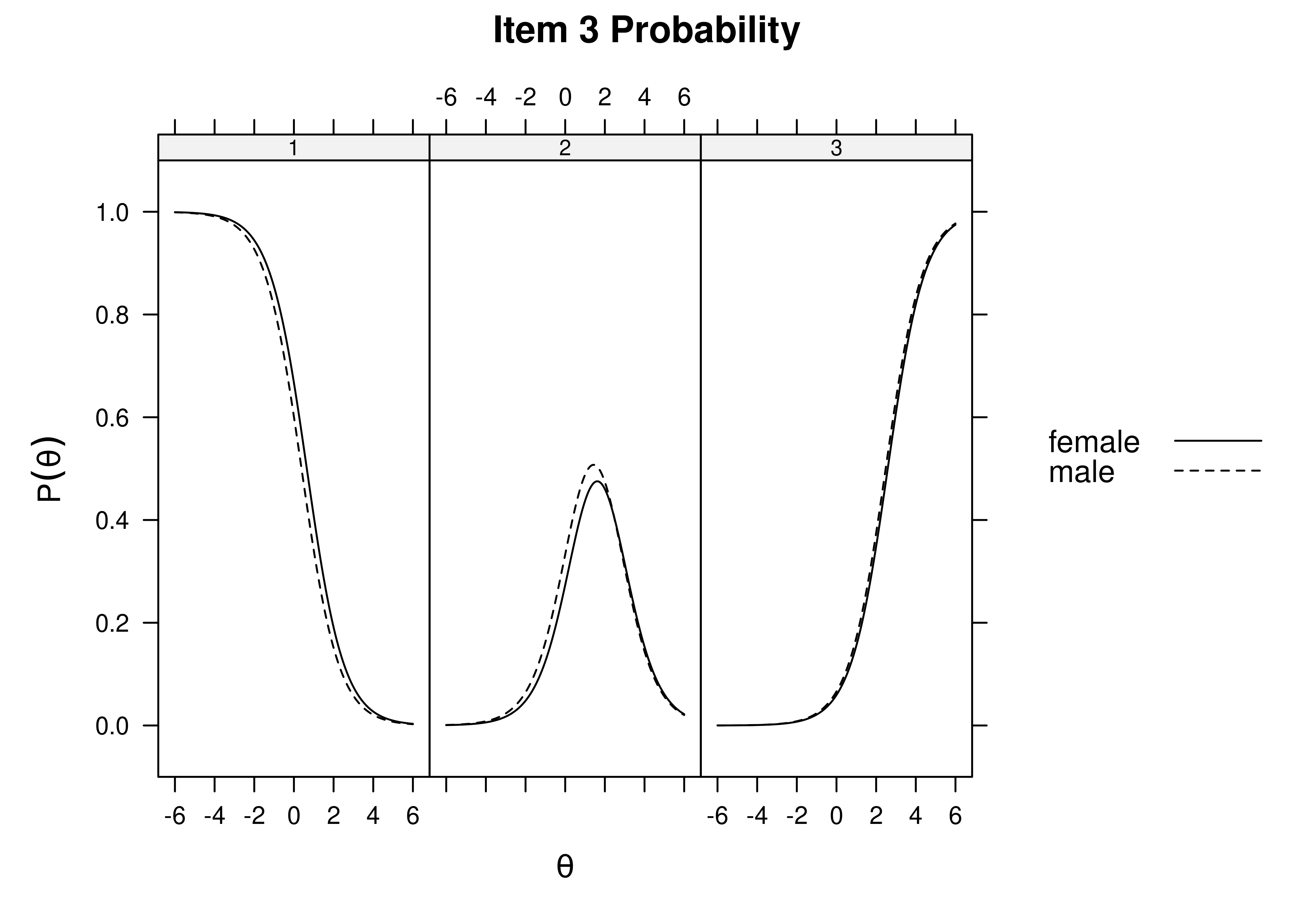
Figure 16.34: Item Response Category Characteristic Curves by Sex: Item 3.
Code
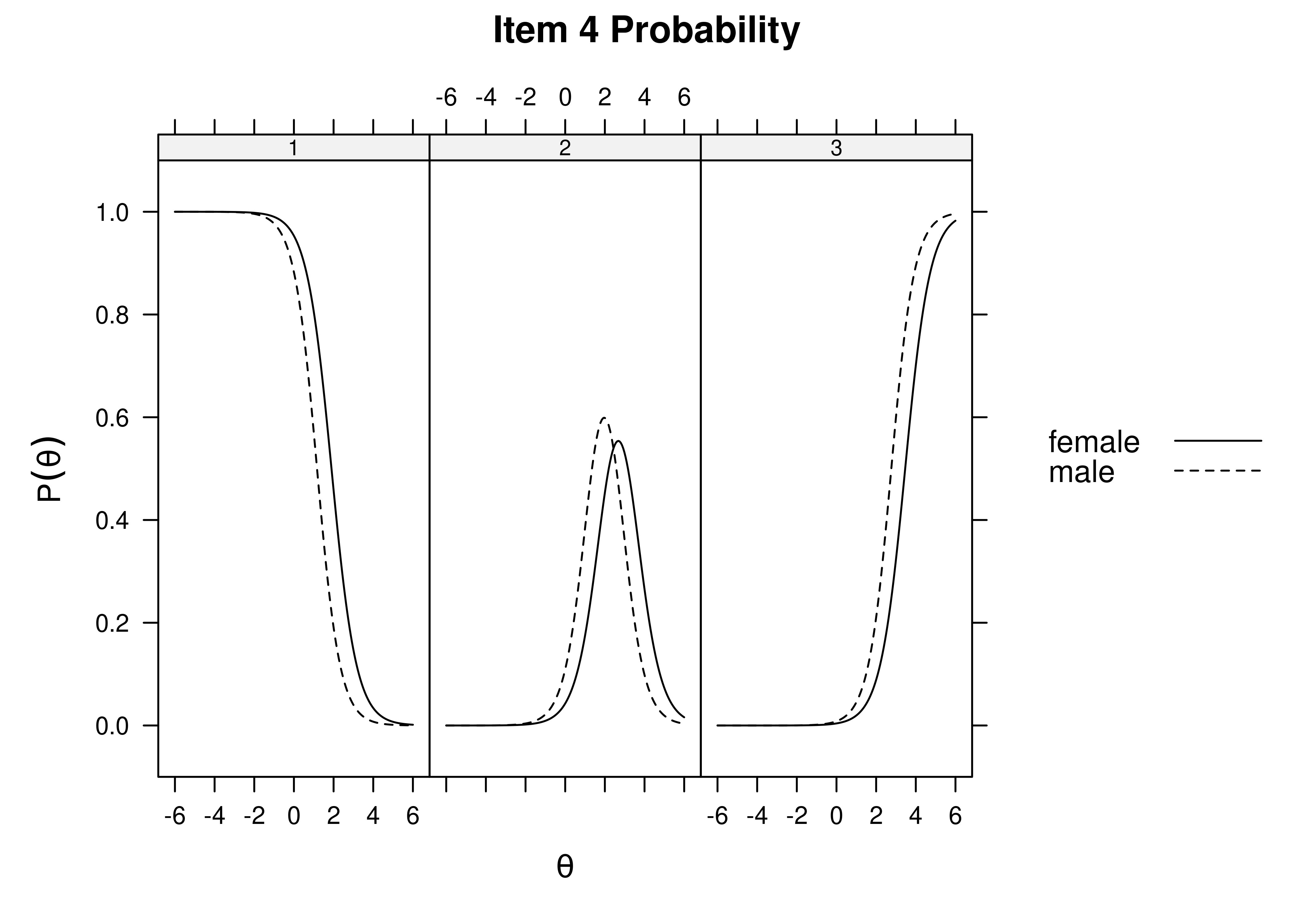
Figure 16.35: Item Response Category Characteristic Curves by Sex: Item 4.
Code
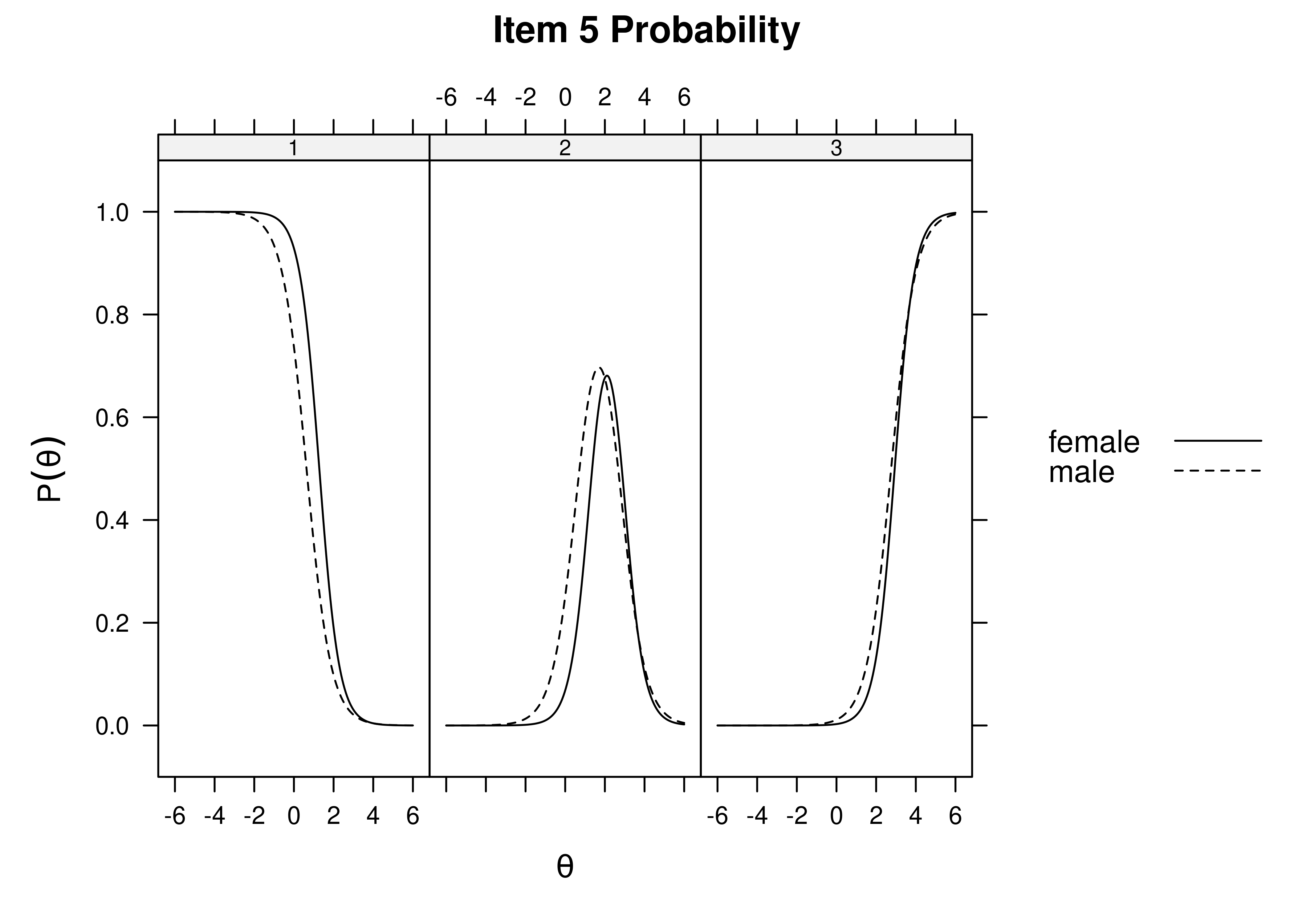
Figure 16.36: Item Response Category Characteristic Curves by Sex: Item 5.
Code
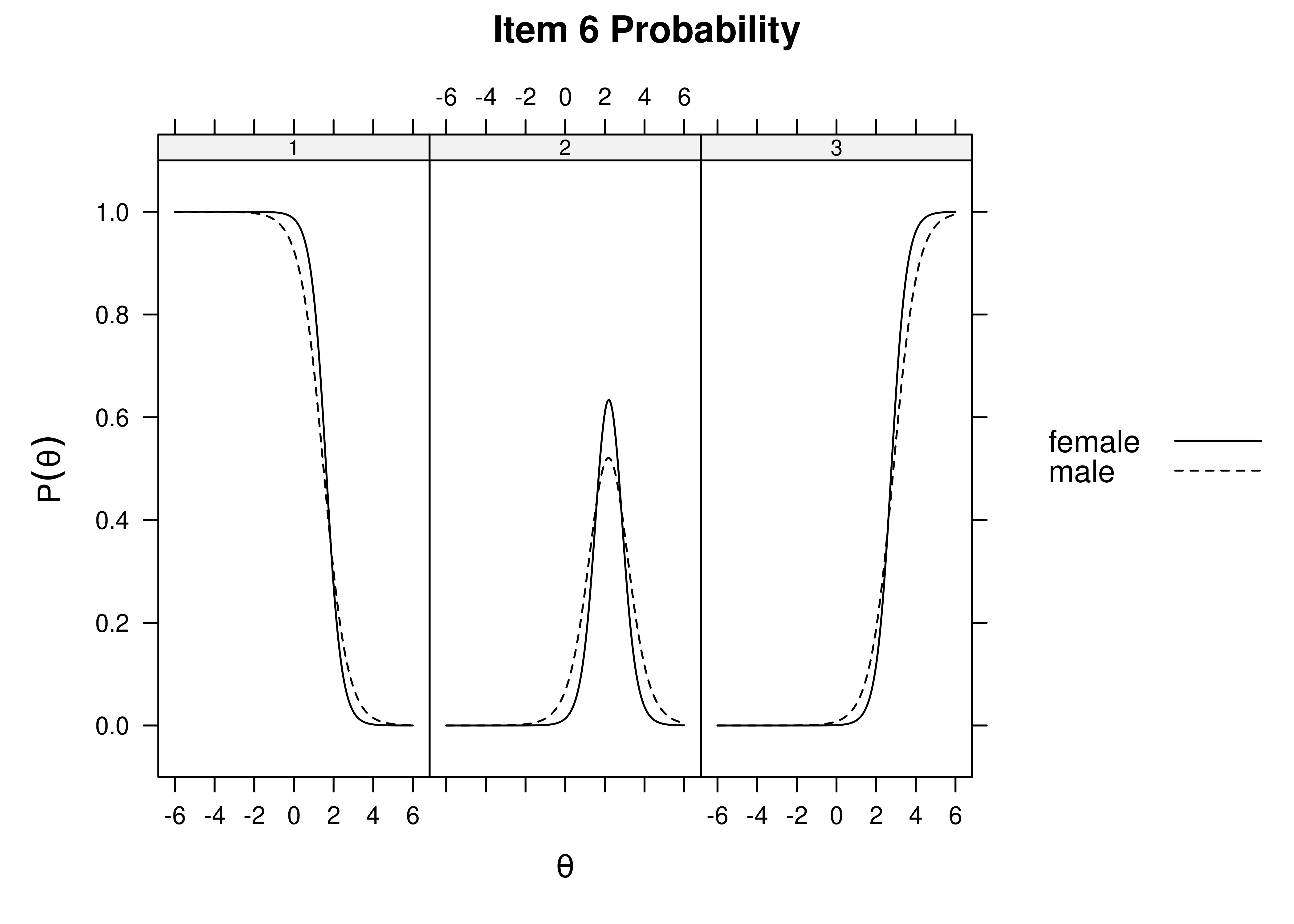
Figure 16.37: Item Response Category Characteristic Curves by Sex: Item 6.
Code
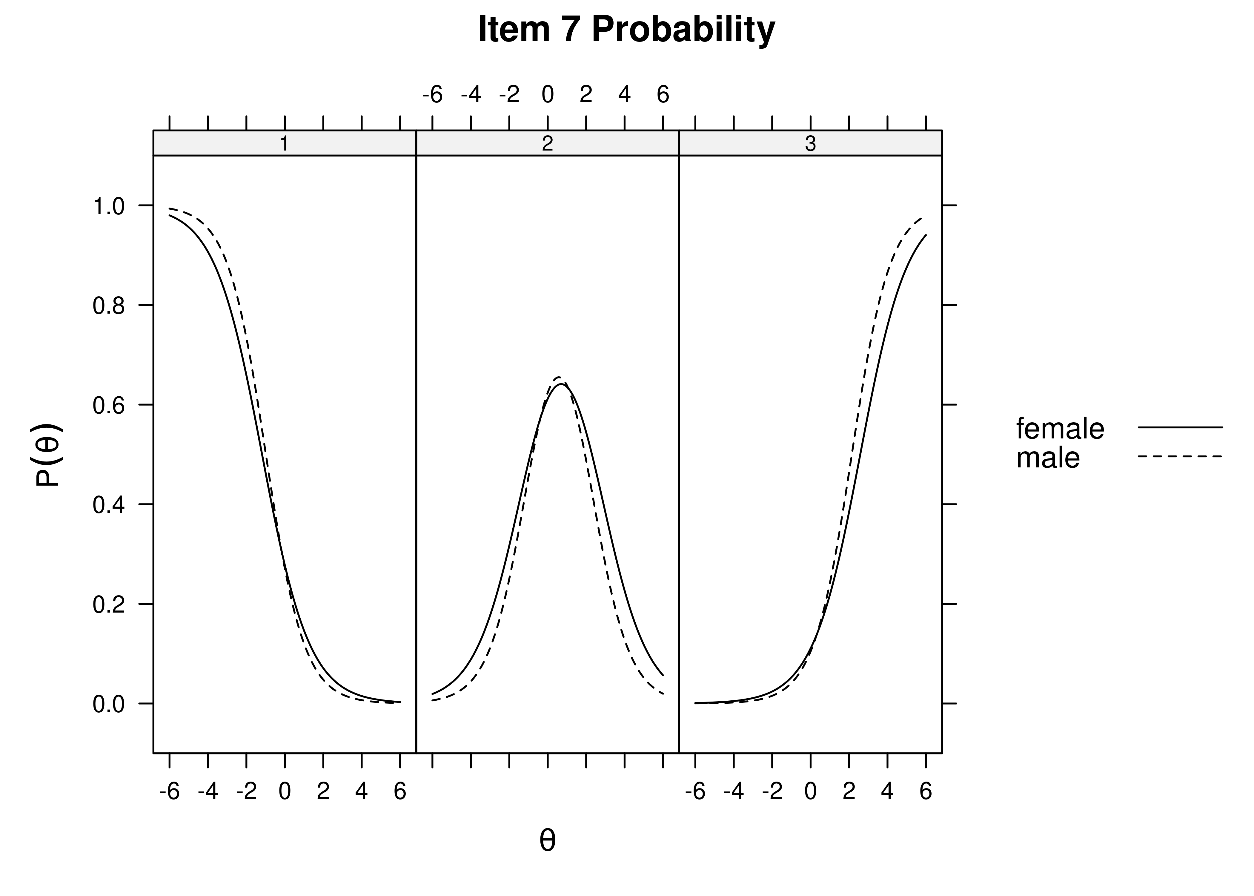
Figure 16.38: Item Response Category Characteristic Curves by Sex: Item 7.
Plots of item information functions by sex are in Figures 16.39–16.45 below. Items 1, 5, and 6 showed greater information for females than for males. Items 2, 4, and 7 showed greater information for females than for males.
Code
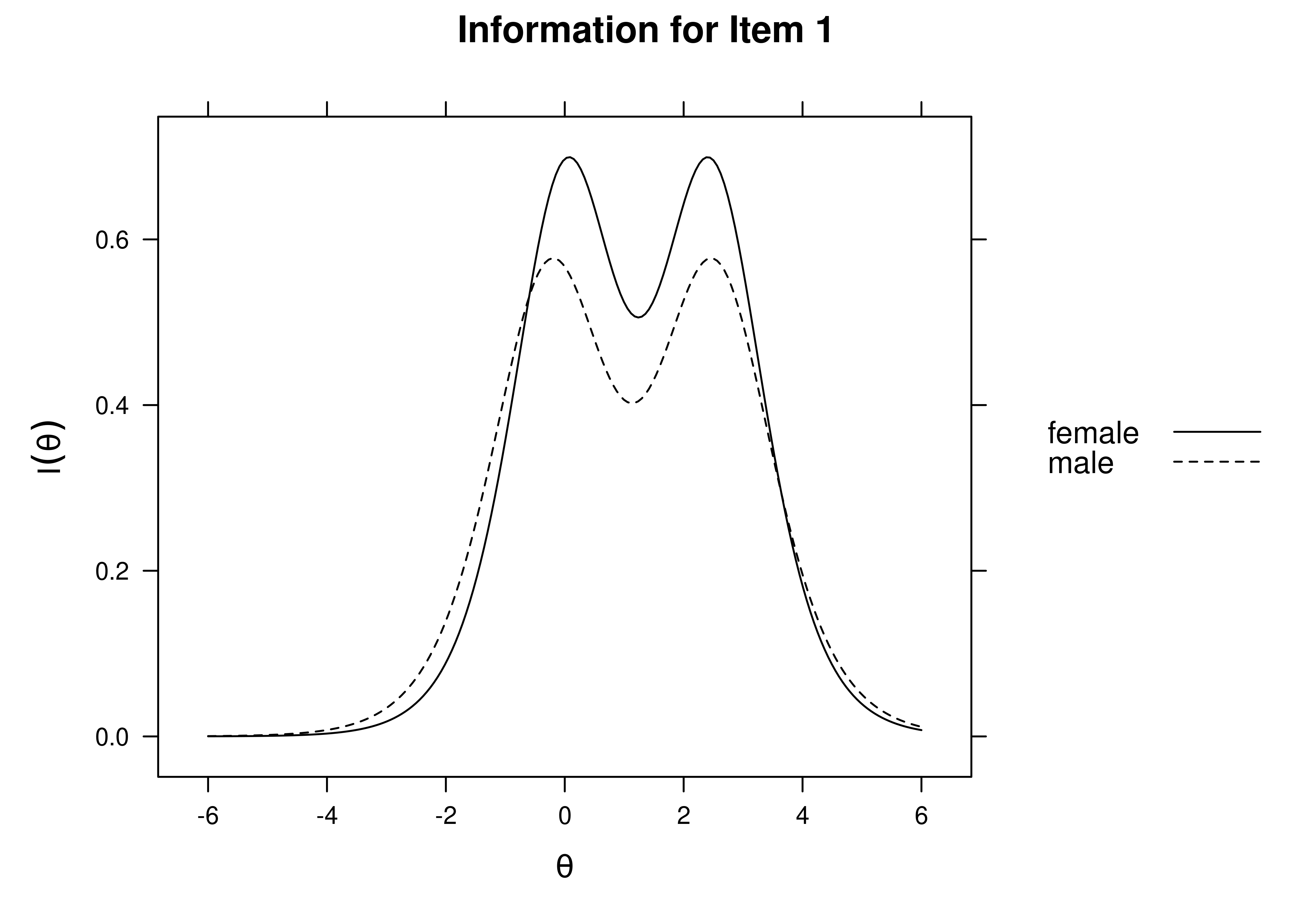
Figure 16.39: Item Information Curves by Sex: Item 1.
Code
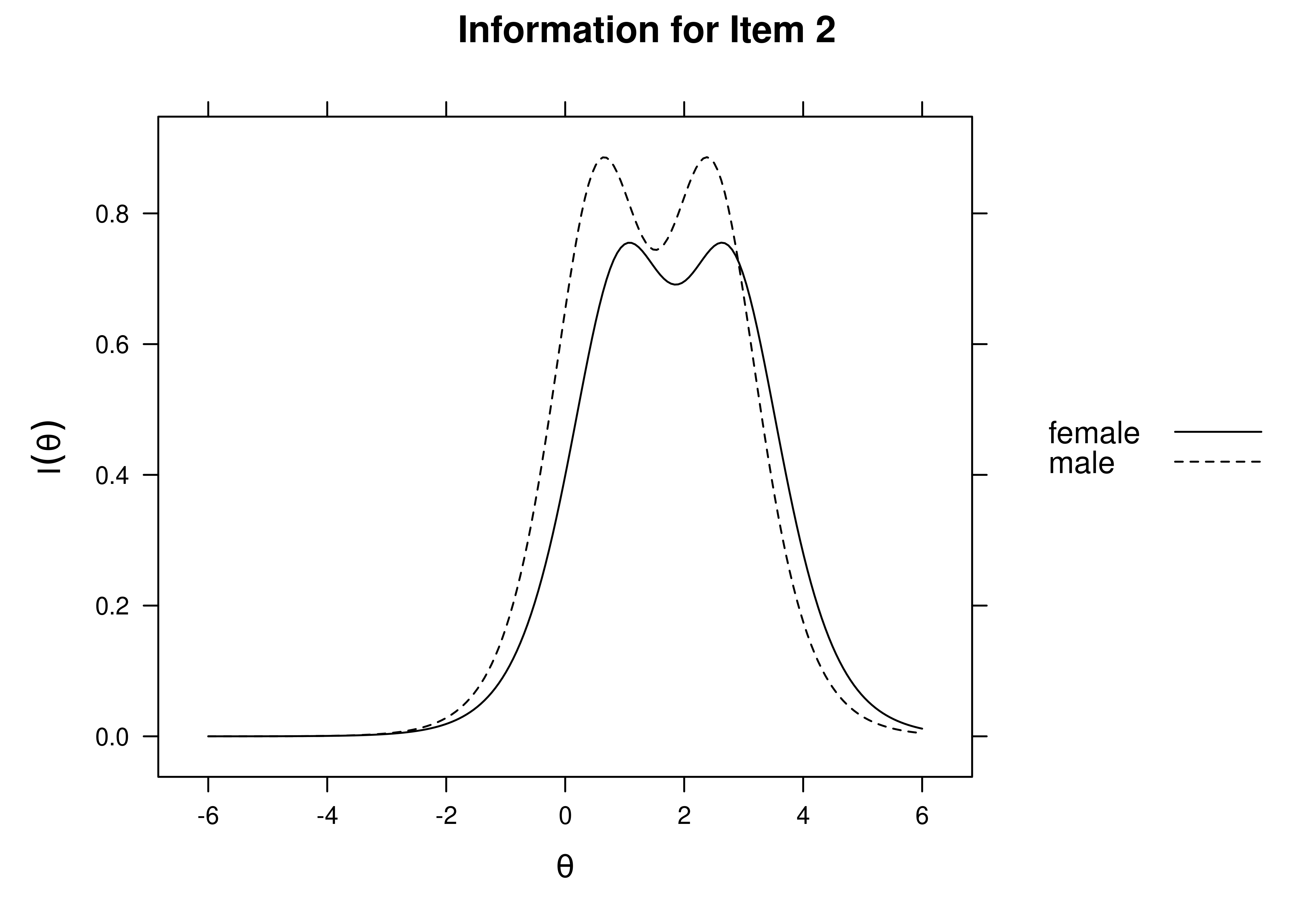
Figure 16.40: Item Information Curves by Sex: Item 2.
Code
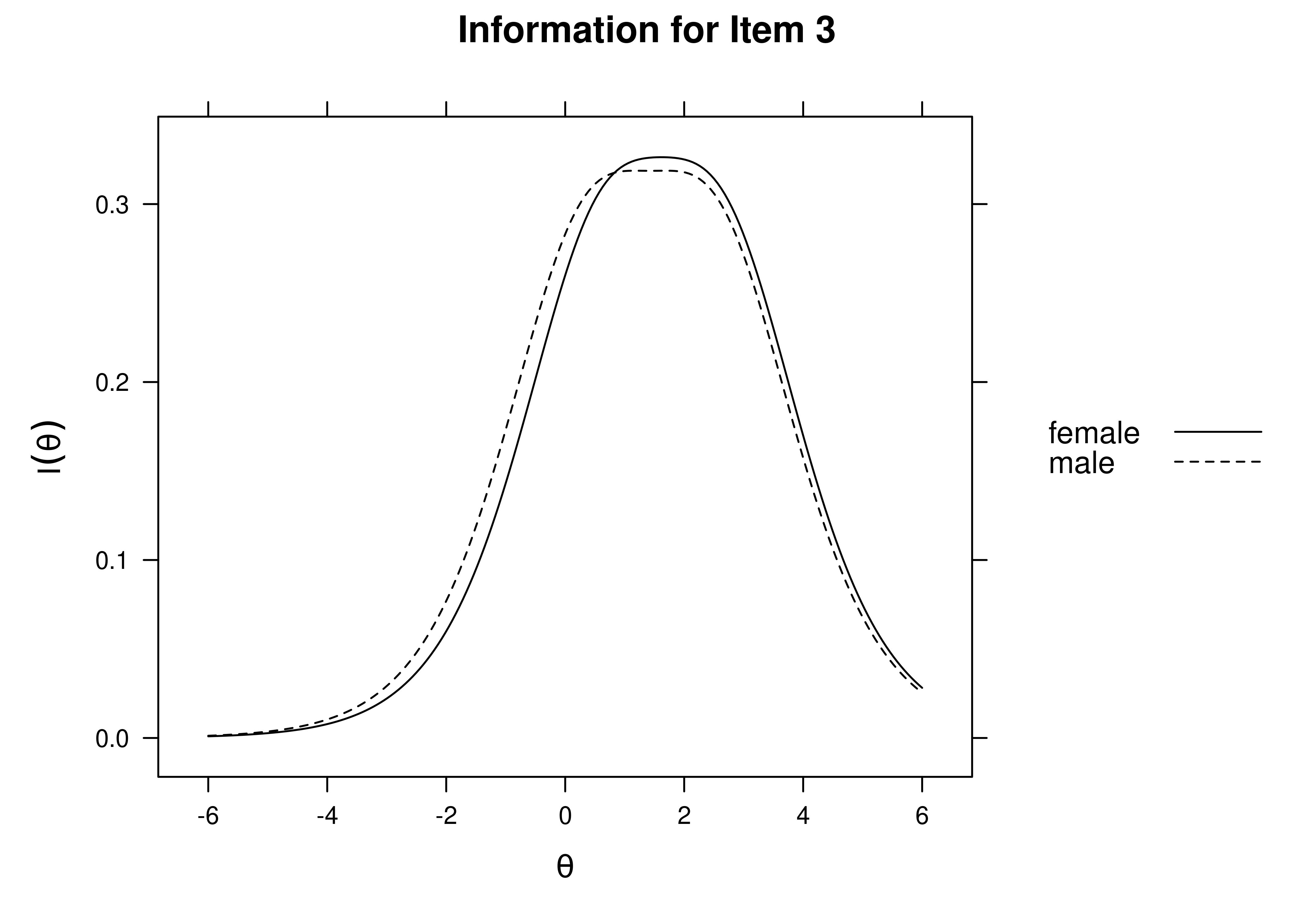
Figure 16.41: Item Information Curves by Sex: Item 3.
Code
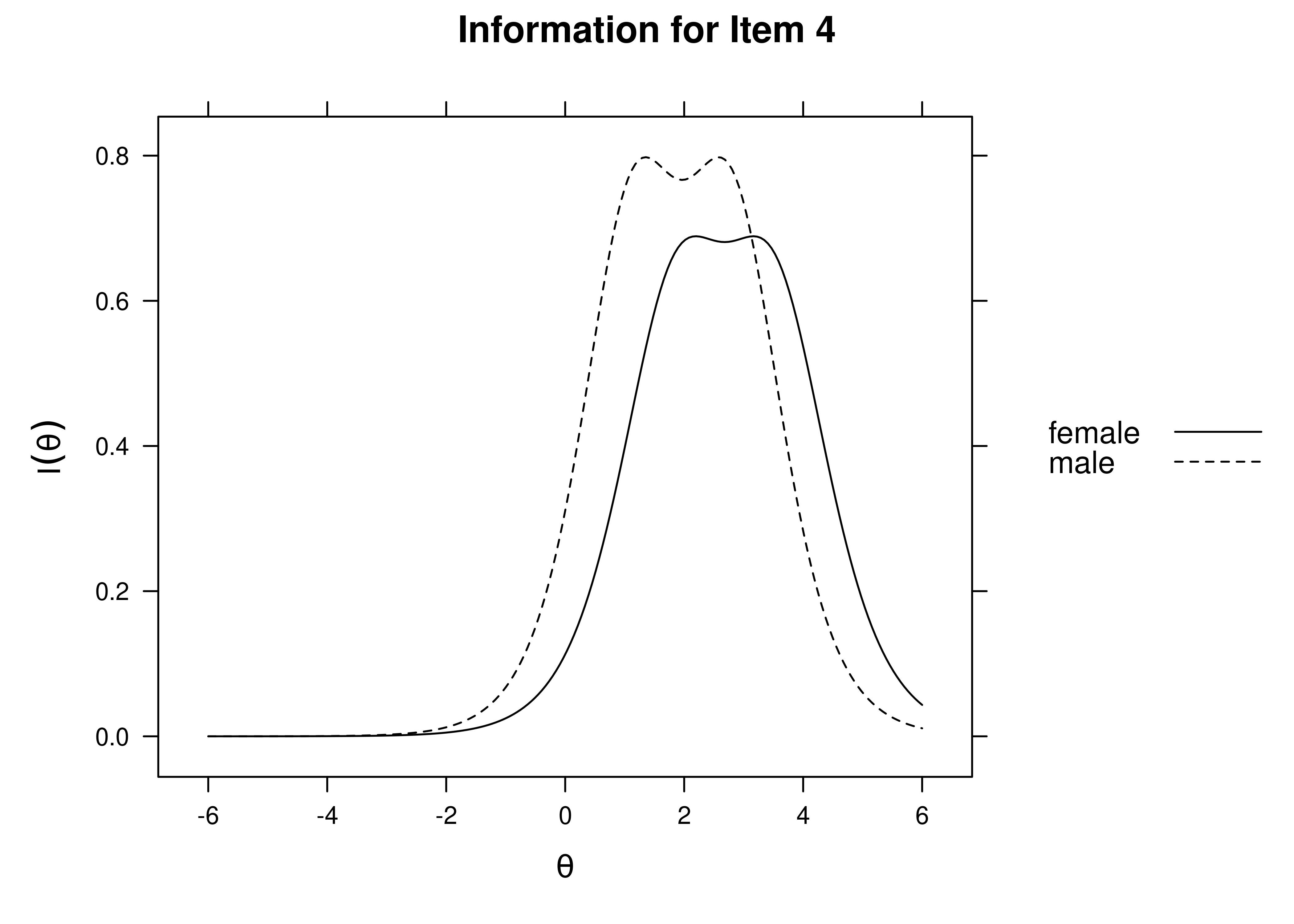
Figure 16.42: Item Information Curves by Sex: Item 4.
Code
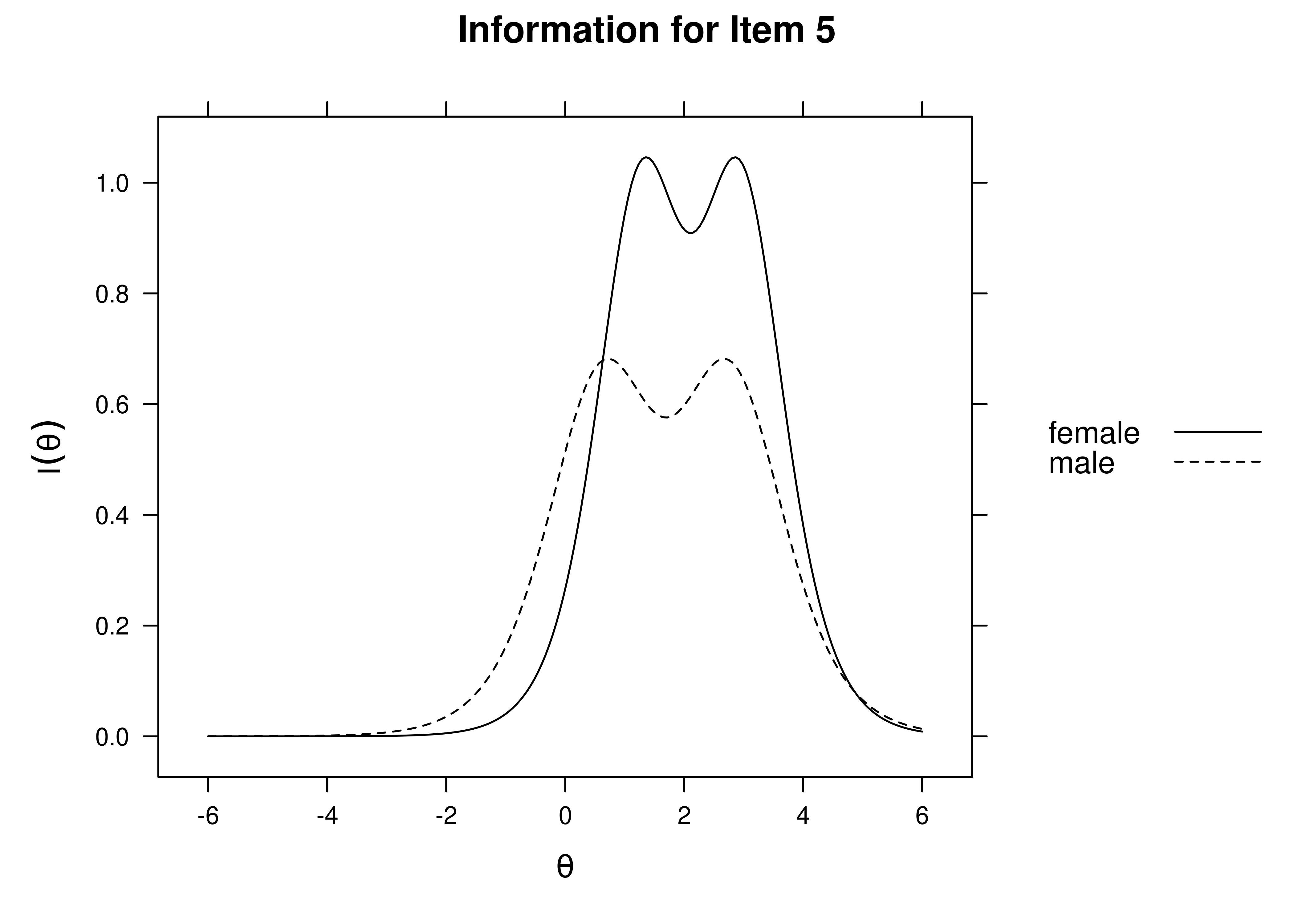
Figure 16.43: Item Information Curves by Sex: Item 5.
Code
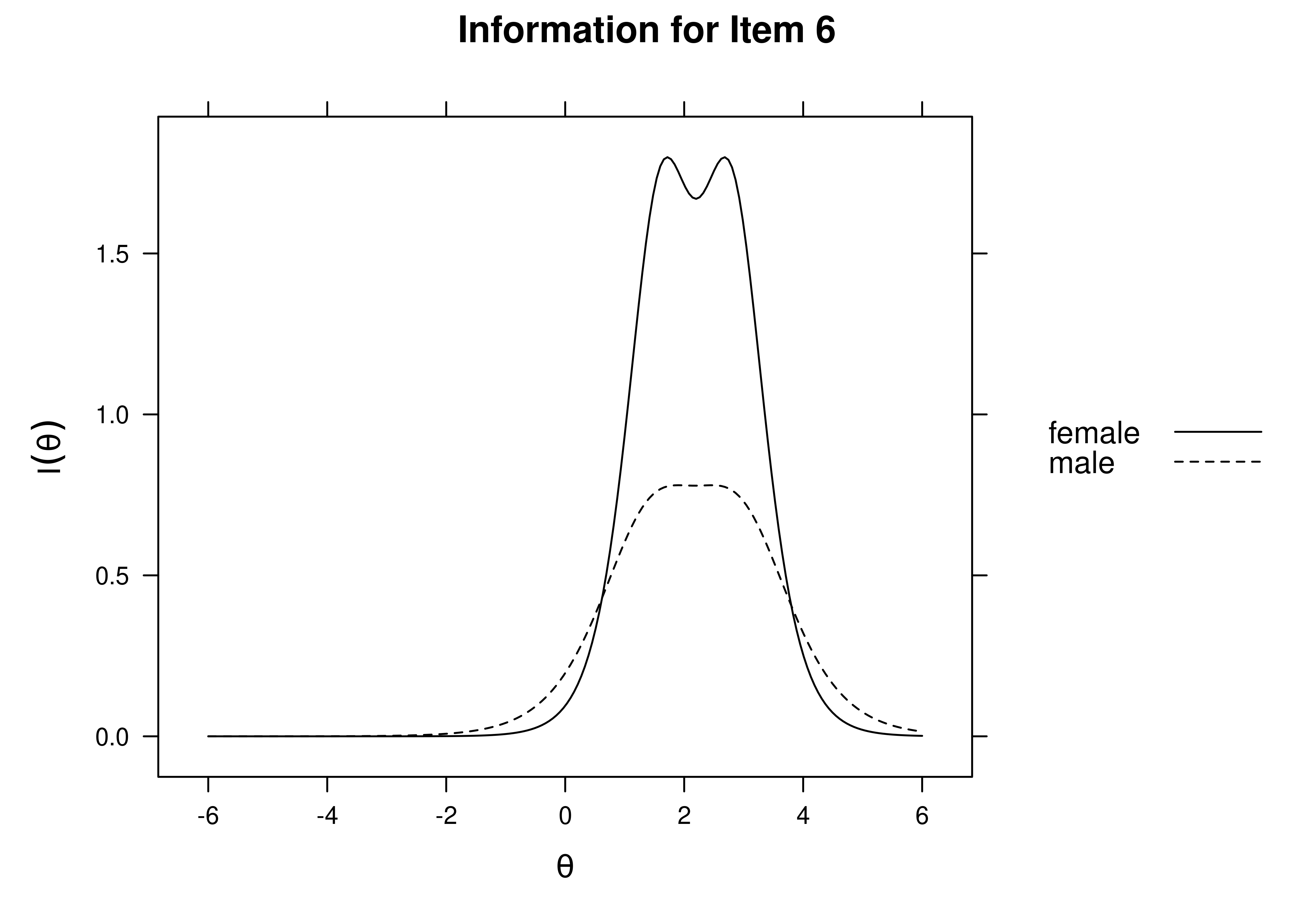
Figure 16.44: Item Information Curves by Sex: Item 6.
Code
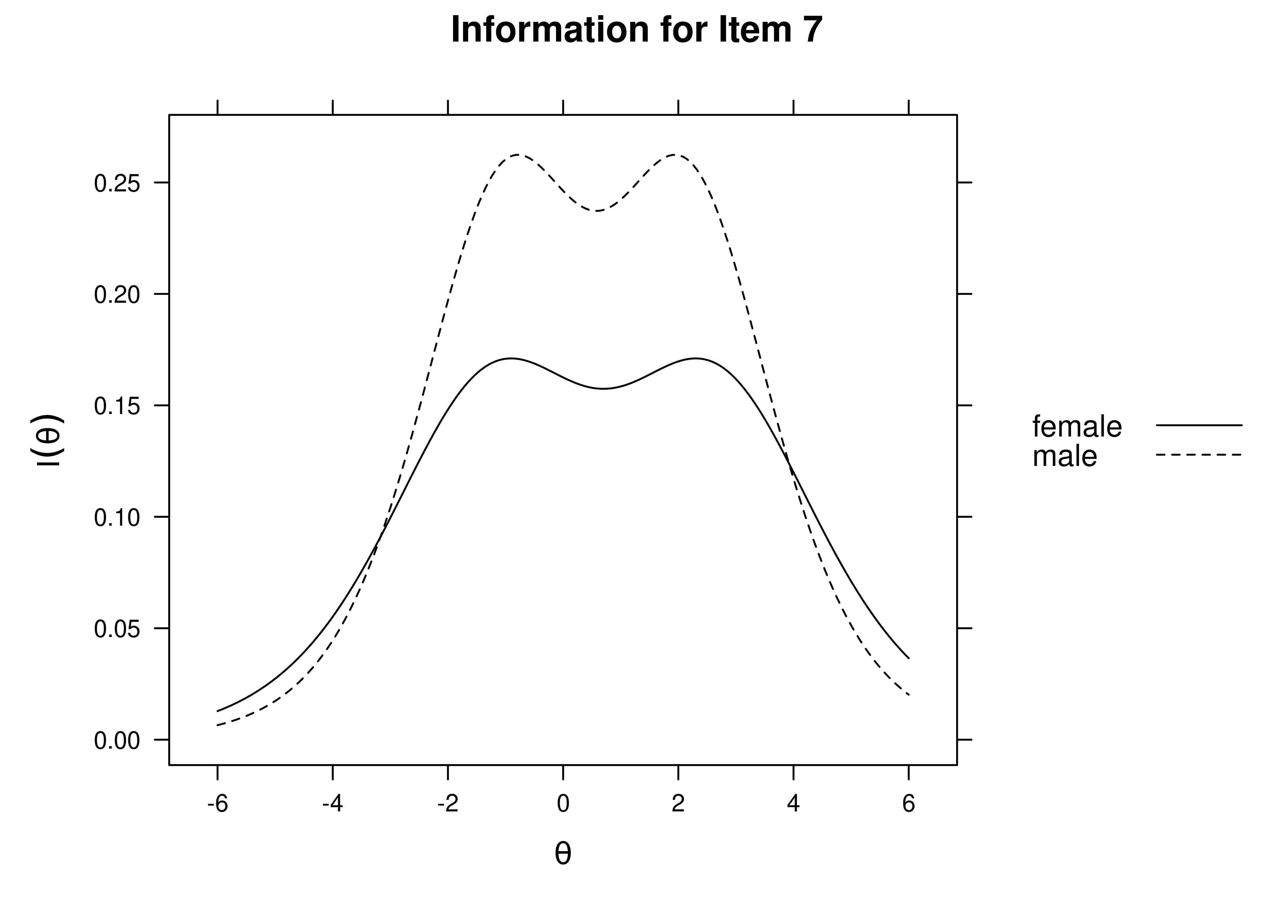
Figure 16.45: Item Information Curves by Sex: Item 7.
Plots of expected item scores by sex are are in Figures 16.46–16.52 below.
Code
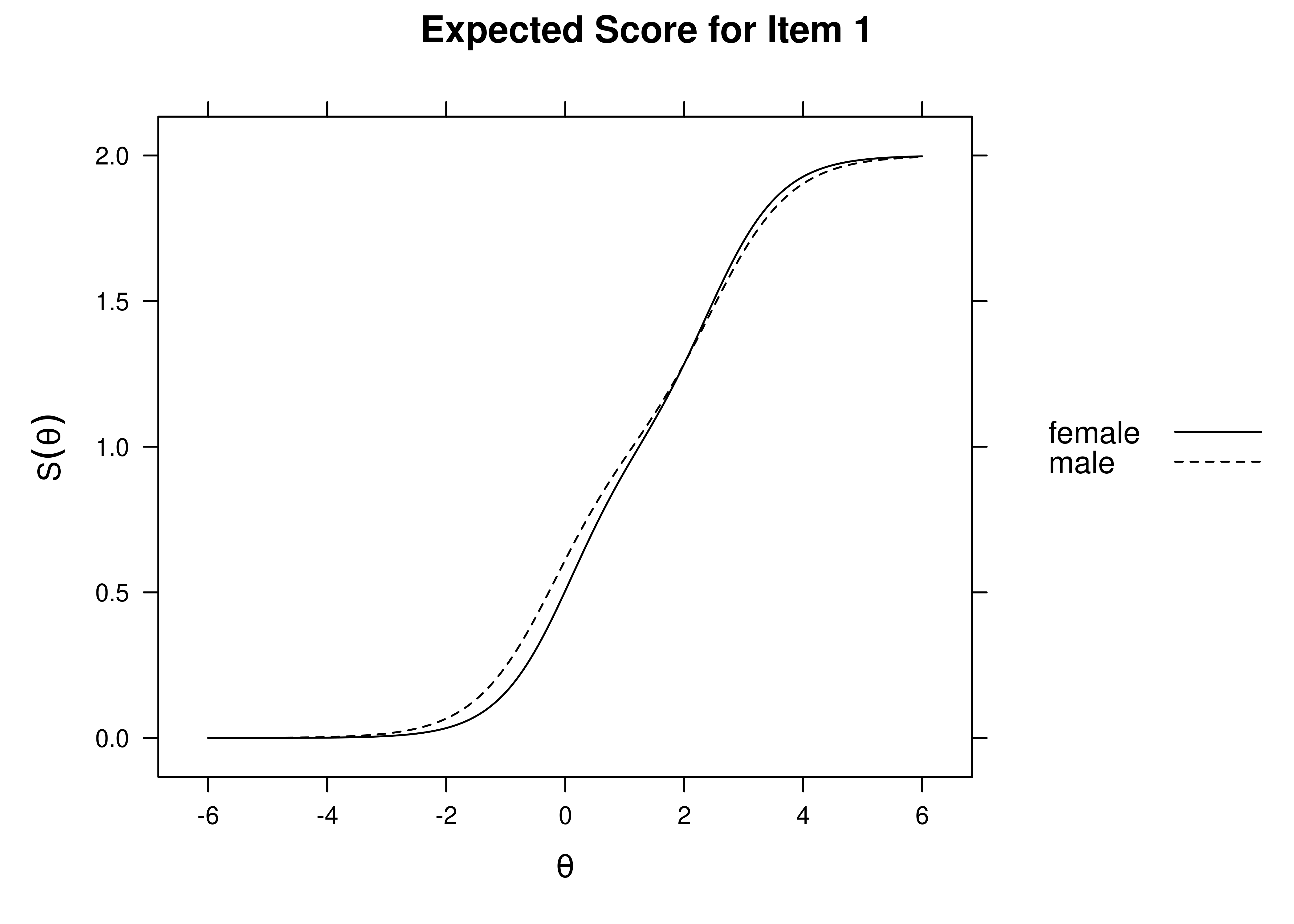
Figure 16.46: Expected Item Score by Sex: Item 1.
Code
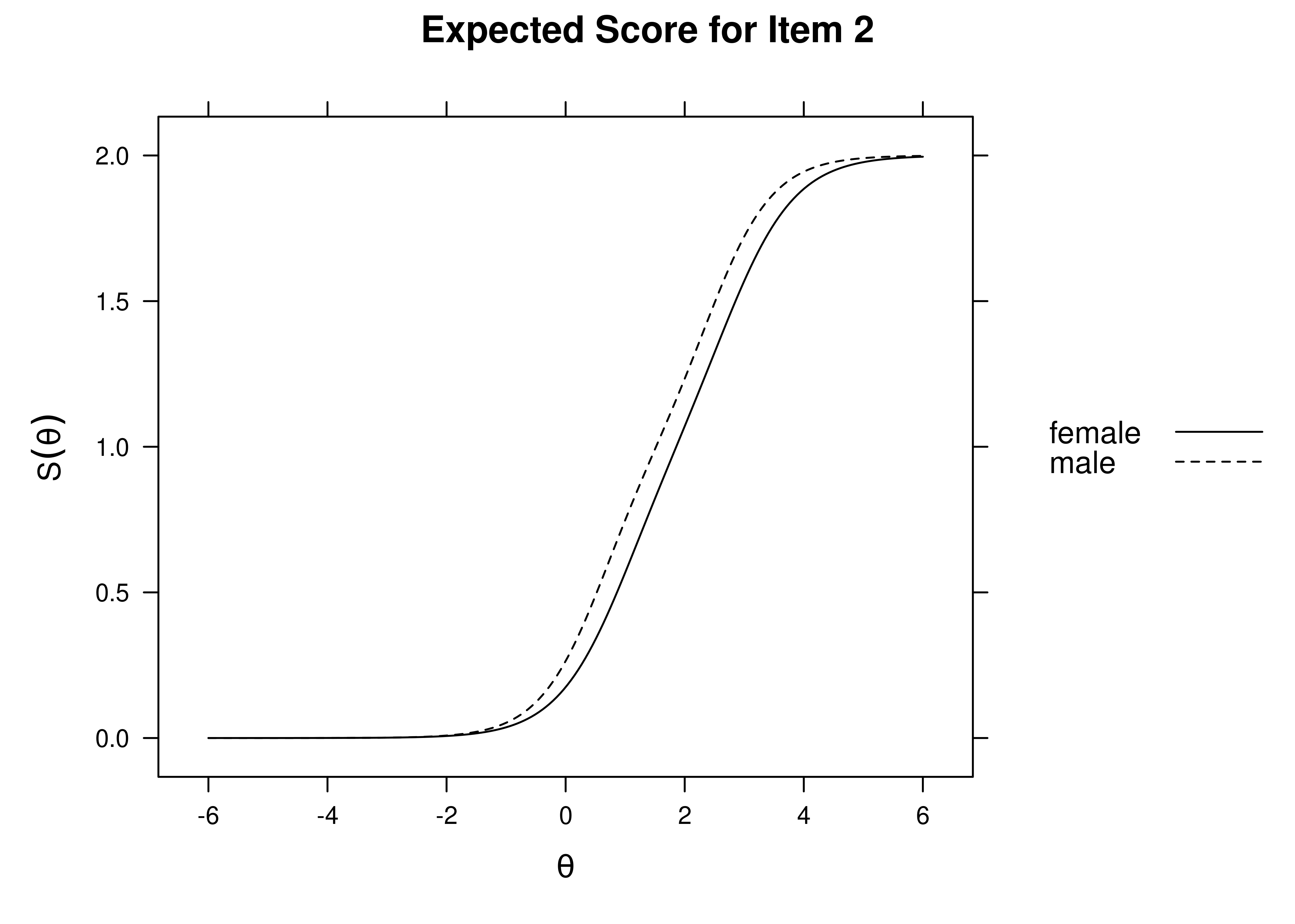
Figure 16.47: Expected Item Score by Sex: Item 2.
Code
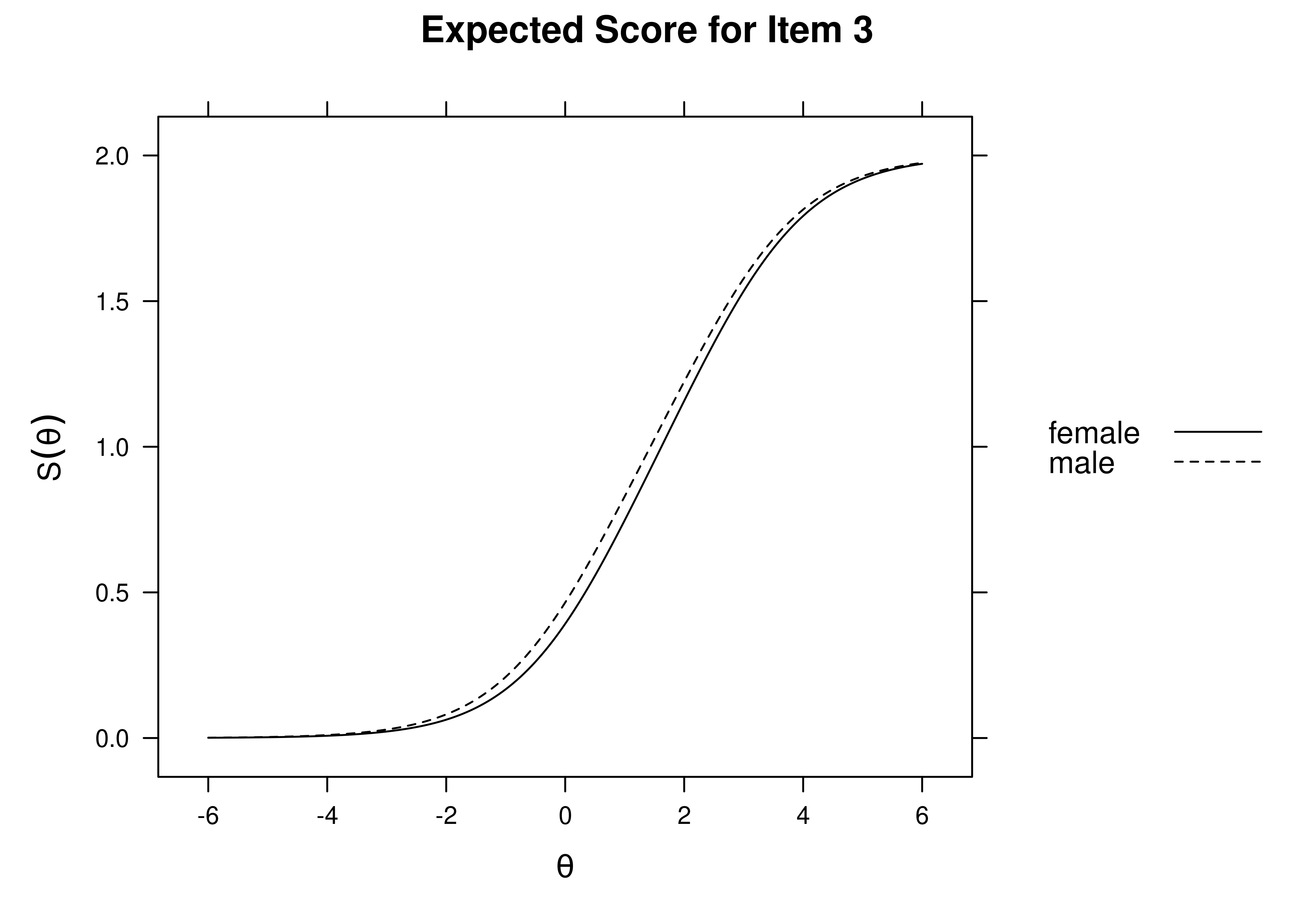
Figure 16.48: Expected Item Score by Sex: Item 3.
Code

Figure 16.49: Expected Item Score by Sex: Item 4.
Code
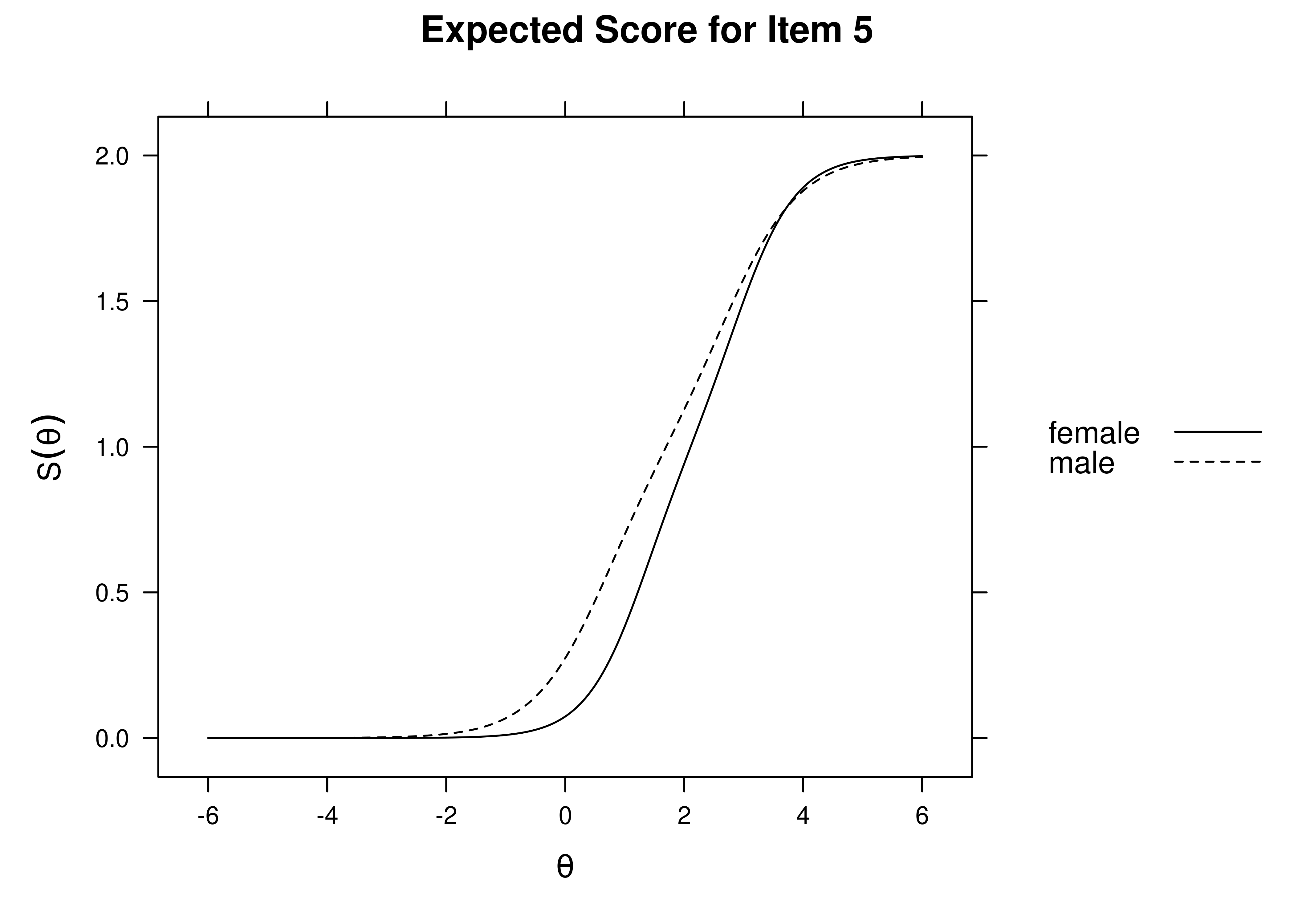
Figure 16.50: Expected Item Score by Sex: Item 5.
Code

Figure 16.51: Expected Item Score by Sex: Item 6.
Code

Figure 16.52: Expected Item Score by Sex: Item 7.
16.9.9 Addressing DIF
Based on the analyses above, item 5 shows the largest magnitude of DIF. Specifically, item 5 has a stronger discrimination parameter for women than men. So, we should handle item 5 first. If we deem the DIF for item 5 to be non-negligible, we have three primary options: (1) drop item 5 for both men and women, (2) drop item 5 for men but keep it for women, or (3) freely estimate the parameters (discrimination and difficulty) for item 5 across groups.
16.9.9.1 Drop item for both groups
The first option is to drop item 5 for both men and women groups. You might do this if you want to use a measure that has only those items that function equivalently across groups. However, this can lead to lower reliability and weaker ability to detect individual differences.
Code
constrainedModelDropItem5 <- multipleGroup(
  data = cnlsy[,c(
    "bpi_antisocialT1_1","bpi_antisocialT1_2","bpi_antisocialT1_3",
    "bpi_antisocialT1_4","bpi_antisocialT1_6","bpi_antisocialT1_7")],
  model = 1,
  group = cnlsy$sex,
  invariance = c(c(
    "bpi_antisocialT1_1","bpi_antisocialT1_2","bpi_antisocialT1_3",
    "bpi_antisocialT1_4","bpi_antisocialT1_6","bpi_antisocialT1_7"),
    "free_means", "free_var"),
  SE = TRUE)

coef(constrainedModelDropItem5, simplify = TRUE)
16.9.9.2 Drop item for one group but not another group
A second option is to drop item 5 for men but to keep it for women. You might do this if the item is invalid for men, but still valid for women. The coefficients show an item parameter for item 5 for men, but it was constrained to be equal to the parameter for women, and data were removed from the estimation of item 5 for men.
Code
dropItem5ForMen <- cnlsy
dropItem5ForMen[which(
  dropItem5ForMen$sex == "male"),
  "bpi_antisocialT1_5"] <- NA

constrainedModelDropItem5ForMen <- multipleGroup(
  data = dropItem5ForMen[,c(
    "bpi_antisocialT1_1","bpi_antisocialT1_2","bpi_antisocialT1_3",
    "bpi_antisocialT1_4","bpi_antisocialT1_5","bpi_antisocialT1_6",
    "bpi_antisocialT1_7")],
  model = 1,
  group = dropItem5ForMen$sex,
  invariance = c(c(
    "bpi_antisocialT1_1","bpi_antisocialT1_2","bpi_antisocialT1_3",
    "bpi_antisocialT1_4","bpi_antisocialT1_5","bpi_antisocialT1_6",
    "bpi_antisocialT1_7"),
    "free_means", "free_var"),
  SE = TRUE)

coef(constrainedModelDropItem5ForMen, simplify = TRUE)
16.9.9.3 Freely estimate item to have different parameters across groups
Alternatively, we can resolve DIF by allowing the item to have different parameters (discrimination and difficulty) across both groups. You might do this if the item is valid for both men and women, and it has importantly different item parameters nonetheless.
Code
constrainedModelResolveItem5 <- multipleGroup(
  data = cnlsy[,c(
    "bpi_antisocialT1_1","bpi_antisocialT1_2","bpi_antisocialT1_3",
    "bpi_antisocialT1_4","bpi_antisocialT1_5","bpi_antisocialT1_6",
    "bpi_antisocialT1_7")],
  model = 1,
  group = cnlsy$sex,
  invariance = c(c(
    "bpi_antisocialT1_1","bpi_antisocialT1_2","bpi_antisocialT1_3",
    "bpi_antisocialT1_4","bpi_antisocialT1_6","bpi_antisocialT1_7"),
    "free_means", "free_var"),
  SE = TRUE)

coef(constrainedModelResolveItem5, simplify = TRUE)
16.9.9.4 Compare model fit
We can compare the model fit against the fully constrained model. In this case, all three of these approaches for handling DIF resulted in improvement in model fit based on AIC and, for the two nested models, the chi-square difference test.
16.9.9.5 Next steps
Whichever of these approaches we select, we would then identify and handle the remaining non-negligent DIF sequentially by magnitude. For instance, if we chose to resolve DIF in item 5 by allowing the item to have different parameters across both groups, we would then iteratively drop constraints to see which items continue to show non-negligible DIF.
Code
| groups | converged | AIC | SABIC | HQ | BIC | X2 | df | p | |
|---|---|---|---|---|---|---|---|---|---|
| bpi_antisocialT1_1 | female,male | TRUE | -5.5042001 | 3.7824138 | 1.1738421 | 13.3150439 | 11.5042001 | 3 | 0.0092897 |
| bpi_antisocialT1_2 | female,male | TRUE | 3.8539227 | 13.1405366 | 10.5319649 | 22.6731667 | 2.1460773 | 3 | 0.5426474 |
| bpi_antisocialT1_3 | female,male | TRUE | 1.4534865 | 10.7401004 | 8.1315287 | 20.2727305 | 4.5465135 | 3 | 0.2081787 |
| bpi_antisocialT1_4 | female,male | TRUE | -26.4683563 | -17.1817424 | -19.7903141 | -7.6491123 | 32.4683563 | 3 | 0.0000004 |
| bpi_antisocialT1_5 | female,male | TRUE | 0.0000966 | 0.0000966 | 0.0000966 | 0.0000966 | -0.0000966 | 0 | NaN |
| bpi_antisocialT1_6 | female,male | TRUE | -9.9043878 | -0.6177739 | -3.2263456 | 8.9148562 | 15.9043878 | 3 | 0.0011863 |
| bpi_antisocialT1_7 | female,male | TRUE | -16.5941405 | -7.3075266 | -9.9160983 | 2.2251035 | 22.5941405 | 3 | 0.0000491 |
Estimates of DIF after resolving item 5 are in Table 16.1. Of the remaining DIF, item 4 appears to have the largest DIF. If we deem item 4 to show non-negligible DIF, we would address it using one of the three approaches above and then see which items continue to show the largest DIF, address it if necessary, then identify the remaining DIF, etc.
16.10 Measurement/Factorial Invariance
Before making comparisons across groups in terms of associations between constructs or their level on the construct, it is important to establish measurement invariance (also called factorial invariance) across the groups (Millsap, 2011). Tests of measurement invariance are equivalent to tests of differential item functioning. Measurement invariance can help provide greater confidence that the measure functions equivalently across groups, that is, the items have the same strength of association with the latent factor, and the latent factor is on the same metric (i.e., the items have the same level when accounting for the latent factor). For instance, If you observe differences between groups in level of depression without establishing measurement invariance across the groups, you do not know whether the differences observed reflect true group-related differences in depression or differences in the functioning of the measure across the groups.
Measurement invariance can be tested using many methods, including confirmatory factor analysis and IRT. CFA approaches to testing measurement invariance include multi-group CFA (MGCFA), multiple-indicator, multiple-causes (MIMIC) models, moderated nonlinear factor analysis (MNLFA), score-based tests (T. Wang et al., 2014), and the alignment method (Lai, 2021). The IRT approach to testing measurement (non-)invariance is to examine whether items show differential item functioning.
The tests of measurement invariance in confirmatory factor analysis (CFA) models were fit in the lavaan package (Rosseel et al., 2022).
The examples were adapted from lavaan documentation: https://lavaan.ugent.be/tutorial/groups.html (archived at https://perma.cc/2FBK-RSAH).
Procedures for testing measurement invariance are outlined in Putnick & Bornstein (2016).
In addition to nested chi-square difference tests (\(\chi^2_{\text{diff}}\)), I also demonstrate permutation procedures for testing measurement invariance, as described by Jorgensen et al. (2018).
Also, you are encouraged to read about MIMIC models (Cheng et al., 2016; W.-C. Wang et al., 2009), score-based tests (T. Wang et al., 2014), and MNLFA that allows for testing measurement invariance across continuous moderators (Bauer et al., 2020; Curran et al., 2014; N. C. Gottfredson et al., 2019).
MNLFA is implemented in the mnlfa package (Robitzsch, 2019).
You can also generate syntax for conducting MNLFA in Mplus software (Muthén & Muthén, 2019) using the aMNLFA package (V. Cole et al., 2018).
The alignment method allows many groups to be compared (Han et al., 2019).
Model fit of nested models can be compared with a chi-square difference test, as a way of testing measurement invariance. In this approach to testing measurement invariance, first model fit is evaluated in a configural invariance model, in which the same number of factors is specified in each group, and which indicators load on which factors are the same in each group. Then, successive constraints are made across groups, including constraining factor loadings, intercepts, and residuals across groups. The metric (“weak factorial”) invariance model is similar to the configural invariance model, but it constrains the factor loadings to be the same across groups. The scalar (“strong factorial”) invariance model keeps the constraints of the metric invariance model, but it also constrains the intercepts to be the same across groups. The residual (“strict factorial”) invariance model keeps the constraints of the scalar invariance model, but it also constrains the residuals to be the same across groups. The fit of each constrained model is compared to the previous model without such constraints. That is, the fit of the metric invariance model is compared to the fit of the configural invariance model, the fit of the scalar invariance model is compared to the fit of the metric invariance model, and the fit of the residual invariance model is compared to the fit of the scalar invariance model.
The chi-square difference test is sensitive to sample size, and trivial differences in fit can be detected with large samples (Cheung & Rensvold, 2002). As a result, researchers also recommend examining change in additional criteria, including CFI, RMSEA, and SRMR (F. F. Chen, 2007). Cheung & Rensvold (2002) recommend a cutoff of \(\Delta \text{CFI} \geq -.01\) for identifying measurement non-invariance. F. F. Chen (2007) recommends the following cutoffs for identifying measurement non-invariance:
- with a small sample size (total \(N \leq 300\)):
- testing invariance of factor loadings:
- \(\Delta \text{CFI} \geq -.005\)
- supplemented by \(\Delta \text{RMSEA} \geq .010\) or \(\Delta \text{SRMR} \geq .025\)
- testing invariance of intercepts or residuals:
- \(\Delta \text{CFI} \geq -.005\)
- supplemented by \(\Delta \text{RMSEA} \geq .010\) or \(\Delta \text{SRMR} \geq .005\)
- testing invariance of factor loadings:
- with an adequate sample size (total \(N > 300\)):
- testing invariance of factor loadings:
- \(\Delta \text{CFI} \geq -.010\)
- supplemented by \(\Delta \text{RMSEA} \geq .015\) or \(\Delta \text{SRMR} \geq .030\)
- testing invariance of intercepts or residuals:
- \(\Delta \text{CFI} \geq -.005\)
- supplemented by \(\Delta \text{RMSEA} \geq .015\) or \(\Delta \text{SRMR} \geq .010\)
- testing invariance of factor loadings:
Little et al. (2007) suggested that researchers establish at least partial invariance of factor loadings (metric invariance) to compare covariances across groups, and at least partial invariance of intercepts (scalar invariance) to compare mean levels across groups. Partial invariance refers to invariance with some but not all indicators. So, to examine associations with other variables, invariance of at least some factor loadings would be preferable. To examine differences in level or growth, invariance of at least some factor loadings and intercepts would be preferable. Residual invariance is considered overly restrictive, and it is not generally expected that one establish residual invariance (Little, 2013).
Although measurement invariance is important to test, it is also worth noting that tests of measurement invariance and DIF rest on various fundamentally untestable assumptions related to scale setting (Raykov et al., 2020). For instance, to give the latent factor units, oftentimes researchers set one item’s factor loading to be equal across time (i.e., the marker variable). Results of factorial invariance tests can depend highly on which item is used as the anchor item for setting the scale of the latent factor (Belzak & Bauer, 2020). And subsequent tests of measurement invariance then rest on the fundamentally untestable assumption that changes in the level of the latent factor precipitates the same amount of change in the item across groups. If this scaling is not proper, however, it could lead to improper conclusions. Researchers are, therefore, not conclusively able to establish measurement invariance.
Several possible approaches may help address this. First, it can be helpful to place greater focus on degree of measurement invariance and confidence (rather than presence versus absence of measurement invariance). To the extent that non-invariance is trivial in effect size, it provides the researcher with greater confidence that they can use the measure to assess a construct in a comparable way over time.
Second, there may be important robustness checks. I describe each in greater detail below. One important sensitivity analysis could be to see if measurement invariance holds when using different marker variables. This would provide greater evidence that their apparent measurement invariance was not specific to one marker variable (i.e., one particular set of assumptions). A second robustness check would be to use effects coding, in which the average of items’ factor loadings is equal to 1, so the metric of the latent variable is on the metric of all of the items rather than just one item (Little et al., 2006). A third robustness check would be to use regularization, which is an alternative method to select the anchor items and to identify differential item functioning based on a machine learning technique that applies penalization to remove parameters that have little impact on model fit (Bauer et al., 2020; Belzak & Bauer, 2020).
Another issue with measurement invariance is that the null hypothesis that adding constraints across groups will not worsen fit is likely always false, because there are often at least slight differences across groups in factor loadings, intercepts, or residuals that reflect sampling variability. However, we are not interested in trivial differences across groups that reflect sampling variability. Instead, we are interested in the extent to which there are substantive, meaningful differences across the groups of large enough magnitude to be practically meaningful. Thus, it can also be helpful to consider whether the measures show approximate measurement invariance (Van De Schoot et al., 2015). For details on how to test approximate measurement invariance, see Van De Schoot et al. (2013).
When detecting measurement non-invariance in a given parameter (e.g., factor loadings, intercepts, or residuals), one can identify the specific items that show measurement non-invariance in one of two primary ways: (1) starting with a model that allows the given parameter to differ across groups, a researcher can iteratively add constraints to identify the item(s) for which measurement invariance fails, or (2) starting with a model that constrains the given parameter to be the same across groups, a researcher can iteratively remove constraints to identify the item(s) for which measurement invariance becomes established (and by process of elimination, the items for which measurement invariance does not become established).
Approaches to addressing measurement non-invariance are described in Section 16.5.1. If we identify that an item shows non-negligible non-invariance, we have three primary options (described above): (1) drop the item for both groups, (2) drop the item for one group but keep it for the other group, or (3) freely estimate the parameters (factor loadings and/or intercepts) for the item across groups.
Using the traditional chi-square difference test, tests of measurement invariance compare the model fit to a model with perfect fit. As the sample size grows larger, smaller differences in model fit will be detected as significant, thus rejecting measurement invariance even if the model fits well. So, it can also be useful to compare the model fit to a null hypothesis that the fit is poor, instead of the null hypothesis that the model is a perfect fit. Chi-square equivalence tests use the poor model fit as the null hypothesis. Thus, a significant chi-square equivalence test suggests that the equality constraints are plausible, providing support for the alternative hypothesis that the model fit is acceptable (Counsell et al., 2020).
16.10.1 Effect Size of Measurement Non-Invariance
A number of studies describe how to test the effect size of measurement invariance (Gunn et al., 2020; e.g., Liu et al., 2017; Newsom, 2015; Nye et al., 2019) or differential item functioning (Gonzalez & Pelham, 2021; e.g., Meade, 2010). Indices of effect size of measurement noninvariance include \(d_{\text{MACS}}\) (Nye et al., 2019), \(w\) (Newsom, 2015), and \(\Delta \text{M}_\text{C}\) (Newsom, 2015).
\(w\) is interpreted such that .1, .3, and .5 indicate a small, medium, and large effect size, respectively. \(w\) is computed as in Equation (16.1) (Newsom, 2015):
\[\begin{equation} w = \sqrt{\frac{\Delta \chi^2}{N(\Delta df)}} \tag{16.1} \end{equation}\]
McDonald’s centrality index (\(\text{M}_\text{C}\)) is computed as in Equation (16.2) (Newsom, 2015):
\[\begin{equation} \text{M}_\text{C} = \exp\!\left[-\tfrac{1}{2}\,\left(\frac{\chi^{2} - \text{df}}{N - 1}\right)\right] \tag{16.2} \end{equation}\]
Then, \(\Delta \text{M}_\text{C}\) is computed as in Equation (16.3) (Newsom, 2015):
\[\begin{equation} \Delta \text{M}_\text{C} = \text{M}_{\text{C},\text{unconstrained}} - \text{M}_{\text{C},\text{constrained}} \tag{16.3} \end{equation}\]
16.10.2 Specify Models
16.10.2.1 Null Model
Fix residual variances and intercepts of manifest variables to be equal across groups.
Code
nullModel <- '
#Fix residual variances of manifest variables to be equal across groups
x1 ~~ c(psi1, psi1)*x1
x2 ~~ c(psi2, psi2)*x2
x3 ~~ c(psi3, psi3)*x3
x4 ~~ c(psi4, psi4)*x4
x5 ~~ c(psi5, psi5)*x5
x6 ~~ c(psi6, psi6)*x6
x7 ~~ c(psi7, psi7)*x7
x8 ~~ c(psi8, psi8)*x8
x9 ~~ c(psi9, psi9)*x9

#Fix intercepts of manifest variables to be equal across groups
x1 ~ c(tau1, tau1)*1
x2 ~ c(tau2, tau2)*1
x3 ~ c(tau3, tau3)*1
x4 ~ c(tau4, tau4)*1
x5 ~ c(tau5, tau5)*1
x6 ~ c(tau6, tau6)*1
x7 ~ c(tau7, tau7)*1
x8 ~ c(tau8, tau8)*1
x9 ~ c(tau9, tau9)*1
'16.10.2.3 Configural Invariance
Specify the same number of factors in each group, and which indicators load on which factors are the same in each group.
Code
cfaModel_configuralInvariance <- '
 #Factor loadings (free the factor loading of the first indicator)
 visual  =~ NA*x1 + x2 + x3
 textual =~ NA*x4 + x5 + x6
 speed   =~ NA*x7 + x8 + x9

 #Fix latent means to zero
 visual ~ 0
 textual ~ 0
 speed ~ 0

 #Fix latent variances to one
 visual ~~ 1*visual
 textual ~~ 1*textual
 speed ~~ 1*speed

 #Estimate covariances among latent variables
 visual ~~ textual
 visual ~~ speed
 textual ~~ speed

 #Estimate residual variances of manifest variables
 x1 ~~ x1
 x2 ~~ x2
 x3 ~~ x3
 x4 ~~ x4
 x5 ~~ x5
 x6 ~~ x6
 x7 ~~ x7
 x8 ~~ x8
 x9 ~~ x9

 #Free intercepts of manifest variables
 x1 ~ NA*1
 x2 ~ NA*1
 x3 ~ NA*1
 x4 ~ NA*1
 x5 ~ NA*1
 x6 ~ NA*1
 x7 ~ NA*1
 x8 ~ NA*1
 x9 ~ NA*1
'
16.10.2.4 Metric (“Weak Factorial”) Invariance
Specify invariance of factor loadings across groups.
Code
cfaModel_metricInvariance <- '
 #Fix factor loadings to be the same across groups
 visual  =~ c(lambdax1,lambdax1)*x1 + c(lambdax2,lambdax2)*x2 + c(lambdax3,lambdax3)*x3
 textual =~ c(lambdax4,lambdax4)*x4 + c(lambdax5,lambdax5)*x5 + c(lambdax6,lambdax6)*x6
 speed   =~ c(lambdax7,lambdax7)*x7 + c(lambdax8,lambdax8)*x8 + c(lambdax9,lambdax9)*x9

 #Fix latent means to zero
 visual ~ 0
 textual ~ 0
 speed ~ 0

 #Fix latent variances to one in group 1; free latent variances in group 2
 visual ~~ c(1, NA)*visual
 textual ~~ c(1, NA)*textual
 speed ~~ c(1, NA)*speed

 #Estimate covariances among latent variables
 visual ~~ textual
 visual ~~ speed
 textual ~~ speed

 #Estimate residual variances of manifest variables
 x1 ~~ x1
 x2 ~~ x2
 x3 ~~ x3
 x4 ~~ x4
 x5 ~~ x5
 x6 ~~ x6
 x7 ~~ x7
 x8 ~~ x8
 x9 ~~ x9

 #Free intercepts of manifest variables
 x1 ~ NA*1
 x2 ~ NA*1
 x3 ~ NA*1
 x4 ~ NA*1
 x5 ~ NA*1
 x6 ~ NA*1
 x7 ~ NA*1
 x8 ~ NA*1
 x9 ~ NA*1
'
16.10.2.5 Scalar (“Strong Factorial”) Invariance
Specify invariance of factor loadings and intercepts across groups.
Code
cfaModel_scalarInvariance <- '
 #Fix factor loadings to be the same across groups
 visual  =~ c(lambdax1,lambdax1)*x1 + c(lambdax2,lambdax2)*x2 + c(lambdax3,lambdax3)*x3
 textual =~ c(lambdax4,lambdax4)*x4 + c(lambdax5,lambdax5)*x5 + c(lambdax6,lambdax6)*x6
 speed   =~ c(lambdax7,lambdax7)*x7 + c(lambdax8,lambdax8)*x8 + c(lambdax9,lambdax9)*x9

 #Fix latent means to zero in group 1; free latent means in group 2
 visual ~ c(0, NA)*1
 textual ~ c(0, NA)*1
 speed ~ c(0, NA)*1

 #Fix latent variances to one in group 1; free latent variances in group 2
 visual ~~ c(1, NA)*visual
 textual ~~ c(1, NA)*textual
 speed ~~ c(1, NA)*speed

 #Estimate covariances among latent variables
 visual ~~ textual
 visual ~~ speed
 textual ~~ speed

 #Estimate residual variances of manifest variables
 x1 ~~ x1
 x2 ~~ x2
 x3 ~~ x3
 x4 ~~ x4
 x5 ~~ x5
 x6 ~~ x6
 x7 ~~ x7
 x8 ~~ x8
 x9 ~~ x9

 #Fix intercepts of manifest variables across groups
 x1 ~ c(intx1, intx1)*1
 x2 ~ c(intx2, intx2)*1
 x3 ~ c(intx3, intx3)*1
 x4 ~ c(intx4, intx4)*1
 x5 ~ c(intx5, intx5)*1
 x6 ~ c(intx6, intx6)*1
 x7 ~ c(intx7, intx7)*1
 x8 ~ c(intx8, intx8)*1
 x9 ~ c(intx9, intx9)*1
'
16.10.2.6 Residual (“Strict Factorial”) Invariance
Specify invariance of factor loadings, intercepts, and residuals across groups.
Code
cfaModel_residualInvariance <- '
 #Fix factor loadings to be the same across groups
 visual  =~ c(lambdax1,lambdax1)*x1 + c(lambdax2,lambdax2)*x2 + c(lambdax3,lambdax3)*x3
 textual =~ c(lambdax4,lambdax4)*x4 + c(lambdax5,lambdax5)*x5 + c(lambdax6,lambdax6)*x6
 speed   =~ c(lambdax7,lambdax7)*x7 + c(lambdax8,lambdax8)*x8 + c(lambdax9,lambdax9)*x9

 #Fix latent means to zero
 visual ~ c(0, NA)*1
 textual ~ c(0, NA)*1
 speed ~ c(0, NA)*1

 #Fix latent variances to one in group 1; free latent variances in group 2
 visual ~~ c(1, NA)*visual
 textual ~~ c(1, NA)*textual
 speed ~~ c(1, NA)*speed

 #Estimate covariances among latent variables
 visual ~~ textual
 visual ~~ speed
 textual ~~ speed

 #Fix residual variances of manifest variables across groups
 x1 ~~ c(residx1, residx1)*x1
 x2 ~~ c(residx2, residx2)*x2
 x3 ~~ c(residx3, residx3)*x3
 x4 ~~ c(residx4, residx4)*x4
 x5 ~~ c(residx5, residx5)*x5
 x6 ~~ c(residx6, residx6)*x6
 x7 ~~ c(residx7, residx7)*x7
 x8 ~~ c(residx8, residx8)*x8
 x9 ~~ c(residx9, residx9)*x9

 #Fix intercepts of manifest variables across groups
 x1 ~ c(intx1, intx1)*1
 x2 ~ c(intx2, intx2)*1
 x3 ~ c(intx3, intx3)*1
 x4 ~ c(intx4, intx4)*1
 x5 ~ c(intx5, intx5)*1
 x6 ~ c(intx6, intx6)*1
 x7 ~ c(intx7, intx7)*1
 x8 ~ c(intx8, intx8)*1
 x9 ~ c(intx9, intx9)*1
'16.10.4 Null Model
16.10.4.2 Model Summary
lavaan 0.6-20 ended normally after 39 iterations

  Estimator                                         ML
  Optimization method                           NLMINB
  Number of model parameters                        36
  Number of equality constraints                    18

  Number of observations per group:
    Pasteur                                        156
    Grant-White                                    145
  Number of missing patterns per group:
    Pasteur                                          9
    Grant-White                                      9

Model Test User Model:
                                              Standard      Scaled
  Test Statistic                              1034.341    1001.376
  Degrees of freedom                                90          90
  P-value (Chi-square)                           0.000       0.000
  Scaling correction factor                                  1.033
    Yuan-Bentler correction (Mplus variant)
  Test statistic for each group:
    Pasteur                                    477.005     477.005
    Grant-White                                524.371     524.371

Model Test Baseline Model:

  Test statistic                               932.665     909.019
  Degrees of freedom                                72          72
  P-value                                        0.000       0.000
  Scaling correction factor                                  1.026

User Model versus Baseline Model:

  Comparative Fit Index (CFI)                    0.000       0.000
  Tucker-Lewis Index (TLI)                       0.122       0.129

  Robust Comparative Fit Index (CFI)                         0.000
  Robust Tucker-Lewis Index (TLI)                            0.125

Loglikelihood and Information Criteria:

  Loglikelihood user model (H0)              -4111.291   -4111.291
  Scaling correction factor                                  0.520
      for the MLR correction
  Loglikelihood unrestricted model (H1)      -3594.120   -3594.120
  Scaling correction factor                                  1.034
      for the MLR correction

  Akaike (AIC)                                8258.582    8258.582
  Bayesian (BIC)                              8325.310    8325.310
  Sample-size adjusted Bayesian (SABIC)       8268.224    8268.224

Root Mean Square Error of Approximation:

  RMSEA                                          0.264       0.259
  90 Percent confidence interval - lower         0.250       0.245
  90 Percent confidence interval - upper         0.279       0.274
  P-value H_0: RMSEA <= 0.050                    0.000       0.000
  P-value H_0: RMSEA >= 0.080                    1.000       1.000

  Robust RMSEA                                               0.267
  90 Percent confidence interval - lower                     0.252
  90 Percent confidence interval - upper                     0.282
  P-value H_0: Robust RMSEA <= 0.050                         0.000
  P-value H_0: Robust RMSEA >= 0.080                         1.000

Standardized Root Mean Square Residual:

  SRMR                                           0.284       0.284

Parameter Estimates:

  Standard errors                             Sandwich
  Information bread                           Observed
  Observed information based on                Hessian


Group 1 [Pasteur]:

Intercepts:
                   Estimate  Std.Err  z-value  P(>|z|)   Std.lv  Std.all
    x1      (tau1)    4.935    0.067   73.255    0.000    4.935    4.236
    x2      (tau2)    6.085    0.068   89.601    0.000    6.085    5.173
    x3      (tau3)    2.261    0.066   34.411    0.000    2.261    2.000
    x4      (tau4)    3.050    0.067   45.313    0.000    3.050    2.634
    x5      (tau5)    4.332    0.074   58.509    0.000    4.332    3.389
    x6      (tau6)    2.195    0.063   34.800    0.000    2.195    2.013
    x7      (tau7)    4.196    0.063   66.358    0.000    4.196    3.850
    x8      (tau8)    5.524    0.059   94.261    0.000    5.524    5.451
    x9      (tau9)    5.378    0.059   91.869    0.000    5.378    5.322

Variances:
                   Estimate  Std.Err  z-value  P(>|z|)   Std.lv  Std.all
    x1      (psi1)    1.357    0.120   11.283    0.000    1.357    1.000
    x2      (psi2)    1.384    0.123   11.273    0.000    1.384    1.000
    x3      (psi3)    1.278    0.077   16.500    0.000    1.278    1.000
    x4      (psi4)    1.341    0.114   11.780    0.000    1.341    1.000
    x5      (psi5)    1.634    0.116   14.144    0.000    1.634    1.000
    x6      (psi6)    1.189    0.116   10.243    0.000    1.189    1.000
    x7      (psi7)    1.188    0.090   13.206    0.000    1.188    1.000
    x8      (psi8)    1.027    0.106    9.674    0.000    1.027    1.000
    x9      (psi9)    1.021    0.090   11.389    0.000    1.021    1.000


Group 2 [Grant-White]:

Intercepts:
                   Estimate  Std.Err  z-value  P(>|z|)   Std.lv  Std.all
    x1      (tau1)    4.935    0.067   73.255    0.000    4.935    4.236
    x2      (tau2)    6.085    0.068   89.601    0.000    6.085    5.173
    x3      (tau3)    2.261    0.066   34.411    0.000    2.261    2.000
    x4      (tau4)    3.050    0.067   45.313    0.000    3.050    2.634
    x5      (tau5)    4.332    0.074   58.509    0.000    4.332    3.389
    x6      (tau6)    2.195    0.063   34.800    0.000    2.195    2.013
    x7      (tau7)    4.196    0.063   66.358    0.000    4.196    3.850
    x8      (tau8)    5.524    0.059   94.261    0.000    5.524    5.451
    x9      (tau9)    5.378    0.059   91.869    0.000    5.378    5.322

Variances:
                   Estimate  Std.Err  z-value  P(>|z|)   Std.lv  Std.all
    x1      (psi1)    1.357    0.120   11.283    0.000    1.357    1.000
    x2      (psi2)    1.384    0.123   11.273    0.000    1.384    1.000
    x3      (psi3)    1.278    0.077   16.500    0.000    1.278    1.000
    x4      (psi4)    1.341    0.114   11.780    0.000    1.341    1.000
    x5      (psi5)    1.634    0.116   14.144    0.000    1.634    1.000
    x6      (psi6)    1.189    0.116   10.243    0.000    1.189    1.000
    x7      (psi7)    1.188    0.090   13.206    0.000    1.188    1.000
    x8      (psi8)    1.027    0.106    9.674    0.000    1.027    1.000
    x9      (psi9)    1.021    0.090   11.389    0.000    1.021    1.000
16.10.5 Configural Invariance
Specify the same number of factors in each group, and which indicators load on which factors are the same in each group.
16.10.5.1 Model Syntax
Code
## LOADINGS:

visual =~ c(NA, NA)*x1 + c(lambda.1_1.g1, lambda.1_1.g2)*x1
visual =~ c(NA, NA)*x2 + c(lambda.2_1.g1, lambda.2_1.g2)*x2
visual =~ c(NA, NA)*x3 + c(lambda.3_1.g1, lambda.3_1.g2)*x3
textual =~ c(NA, NA)*x4 + c(lambda.4_2.g1, lambda.4_2.g2)*x4
textual =~ c(NA, NA)*x5 + c(lambda.5_2.g1, lambda.5_2.g2)*x5
textual =~ c(NA, NA)*x6 + c(lambda.6_2.g1, lambda.6_2.g2)*x6
speed =~ c(NA, NA)*x7 + c(lambda.7_3.g1, lambda.7_3.g2)*x7
speed =~ c(NA, NA)*x8 + c(lambda.8_3.g1, lambda.8_3.g2)*x8
speed =~ c(NA, NA)*x9 + c(lambda.9_3.g1, lambda.9_3.g2)*x9

## INTERCEPTS:

x1 ~ c(NA, NA)*1 + c(nu.1.g1, nu.1.g2)*1
x2 ~ c(NA, NA)*1 + c(nu.2.g1, nu.2.g2)*1
x3 ~ c(NA, NA)*1 + c(nu.3.g1, nu.3.g2)*1
x4 ~ c(NA, NA)*1 + c(nu.4.g1, nu.4.g2)*1
x5 ~ c(NA, NA)*1 + c(nu.5.g1, nu.5.g2)*1
x6 ~ c(NA, NA)*1 + c(nu.6.g1, nu.6.g2)*1
x7 ~ c(NA, NA)*1 + c(nu.7.g1, nu.7.g2)*1
x8 ~ c(NA, NA)*1 + c(nu.8.g1, nu.8.g2)*1
x9 ~ c(NA, NA)*1 + c(nu.9.g1, nu.9.g2)*1

## UNIQUE-FACTOR VARIANCES:

x1 ~~ c(NA, NA)*x1 + c(theta.1_1.g1, theta.1_1.g2)*x1
x2 ~~ c(NA, NA)*x2 + c(theta.2_2.g1, theta.2_2.g2)*x2
x3 ~~ c(NA, NA)*x3 + c(theta.3_3.g1, theta.3_3.g2)*x3
x4 ~~ c(NA, NA)*x4 + c(theta.4_4.g1, theta.4_4.g2)*x4
x5 ~~ c(NA, NA)*x5 + c(theta.5_5.g1, theta.5_5.g2)*x5
x6 ~~ c(NA, NA)*x6 + c(theta.6_6.g1, theta.6_6.g2)*x6
x7 ~~ c(NA, NA)*x7 + c(theta.7_7.g1, theta.7_7.g2)*x7
x8 ~~ c(NA, NA)*x8 + c(theta.8_8.g1, theta.8_8.g2)*x8
x9 ~~ c(NA, NA)*x9 + c(theta.9_9.g1, theta.9_9.g2)*x9

## LATENT MEANS/INTERCEPTS:

visual ~ c(0, 0)*1 + c(alpha.1.g1, alpha.1.g2)*1
textual ~ c(0, 0)*1 + c(alpha.2.g1, alpha.2.g2)*1
speed ~ c(0, 0)*1 + c(alpha.3.g1, alpha.3.g2)*1

## COMMON-FACTOR VARIANCES:

visual ~~ c(1, 1)*visual + c(psi.1_1.g1, psi.1_1.g2)*visual
textual ~~ c(1, 1)*textual + c(psi.2_2.g1, psi.2_2.g2)*textual
speed ~~ c(1, 1)*speed + c(psi.3_3.g1, psi.3_3.g2)*speed

## COMMON-FACTOR COVARIANCES:

visual ~~ c(NA, NA)*textual + c(psi.2_1.g1, psi.2_1.g2)*textual
visual ~~ c(NA, NA)*speed + c(psi.3_1.g1, psi.3_1.g2)*speed
textual ~~ c(NA, NA)*speed + c(psi.3_2.g1, psi.3_2.g2)*speed16.10.5.1.1 Summary of Model Features
This lavaan model syntax specifies a CFA with 9 manifest indicators of 3 common factor(s).

To identify the location and scale of each common factor, the factor means and variances were fixed to 0 and 1, respectively, unless equality constraints on measurement parameters allow them to be freed.

Pattern matrix indicating num(eric), ord(ered), and lat(ent) indicators per factor:

   visual textual speed
x1 num
x2 num
x3 num
x4        num
x5        num
x6        num
x7                num
x8                num
x9                num


This model hypothesizes only configural invariance.16.10.5.3 Model Summary
Code
lavaan 0.6-20 ended normally after 64 iterations

  Estimator                                         ML
  Optimization method                           NLMINB
  Number of model parameters                        60

  Number of observations per group:
    Pasteur                                        156
    Grant-White                                    145
  Number of missing patterns per group:
    Pasteur                                          9
    Grant-White                                      9

Model Test User Model:
                                              Standard      Scaled
  Test Statistic                               109.425     114.970
  Degrees of freedom                                48          48
  P-value (Chi-square)                           0.000       0.000
  Scaling correction factor                                  0.952
    Yuan-Bentler correction (Mplus variant)
  Test statistic for each group:
    Pasteur                                     63.000      63.000
    Grant-White                                 51.970      51.970

Model Test Baseline Model:

  Test statistic                               932.665     909.019
  Degrees of freedom                                72          72
  P-value                                        0.000       0.000
  Scaling correction factor                                  1.026

User Model versus Baseline Model:

  Comparative Fit Index (CFI)                    0.929       0.920
  Tucker-Lewis Index (TLI)                       0.893       0.880

  Robust Comparative Fit Index (CFI)                         0.929
  Robust Tucker-Lewis Index (TLI)                            0.893

Loglikelihood and Information Criteria:

  Loglikelihood user model (H0)              -3648.833   -3648.833
  Scaling correction factor                                  1.100
      for the MLR correction
  Loglikelihood unrestricted model (H1)      -3594.120   -3594.120
  Scaling correction factor                                  1.034
      for the MLR correction

  Akaike (AIC)                                7417.666    7417.666
  Bayesian (BIC)                              7640.092    7640.092
  Sample-size adjusted Bayesian (SABIC)       7449.806    7449.806

Root Mean Square Error of Approximation:

  RMSEA                                          0.092       0.096
  90 Percent confidence interval - lower         0.069       0.073
  90 Percent confidence interval - upper         0.115       0.120
  P-value H_0: RMSEA <= 0.050                    0.002       0.001
  P-value H_0: RMSEA >= 0.080                    0.821       0.883

  Robust RMSEA                                               0.093
  90 Percent confidence interval - lower                     0.070
  90 Percent confidence interval - upper                     0.117
  P-value H_0: Robust RMSEA <= 0.050                         0.002
  P-value H_0: Robust RMSEA >= 0.080                         0.833

Standardized Root Mean Square Residual:

  SRMR                                           0.066       0.066

Parameter Estimates:

  Standard errors                             Sandwich
  Information bread                           Observed
  Observed information based on                Hessian


Group 1 [Pasteur]:

Latent Variables:
                   Estimate  Std.Err  z-value  P(>|z|)   Std.lv  Std.all
  visual =~
    x1      (l.1_)    0.999    0.172    5.810    0.000    0.999    0.846
    x2      (l.2_)    0.443    0.147    3.022    0.003    0.443    0.361
    x3      (l.3_)    0.624    0.134    4.662    0.000    0.624    0.541
  textual =~
    x4      (l.4_)    0.922    0.085   10.830    0.000    0.922    0.811
    x5      (l.5_)    1.126    0.072   15.723    0.000    1.126    0.864
    x6      (l.6_)    0.833    0.081   10.242    0.000    0.833    0.843
  speed =~
    x7      (l.7_)    0.570    0.119    4.790    0.000    0.570    0.527
    x8      (l.8_)    0.676    0.110    6.133    0.000    0.676    0.688
    x9      (l.9_)    0.587    0.118    4.998    0.000    0.587    0.589

Covariances:
                   Estimate  Std.Err  z-value  P(>|z|)   Std.lv  Std.all
  visual ~~
    textul  (p.2_)    0.473    0.095    4.951    0.000    0.473    0.473
    speed  (p.3_1)    0.319    0.148    2.150    0.032    0.319    0.319
  textual ~~
    speed  (p.3_2)    0.311    0.100    3.099    0.002    0.311    0.311

Intercepts:
                   Estimate  Std.Err  z-value  P(>|z|)   Std.lv  Std.all
   .x1      (n.1.)    4.947    0.095   52.269    0.000    4.947    4.191
   .x2      (n.2.)    5.984    0.098   60.949    0.000    5.984    4.880
   .x3      (n.3.)    2.510    0.093   26.912    0.000    2.510    2.178
   .x4      (n.4.)    2.814    0.091   30.873    0.000    2.814    2.476
   .x5      (n.5.)    4.002    0.105   38.256    0.000    4.002    3.070
   .x6      (n.6.)    1.929    0.079   24.376    0.000    1.929    1.953
   .x7      (n.7.)    4.439    0.087   51.126    0.000    4.439    4.104
   .x8      (n.8.)    5.563    0.079   70.133    0.000    5.563    5.663
   .x9      (n.9.)    5.426    0.080   67.537    0.000    5.426    5.443
    visual  (a.1.)    0.000                               0.000    0.000
    textual (a.2.)    0.000                               0.000    0.000
    speed   (a.3.)    0.000                               0.000    0.000

Variances:
                   Estimate  Std.Err  z-value  P(>|z|)   Std.lv  Std.all
   .x1      (t.1_)    0.396    0.298    1.330    0.183    0.396    0.284
   .x2      (t.2_)    1.308    0.175    7.482    0.000    1.308    0.870
   .x3      (t.3_)    0.939    0.158    5.959    0.000    0.939    0.707
   .x4      (t.4_)    0.441    0.072    6.091    0.000    0.441    0.342
   .x5      (t.5_)    0.431    0.083    5.169    0.000    0.431    0.254
   .x6      (t.6_)    0.282    0.056    5.063    0.000    0.282    0.289
   .x7      (t.7_)    0.845    0.132    6.394    0.000    0.845    0.723
   .x8      (t.8_)    0.509    0.109    4.673    0.000    0.509    0.527
   .x9      (t.9_)    0.649    0.134    4.824    0.000    0.649    0.653
    visual  (p.1_)    1.000                               1.000    1.000
    textual (p.2_)    1.000                               1.000    1.000
    speed   (p.3_)    1.000                               1.000    1.000

R-Square:
                   Estimate
    x1                0.716
    x2                0.130
    x3                0.293
    x4                0.658
    x5                0.746
    x6                0.711
    x7                0.277
    x8                0.473
    x9                0.347


Group 2 [Grant-White]:

Latent Variables:
                   Estimate  Std.Err  z-value  P(>|z|)   Std.lv  Std.all
  visual =~
    x1      (l.1_)    0.781    0.128    6.099    0.000    0.781    0.679
    x2      (l.2_)    0.566    0.103    5.489    0.000    0.566    0.510
    x3      (l.3_)    0.717    0.100    7.165    0.000    0.717    0.690
  textual =~
    x4      (l.4_)    0.958    0.083   11.489    0.000    0.958    0.856
    x5      (l.5_)    0.973    0.090   10.798    0.000    0.973    0.835
    x6      (l.6_)    0.947    0.088   10.753    0.000    0.947    0.830
  speed =~
    x7      (l.7_)    0.672    0.090    7.446    0.000    0.672    0.649
    x8      (l.8_)    0.833    0.112    7.447    0.000    0.833    0.796
    x9      (l.9_)    0.732    0.124    5.924    0.000    0.732    0.714

Covariances:
                   Estimate  Std.Err  z-value  P(>|z|)   Std.lv  Std.all
  visual ~~
    textul  (p.2_)    0.545    0.096    5.648    0.000    0.545    0.545
    speed  (p.3_1)    0.531    0.148    3.593    0.000    0.531    0.531
  textual ~~
    speed  (p.3_2)    0.339    0.142    2.392    0.017    0.339    0.339

Intercepts:
                   Estimate  Std.Err  z-value  P(>|z|)   Std.lv  Std.all
   .x1      (n.1.)    4.929    0.096   51.433    0.000    4.929    4.286
   .x2      (n.2.)    6.198    0.092   67.052    0.000    6.198    5.587
   .x3      (n.3.)    1.992    0.086   23.048    0.000    1.992    1.916
   .x4      (n.4.)    3.317    0.093   35.551    0.000    3.317    2.966
   .x5      (n.5.)    4.712    0.096   49.039    0.000    4.712    4.045
   .x6      (n.6.)    2.466    0.094   26.150    0.000    2.466    2.163
   .x7      (n.7.)    3.923    0.087   45.300    0.000    3.923    3.793
   .x8      (n.8.)    5.488    0.087   63.174    0.000    5.488    5.246
   .x9      (n.9.)    5.338    0.085   62.640    0.000    5.338    5.210
    visual  (a.1.)    0.000                               0.000    0.000
    textual (a.2.)    0.000                               0.000    0.000
    speed   (a.3.)    0.000                               0.000    0.000

Variances:
                   Estimate  Std.Err  z-value  P(>|z|)   Std.lv  Std.all
   .x1      (t.1_)    0.712    0.183    3.884    0.000    0.712    0.538
   .x2      (t.2_)    0.911    0.143    6.364    0.000    0.911    0.740
   .x3      (t.3_)    0.566    0.123    4.601    0.000    0.566    0.524
   .x4      (t.4_)    0.333    0.066    5.025    0.000    0.333    0.267
   .x5      (t.5_)    0.411    0.074    5.570    0.000    0.411    0.303
   .x6      (t.6_)    0.404    0.078    5.182    0.000    0.404    0.311
   .x7      (t.7_)    0.619    0.101    6.105    0.000    0.619    0.578
   .x8      (t.8_)    0.401    0.160    2.512    0.012    0.401    0.366
   .x9      (t.9_)    0.514    0.140    3.684    0.000    0.514    0.490
    visual  (p.1_)    1.000                               1.000    1.000
    textual (p.2_)    1.000                               1.000    1.000
    speed   (p.3_)    1.000                               1.000    1.000

R-Square:
                   Estimate
    x1                0.462
    x2                0.260
    x3                0.476
    x4                0.733
    x5                0.697
    x6                0.689
    x7                0.422
    x8                0.634
    x9                0.510
Code
lavaan 0.6-20 ended normally after 64 iterations

  Estimator                                         ML
  Optimization method                           NLMINB
  Number of model parameters                        60

  Number of observations per group:
    Pasteur                                        156
    Grant-White                                    145
  Number of missing patterns per group:
    Pasteur                                          9
    Grant-White                                      9

Model Test User Model:
                                              Standard      Scaled
  Test Statistic                               109.425     114.970
  Degrees of freedom                                48          48
  P-value (Chi-square)                           0.000       0.000
  Scaling correction factor                                  0.952
    Yuan-Bentler correction (Mplus variant)
  Test statistic for each group:
    Pasteur                                     63.000      63.000
    Grant-White                                 51.970      51.970

Model Test Baseline Model:

  Test statistic                               932.665     909.019
  Degrees of freedom                                72          72
  P-value                                        0.000       0.000
  Scaling correction factor                                  1.026

User Model versus Baseline Model:

  Comparative Fit Index (CFI)                    0.929       0.920
  Tucker-Lewis Index (TLI)                       0.893       0.880

  Robust Comparative Fit Index (CFI)                         0.929
  Robust Tucker-Lewis Index (TLI)                            0.893

Loglikelihood and Information Criteria:

  Loglikelihood user model (H0)              -3648.833   -3648.833
  Scaling correction factor                                  1.100
      for the MLR correction
  Loglikelihood unrestricted model (H1)      -3594.120   -3594.120
  Scaling correction factor                                  1.034
      for the MLR correction

  Akaike (AIC)                                7417.666    7417.666
  Bayesian (BIC)                              7640.092    7640.092
  Sample-size adjusted Bayesian (SABIC)       7449.806    7449.806

Root Mean Square Error of Approximation:

  RMSEA                                          0.092       0.096
  90 Percent confidence interval - lower         0.069       0.073
  90 Percent confidence interval - upper         0.115       0.120
  P-value H_0: RMSEA <= 0.050                    0.002       0.001
  P-value H_0: RMSEA >= 0.080                    0.821       0.883

  Robust RMSEA                                               0.093
  90 Percent confidence interval - lower                     0.070
  90 Percent confidence interval - upper                     0.117
  P-value H_0: Robust RMSEA <= 0.050                         0.002
  P-value H_0: Robust RMSEA >= 0.080                         0.833

Standardized Root Mean Square Residual:

  SRMR                                           0.066       0.066

Parameter Estimates:

  Standard errors                             Sandwich
  Information bread                           Observed
  Observed information based on                Hessian


Group 1 [Pasteur]:

Latent Variables:
                   Estimate  Std.Err  z-value  P(>|z|)   Std.lv  Std.all
  visual =~
    x1                0.999    0.172    5.810    0.000    0.999    0.846
    x2                0.443    0.147    3.022    0.003    0.443    0.361
    x3                0.624    0.134    4.662    0.000    0.624    0.541
  textual =~
    x4                0.922    0.085   10.830    0.000    0.922    0.811
    x5                1.126    0.072   15.723    0.000    1.126    0.864
    x6                0.833    0.081   10.242    0.000    0.833    0.843
  speed =~
    x7                0.570    0.119    4.790    0.000    0.570    0.527
    x8                0.676    0.110    6.133    0.000    0.676    0.688
    x9                0.587    0.118    4.998    0.000    0.587    0.589

Covariances:
                   Estimate  Std.Err  z-value  P(>|z|)   Std.lv  Std.all
  visual ~~
    textual           0.473    0.095    4.951    0.000    0.473    0.473
    speed             0.319    0.148    2.150    0.032    0.319    0.319
  textual ~~
    speed             0.311    0.100    3.099    0.002    0.311    0.311

Intercepts:
                   Estimate  Std.Err  z-value  P(>|z|)   Std.lv  Std.all
    visual            0.000                               0.000    0.000
    textual           0.000                               0.000    0.000
    speed             0.000                               0.000    0.000
   .x1                4.947    0.095   52.269    0.000    4.947    4.191
   .x2                5.984    0.098   60.949    0.000    5.984    4.880
   .x3                2.510    0.093   26.912    0.000    2.510    2.178
   .x4                2.814    0.091   30.873    0.000    2.814    2.476
   .x5                4.002    0.105   38.256    0.000    4.002    3.070
   .x6                1.929    0.079   24.376    0.000    1.929    1.953
   .x7                4.439    0.087   51.126    0.000    4.439    4.104
   .x8                5.563    0.079   70.133    0.000    5.563    5.663
   .x9                5.426    0.080   67.537    0.000    5.426    5.443

Variances:
                   Estimate  Std.Err  z-value  P(>|z|)   Std.lv  Std.all
    visual            1.000                               1.000    1.000
    textual           1.000                               1.000    1.000
    speed             1.000                               1.000    1.000
   .x1                0.396    0.298    1.330    0.183    0.396    0.284
   .x2                1.308    0.175    7.482    0.000    1.308    0.870
   .x3                0.939    0.158    5.959    0.000    0.939    0.707
   .x4                0.441    0.072    6.091    0.000    0.441    0.342
   .x5                0.431    0.083    5.169    0.000    0.431    0.254
   .x6                0.282    0.056    5.063    0.000    0.282    0.289
   .x7                0.845    0.132    6.394    0.000    0.845    0.723
   .x8                0.509    0.109    4.673    0.000    0.509    0.527
   .x9                0.649    0.134    4.824    0.000    0.649    0.653

R-Square:
                   Estimate
    x1                0.716
    x2                0.130
    x3                0.293
    x4                0.658
    x5                0.746
    x6                0.711
    x7                0.277
    x8                0.473
    x9                0.347


Group 2 [Grant-White]:

Latent Variables:
                   Estimate  Std.Err  z-value  P(>|z|)   Std.lv  Std.all
  visual =~
    x1                0.781    0.128    6.099    0.000    0.781    0.679
    x2                0.566    0.103    5.489    0.000    0.566    0.510
    x3                0.717    0.100    7.165    0.000    0.717    0.690
  textual =~
    x4                0.958    0.083   11.489    0.000    0.958    0.856
    x5                0.973    0.090   10.798    0.000    0.973    0.835
    x6                0.947    0.088   10.753    0.000    0.947    0.830
  speed =~
    x7                0.672    0.090    7.446    0.000    0.672    0.649
    x8                0.833    0.112    7.447    0.000    0.833    0.796
    x9                0.732    0.124    5.924    0.000    0.732    0.714

Covariances:
                   Estimate  Std.Err  z-value  P(>|z|)   Std.lv  Std.all
  visual ~~
    textual           0.545    0.096    5.648    0.000    0.545    0.545
    speed             0.531    0.148    3.593    0.000    0.531    0.531
  textual ~~
    speed             0.339    0.142    2.392    0.017    0.339    0.339

Intercepts:
                   Estimate  Std.Err  z-value  P(>|z|)   Std.lv  Std.all
    visual            0.000                               0.000    0.000
    textual           0.000                               0.000    0.000
    speed             0.000                               0.000    0.000
   .x1                4.929    0.096   51.433    0.000    4.929    4.286
   .x2                6.198    0.092   67.052    0.000    6.198    5.587
   .x3                1.992    0.086   23.048    0.000    1.992    1.916
   .x4                3.317    0.093   35.551    0.000    3.317    2.966
   .x5                4.712    0.096   49.039    0.000    4.712    4.045
   .x6                2.466    0.094   26.150    0.000    2.466    2.163
   .x7                3.923    0.087   45.300    0.000    3.923    3.793
   .x8                5.488    0.087   63.174    0.000    5.488    5.246
   .x9                5.338    0.085   62.640    0.000    5.338    5.210

Variances:
                   Estimate  Std.Err  z-value  P(>|z|)   Std.lv  Std.all
    visual            1.000                               1.000    1.000
    textual           1.000                               1.000    1.000
    speed             1.000                               1.000    1.000
   .x1                0.712    0.183    3.884    0.000    0.712    0.538
   .x2                0.911    0.143    6.364    0.000    0.911    0.740
   .x3                0.566    0.123    4.601    0.000    0.566    0.524
   .x4                0.333    0.066    5.025    0.000    0.333    0.267
   .x5                0.411    0.074    5.570    0.000    0.411    0.303
   .x6                0.404    0.078    5.182    0.000    0.404    0.311
   .x7                0.619    0.101    6.105    0.000    0.619    0.578
   .x8                0.401    0.160    2.512    0.012    0.401    0.366
   .x9                0.514    0.140    3.684    0.000    0.514    0.490

R-Square:
                   Estimate
    x1                0.462
    x2                0.260
    x3                0.476
    x4                0.733
    x5                0.697
    x6                0.689
    x7                0.422
    x8                0.634
    x9                0.510
16.10.5.4 Model Fit
You can specify the null model as the baseline model using: baseline.model = nullModelFit
                         npar                          fmin
                       60.000                         0.182
                        chisq                            df
                      109.425                        48.000
                       pvalue                  chisq.scaled
                        0.000                       114.970
                    df.scaled                 pvalue.scaled
                       48.000                         0.000
         chisq.scaling.factor                baseline.chisq
                        0.952                       932.665
                  baseline.df               baseline.pvalue
                       72.000                         0.000
        baseline.chisq.scaled            baseline.df.scaled
                      909.019                        72.000
       baseline.pvalue.scaled baseline.chisq.scaling.factor
                        0.000                         1.026
                          cfi                           tli
                        0.929                         0.893
                   cfi.scaled                    tli.scaled
                        0.920                         0.880
                   cfi.robust                    tli.robust
                        0.929                         0.893
                         nnfi                           rfi
                        0.893                         0.824
                          nfi                          pnfi
                        0.883                         0.588
                          ifi                           rni
                        0.931                         0.929
                  nnfi.scaled                    rfi.scaled
                        0.880                         0.810
                   nfi.scaled                   pnfi.scaled
                        0.874                         0.582
                   ifi.scaled                    rni.scaled
                        0.922                         0.920
                  nnfi.robust                    rni.robust
                        0.893                         0.929
                         logl             unrestricted.logl
                    -3648.833                     -3594.120
                          aic                           bic
                     7417.666                      7640.092
                       ntotal                          bic2
                      301.000                      7449.806
            scaling.factor.h1             scaling.factor.h0
                        1.034                         1.100
                        rmsea                rmsea.ci.lower
                        0.092                         0.069
               rmsea.ci.upper                rmsea.ci.level
                        0.115                         0.900
                 rmsea.pvalue                rmsea.close.h0
                        0.002                         0.050
        rmsea.notclose.pvalue             rmsea.notclose.h0
                        0.821                         0.080
                 rmsea.scaled         rmsea.ci.lower.scaled
                        0.096                         0.073
        rmsea.ci.upper.scaled           rmsea.pvalue.scaled
                        0.120                         0.001
 rmsea.notclose.pvalue.scaled                  rmsea.robust
                        0.883                         0.093
        rmsea.ci.lower.robust         rmsea.ci.upper.robust
                        0.070                         0.117
          rmsea.pvalue.robust  rmsea.notclose.pvalue.robust
                        0.002                         0.833
                          rmr                    rmr_nomean
                        0.081                         0.089
                         srmr                  srmr_bentler
                        0.066                         0.066
          srmr_bentler_nomean                          crmr
                        0.072                         0.072
                  crmr_nomean                    srmr_mplus
                        0.080                         0.066
            srmr_mplus_nomean                         cn_05
                        0.072                       180.268
                        cn_01                           gfi
                      203.682                         0.995
                         agfi                          pgfi
                        0.989                         0.442
                          mfi                          ecvi
                        0.903                         0.762
Code
configuralInvarianceModelFitIndices <- fitMeasures(
  configuralInvarianceModel_fit)[c(
    "cfi.robust", "rmsea.robust", "srmr")]

configuralInvarianceModel_chisquare <- fitMeasures(
  configuralInvarianceModel_fit)[c("chisq.scaled")]

configuralInvarianceModel_chisquareScaling <- fitMeasures(
  configuralInvarianceModel_fit)[c("chisq.scaling.factor")]

configuralInvarianceModel_df <- fitMeasures(
  configuralInvarianceModel_fit)[c("df.scaled")]

configuralInvarianceModel_N <- lavInspect(
  configuralInvarianceModel_fit,
  what = "ntotal")
16.10.5.5 Effect Size of Non-Invariancee
The effect size of measurement non-invariance, as described by Nye et al. (2019), was calculated using the dmacs package (Dueber, 2019).
$DMACS
      visual   textual     speed
x1 0.1865718        NA        NA
x2 0.2102487        NA        NA
x3 0.4774264        NA        NA
x4        NA 0.4450412        NA
x5        NA 0.5889006        NA
x6        NA 0.5196869        NA
x7        NA        NA 0.4941585
x8        NA        NA 0.1714779
x9        NA        NA 0.1669673

$ItemDeltaMean
        visual   textual       speed
x1 -0.01829609        NA          NA
x2  0.21407860        NA          NA
x3 -0.51808612        NA          NA
x4          NA 0.5031129          NA
x5          NA 0.7100353          NA
x6          NA 0.5368256          NA
x7          NA        NA -0.51547978
x8          NA        NA -0.07512450
x9          NA        NA -0.08770776

$MeanDiff
    visual    textual      speed
-0.3223036  1.7499738 -0.6783120
The \(w\) and \(\Delta \text{M}_\text{C}\) indices of the effect size of measurement non-invariance, as described by Newsom (2015), were calculated using the measurementNoninvarianceEffectSize() function of the petersenlab package (Petersen, 2025).
Code
$Mc_unconstrained
[1] 0.207235

$Mc_constrained
[1] 0.9026906

$Delta_Mc
[1] -0.6954556

$w
[1] 0.270485
16.10.5.6 Equivalence Test
The petersenlab package (Petersen, 2025) contains the equiv_chi() function from Counsell et al. (2020) that performs an equivalence test: https://osf.io/cqu8v.
An equivalence test evaluates the null hypothesis that a model is equivalent to another model.
In this case, the equivalence test evaluates the null hypothesis that a model is equivalent to another model in terms of (poor) fit.
Here, we operationalize a mediocre-fitting model as a model whose RMSEA is .08 or greater.
So, the equivalence test evaluates whether our invariance model fits significantly better than a mediocre-fitting model.
Thus, a statistically significant p-value indicates that our invariance model fits significantly better than the mediocre-fitting model (i.e., that invariance is established), whereas a non-significant p-value indicates that our invariance model does not fit significantly better than the mediocre-fitting model (i.e., that invariance is failed).
The chi-square equivalence test is non-significant, suggesting that the model fit of the configural invariance model is not acceptable (i.e., it is not better than the mediocre-fitting model). In other words, configural invariance failed.
Code
16.10.5.7 Permutation Test
Permutation procedures for testing measurement invariance are described in Jorgensen et al. (2018). The permutation test evaluates the null hypothesis that the model fit is not worse than the best-possible fitting model. A significant p-value indicates that the model fits significanlty worse than the best-possible fitting model. A non-significant p-value indicates that the model does not fit significantly worse than the best-possible fitting model.
For reproducibility, I set the seed below.
Using the same seed will yield the same answer every time.
There is nothing special about this particular seed.
You can specify the null model as the baseline model using: baseline.model = nullModelFit.
Warning: this code takes a while to run based on \(100\) iterations.
You can reduce the number of iterations to be faster.
Code
set.seed(52242)
configuralInvarianceTest <- permuteMeasEq(
  nPermute = numPermutations,
  modelType = "mgcfa",
  con = configuralInvarianceModel_fit,
  uncon = NULL,
  AFIs = myAFIs,
  moreAFIs = moreAFIs,
  parallelType = "multicore", #only 'snow' works on Windows, but right now, it is throwing an error
iseed = 52242)Omnibus p value based on parametric chi-squared difference test:
Chisq diff Df diff Pr(>Chisq)
114.97 48.00 0.00
Omnibus p values based on nonparametric permutation method:
AFI.Difference p.value
chisq 109.425 0.17
chisq.scaled 114.970 0.15
rmsea 0.092 0.17
cfi 0.929 0.15
tli 0.893 0.15
srmr 0.066 0.15
rmsea.robust 0.093 0.15
cfi.robust 0.929 0.14
tli.robust 0.893 0.14The p-values are non-significant, indicating that the model does not fit significantly worse than the best-possible fitting model. In other words, configural invariance held.
16.10.5.8 Internal Consistency Reliability
Internal consistency reliability of items composing the latent factors, as quantified by omega (\(\omega\)) and average variance extracted (AVE), was estimated using the semTools package (Jorgensen et al., 2021).
16.10.5.9 Path Diagram
A path diagram of the model generated using the semPlot package (Epskamp, 2022) is in the figures below (“1” = group 1; “2” = group 2).
Code
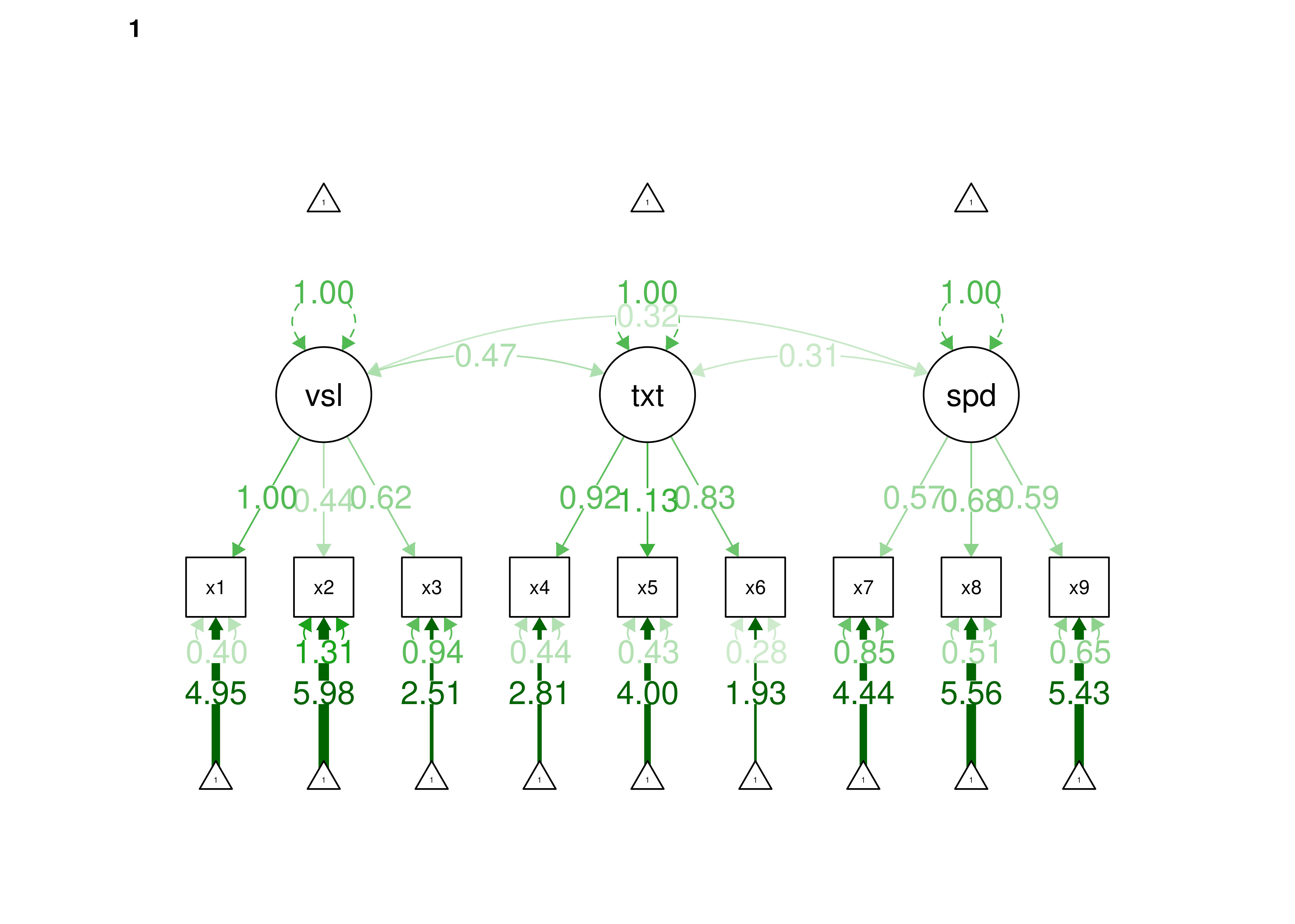
Figure 16.53: Configural Invariance Model in Confirmatory Factor Analysis (1 = Group 1; 2 = Group 2).
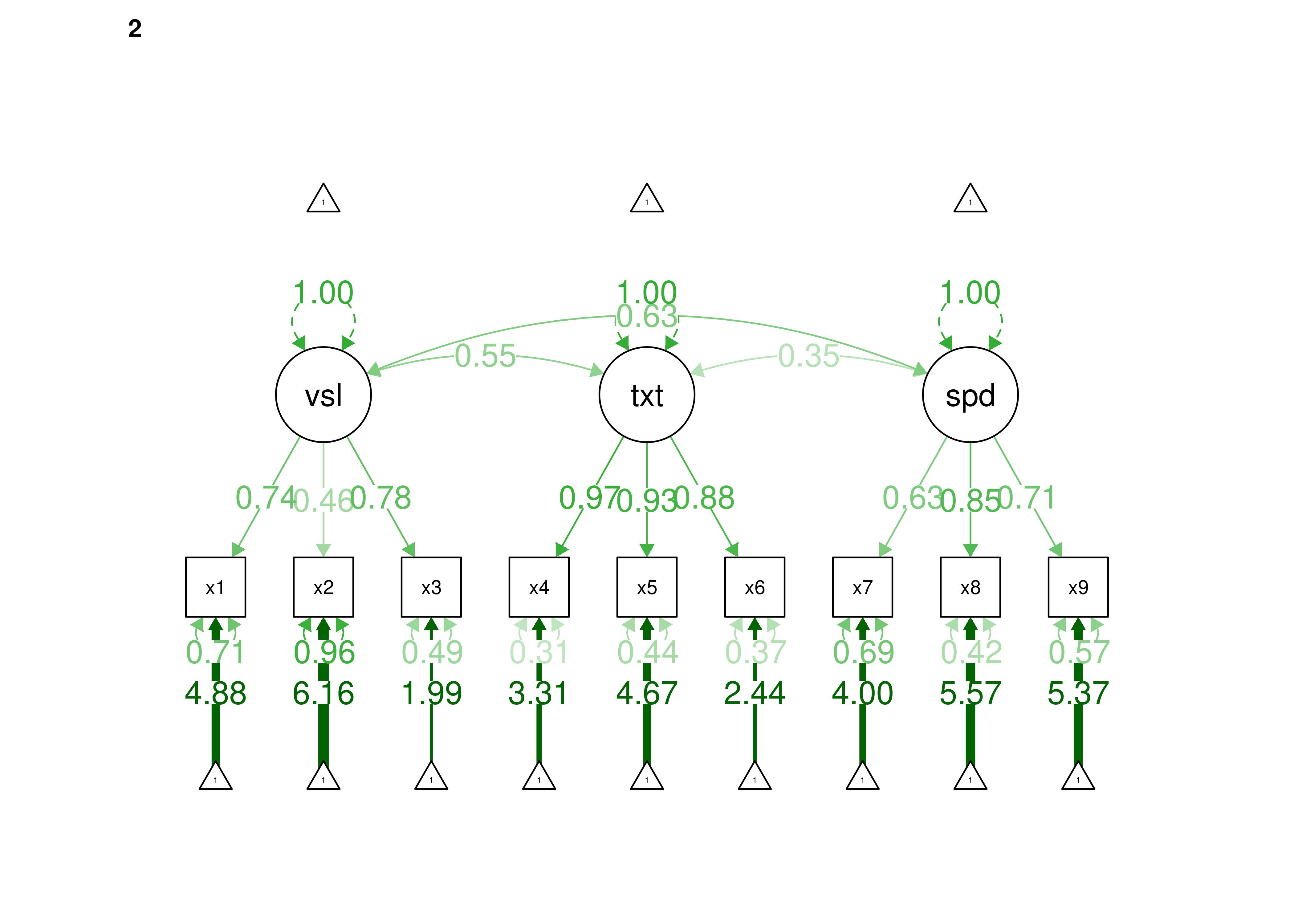
Figure 16.54: Configural Invariance Model in Confirmatory Factor Analysis (1 = Group 1; 2 = Group 2).
16.10.6 Metric (“Weak Factorial”) Invariance Model
Specify invariance of factor loadings across groups.
16.10.6.1 Model Syntax
Code
## LOADINGS:

visual =~ c(NA, NA)*x1 + c(lambda.1_1, lambda.1_1)*x1
visual =~ c(NA, NA)*x2 + c(lambda.2_1, lambda.2_1)*x2
visual =~ c(NA, NA)*x3 + c(lambda.3_1, lambda.3_1)*x3
textual =~ c(NA, NA)*x4 + c(lambda.4_2, lambda.4_2)*x4
textual =~ c(NA, NA)*x5 + c(lambda.5_2, lambda.5_2)*x5
textual =~ c(NA, NA)*x6 + c(lambda.6_2, lambda.6_2)*x6
speed =~ c(NA, NA)*x7 + c(lambda.7_3, lambda.7_3)*x7
speed =~ c(NA, NA)*x8 + c(lambda.8_3, lambda.8_3)*x8
speed =~ c(NA, NA)*x9 + c(lambda.9_3, lambda.9_3)*x9

## INTERCEPTS:

x1 ~ c(NA, NA)*1 + c(nu.1.g1, nu.1.g2)*1
x2 ~ c(NA, NA)*1 + c(nu.2.g1, nu.2.g2)*1
x3 ~ c(NA, NA)*1 + c(nu.3.g1, nu.3.g2)*1
x4 ~ c(NA, NA)*1 + c(nu.4.g1, nu.4.g2)*1
x5 ~ c(NA, NA)*1 + c(nu.5.g1, nu.5.g2)*1
x6 ~ c(NA, NA)*1 + c(nu.6.g1, nu.6.g2)*1
x7 ~ c(NA, NA)*1 + c(nu.7.g1, nu.7.g2)*1
x8 ~ c(NA, NA)*1 + c(nu.8.g1, nu.8.g2)*1
x9 ~ c(NA, NA)*1 + c(nu.9.g1, nu.9.g2)*1

## UNIQUE-FACTOR VARIANCES:

x1 ~~ c(NA, NA)*x1 + c(theta.1_1.g1, theta.1_1.g2)*x1
x2 ~~ c(NA, NA)*x2 + c(theta.2_2.g1, theta.2_2.g2)*x2
x3 ~~ c(NA, NA)*x3 + c(theta.3_3.g1, theta.3_3.g2)*x3
x4 ~~ c(NA, NA)*x4 + c(theta.4_4.g1, theta.4_4.g2)*x4
x5 ~~ c(NA, NA)*x5 + c(theta.5_5.g1, theta.5_5.g2)*x5
x6 ~~ c(NA, NA)*x6 + c(theta.6_6.g1, theta.6_6.g2)*x6
x7 ~~ c(NA, NA)*x7 + c(theta.7_7.g1, theta.7_7.g2)*x7
x8 ~~ c(NA, NA)*x8 + c(theta.8_8.g1, theta.8_8.g2)*x8
x9 ~~ c(NA, NA)*x9 + c(theta.9_9.g1, theta.9_9.g2)*x9

## LATENT MEANS/INTERCEPTS:

visual ~ c(0, 0)*1 + c(alpha.1.g1, alpha.1.g2)*1
textual ~ c(0, 0)*1 + c(alpha.2.g1, alpha.2.g2)*1
speed ~ c(0, 0)*1 + c(alpha.3.g1, alpha.3.g2)*1

## COMMON-FACTOR VARIANCES:

visual ~~ c(1, NA)*visual + c(psi.1_1.g1, psi.1_1.g2)*visual
textual ~~ c(1, NA)*textual + c(psi.2_2.g1, psi.2_2.g2)*textual
speed ~~ c(1, NA)*speed + c(psi.3_3.g1, psi.3_3.g2)*speed

## COMMON-FACTOR COVARIANCES:

visual ~~ c(NA, NA)*textual + c(psi.2_1.g1, psi.2_1.g2)*textual
visual ~~ c(NA, NA)*speed + c(psi.3_1.g1, psi.3_1.g2)*speed
textual ~~ c(NA, NA)*speed + c(psi.3_2.g1, psi.3_2.g2)*speed16.10.6.1.1 Summary of Model Features
This lavaan model syntax specifies a CFA with 9 manifest indicators of 3 common factor(s).

To identify the location and scale of each common factor, the factor means and variances were fixed to 0 and 1, respectively, unless equality constraints on measurement parameters allow them to be freed.

Pattern matrix indicating num(eric), ord(ered), and lat(ent) indicators per factor:

   visual textual speed
x1 num
x2 num
x3 num
x4        num
x5        num
x6        num
x7                num
x8                num
x9                num

The following types of parameter were constrained to equality across groups:

loadings16.10.6.4 Model Summary
lavaan 0.6-20 ended normally after 73 iterations

  Estimator                                         ML
  Optimization method                           NLMINB
  Number of model parameters                        63
  Number of equality constraints                     9

  Number of observations per group:
    Pasteur                                        156
    Grant-White                                    145
  Number of missing patterns per group:
    Pasteur                                          9
    Grant-White                                      9

Model Test User Model:
                                              Standard      Scaled
  Test Statistic                               116.313     117.955
  Degrees of freedom                                54          54
  P-value (Chi-square)                           0.000       0.000
  Scaling correction factor                                  0.986
    Yuan-Bentler correction (Mplus variant)
  Test statistic for each group:
    Pasteur                                     64.366      64.366
    Grant-White                                 53.590      53.590

Model Test Baseline Model:

  Test statistic                               932.665     909.019
  Degrees of freedom                                72          72
  P-value                                        0.000       0.000
  Scaling correction factor                                  1.026

User Model versus Baseline Model:

  Comparative Fit Index (CFI)                    0.928       0.924
  Tucker-Lewis Index (TLI)                       0.903       0.898

  Robust Comparative Fit Index (CFI)                         0.928
  Robust Tucker-Lewis Index (TLI)                            0.905

Loglikelihood and Information Criteria:

  Loglikelihood user model (H0)              -3652.277   -3652.277
  Scaling correction factor                                  0.928
      for the MLR correction
  Loglikelihood unrestricted model (H1)      -3594.120   -3594.120
  Scaling correction factor                                  1.034
      for the MLR correction

  Akaike (AIC)                                7412.554    7412.554
  Bayesian (BIC)                              7612.738    7612.738
  Sample-size adjusted Bayesian (SABIC)       7441.480    7441.480

Root Mean Square Error of Approximation:

  RMSEA                                          0.088       0.089
  90 Percent confidence interval - lower         0.066       0.067
  90 Percent confidence interval - upper         0.109       0.111
  P-value H_0: RMSEA <= 0.050                    0.004       0.003
  P-value H_0: RMSEA >= 0.080                    0.730       0.757

  Robust RMSEA                                               0.088
  90 Percent confidence interval - lower                     0.066
  90 Percent confidence interval - upper                     0.111
  P-value H_0: Robust RMSEA <= 0.050                         0.004
  P-value H_0: Robust RMSEA >= 0.080                         0.740

Standardized Root Mean Square Residual:

  SRMR                                           0.069       0.069

Parameter Estimates:

  Standard errors                             Sandwich
  Information bread                           Observed
  Observed information based on                Hessian


Group 1 [Pasteur]:

Latent Variables:
                   Estimate  Std.Err  z-value  P(>|z|)   Std.lv  Std.all
  visual =~
    x1      (l.1_)    0.885    0.122    7.258    0.000    0.885    0.759
    x2      (l.2_)    0.536    0.088    6.106    0.000    0.536    0.432
    x3      (l.3_)    0.707    0.087    8.148    0.000    0.707    0.608
  textual =~
    x4      (l.4_)    0.935    0.072   12.929    0.000    0.935    0.813
    x5      (l.5_)    1.045    0.076   13.740    0.000    1.045    0.832
    x6      (l.6_)    0.874    0.070   12.496    0.000    0.874    0.865
  speed =~
    x7      (l.7_)    0.550    0.075    7.346    0.000    0.550    0.510
    x8      (l.8_)    0.675    0.087    7.784    0.000    0.675    0.686
    x9      (l.9_)    0.602    0.088    6.867    0.000    0.602    0.603

Covariances:
                   Estimate  Std.Err  z-value  P(>|z|)   Std.lv  Std.all
  visual ~~
    textul  (p.2_)    0.473    0.105    4.484    0.000    0.473    0.473
    speed  (p.3_1)    0.347    0.125    2.778    0.005    0.347    0.347
  textual ~~
    speed  (p.3_2)    0.320    0.096    3.342    0.001    0.320    0.320

Intercepts:
                   Estimate  Std.Err  z-value  P(>|z|)   Std.lv  Std.all
   .x1      (n.1.)    4.948    0.095   52.314    0.000    4.948    4.243
   .x2      (n.2.)    5.984    0.098   60.949    0.000    5.984    4.823
   .x3      (n.3.)    2.510    0.093   26.891    0.000    2.510    2.157
   .x4      (n.4.)    2.814    0.091   30.886    0.000    2.814    2.448
   .x5      (n.5.)    4.002    0.105   38.265    0.000    4.002    3.186
   .x6      (n.6.)    1.929    0.079   24.377    0.000    1.929    1.907
   .x7      (n.7.)    4.439    0.087   51.128    0.000    4.439    4.117
   .x8      (n.8.)    5.564    0.079   70.170    0.000    5.564    5.655
   .x9      (n.9.)    5.426    0.080   67.539    0.000    5.426    5.435
    visual  (a.1.)    0.000                               0.000    0.000
    textual (a.2.)    0.000                               0.000    0.000
    speed   (a.3.)    0.000                               0.000    0.000

Variances:
                   Estimate  Std.Err  z-value  P(>|z|)   Std.lv  Std.all
   .x1      (t.1_)    0.577    0.166    3.482    0.000    0.577    0.424
   .x2      (t.2_)    1.252    0.162    7.718    0.000    1.252    0.813
   .x3      (t.3_)    0.853    0.127    6.737    0.000    0.853    0.630
   .x4      (t.4_)    0.447    0.072    6.189    0.000    0.447    0.339
   .x5      (t.5_)    0.486    0.075    6.445    0.000    0.486    0.308
   .x6      (t.6_)    0.258    0.057    4.499    0.000    0.258    0.252
   .x7      (t.7_)    0.860    0.114    7.549    0.000    0.860    0.739
   .x8      (t.8_)    0.512    0.097    5.296    0.000    0.512    0.529
   .x9      (t.9_)    0.635    0.118    5.376    0.000    0.635    0.637
    visual  (p.1_)    1.000                               1.000    1.000
    textual (p.2_)    1.000                               1.000    1.000
    speed   (p.3_)    1.000                               1.000    1.000

R-Square:
                   Estimate
    x1                0.576
    x2                0.187
    x3                0.370
    x4                0.661
    x5                0.692
    x6                0.748
    x7                0.261
    x8                0.471
    x9                0.363


Group 2 [Grant-White]:

Latent Variables:
                   Estimate  Std.Err  z-value  P(>|z|)   Std.lv  Std.all
  visual =~
    x1      (l.1_)    0.885    0.122    7.258    0.000    0.844    0.723
    x2      (l.2_)    0.536    0.088    6.106    0.000    0.512    0.467
    x3      (l.3_)    0.707    0.087    8.148    0.000    0.675    0.655
  textual =~
    x4      (l.4_)    0.935    0.072   12.929    0.000    0.937    0.846
    x5      (l.5_)    1.045    0.076   13.740    0.000    1.047    0.864
    x6      (l.6_)    0.874    0.070   12.496    0.000    0.876    0.798
  speed =~
    x7      (l.7_)    0.550    0.075    7.346    0.000    0.674    0.649
    x8      (l.8_)    0.675    0.087    7.784    0.000    0.826    0.790
    x9      (l.9_)    0.602    0.088    6.867    0.000    0.736    0.719

Covariances:
                   Estimate  Std.Err  z-value  P(>|z|)   Std.lv  Std.all
  visual ~~
    textul  (p.2_)    0.520    0.134    3.867    0.000    0.544    0.544
    speed  (p.3_1)    0.638    0.211    3.023    0.002    0.546    0.546
  textual ~~
    speed  (p.3_2)    0.429    0.193    2.219    0.026    0.350    0.350

Intercepts:
                   Estimate  Std.Err  z-value  P(>|z|)   Std.lv  Std.all
   .x1      (n.1.)    4.930    0.096   51.453    0.000    4.930    4.220
   .x2      (n.2.)    6.198    0.092   67.063    0.000    6.198    5.654
   .x3      (n.3.)    1.992    0.086   23.042    0.000    1.992    1.934
   .x4      (n.4.)    3.318    0.093   35.501    0.000    3.318    2.997
   .x5      (n.5.)    4.714    0.097   48.693    0.000    4.714    3.891
   .x6      (n.6.)    2.467    0.094   26.165    0.000    2.467    2.246
   .x7      (n.7.)    3.923    0.087   45.299    0.000    3.923    3.782
   .x8      (n.8.)    5.488    0.087   63.174    0.000    5.488    5.250
   .x9      (n.9.)    5.338    0.085   62.628    0.000    5.338    5.216
    visual  (a.1.)    0.000                               0.000    0.000
    textual (a.2.)    0.000                               0.000    0.000
    speed   (a.3.)    0.000                               0.000    0.000

Variances:
                   Estimate  Std.Err  z-value  P(>|z|)   Std.lv  Std.all
   .x1      (t.1_)    0.652    0.168    3.877    0.000    0.652    0.478
   .x2      (t.2_)    0.940    0.145    6.473    0.000    0.940    0.782
   .x3      (t.3_)    0.606    0.113    5.376    0.000    0.606    0.571
   .x4      (t.4_)    0.348    0.066    5.257    0.000    0.348    0.284
   .x5      (t.5_)    0.371    0.074    5.021    0.000    0.371    0.253
   .x6      (t.6_)    0.439    0.076    5.738    0.000    0.439    0.364
   .x7      (t.7_)    0.622    0.098    6.338    0.000    0.622    0.578
   .x8      (t.8_)    0.410    0.148    2.765    0.006    0.410    0.375
   .x9      (t.9_)    0.505    0.128    3.957    0.000    0.505    0.482
    visual  (p.1_)    0.910    0.234    3.895    0.000    1.000    1.000
    textual (p.2_)    1.004    0.191    5.257    0.000    1.000    1.000
    speed   (p.3_)    1.498    0.357    4.201    0.000    1.000    1.000

R-Square:
                   Estimate
    x1                0.522
    x2                0.218
    x3                0.429
    x4                0.716
    x5                0.747
    x6                0.636
    x7                0.422
    x8                0.625
    x9                0.518
Code
lavaan 0.6-20 ended normally after 73 iterations

  Estimator                                         ML
  Optimization method                           NLMINB
  Number of model parameters                        63
  Number of equality constraints                     9

  Number of observations per group:
    Pasteur                                        156
    Grant-White                                    145
  Number of missing patterns per group:
    Pasteur                                          9
    Grant-White                                      9

Model Test User Model:
                                              Standard      Scaled
  Test Statistic                               116.313     117.955
  Degrees of freedom                                54          54
  P-value (Chi-square)                           0.000       0.000
  Scaling correction factor                                  0.986
    Yuan-Bentler correction (Mplus variant)
  Test statistic for each group:
    Pasteur                                     64.366      64.366
    Grant-White                                 53.590      53.590

Model Test Baseline Model:

  Test statistic                               932.665     909.019
  Degrees of freedom                                72          72
  P-value                                        0.000       0.000
  Scaling correction factor                                  1.026

User Model versus Baseline Model:

  Comparative Fit Index (CFI)                    0.928       0.924
  Tucker-Lewis Index (TLI)                       0.903       0.898

  Robust Comparative Fit Index (CFI)                         0.928
  Robust Tucker-Lewis Index (TLI)                            0.905

Loglikelihood and Information Criteria:

  Loglikelihood user model (H0)              -3652.277   -3652.277
  Scaling correction factor                                  0.928
      for the MLR correction
  Loglikelihood unrestricted model (H1)      -3594.120   -3594.120
  Scaling correction factor                                  1.034
      for the MLR correction

  Akaike (AIC)                                7412.554    7412.554
  Bayesian (BIC)                              7612.738    7612.738
  Sample-size adjusted Bayesian (SABIC)       7441.480    7441.480

Root Mean Square Error of Approximation:

  RMSEA                                          0.088       0.089
  90 Percent confidence interval - lower         0.066       0.067
  90 Percent confidence interval - upper         0.109       0.111
  P-value H_0: RMSEA <= 0.050                    0.004       0.003
  P-value H_0: RMSEA >= 0.080                    0.730       0.757

  Robust RMSEA                                               0.088
  90 Percent confidence interval - lower                     0.066
  90 Percent confidence interval - upper                     0.111
  P-value H_0: Robust RMSEA <= 0.050                         0.004
  P-value H_0: Robust RMSEA >= 0.080                         0.740

Standardized Root Mean Square Residual:

  SRMR                                           0.069       0.069

Parameter Estimates:

  Standard errors                             Sandwich
  Information bread                           Observed
  Observed information based on                Hessian


Group 1 [Pasteur]:

Latent Variables:
                   Estimate  Std.Err  z-value  P(>|z|)   Std.lv  Std.all
  visual =~
    x1      (lmb1)    0.885    0.122    7.258    0.000    0.885    0.759
    x2      (lmb2)    0.536    0.088    6.106    0.000    0.536    0.432
    x3      (lmb3)    0.707    0.087    8.148    0.000    0.707    0.608
  textual =~
    x4      (lmb4)    0.935    0.072   12.929    0.000    0.935    0.813
    x5      (lmb5)    1.045    0.076   13.740    0.000    1.045    0.832
    x6      (lmb6)    0.874    0.070   12.496    0.000    0.874    0.865
  speed =~
    x7      (lmb7)    0.550    0.075    7.346    0.000    0.550    0.510
    x8      (lmb8)    0.675    0.087    7.784    0.000    0.675    0.686
    x9      (lmb9)    0.602    0.088    6.867    0.000    0.602    0.603

Covariances:
                   Estimate  Std.Err  z-value  P(>|z|)   Std.lv  Std.all
  visual ~~
    textual           0.473    0.105    4.484    0.000    0.473    0.473
    speed             0.347    0.125    2.778    0.005    0.347    0.347
  textual ~~
    speed             0.320    0.096    3.342    0.001    0.320    0.320

Intercepts:
                   Estimate  Std.Err  z-value  P(>|z|)   Std.lv  Std.all
    visual            0.000                               0.000    0.000
    textual           0.000                               0.000    0.000
    speed             0.000                               0.000    0.000
   .x1                4.948    0.095   52.314    0.000    4.948    4.243
   .x2                5.984    0.098   60.949    0.000    5.984    4.823
   .x3                2.510    0.093   26.891    0.000    2.510    2.157
   .x4                2.814    0.091   30.886    0.000    2.814    2.448
   .x5                4.002    0.105   38.265    0.000    4.002    3.186
   .x6                1.929    0.079   24.377    0.000    1.929    1.907
   .x7                4.439    0.087   51.128    0.000    4.439    4.117
   .x8                5.564    0.079   70.170    0.000    5.564    5.655
   .x9                5.426    0.080   67.539    0.000    5.426    5.435

Variances:
                   Estimate  Std.Err  z-value  P(>|z|)   Std.lv  Std.all
    visual            1.000                               1.000    1.000
    textual           1.000                               1.000    1.000
    speed             1.000                               1.000    1.000
   .x1                0.577    0.166    3.482    0.000    0.577    0.424
   .x2                1.252    0.162    7.718    0.000    1.252    0.813
   .x3                0.853    0.127    6.737    0.000    0.853    0.630
   .x4                0.447    0.072    6.189    0.000    0.447    0.339
   .x5                0.486    0.075    6.445    0.000    0.486    0.308
   .x6                0.258    0.057    4.499    0.000    0.258    0.252
   .x7                0.860    0.114    7.549    0.000    0.860    0.739
   .x8                0.512    0.097    5.296    0.000    0.512    0.529
   .x9                0.635    0.118    5.376    0.000    0.635    0.637

R-Square:
                   Estimate
    x1                0.576
    x2                0.187
    x3                0.370
    x4                0.661
    x5                0.692
    x6                0.748
    x7                0.261
    x8                0.471
    x9                0.363


Group 2 [Grant-White]:

Latent Variables:
                   Estimate  Std.Err  z-value  P(>|z|)   Std.lv  Std.all
  visual =~
    x1      (lmb1)    0.885    0.122    7.258    0.000    0.844    0.723
    x2      (lmb2)    0.536    0.088    6.106    0.000    0.512    0.467
    x3      (lmb3)    0.707    0.087    8.148    0.000    0.675    0.655
  textual =~
    x4      (lmb4)    0.935    0.072   12.929    0.000    0.937    0.846
    x5      (lmb5)    1.045    0.076   13.740    0.000    1.047    0.864
    x6      (lmb6)    0.874    0.070   12.496    0.000    0.876    0.798
  speed =~
    x7      (lmb7)    0.550    0.075    7.346    0.000    0.674    0.649
    x8      (lmb8)    0.675    0.087    7.784    0.000    0.826    0.790
    x9      (lmb9)    0.602    0.088    6.867    0.000    0.736    0.719

Covariances:
                   Estimate  Std.Err  z-value  P(>|z|)   Std.lv  Std.all
  visual ~~
    textual           0.520    0.134    3.867    0.000    0.544    0.544
    speed             0.638    0.211    3.023    0.002    0.546    0.546
  textual ~~
    speed             0.429    0.193    2.219    0.026    0.350    0.350

Intercepts:
                   Estimate  Std.Err  z-value  P(>|z|)   Std.lv  Std.all
    visual            0.000                               0.000    0.000
    textual           0.000                               0.000    0.000
    speed             0.000                               0.000    0.000
   .x1                4.930    0.096   51.453    0.000    4.930    4.220
   .x2                6.198    0.092   67.063    0.000    6.198    5.654
   .x3                1.992    0.086   23.042    0.000    1.992    1.934
   .x4                3.318    0.093   35.501    0.000    3.318    2.997
   .x5                4.714    0.097   48.693    0.000    4.714    3.891
   .x6                2.467    0.094   26.165    0.000    2.467    2.246
   .x7                3.923    0.087   45.299    0.000    3.923    3.782
   .x8                5.488    0.087   63.174    0.000    5.488    5.250
   .x9                5.338    0.085   62.628    0.000    5.338    5.216

Variances:
                   Estimate  Std.Err  z-value  P(>|z|)   Std.lv  Std.all
    visual            0.910    0.234    3.895    0.000    1.000    1.000
    textual           1.004    0.191    5.257    0.000    1.000    1.000
    speed             1.498    0.357    4.201    0.000    1.000    1.000
   .x1                0.652    0.168    3.877    0.000    0.652    0.478
   .x2                0.940    0.145    6.473    0.000    0.940    0.782
   .x3                0.606    0.113    5.376    0.000    0.606    0.571
   .x4                0.348    0.066    5.257    0.000    0.348    0.284
   .x5                0.371    0.074    5.021    0.000    0.371    0.253
   .x6                0.439    0.076    5.738    0.000    0.439    0.364
   .x7                0.622    0.098    6.338    0.000    0.622    0.578
   .x8                0.410    0.148    2.765    0.006    0.410    0.375
   .x9                0.505    0.128    3.957    0.000    0.505    0.482

R-Square:
                   Estimate
    x1                0.522
    x2                0.218
    x3                0.429
    x4                0.716
    x5                0.747
    x6                0.636
    x7                0.422
    x8                0.625
    x9                0.518
16.10.6.5 Model Fit
You can specify the null model as the baseline model using: baseline.model = nullModelFit
                         npar                          fmin
                       54.000                         0.193
                        chisq                            df
                      116.313                        54.000
                       pvalue                  chisq.scaled
                        0.000                       117.955
                    df.scaled                 pvalue.scaled
                       54.000                         0.000
         chisq.scaling.factor                baseline.chisq
                        0.986                       932.665
                  baseline.df               baseline.pvalue
                       72.000                         0.000
        baseline.chisq.scaled            baseline.df.scaled
                      909.019                        72.000
       baseline.pvalue.scaled baseline.chisq.scaling.factor
                        0.000                         1.026
                          cfi                           tli
                        0.928                         0.903
                   cfi.scaled                    tli.scaled
                        0.924                         0.898
                   cfi.robust                    tli.robust
                        0.928                         0.905
                         nnfi                           rfi
                        0.903                         0.834
                          nfi                          pnfi
                        0.875                         0.656
                          ifi                           rni
                        0.929                         0.928
                  nnfi.scaled                    rfi.scaled
                        0.898                         0.827
                   nfi.scaled                   pnfi.scaled
                        0.870                         0.653
                   ifi.scaled                    rni.scaled
                        0.925                         0.924
                  nnfi.robust                    rni.robust
                        0.905                         0.928
                         logl             unrestricted.logl
                    -3652.277                     -3594.120
                          aic                           bic
                     7412.554                      7612.738
                       ntotal                          bic2
                      301.000                      7441.480
            scaling.factor.h1             scaling.factor.h0
                        1.034                         0.928
                        rmsea                rmsea.ci.lower
                        0.088                         0.066
               rmsea.ci.upper                rmsea.ci.level
                        0.109                         0.900
                 rmsea.pvalue                rmsea.close.h0
                        0.004                         0.050
        rmsea.notclose.pvalue             rmsea.notclose.h0
                        0.730                         0.080
                 rmsea.scaled         rmsea.ci.lower.scaled
                        0.089                         0.067
        rmsea.ci.upper.scaled           rmsea.pvalue.scaled
                        0.111                         0.003
 rmsea.notclose.pvalue.scaled                  rmsea.robust
                        0.757                         0.088
        rmsea.ci.lower.robust         rmsea.ci.upper.robust
                        0.066                         0.111
          rmsea.pvalue.robust  rmsea.notclose.pvalue.robust
                        0.004                         0.740
                          rmr                    rmr_nomean
                        0.085                         0.093
                         srmr                  srmr_bentler
                        0.069                         0.069
          srmr_bentler_nomean                          crmr
                        0.075                         0.073
                  crmr_nomean                    srmr_mplus
                        0.081                         0.072
            srmr_mplus_nomean                         cn_05
                        0.074                       187.721
                        cn_01                           gfi
                      210.793                         0.995
                         agfi                          pgfi
                        0.989                         0.497
                          mfi                          ecvi
                        0.902                         0.745
Code
metricInvarianceModelFitIndices <- fitMeasures(
  metricInvarianceModel_fit)[c(
    "cfi.robust", "rmsea.robust", "srmr")]

metricInvarianceModel_chisquare <- fitMeasures(
  metricInvarianceModel_fit)[c("chisq.scaled")]

metricInvarianceModel_chisquareScaling <- fitMeasures(
  metricInvarianceModel_fit)[c("chisq.scaling.factor")]

metricInvarianceModel_df <- fitMeasures(
  metricInvarianceModel_fit)[c("df.scaled")]

metricInvarianceModel_N <- lavInspect(
  metricInvarianceModel_fit, what = "ntotal")
16.10.6.6 Compare Model Fit
16.10.6.6.1 Nested Model (\(\chi^2\)) Difference Test
The configural invariance model and the metric (“weak factorial”) invariance model are considered “nested” models. The metric invariance model is nested within the configural invariance model because the configural invariance model includes all of the terms of the metric invariance model along with additional terms. Model fit of nested models can be compared with a chi-square difference test, also known as a likelihood ratio test or deviance test. A significant chi-square difference test would indicate that the simplified model with additional constraints (the metric invariance model) is significantly worse fitting than the more complex model that has fewer constraints (the configural invariance model).
The metric invariance model did not fit significantly worse than the configural invariance model, so metric invariance held. This provides evidence of measurement invariance of factor loadings across groups. Measurement invariance of factor loadings across groups provides support for examining whether the groups show different associations of the factor with other constructs (Little et al., 2007).
The petersenlab package (Petersen, 2025) contains the satorraBentlerScaledChiSquareDifferenceTestStatistic() function that performs a Satorra-Bentler scaled chi-square difference test:
Below is a Satorra-Bentler scaled chi-square difference test, where \(c0\) and \(c1\) are the scaling correction factor for the nested model and comparison model, respectively; \(d0\) and \(d1\) are the degrees of freedom of the nested model and comparison model, respectively; and \(T0\) and \(T1\) are the chi-square values of the nested model and comparison model, respectively.
Code
metricInvarianceModel_chisquareDiff <-
  satorraBentlerScaledChiSquareDifferenceTestStatistic(
    T0 = metricInvarianceModel_chisquare,
    c0 = metricInvarianceModel_chisquareScaling,
    d0 = metricInvarianceModel_df,
    T1 = configuralInvarianceModel_chisquare,
    c1 = configuralInvarianceModel_chisquareScaling,
    d1 = configuralInvarianceModel_df)

metricInvarianceModel_chisquareDiff
chisq.scaled
5.464443 16.10.6.6.3 Score-Based Test
Score-based tests of measurement invariance are implemented using the strucchange package and are described by T. Wang et al. (2014).
  lambda.1_1   lambda.2_1   lambda.3_1   lambda.4_2   lambda.5_2   lambda.6_2
       0.885        0.536        0.707        0.935        1.045        0.874
  lambda.7_3   lambda.8_3   lambda.9_3      nu.1.g1      nu.2.g1      nu.3.g1
       0.550        0.675        0.602        4.948        5.984        2.510
     nu.4.g1      nu.5.g1      nu.6.g1      nu.7.g1      nu.8.g1      nu.9.g1
       2.814        4.002        1.929        4.439        5.564        5.426
theta.1_1.g1 theta.2_2.g1 theta.3_3.g1 theta.4_4.g1 theta.5_5.g1 theta.6_6.g1
       0.577        1.252        0.853        0.447        0.486        0.258
theta.7_7.g1 theta.8_8.g1 theta.9_9.g1   psi.2_1.g1   psi.3_1.g1   psi.3_2.g1
       0.860        0.512        0.635        0.473        0.347        0.320
  lambda.1_1   lambda.2_1   lambda.3_1   lambda.4_2   lambda.5_2   lambda.6_2
       0.885        0.536        0.707        0.935        1.045        0.874
  lambda.7_3   lambda.8_3   lambda.9_3      nu.1.g2      nu.2.g2      nu.3.g2
       0.550        0.675        0.602        4.930        6.198        1.992
     nu.4.g2      nu.5.g2      nu.6.g2      nu.7.g2      nu.8.g2      nu.9.g2
       3.318        4.714        2.467        3.923        5.488        5.338
theta.1_1.g2 theta.2_2.g2 theta.3_3.g2 theta.4_4.g2 theta.5_5.g2 theta.6_6.g2
       0.652        0.940        0.606        0.348        0.371        0.439
theta.7_7.g2 theta.8_8.g2 theta.9_9.g2   psi.1_1.g2   psi.2_2.g2   psi.3_3.g2
       0.622        0.410        0.505        0.910        1.004        1.498
  psi.2_1.g2   psi.3_1.g2   psi.3_2.g2
0.520 0.638 0.429 lambda.1_1 lambda.2_1 lambda.3_1 lambda.4_2 lambda.5_2 lambda.6_2 lambda.7_3
0.8850052 0.5363099 0.7072357 0.9347277 1.0449934 0.8743059 0.5504042
lambda.8_3 lambda.9_3
0.6751277 0.6015120 Code
    M-fluctuation test

data:  metricInvarianceModel_fit
f(efp) = 5.0601, p-value = 0.829
A score-based test and expected parameter change (EPC) estimates (Oberski, 2014; Oberski et al., 2015) are provided by the lavaan package (Rosseel et al., 2022).
$test

total score test:

   test    X2 df p.value
1 score 6.199  9    0.72

$uni

univariate score tests:

   lhs op   rhs    X2 df p.value
1 .p1. == .p37. 1.303  1   0.254
2 .p2. == .p38. 0.468  1   0.494
3 .p3. == .p39. 0.334  1   0.563
4 .p4. == .p40. 0.314  1   0.575
5 .p5. == .p41. 4.447  1   0.035
6 .p6. == .p42. 2.539  1   0.111
7 .p7. == .p43. 0.027  1   0.869
8 .p8. == .p44. 0.005  1   0.942
9 .p9. == .p45. 0.007  1   0.932

$epc

expected parameter changes (epc) and expected parameter values (epv):

       lhs op     rhs block group free        label plabel   est    epc   epv
1   visual =~      x1     1     1    1   lambda.1_1   .p1. 0.885  0.072 0.957
2   visual =~      x2     1     1    2   lambda.2_1   .p2. 0.536 -0.060 0.476
3   visual =~      x3     1     1    3   lambda.3_1   .p3. 0.707 -0.052 0.655
4  textual =~      x4     1     1    4   lambda.4_2   .p4. 0.935 -0.018 0.916
5  textual =~      x5     1     1    5   lambda.5_2   .p5. 1.045  0.081 1.126
6  textual =~      x6     1     1    6   lambda.6_2   .p6. 0.874 -0.042 0.832
7    speed =~      x7     1     1    7   lambda.7_3   .p7. 0.550  0.013 0.563
8    speed =~      x8     1     1    8   lambda.8_3   .p8. 0.675 -0.004 0.671
9    speed =~      x9     1     1    9   lambda.9_3   .p9. 0.602 -0.004 0.597
10      x1 ~1             1     1   10      nu.1.g1  .p10. 4.948  0.000 4.948
11      x2 ~1             1     1   11      nu.2.g1  .p11. 5.984  0.000 5.984
12      x3 ~1             1     1   12      nu.3.g1  .p12. 2.510  0.000 2.510
13      x4 ~1             1     1   13      nu.4.g1  .p13. 2.814  0.000 2.814
14      x5 ~1             1     1   14      nu.5.g1  .p14. 4.002  0.000 4.002
15      x6 ~1             1     1   15      nu.6.g1  .p15. 1.929  0.000 1.929
16      x7 ~1             1     1   16      nu.7.g1  .p16. 4.439  0.000 4.439
17      x8 ~1             1     1   17      nu.8.g1  .p17. 5.564  0.000 5.564
18      x9 ~1             1     1   18      nu.9.g1  .p18. 5.426  0.000 5.426
19      x1 ~~      x1     1     1   19 theta.1_1.g1  .p19. 0.577 -0.094 0.483
20      x2 ~~      x2     1     1   20 theta.2_2.g1  .p20. 1.252  0.029 1.280
21      x3 ~~      x3     1     1   21 theta.3_3.g1  .p21. 0.853  0.048 0.901
22      x4 ~~      x4     1     1   22 theta.4_4.g1  .p22. 0.447  0.005 0.453
23      x5 ~~      x5     1     1   23 theta.5_5.g1  .p23. 0.486 -0.048 0.439
24      x6 ~~      x6     1     1   24 theta.6_6.g1  .p24. 0.258  0.026 0.284
25      x7 ~~      x7     1     1   25 theta.7_7.g1  .p25. 0.860 -0.007 0.853
26      x8 ~~      x8     1     1   26 theta.8_8.g1  .p26. 0.512  0.004 0.516
27      x9 ~~      x9     1     1   27 theta.9_9.g1  .p27. 0.635  0.002 0.637
28  visual ~1             1     1    0   alpha.1.g1  .p28. 0.000     NA    NA
29 textual ~1             1     1    0   alpha.2.g1  .p29. 0.000     NA    NA
30   speed ~1             1     1    0   alpha.3.g1  .p30. 0.000     NA    NA
31  visual ~~  visual     1     1    0   psi.1_1.g1  .p31. 1.000     NA    NA
32 textual ~~ textual     1     1    0   psi.2_2.g1  .p32. 1.000     NA    NA
33   speed ~~   speed     1     1    0   psi.3_3.g1  .p33. 1.000     NA    NA
34  visual ~~ textual     1     1   28   psi.2_1.g1  .p34. 0.473 -0.009 0.464
35  visual ~~   speed     1     1   29   psi.3_1.g1  .p35. 0.347 -0.007 0.341
36 textual ~~   speed     1     1   30   psi.3_2.g1  .p36. 0.320  0.001 0.320
37  visual =~      x1     2     2   31   lambda.1_1  .p37. 0.885 -0.056 0.829
38  visual =~      x2     2     2   32   lambda.2_1  .p38. 0.536  0.046 0.583
39  visual =~      x3     2     2   33   lambda.3_1  .p39. 0.707  0.033 0.740
40 textual =~      x4     2     2   34   lambda.4_2  .p40. 0.935  0.023 0.958
41 textual =~      x5     2     2   35   lambda.5_2  .p41. 1.045 -0.072 0.973
42 textual =~      x6     2     2   36   lambda.6_2  .p42. 0.874  0.065 0.939
43   speed =~      x7     2     2   37   lambda.7_3  .p43. 0.550 -0.005 0.545
44   speed =~      x8     2     2   38   lambda.8_3  .p44. 0.675  0.002 0.677
45   speed =~      x9     2     2   39   lambda.9_3  .p45. 0.602  0.002 0.604
46      x1 ~1             2     2   40      nu.1.g2  .p46. 4.930  0.000 4.930
47      x2 ~1             2     2   41      nu.2.g2  .p47. 6.198  0.000 6.198
48      x3 ~1             2     2   42      nu.3.g2  .p48. 1.992  0.000 1.992
49      x4 ~1             2     2   43      nu.4.g2  .p49. 3.318  0.000 3.318
50      x5 ~1             2     2   44      nu.5.g2  .p50. 4.714  0.000 4.714
51      x6 ~1             2     2   45      nu.6.g2  .p51. 2.467  0.000 2.467
52      x7 ~1             2     2   46      nu.7.g2  .p52. 3.923  0.000 3.923
53      x8 ~1             2     2   47      nu.8.g2  .p53. 5.488  0.000 5.488
54      x9 ~1             2     2   48      nu.9.g2  .p54. 5.338  0.000 5.338
55      x1 ~~      x1     2     2   49 theta.1_1.g2  .p55. 0.652  0.051 0.702
56      x2 ~~      x2     2     2   50 theta.2_2.g2  .p56. 0.940 -0.015 0.924
57      x3 ~~      x3     2     2   51 theta.3_3.g2  .p57. 0.606 -0.022 0.584
58      x4 ~~      x4     2     2   52 theta.4_4.g2  .p58. 0.348 -0.018 0.330
59      x5 ~~      x5     2     2   53 theta.5_5.g2  .p59. 0.371  0.050 0.421
60      x6 ~~      x6     2     2   54 theta.6_6.g2  .p60. 0.439 -0.027 0.412
61      x7 ~~      x7     2     2   55 theta.7_7.g2  .p61. 0.622  0.003 0.625
62      x8 ~~      x8     2     2   56 theta.8_8.g2  .p62. 0.410 -0.002 0.408
63      x9 ~~      x9     2     2   57 theta.9_9.g2  .p63. 0.505 -0.001 0.504
64  visual ~1             2     2    0   alpha.1.g2  .p64. 0.000     NA    NA
65 textual ~1             2     2    0   alpha.2.g2  .p65. 0.000     NA    NA
66   speed ~1             2     2    0   alpha.3.g2  .p66. 0.000     NA    NA
67  visual ~~  visual     2     2   58   psi.1_1.g2  .p67. 0.910 -0.002 0.907
68 textual ~~ textual     2     2   59   psi.2_2.g2  .p68. 1.004  0.000 1.005
69   speed ~~   speed     2     2   60   psi.3_3.g2  .p69. 1.498 -0.001 1.497
70  visual ~~ textual     2     2   61   psi.2_1.g2  .p70. 0.520  0.003 0.523
71  visual ~~   speed     2     2   62   psi.3_1.g2  .p71. 0.638  0.003 0.641
72 textual ~~   speed     2     2   63   psi.3_2.g2  .p72. 0.429  0.001 0.430
   sepc.lv sepc.all sepc.nox
1    0.072    0.062    0.062
2   -0.060   -0.048   -0.048
3   -0.052   -0.045   -0.045
4   -0.018   -0.016   -0.016
5    0.081    0.065    0.065
6   -0.042   -0.042   -0.042
7    0.013    0.012    0.012
8   -0.004   -0.004   -0.004
9   -0.004   -0.004   -0.004
10   0.000    0.000    0.000
11   0.000    0.000    0.000
12   0.000    0.000    0.000
13   0.000    0.000    0.000
14   0.000    0.000    0.000
15   0.000    0.000    0.000
16   0.000    0.000    0.000
17   0.000    0.000    0.000
18   0.000    0.000    0.000
19  -0.577   -0.424   -0.424
20   1.252    0.813    0.813
21   0.853    0.630    0.630
22   0.447    0.339    0.339
23  -0.486   -0.308   -0.308
24   0.258    0.252    0.252
25  -0.860   -0.739   -0.739
26   0.512    0.529    0.529
27   0.635    0.637    0.637
28      NA       NA       NA
29      NA       NA       NA
30      NA       NA       NA
31      NA       NA       NA
32      NA       NA       NA
33      NA       NA       NA
34  -0.009   -0.009   -0.009
35  -0.007   -0.007   -0.007
36   0.001    0.001    0.001
37  -0.053   -0.045   -0.045
38   0.044    0.040    0.040
39   0.031    0.030    0.030
40   0.023    0.021    0.021
41  -0.072   -0.060   -0.060
42   0.065    0.059    0.059
43  -0.006   -0.006   -0.006
44   0.002    0.002    0.002
45   0.003    0.003    0.003
46   0.000    0.000    0.000
47   0.000    0.000    0.000
48   0.000    0.000    0.000
49   0.000    0.000    0.000
50   0.000    0.000    0.000
51   0.000    0.000    0.000
52   0.000    0.000    0.000
53   0.000    0.000    0.000
54   0.000    0.000    0.000
55   0.652    0.478    0.478
56  -0.940   -0.782   -0.782
57  -0.606   -0.571   -0.571
58  -0.348   -0.284   -0.284
59   0.371    0.253    0.253
60  -0.439   -0.364   -0.364
61   0.622    0.578    0.578
62  -0.410   -0.375   -0.375
63  -0.505   -0.482   -0.482
64      NA       NA       NA
65      NA       NA       NA
66      NA       NA       NA
67  -1.000   -1.000   -1.000
68   1.000    1.000    1.000
69  -1.000   -1.000   -1.000
70   0.003    0.003    0.003
71   0.002    0.002    0.002
72   0.000    0.000    0.000
16.10.6.6.4 Effect Size of Non-Invariance
The effect size of measurement non-invariance, as described by Nye et al. (2019), was calculated using the dmacs package (Dueber, 2019).
$DMACS
       visual   textual      speed
x1 0.01593095        NA         NA
x2 0.18201703        NA         NA
x3 0.46928939        NA         NA
x4         NA 0.4447078         NA
x5         NA 0.5774043         NA
x6         NA 0.5099205         NA
x7         NA        NA 0.48491342
x8         NA        NA 0.07411716
x9         NA        NA 0.08693423

$ItemDeltaMean
        visual   textual       speed
x1 -0.01861594        NA          NA
x2  0.21369298        NA          NA
x3 -0.51750811        NA          NA
x4          NA 0.5039787          NA
x5          NA 0.7122322          NA
x6          NA 0.5384225          NA
x7          NA        NA -0.51565293
x8          NA        NA -0.07526967
x9          NA        NA -0.08805919

$MeanDiff
    visual    textual      speed
-0.3224311  1.7546334 -0.6789818
The \(w\) and \(\Delta \text{M}_\text{C}\) indices of the effect size of measurement non-invariance, as described by Newsom (2015), were calculated using the measurementNoninvarianceEffectSize() function of the petersenlab package (Petersen, 2025).
Code
$Mc_unconstrained
[1] 0.9026906

$Mc_constrained
[1] 0.9013555

$Delta_Mc
[1] 0.001335086

$w
[1] 0.06175749
16.10.6.6.5 Equivalence Test
The petersenlab package (Petersen, 2025) contains the equiv_chi() function from Counsell et al. (2020) that performs an equivalence test: https://osf.io/cqu8v.
The chi-square equivalence test is non-significant, suggesting that the model fit is not acceptable.
Code
Moreover, the equivalence test of the chi-square difference test is non-significant, suggesting that the degree of worsening of model fit is not acceptable. In other words, metric invariance failed.
Code
16.10.6.6.6 Permutation Test
Permutation procedures for testing measurement invariance are described in (Jorgensen et al., 2018).
For reproducibility, I set the seed below.
Using the same seed will yield the same answer every time.
There is nothing special about this particular seed.
You can specify the null model as the baseline model using: baseline.model = nullModelFit.
Warning: this code takes a while to run based on \(100\) iterations.
You can reduce the number of iterations to be faster.
Code
set.seed(52242)
metricInvarianceTest <- permuteMeasEq(
  nPermute = numPermutations,
  modelType = "mgcfa",
  con = metricInvarianceModel_fit,
  uncon = configuralInvarianceModel_fit,
  AFIs = myAFIs,
  moreAFIs = moreAFIs,
  parallelType = "multicore", #only 'snow' works on Windows, but right now, it is throwing an error
iseed = 52242)Omnibus p value based on parametric chi-squared difference test:
Chisq diff Df diff Pr(>Chisq)
5.464 6.000 0.486
Omnibus p values based on nonparametric permutation method:
AFI.Difference p.value
chisq 6.888 0.57
chisq.scaled 2.986 0.59
rmsea -0.005 0.60
cfi -0.001 0.57
tli 0.011 0.61
srmr 0.003 0.71
rmsea.robust -0.005 0.61
cfi.robust -0.001 0.59
tli.robust 0.011 0.64The p-values are non-significant, indicating that the model does not fit significantly worse than the configural invariance model. In other words, metric invariance held.
16.10.6.7 Internal Consistency Reliability
Internal consistency reliability of items composing the latent factors, as quantified by omega (\(\omega\)) and average variance extracted (AVE), was estimated using the semTools package (Jorgensen et al., 2021).
16.10.6.8 Path Diagram
A path diagram of the model generated using the semPlot package (Epskamp, 2022) is below.
Code
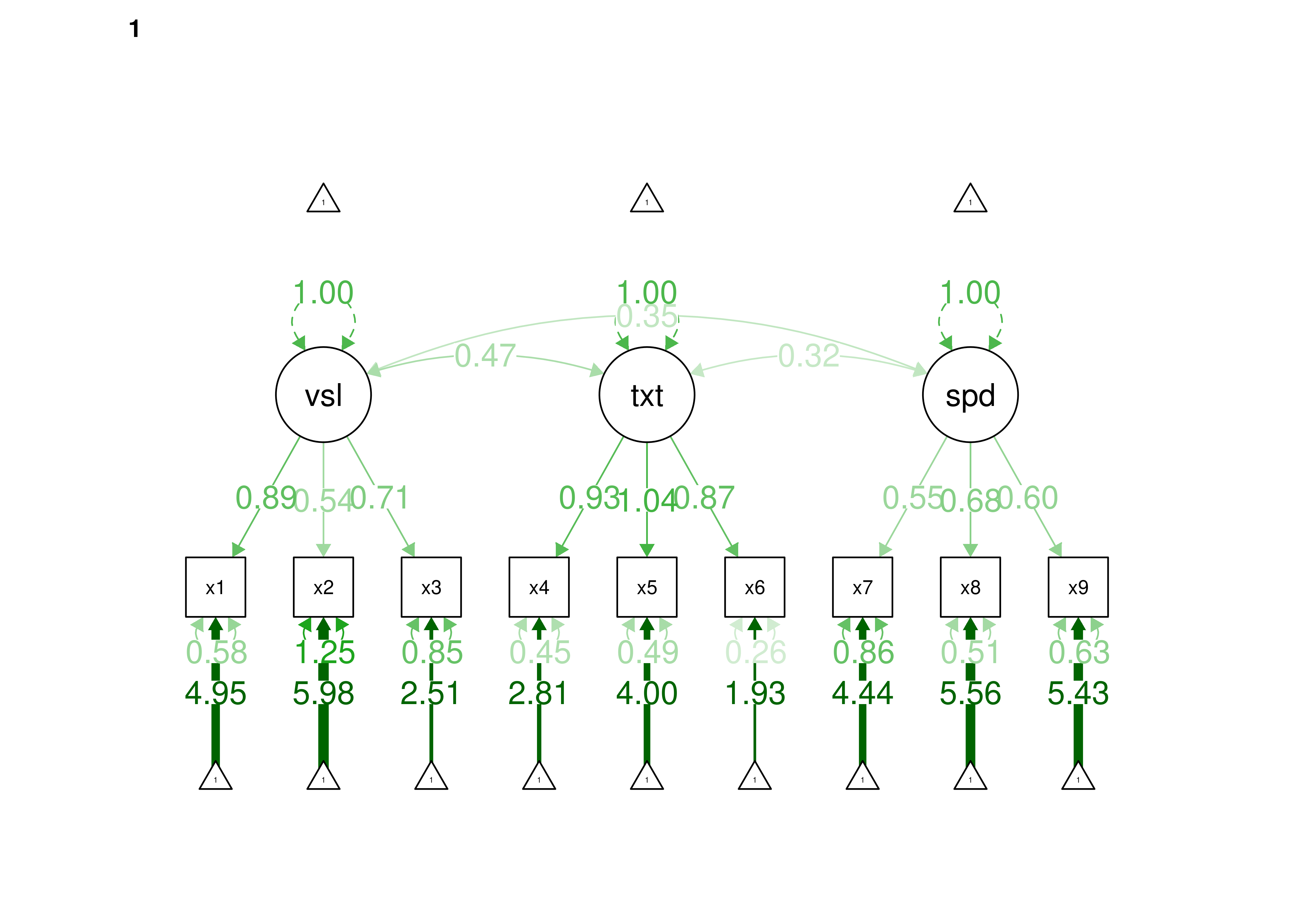
Figure 16.55: Metric Invariance Model in Confirmatory Factor Analysis.
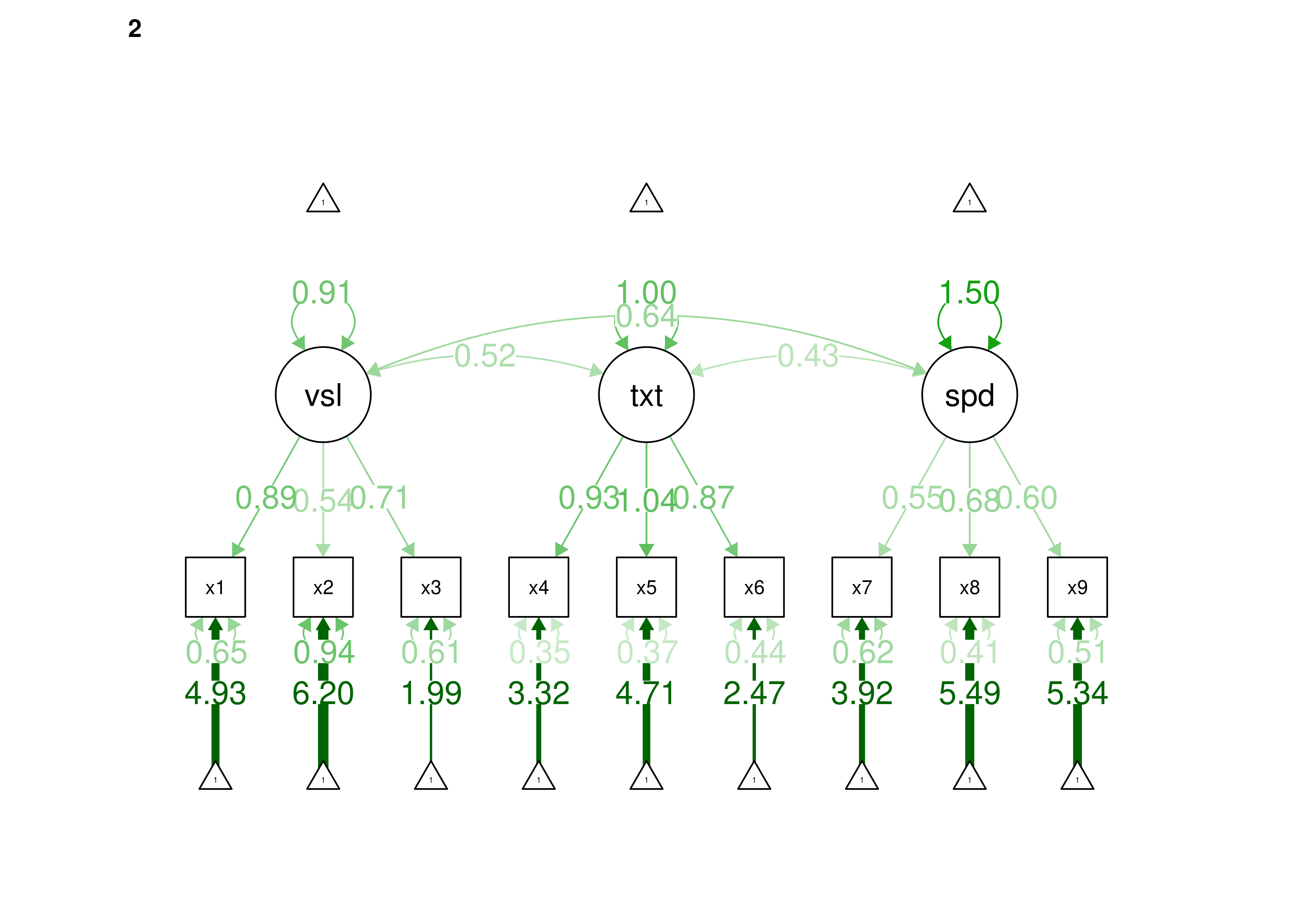
Figure 16.56: Metric Invariance Model in Confirmatory Factor Analysis.
16.10.7 Scalar (“Strong Factorial”) Invariance Model
Specify invariance of factor loadings and intercepts across groups.
16.10.7.1 Model Syntax
Code
## LOADINGS:

visual =~ c(NA, NA)*x1 + c(lambda.1_1, lambda.1_1)*x1
visual =~ c(NA, NA)*x2 + c(lambda.2_1, lambda.2_1)*x2
visual =~ c(NA, NA)*x3 + c(lambda.3_1, lambda.3_1)*x3
textual =~ c(NA, NA)*x4 + c(lambda.4_2, lambda.4_2)*x4
textual =~ c(NA, NA)*x5 + c(lambda.5_2, lambda.5_2)*x5
textual =~ c(NA, NA)*x6 + c(lambda.6_2, lambda.6_2)*x6
speed =~ c(NA, NA)*x7 + c(lambda.7_3, lambda.7_3)*x7
speed =~ c(NA, NA)*x8 + c(lambda.8_3, lambda.8_3)*x8
speed =~ c(NA, NA)*x9 + c(lambda.9_3, lambda.9_3)*x9

## INTERCEPTS:

x1 ~ c(NA, NA)*1 + c(nu.1, nu.1)*1
x2 ~ c(NA, NA)*1 + c(nu.2, nu.2)*1
x3 ~ c(NA, NA)*1 + c(nu.3, nu.3)*1
x4 ~ c(NA, NA)*1 + c(nu.4, nu.4)*1
x5 ~ c(NA, NA)*1 + c(nu.5, nu.5)*1
x6 ~ c(NA, NA)*1 + c(nu.6, nu.6)*1
x7 ~ c(NA, NA)*1 + c(nu.7, nu.7)*1
x8 ~ c(NA, NA)*1 + c(nu.8, nu.8)*1
x9 ~ c(NA, NA)*1 + c(nu.9, nu.9)*1

## UNIQUE-FACTOR VARIANCES:

x1 ~~ c(NA, NA)*x1 + c(theta.1_1.g1, theta.1_1.g2)*x1
x2 ~~ c(NA, NA)*x2 + c(theta.2_2.g1, theta.2_2.g2)*x2
x3 ~~ c(NA, NA)*x3 + c(theta.3_3.g1, theta.3_3.g2)*x3
x4 ~~ c(NA, NA)*x4 + c(theta.4_4.g1, theta.4_4.g2)*x4
x5 ~~ c(NA, NA)*x5 + c(theta.5_5.g1, theta.5_5.g2)*x5
x6 ~~ c(NA, NA)*x6 + c(theta.6_6.g1, theta.6_6.g2)*x6
x7 ~~ c(NA, NA)*x7 + c(theta.7_7.g1, theta.7_7.g2)*x7
x8 ~~ c(NA, NA)*x8 + c(theta.8_8.g1, theta.8_8.g2)*x8
x9 ~~ c(NA, NA)*x9 + c(theta.9_9.g1, theta.9_9.g2)*x9

## LATENT MEANS/INTERCEPTS:

visual ~ c(0, NA)*1 + c(alpha.1.g1, alpha.1.g2)*1
textual ~ c(0, NA)*1 + c(alpha.2.g1, alpha.2.g2)*1
speed ~ c(0, NA)*1 + c(alpha.3.g1, alpha.3.g2)*1

## COMMON-FACTOR VARIANCES:

visual ~~ c(1, NA)*visual + c(psi.1_1.g1, psi.1_1.g2)*visual
textual ~~ c(1, NA)*textual + c(psi.2_2.g1, psi.2_2.g2)*textual
speed ~~ c(1, NA)*speed + c(psi.3_3.g1, psi.3_3.g2)*speed

## COMMON-FACTOR COVARIANCES:

visual ~~ c(NA, NA)*textual + c(psi.2_1.g1, psi.2_1.g2)*textual
visual ~~ c(NA, NA)*speed + c(psi.3_1.g1, psi.3_1.g2)*speed
textual ~~ c(NA, NA)*speed + c(psi.3_2.g1, psi.3_2.g2)*speed16.10.7.1.1 Summary of Model Features
This lavaan model syntax specifies a CFA with 9 manifest indicators of 3 common factor(s).

To identify the location and scale of each common factor, the factor means and variances were fixed to 0 and 1, respectively, unless equality constraints on measurement parameters allow them to be freed.

Pattern matrix indicating num(eric), ord(ered), and lat(ent) indicators per factor:

   visual textual speed
x1 num
x2 num
x3 num
x4        num
x5        num
x6        num
x7                num
x8                num
x9                num

The following types of parameter were constrained to equality across groups:

    loadings
intercepts16.10.7.4 Model Summary
lavaan 0.6-20 ended normally after 66 iterations

  Estimator                                         ML
  Optimization method                           NLMINB
  Number of model parameters                        66
  Number of equality constraints                    18

  Number of observations per group:
    Pasteur                                        156
    Grant-White                                    145
  Number of missing patterns per group:
    Pasteur                                          9
    Grant-White                                      9

Model Test User Model:
                                              Standard      Scaled
  Test Statistic                               156.955     159.442
  Degrees of freedom                                60          60
  P-value (Chi-square)                           0.000       0.000
  Scaling correction factor                                  0.984
    Yuan-Bentler correction (Mplus variant)
  Test statistic for each group:
    Pasteur                                     86.521      86.521
    Grant-White                                 72.921      72.921

Model Test Baseline Model:

  Test statistic                               932.665     909.019
  Degrees of freedom                                72          72
  P-value                                        0.000       0.000
  Scaling correction factor                                  1.026

User Model versus Baseline Model:

  Comparative Fit Index (CFI)                    0.887       0.881
  Tucker-Lewis Index (TLI)                       0.865       0.857

  Robust Comparative Fit Index (CFI)                         0.890
  Robust Tucker-Lewis Index (TLI)                            0.868

Loglikelihood and Information Criteria:

  Loglikelihood user model (H0)              -3672.597   -3672.597
  Scaling correction factor                                  0.797
      for the MLR correction
  Loglikelihood unrestricted model (H1)      -3594.120   -3594.120
  Scaling correction factor                                  1.034
      for the MLR correction

  Akaike (AIC)                                7441.195    7441.195
  Bayesian (BIC)                              7619.136    7619.136
  Sample-size adjusted Bayesian (SABIC)       7466.908    7466.908

Root Mean Square Error of Approximation:

  RMSEA                                          0.104       0.105
  90 Percent confidence interval - lower         0.084       0.085
  90 Percent confidence interval - upper         0.124       0.125
  P-value H_0: RMSEA <= 0.050                    0.000       0.000
  P-value H_0: RMSEA >= 0.080                    0.975       0.980

  Robust RMSEA                                               0.104
  90 Percent confidence interval - lower                     0.083
  90 Percent confidence interval - upper                     0.124
  P-value H_0: Robust RMSEA <= 0.050                         0.000
  P-value H_0: Robust RMSEA >= 0.080                         0.972

Standardized Root Mean Square Residual:

  SRMR                                           0.080       0.080

Parameter Estimates:

  Standard errors                             Sandwich
  Information bread                           Observed
  Observed information based on                Hessian


Group 1 [Pasteur]:

Latent Variables:
                   Estimate  Std.Err  z-value  P(>|z|)   Std.lv  Std.all
  visual =~
    x1      (l.1_)    0.874    0.132    6.630    0.000    0.874    0.751
    x2      (l.2_)    0.512    0.086    5.984    0.000    0.512    0.411
    x3      (l.3_)    0.722    0.095    7.610    0.000    0.722    0.604
  textual =~
    x4      (l.4_)    0.921    0.071   12.920    0.000    0.921    0.807
    x5      (l.5_)    1.059    0.077   13.763    0.000    1.059    0.837
    x6      (l.6_)    0.875    0.066   13.259    0.000    0.875    0.865
  speed =~
    x7      (l.7_)    0.566    0.081    6.946    0.000    0.566    0.512
    x8      (l.8_)    0.657    0.082    8.028    0.000    0.657    0.669
    x9      (l.9_)    0.602    0.085    7.049    0.000    0.602    0.604

Covariances:
                   Estimate  Std.Err  z-value  P(>|z|)   Std.lv  Std.all
  visual ~~
    textul  (p.2_)    0.473    0.108    4.397    0.000    0.473    0.473
    speed  (p.3_1)    0.355    0.125    2.842    0.004    0.355    0.355
  textual ~~
    speed  (p.3_2)    0.322    0.095    3.377    0.001    0.322    0.322

Intercepts:
                   Estimate  Std.Err  z-value  P(>|z|)   Std.lv  Std.all
   .x1      (nu.1)    5.016    0.094   53.146    0.000    5.016    4.309
   .x2      (nu.2)    6.156    0.088   69.594    0.000    6.156    4.944
   .x3      (nu.3)    2.292    0.098   23.329    0.000    2.292    1.916
   .x4      (nu.4)    2.780    0.086   32.469    0.000    2.780    2.435
   .x5      (nu.5)    4.035    0.104   38.981    0.000    4.035    3.189
   .x6      (nu.6)    1.928    0.074   25.882    0.000    1.928    1.907
   .x7      (nu.7)    4.244    0.078   54.164    0.000    4.244    3.840
   .x8      (nu.8)    5.627    0.076   73.915    0.000    5.627    5.726
   .x9      (nu.9)    5.474    0.073   74.934    0.000    5.474    5.492
    visual  (a.1.)    0.000                               0.000    0.000
    textual (a.2.)    0.000                               0.000    0.000
    speed   (a.3.)    0.000                               0.000    0.000

Variances:
                   Estimate  Std.Err  z-value  P(>|z|)   Std.lv  Std.all
   .x1      (t.1_)    0.591    0.179    3.295    0.001    0.591    0.436
   .x2      (t.2_)    1.288    0.160    8.075    0.000    1.288    0.831
   .x3      (t.3_)    0.910    0.151    6.046    0.000    0.910    0.636
   .x4      (t.4_)    0.454    0.073    6.245    0.000    0.454    0.349
   .x5      (t.5_)    0.480    0.076    6.295    0.000    0.480    0.300
   .x6      (t.6_)    0.257    0.058    4.401    0.000    0.257    0.252
   .x7      (t.7_)    0.901    0.129    7.000    0.000    0.901    0.738
   .x8      (t.8_)    0.534    0.091    5.838    0.000    0.534    0.553
   .x9      (t.9_)    0.631    0.115    5.469    0.000    0.631    0.635
    visual  (p.1_)    1.000                               1.000    1.000
    textual (p.2_)    1.000                               1.000    1.000
    speed   (p.3_)    1.000                               1.000    1.000

R-Square:
                   Estimate
    x1                0.564
    x2                0.169
    x3                0.364
    x4                0.651
    x5                0.700
    x6                0.748
    x7                0.262
    x8                0.447
    x9                0.365


Group 2 [Grant-White]:

Latent Variables:
                   Estimate  Std.Err  z-value  P(>|z|)   Std.lv  Std.all
  visual =~
    x1      (l.1_)    0.874    0.132    6.630    0.000    0.827    0.711
    x2      (l.2_)    0.512    0.086    5.984    0.000    0.485    0.441
    x3      (l.3_)    0.722    0.095    7.610    0.000    0.684    0.649
  textual =~
    x4      (l.4_)    0.921    0.071   12.920    0.000    0.921    0.838
    x5      (l.5_)    1.059    0.077   13.763    0.000    1.059    0.869
    x6      (l.6_)    0.875    0.066   13.259    0.000    0.875    0.797
  speed =~
    x7      (l.7_)    0.566    0.081    6.946    0.000    0.692    0.651
    x8      (l.8_)    0.657    0.082    8.028    0.000    0.803    0.773
    x9      (l.9_)    0.602    0.085    7.049    0.000    0.736    0.722

Covariances:
                   Estimate  Std.Err  z-value  P(>|z|)   Std.lv  Std.all
  visual ~~
    textul  (p.2_)    0.519    0.136    3.829    0.000    0.549    0.549
    speed  (p.3_1)    0.649    0.215    3.014    0.003    0.561    0.561
  textual ~~
    speed  (p.3_2)    0.442    0.189    2.335    0.020    0.361    0.361

Intercepts:
                   Estimate  Std.Err  z-value  P(>|z|)   Std.lv  Std.all
   .x1      (nu.1)    5.016    0.094   53.146    0.000    5.016    4.312
   .x2      (nu.2)    6.156    0.088   69.594    0.000    6.156    5.602
   .x3      (nu.3)    2.292    0.098   23.329    0.000    2.292    2.177
   .x4      (nu.4)    2.780    0.086   32.469    0.000    2.780    2.529
   .x5      (nu.5)    4.035    0.104   38.981    0.000    4.035    3.312
   .x6      (nu.6)    1.928    0.074   25.882    0.000    1.928    1.756
   .x7      (nu.7)    4.244    0.078   54.164    0.000    4.244    3.990
   .x8      (nu.8)    5.627    0.076   73.915    0.000    5.627    5.412
   .x9      (nu.9)    5.474    0.073   74.934    0.000    5.474    5.370
    visual  (a.1.)   -0.193    0.175   -1.101    0.271   -0.204   -0.204
    textual (a.2.)    0.617    0.135    4.587    0.000    0.617    0.617
    speed   (a.3.)   -0.294    0.161   -1.828    0.068   -0.240   -0.240

Variances:
                   Estimate  Std.Err  z-value  P(>|z|)   Std.lv  Std.all
   .x1      (t.1_)    0.668    0.176    3.793    0.000    0.668    0.494
   .x2      (t.2_)    0.973    0.152    6.384    0.000    0.973    0.805
   .x3      (t.3_)    0.641    0.133    4.833    0.000    0.641    0.578
   .x4      (t.4_)    0.359    0.066    5.464    0.000    0.359    0.297
   .x5      (t.5_)    0.363    0.074    4.883    0.000    0.363    0.245
   .x6      (t.6_)    0.441    0.075    5.851    0.000    0.441    0.366
   .x7      (t.7_)    0.652    0.108    6.016    0.000    0.652    0.577
   .x8      (t.8_)    0.436    0.152    2.872    0.004    0.436    0.403
   .x9      (t.9_)    0.497    0.127    3.918    0.000    0.497    0.478
    visual  (p.1_)    0.896    0.235    3.816    0.000    1.000    1.000
    textual (p.2_)    1.000    0.194    5.157    0.000    1.000    1.000
    speed   (p.3_)    1.495    0.360    4.156    0.000    1.000    1.000

R-Square:
                   Estimate
    x1                0.506
    x2                0.195
    x3                0.422
    x4                0.703
    x5                0.755
    x6                0.634
    x7                0.423
    x8                0.597
    x9                0.522
Code
lavaan 0.6-20 ended normally after 66 iterations

  Estimator                                         ML
  Optimization method                           NLMINB
  Number of model parameters                        66
  Number of equality constraints                    18

  Number of observations per group:
    Pasteur                                        156
    Grant-White                                    145
  Number of missing patterns per group:
    Pasteur                                          9
    Grant-White                                      9

Model Test User Model:
                                              Standard      Scaled
  Test Statistic                               156.955     159.442
  Degrees of freedom                                60          60
  P-value (Chi-square)                           0.000       0.000
  Scaling correction factor                                  0.984
    Yuan-Bentler correction (Mplus variant)
  Test statistic for each group:
    Pasteur                                     86.520      86.520
    Grant-White                                 72.921      72.921

Model Test Baseline Model:

  Test statistic                               932.665     909.019
  Degrees of freedom                                72          72
  P-value                                        0.000       0.000
  Scaling correction factor                                  1.026

User Model versus Baseline Model:

  Comparative Fit Index (CFI)                    0.887       0.881
  Tucker-Lewis Index (TLI)                       0.865       0.857

  Robust Comparative Fit Index (CFI)                         0.890
  Robust Tucker-Lewis Index (TLI)                            0.868

Loglikelihood and Information Criteria:

  Loglikelihood user model (H0)              -3672.597   -3672.597
  Scaling correction factor                                  0.797
      for the MLR correction
  Loglikelihood unrestricted model (H1)      -3594.120   -3594.120
  Scaling correction factor                                  1.034
      for the MLR correction

  Akaike (AIC)                                7441.195    7441.195
  Bayesian (BIC)                              7619.136    7619.136
  Sample-size adjusted Bayesian (SABIC)       7466.908    7466.908

Root Mean Square Error of Approximation:

  RMSEA                                          0.104       0.105
  90 Percent confidence interval - lower         0.084       0.085
  90 Percent confidence interval - upper         0.124       0.125
  P-value H_0: RMSEA <= 0.050                    0.000       0.000
  P-value H_0: RMSEA >= 0.080                    0.975       0.980

  Robust RMSEA                                               0.104
  90 Percent confidence interval - lower                     0.083
  90 Percent confidence interval - upper                     0.124
  P-value H_0: Robust RMSEA <= 0.050                         0.000
  P-value H_0: Robust RMSEA >= 0.080                         0.972

Standardized Root Mean Square Residual:

  SRMR                                           0.080       0.080

Parameter Estimates:

  Standard errors                             Sandwich
  Information bread                           Observed
  Observed information based on                Hessian


Group 1 [Pasteur]:

Latent Variables:
                   Estimate  Std.Err  z-value  P(>|z|)   Std.lv  Std.all
  visual =~
    x1      (lmb1)    0.874    0.132    6.630    0.000    0.874    0.751
    x2      (lmb2)    0.512    0.086    5.984    0.000    0.512    0.411
    x3      (lmb3)    0.722    0.095    7.610    0.000    0.722    0.604
  textual =~
    x4      (lmb4)    0.921    0.071   12.920    0.000    0.921    0.807
    x5      (lmb5)    1.059    0.077   13.763    0.000    1.059    0.837
    x6      (lmb6)    0.875    0.066   13.259    0.000    0.875    0.865
  speed =~
    x7      (lmb7)    0.566    0.081    6.946    0.000    0.566    0.512
    x8      (lmb8)    0.657    0.082    8.028    0.000    0.657    0.669
    x9      (lmb9)    0.602    0.085    7.049    0.000    0.602    0.604

Covariances:
                   Estimate  Std.Err  z-value  P(>|z|)   Std.lv  Std.all
  visual ~~
    textual           0.473    0.108    4.397    0.000    0.473    0.473
    speed             0.355    0.125    2.842    0.004    0.355    0.355
  textual ~~
    speed             0.322    0.095    3.377    0.001    0.322    0.322

Intercepts:
                   Estimate  Std.Err  z-value  P(>|z|)   Std.lv  Std.all
    visual            0.000                               0.000    0.000
    textual           0.000                               0.000    0.000
    speed             0.000                               0.000    0.000
   .x1      (int1)    5.016    0.094   53.146    0.000    5.016    4.309
   .x2      (int2)    6.156    0.088   69.594    0.000    6.156    4.944
   .x3      (int3)    2.292    0.098   23.329    0.000    2.292    1.916
   .x4      (int4)    2.780    0.086   32.469    0.000    2.780    2.435
   .x5      (int5)    4.035    0.104   38.981    0.000    4.035    3.189
   .x6      (int6)    1.928    0.074   25.882    0.000    1.928    1.907
   .x7      (int7)    4.244    0.078   54.164    0.000    4.244    3.840
   .x8      (int8)    5.627    0.076   73.915    0.000    5.627    5.726
   .x9      (int9)    5.474    0.073   74.934    0.000    5.474    5.492

Variances:
                   Estimate  Std.Err  z-value  P(>|z|)   Std.lv  Std.all
    visual            1.000                               1.000    1.000
    textual           1.000                               1.000    1.000
    speed             1.000                               1.000    1.000
   .x1                0.591    0.179    3.295    0.001    0.591    0.436
   .x2                1.288    0.160    8.075    0.000    1.288    0.831
   .x3                0.910    0.151    6.046    0.000    0.910    0.636
   .x4                0.454    0.073    6.245    0.000    0.454    0.349
   .x5                0.480    0.076    6.295    0.000    0.480    0.300
   .x6                0.257    0.058    4.401    0.000    0.257    0.252
   .x7                0.901    0.129    7.000    0.000    0.901    0.738
   .x8                0.534    0.091    5.838    0.000    0.534    0.553
   .x9                0.631    0.115    5.469    0.000    0.631    0.635

R-Square:
                   Estimate
    x1                0.564
    x2                0.169
    x3                0.364
    x4                0.651
    x5                0.700
    x6                0.748
    x7                0.262
    x8                0.447
    x9                0.365


Group 2 [Grant-White]:

Latent Variables:
                   Estimate  Std.Err  z-value  P(>|z|)   Std.lv  Std.all
  visual =~
    x1      (lmb1)    0.874    0.132    6.630    0.000    0.827    0.711
    x2      (lmb2)    0.512    0.086    5.984    0.000    0.485    0.441
    x3      (lmb3)    0.722    0.095    7.610    0.000    0.684    0.649
  textual =~
    x4      (lmb4)    0.921    0.071   12.920    0.000    0.921    0.838
    x5      (lmb5)    1.059    0.077   13.763    0.000    1.059    0.869
    x6      (lmb6)    0.875    0.066   13.259    0.000    0.875    0.797
  speed =~
    x7      (lmb7)    0.566    0.081    6.946    0.000    0.692    0.651
    x8      (lmb8)    0.657    0.082    8.028    0.000    0.803    0.773
    x9      (lmb9)    0.602    0.085    7.049    0.000    0.736    0.722

Covariances:
                   Estimate  Std.Err  z-value  P(>|z|)   Std.lv  Std.all
  visual ~~
    textual           0.519    0.136    3.829    0.000    0.549    0.549
    speed             0.649    0.215    3.014    0.003    0.561    0.561
  textual ~~
    speed             0.442    0.189    2.335    0.020    0.361    0.361

Intercepts:
                   Estimate  Std.Err  z-value  P(>|z|)   Std.lv  Std.all
    visual           -0.193    0.175   -1.101    0.271   -0.204   -0.204
    textual           0.617    0.135    4.587    0.000    0.617    0.617
    speed            -0.294    0.161   -1.828    0.068   -0.240   -0.240
   .x1      (int1)    5.016    0.094   53.146    0.000    5.016    4.312
   .x2      (int2)    6.156    0.088   69.594    0.000    6.156    5.602
   .x3      (int3)    2.292    0.098   23.329    0.000    2.292    2.177
   .x4      (int4)    2.780    0.086   32.469    0.000    2.780    2.529
   .x5      (int5)    4.035    0.104   38.981    0.000    4.035    3.312
   .x6      (int6)    1.928    0.074   25.882    0.000    1.928    1.756
   .x7      (int7)    4.244    0.078   54.164    0.000    4.244    3.990
   .x8      (int8)    5.627    0.076   73.915    0.000    5.627    5.412
   .x9      (int9)    5.474    0.073   74.934    0.000    5.474    5.370

Variances:
                   Estimate  Std.Err  z-value  P(>|z|)   Std.lv  Std.all
    visual            0.896    0.235    3.815    0.000    1.000    1.000
    textual           1.000    0.194    5.157    0.000    1.000    1.000
    speed             1.495    0.360    4.156    0.000    1.000    1.000
   .x1                0.668    0.176    3.793    0.000    0.668    0.494
   .x2                0.973    0.152    6.384    0.000    0.973    0.805
   .x3                0.641    0.133    4.833    0.000    0.641    0.578
   .x4                0.359    0.066    5.464    0.000    0.359    0.297
   .x5                0.363    0.074    4.883    0.000    0.363    0.245
   .x6                0.441    0.075    5.851    0.000    0.441    0.366
   .x7                0.652    0.108    6.016    0.000    0.652    0.577
   .x8                0.436    0.152    2.872    0.004    0.436    0.403
   .x9                0.497    0.127    3.918    0.000    0.497    0.478

R-Square:
                   Estimate
    x1                0.506
    x2                0.195
    x3                0.422
    x4                0.703
    x5                0.755
    x6                0.634
    x7                0.423
    x8                0.597
    x9                0.522
16.10.7.5 Model Fit
You can specify the null model as the baseline model using: baseline.model = nullModelFit
                         npar                          fmin
                       48.000                         0.261
                        chisq                            df
                      156.955                        60.000
                       pvalue                  chisq.scaled
                        0.000                       159.442
                    df.scaled                 pvalue.scaled
                       60.000                         0.000
         chisq.scaling.factor                baseline.chisq
                        0.984                       932.665
                  baseline.df               baseline.pvalue
                       72.000                         0.000
        baseline.chisq.scaled            baseline.df.scaled
                      909.019                        72.000
       baseline.pvalue.scaled baseline.chisq.scaling.factor
                        0.000                         1.026
                          cfi                           tli
                        0.887                         0.865
                   cfi.scaled                    tli.scaled
                        0.881                         0.857
                   cfi.robust                    tli.robust
                        0.890                         0.868
                         nnfi                           rfi
                        0.865                         0.798
                          nfi                          pnfi
                        0.832                         0.693
                          ifi                           rni
                        0.889                         0.887
                  nnfi.scaled                    rfi.scaled
                        0.857                         0.790
                   nfi.scaled                   pnfi.scaled
                        0.825                         0.687
                   ifi.scaled                    rni.scaled
                        0.883                         0.881
                  nnfi.robust                    rni.robust
                        0.868                         0.890
                         logl             unrestricted.logl
                    -3672.597                     -3594.120
                          aic                           bic
                     7441.195                      7619.136
                       ntotal                          bic2
                      301.000                      7466.908
            scaling.factor.h1             scaling.factor.h0
                        1.034                         0.797
                        rmsea                rmsea.ci.lower
                        0.104                         0.084
               rmsea.ci.upper                rmsea.ci.level
                        0.124                         0.900
                 rmsea.pvalue                rmsea.close.h0
                        0.000                         0.050
        rmsea.notclose.pvalue             rmsea.notclose.h0
                        0.975                         0.080
                 rmsea.scaled         rmsea.ci.lower.scaled
                        0.105                         0.085
        rmsea.ci.upper.scaled           rmsea.pvalue.scaled
                        0.125                         0.000
 rmsea.notclose.pvalue.scaled                  rmsea.robust
                        0.980                         0.104
        rmsea.ci.lower.robust         rmsea.ci.upper.robust
                        0.083                         0.124
          rmsea.pvalue.robust  rmsea.notclose.pvalue.robust
                        0.000                         0.972
                          rmr                    rmr_nomean
                        0.097                         0.095
                         srmr                  srmr_bentler
                        0.080                         0.080
          srmr_bentler_nomean                          crmr
                        0.076                         0.084
                  crmr_nomean                    srmr_mplus
                        0.081                         0.084
            srmr_mplus_nomean                         cn_05
                        0.075                       152.660
                        cn_01                           gfi
                      170.490                         0.993
                         agfi                          pgfi
                        0.987                         0.552
                          mfi                          ecvi
                        0.851                         0.840
Code
scalarInvarianceModelFitIndices <- fitMeasures(
  scalarInvarianceModel_fit)[c(
    "cfi.robust", "rmsea.robust", "srmr")]

scalarInvarianceModel_chisquare <- fitMeasures(
  scalarInvarianceModel_fit)[c("chisq.scaled")]

scalarInvarianceModel_chisquareScaling <- fitMeasures(
  scalarInvarianceModel_fit)[c("chisq.scaling.factor")]

scalarInvarianceModel_df <- fitMeasures(
  scalarInvarianceModel_fit)[c("df.scaled")]

scalarInvarianceModel_N <- lavInspect(
  scalarInvarianceModel_fit, what = "ntotal")
16.10.7.6 Compare Model Fit
16.10.7.6.1 Nested Model (\(\chi^2\)) Difference Test
The metric invariance model and the scalar (“strong factorial”) invariance model are considered “nested” models. The scalar invariance model is nested within the metric invariance model because the metric invariance model includes all of the terms of the metric invariance model along with additional terms. Model fit of nested models can be compared with a chi-square difference test, also known as a likelihood ratio test or deviance test. A significant chi-square difference test would indicate that the simplified model with additional constraints (the scalar invariance model) is significantly worse fitting than the more complex model that has fewer constraints (the metric invariance model).
The scalar invariance model fit significantly worse than the configural invariance model, so scalar invariance did not hold. This provides evidence of measurement non-invariance of indicator intercepts across groups. Measurement non-invariance of indicator intercepts poses challenges to being able to meaningfully compare levels on the latent factor across groups (Little et al., 2007).
The petersenlab package (Petersen, 2025) contains the satorraBentlerScaledChiSquareDifferenceTestStatistic() function that performs a Satorra-Bentler scaled chi-square difference test:
Code
scalarInvarianceModel_chisquareDiff <-
  satorraBentlerScaledChiSquareDifferenceTestStatistic(
    T0 = scalarInvarianceModel_chisquare,
    c0 = scalarInvarianceModel_chisquareScaling,
    d0 = scalarInvarianceModel_df,
    T1 = metricInvarianceModel_chisquare,
    c1 = metricInvarianceModel_chisquareScaling,
    d1 = metricInvarianceModel_df)

scalarInvarianceModel_chisquareDiff
chisq.scaled
41.928 16.10.7.6.3 Score-Based Test
Score-based tests of measurement invariance are implemented using the strucchange package and are described by T. Wang et al. (2014).
  lambda.1_1   lambda.2_1   lambda.3_1   lambda.4_2   lambda.5_2   lambda.6_2
       0.874        0.512        0.722        0.921        1.059        0.875
  lambda.7_3   lambda.8_3   lambda.9_3         nu.1         nu.2         nu.3
       0.566        0.657        0.602        5.016        6.156        2.292
        nu.4         nu.5         nu.6         nu.7         nu.8         nu.9
       2.780        4.035        1.928        4.244        5.627        5.474
theta.1_1.g1 theta.2_2.g1 theta.3_3.g1 theta.4_4.g1 theta.5_5.g1 theta.6_6.g1
       0.591        1.288        0.910        0.454        0.480        0.257
theta.7_7.g1 theta.8_8.g1 theta.9_9.g1   psi.2_1.g1   psi.3_1.g1   psi.3_2.g1
       0.901        0.534        0.631        0.473        0.355        0.322
  lambda.1_1   lambda.2_1   lambda.3_1   lambda.4_2   lambda.5_2   lambda.6_2
       0.874        0.512        0.722        0.921        1.059        0.875
  lambda.7_3   lambda.8_3   lambda.9_3         nu.1         nu.2         nu.3
       0.566        0.657        0.602        5.016        6.156        2.292
        nu.4         nu.5         nu.6         nu.7         nu.8         nu.9
       2.780        4.035        1.928        4.244        5.627        5.474
theta.1_1.g2 theta.2_2.g2 theta.3_3.g2 theta.4_4.g2 theta.5_5.g2 theta.6_6.g2
       0.668        0.973        0.641        0.359        0.363        0.441
theta.7_7.g2 theta.8_8.g2 theta.9_9.g2   alpha.1.g2   alpha.2.g2   alpha.3.g2
       0.652        0.436        0.497       -0.193        0.617       -0.294
  psi.1_1.g2   psi.2_2.g2   psi.3_3.g2   psi.2_1.g2   psi.3_1.g2   psi.3_2.g2
0.896 1.000 1.495 0.519 0.649 0.442 nu.1 nu.2 nu.3 nu.4 nu.5 nu.6 nu.7 nu.8
5.015537 6.155701 2.292365 2.779781 4.034564 1.928163 4.243593 5.626570
nu.9
5.474024 Code
    M-fluctuation test

data:  scalarInvarianceModel_fit
f(efp) = 44.639, p-value = 1.076e-06
A score-based test and expected parameter change (EPC) estimates (Oberski, 2014; Oberski et al., 2015) are provided by the lavaan package (Rosseel et al., 2022).
$test

total score test:

   test     X2 df p.value
1 score 46.446 18       0

$uni

univariate score tests:

     lhs op   rhs     X2 df p.value
1   .p1. == .p37.  2.216  1   0.137
2   .p2. == .p38.  0.115  1   0.734
3   .p3. == .p39.  1.483  1   0.223
4   .p4. == .p40.  0.039  1   0.843
5   .p5. == .p41.  2.724  1   0.099
6   .p6. == .p42.  2.205  1   0.138
7   .p7. == .p43.  0.088  1   0.767
8   .p8. == .p44.  0.035  1   0.851
9   .p9. == .p45.  0.010  1   0.922
10 .p10. == .p46.  6.336  1   0.012
11 .p11. == .p47.  7.421  1   0.006
12 .p12. == .p48. 20.450  1   0.000
13 .p13. == .p49.  1.216  1   0.270
14 .p14. == .p50.  1.146  1   0.284
15 .p15. == .p51.  0.001  1   0.976
16 .p16. == .p52. 15.301  1   0.000
17 .p17. == .p53.  4.102  1   0.043
18 .p18. == .p54.  1.602  1   0.206

$epc

expected parameter changes (epc) and expected parameter values (epv):

       lhs op     rhs block group free        label plabel    est    epc    epv
1   visual =~      x1     1     1    1   lambda.1_1   .p1.  0.874  0.100  0.974
2   visual =~      x2     1     1    2   lambda.2_1   .p2.  0.512 -0.038  0.474
3   visual =~      x3     1     1    3   lambda.3_1   .p3.  0.722 -0.098  0.624
4  textual =~      x4     1     1    4   lambda.4_2   .p4.  0.921 -0.006  0.915
5  textual =~      x5     1     1    5   lambda.5_2   .p5.  1.059  0.067  1.126
6  textual =~      x6     1     1    6   lambda.6_2   .p6.  0.875 -0.042  0.833
7    speed =~      x7     1     1    7   lambda.7_3   .p7.  0.566 -0.024  0.542
8    speed =~      x8     1     1    8   lambda.8_3   .p8.  0.657  0.012  0.669
9    speed =~      x9     1     1    9   lambda.9_3   .p9.  0.602  0.004  0.606
10      x1 ~1             1     1   10         nu.1  .p10.  5.016 -0.068  4.948
11      x2 ~1             1     1   11         nu.2  .p11.  6.156 -0.172  5.984
12      x3 ~1             1     1   12         nu.3  .p12.  2.292  0.217  2.510
13      x4 ~1             1     1   13         nu.4  .p13.  2.780  0.034  2.814
14      x5 ~1             1     1   14         nu.5  .p14.  4.035 -0.032  4.002
15      x6 ~1             1     1   15         nu.6  .p15.  1.928  0.001  1.929
16      x7 ~1             1     1   16         nu.7  .p16.  4.244  0.195  4.439
17      x8 ~1             1     1   17         nu.8  .p17.  5.627 -0.063  5.563
18      x9 ~1             1     1   18         nu.9  .p18.  5.474 -0.048  5.426
19      x1 ~~      x1     1     1   19 theta.1_1.g1  .p19.  0.591 -0.132  0.459
20      x2 ~~      x2     1     1   20 theta.2_2.g1  .p20.  1.288  0.022  1.310
21      x3 ~~      x3     1     1   21 theta.3_3.g1  .p21.  0.910  0.086  0.997
22      x4 ~~      x4     1     1   22 theta.4_4.g1  .p22.  0.454  0.000  0.454
23      x5 ~~      x5     1     1   23 theta.5_5.g1  .p23.  0.480 -0.042  0.437
24      x6 ~~      x6     1     1   24 theta.6_6.g1  .p24.  0.257  0.026  0.283
25      x7 ~~      x7     1     1   25 theta.7_7.g1  .p25.  0.901  0.013  0.914
26      x8 ~~      x8     1     1   26 theta.8_8.g1  .p26.  0.534 -0.010  0.524
27      x9 ~~      x9     1     1   27 theta.9_9.g1  .p27.  0.631 -0.002  0.629
28  visual ~1             1     1    0   alpha.1.g1  .p28.  0.000     NA     NA
29 textual ~1             1     1    0   alpha.2.g1  .p29.  0.000     NA     NA
30   speed ~1             1     1    0   alpha.3.g1  .p30.  0.000     NA     NA
31  visual ~~  visual     1     1    0   psi.1_1.g1  .p31.  1.000     NA     NA
32 textual ~~ textual     1     1    0   psi.2_2.g1  .p32.  1.000     NA     NA
33   speed ~~   speed     1     1    0   psi.3_3.g1  .p33.  1.000     NA     NA
34  visual ~~ textual     1     1   28   psi.2_1.g1  .p34.  0.473 -0.013  0.460
35  visual ~~   speed     1     1   29   psi.3_1.g1  .p35.  0.355 -0.010  0.345
36 textual ~~   speed     1     1   30   psi.3_2.g1  .p36.  0.322  0.000  0.322
37  visual =~      x1     2     2   31   lambda.1_1  .p37.  0.874 -0.035  0.839
38  visual =~      x2     2     2   32   lambda.2_1  .p38.  0.512  0.068  0.580
39  visual =~      x3     2     2   33   lambda.3_1  .p39.  0.722 -0.002  0.721
40 textual =~      x4     2     2   34   lambda.4_2  .p40.  0.921  0.038  0.959
41 textual =~      x5     2     2   35   lambda.5_2  .p41.  1.059 -0.086  0.973
42 textual =~      x6     2     2   36   lambda.6_2  .p42.  0.875  0.067  0.942
43   speed =~      x7     2     2   37   lambda.7_3  .p43.  0.566 -0.036  0.530
44   speed =~      x8     2     2   38   lambda.8_3  .p44.  0.657  0.017  0.674
45   speed =~      x9     2     2   39   lambda.9_3  .p45.  0.602  0.009  0.611
46      x1 ~1             2     2   40         nu.1  .p46.  5.016  0.066  5.081
47      x2 ~1             2     2   41         nu.2  .p47.  6.156  0.148  6.304
48      x3 ~1             2     2   42         nu.3  .p48.  2.292 -0.169  2.123
49      x4 ~1             2     2   43         nu.4  .p49.  2.780 -0.053  2.727
50      x5 ~1             2     2   44         nu.5  .p50.  4.035  0.080  4.115
51      x6 ~1             2     2   45         nu.6  .p51.  1.928 -0.042  1.886
52      x7 ~1             2     2   46         nu.7  .p52.  4.244 -0.158  4.086
53      x8 ~1             2     2   47         nu.8  .p53.  5.627  0.068  5.695
54      x9 ~1             2     2   48         nu.9  .p54.  5.474  0.051  5.525
55      x1 ~~      x1     2     2   49 theta.1_1.g2  .p55.  0.668  0.029  0.697
56      x2 ~~      x2     2     2   50 theta.2_2.g2  .p56.  0.973 -0.021  0.952
57      x3 ~~      x3     2     2   51 theta.3_3.g2  .p57.  0.641 -0.002  0.639
58      x4 ~~      x4     2     2   52 theta.4_4.g2  .p58.  0.359 -0.026  0.333
59      x5 ~~      x5     2     2   53 theta.5_5.g2  .p59.  0.363  0.064  0.427
60      x6 ~~      x6     2     2   54 theta.6_6.g2  .p60.  0.441 -0.029  0.411
61      x7 ~~      x7     2     2   55 theta.7_7.g2  .p61.  0.652  0.021  0.674
62      x8 ~~      x8     2     2   56 theta.8_8.g2  .p62.  0.436 -0.015  0.420
63      x9 ~~      x9     2     2   57 theta.9_9.g2  .p63.  0.497 -0.004  0.493
64  visual ~1             2     2   58   alpha.1.g2  .p64. -0.193  0.011 -0.182
65 textual ~1             2     2   59   alpha.2.g2  .p65.  0.617 -0.001  0.617
66   speed ~1             2     2   60   alpha.3.g2  .p66. -0.294 -0.013 -0.307
67  visual ~~  visual     2     2   61   psi.1_1.g2  .p67.  0.896  0.001  0.897
68 textual ~~ textual     2     2   62   psi.2_2.g2  .p68.  1.000  0.001  1.000
69   speed ~~   speed     2     2   63   psi.3_3.g2  .p69.  1.495 -0.003  1.492
70  visual ~~ textual     2     2   64   psi.2_1.g2  .p70.  0.519  0.004  0.524
71  visual ~~   speed     2     2   65   psi.3_1.g2  .p71.  0.649  0.002  0.650
72 textual ~~   speed     2     2   66   psi.3_2.g2  .p72.  0.442  0.000  0.442
   sepc.lv sepc.all sepc.nox
1    0.100    0.086    0.086
2   -0.038   -0.031   -0.031
3   -0.098   -0.082   -0.082
4   -0.006   -0.005   -0.005
5    0.067    0.053    0.053
6   -0.042   -0.042   -0.042
7   -0.024   -0.021   -0.021
8    0.012    0.012    0.012
9    0.004    0.004    0.004
10  -0.068   -0.058   -0.058
11  -0.172   -0.138   -0.138
12   0.217    0.182    0.182
13   0.034    0.030    0.030
14  -0.032   -0.026   -0.026
15   0.001    0.001    0.001
16   0.195    0.177    0.177
17  -0.063   -0.064   -0.064
18  -0.048   -0.048   -0.048
19  -0.591   -0.436   -0.436
20   1.288    0.831    0.831
21   0.910    0.636    0.636
22   0.454    0.349    0.349
23  -0.480   -0.300   -0.300
24   0.257    0.252    0.252
25   0.901    0.738    0.738
26  -0.534   -0.553   -0.553
27  -0.631   -0.635   -0.635
28      NA       NA       NA
29      NA       NA       NA
30      NA       NA       NA
31      NA       NA       NA
32      NA       NA       NA
33      NA       NA       NA
34  -0.013   -0.013   -0.013
35  -0.010   -0.010   -0.010
36   0.000    0.000    0.000
37  -0.033   -0.028   -0.028
38   0.064    0.059    0.059
39  -0.002   -0.001   -0.001
40   0.038    0.034    0.034
41  -0.086   -0.070   -0.070
42   0.067    0.061    0.061
43  -0.044   -0.041   -0.041
44   0.021    0.020    0.020
45   0.011    0.011    0.011
46   0.066    0.057    0.057
47   0.148    0.135    0.135
48  -0.169   -0.161   -0.161
49  -0.053   -0.048   -0.048
50   0.080    0.066    0.066
51  -0.042   -0.038   -0.038
52  -0.158   -0.148   -0.148
53   0.068    0.066    0.066
54   0.051    0.050    0.050
55   0.668    0.494    0.494
56  -0.973   -0.805   -0.805
57  -0.641   -0.578   -0.578
58  -0.359   -0.297   -0.297
59   0.363    0.245    0.245
60  -0.441   -0.366   -0.366
61   0.652    0.577    0.577
62  -0.436   -0.403   -0.403
63  -0.497   -0.478   -0.478
64   0.012    0.012    0.012
65  -0.001   -0.001   -0.001
66  -0.011   -0.011   -0.011
67   1.000    1.000    1.000
68   1.000    1.000    1.000
69  -1.000   -1.000   -1.000
70   0.004    0.004    0.004
71   0.001    0.001    0.001
72   0.000    0.000    0.000
16.10.7.6.4 Effect Size of Non-Invariance
The effect size of measurement non-invariance, as described by Nye et al. (2019), was calculated using the dmacs package (Dueber, 2019).
$DMACS
         visual      textual        speed
x1 7.920021e-16           NA           NA
x2 7.407014e-16           NA           NA
x3 4.219034e-16           NA           NA
x4           NA 5.588883e-16           NA
x5           NA 8.870391e-16           NA
x6           NA 3.586730e-16           NA
x7           NA           NA 8.351723e-16
x8           NA           NA 8.838855e-16
x9           NA           NA 9.596085e-16

$ItemDeltaMean
         visual      textual        speed
x1 8.751006e-16           NA           NA
x2 8.511632e-16           NA           NA
x3 4.252872e-16           NA           NA
x4           NA 5.406170e-16           NA
x5           NA 1.014013e-15           NA
x6           NA 2.698357e-16           NA
x7           NA           NA 8.880522e-16
x8           NA           NA 8.481388e-16
x9           NA           NA 8.995829e-16

$MeanDiff
      visual      textual        speed
2.151551e-15 1.824466e-15 2.635774e-15
The \(w\) and \(\Delta \text{M}_\text{C}\) indices of the effect size of measurement non-invariance, as described by Newsom (2015), were calculated using the measurementNoninvarianceEffectSize() function of the petersenlab package (Petersen, 2025).
Code
$Mc_unconstrained
[1] 0.9013555

$Mc_constrained
[1] 0.8507891

$Delta_Mc
[1] 0.0505664

$w
[1] 0.1500116
16.10.7.6.5 Equivalence Test
The petersenlab package (Petersen, 2025) contains the equiv_chi() function from Counsell et al. (2020) that performs an equivalence test: https://osf.io/cqu8v.
The chi-square equivalence test is non-significant, suggesting that the model fit is not acceptable.
Code
Moreover, the equivalence test of the chi-square difference test is non-significant, suggesting that the degree of worsening of model fit is not acceptable. In other words, scalar invariance failed.
Code
16.10.7.6.6 Permutation Test
Permutation procedures for testing measurement invariance are described in (Jorgensen et al., 2018).
For reproducibility, I set the seed below.
Using the same seed will yield the same answer every time.
There is nothing special about this particular seed.
You can specify the null model as the baseline model using: baseline.model = nullModelFit
Warning: this code takes a while to run based on 100 iterations. You can reduce the number of iterations to be faster.
Code
set.seed(52242)
scalarInvarianceTest <- permuteMeasEq(
  nPermute = numPermutations,
  modelType = "mgcfa",
  con = scalarInvarianceModel_fit,
  uncon = metricInvarianceModel_fit,
  AFIs = myAFIs,
  moreAFIs = moreAFIs,
  parallelType = "multicore", #only 'snow' works on Windows, but right now, it is throwing an error
iseed = 52242)Omnibus p value based on parametric chi-squared difference test:
Chisq diff Df diff Pr(>Chisq)
41.928 6.000 0.000
Omnibus p values based on nonparametric permutation method:
AFI.Difference p.value
chisq 40.641 0
chisq.scaled 41.486 0
rmsea 0.016 0
cfi -0.040 0
tli -0.039 0
srmr 0.011 0
rmsea.robust 0.015 0
cfi.robust -0.038 0
tli.robust -0.036 0The p-values are significant, indicating that the model fit significantly worse than the metric invariance model. In other words, scalar invariance failed.
16.10.7.7 Internal Consistency Reliability
Internal consistency reliability of items composing the latent factors, as quantified by omega (\(\omega\)) and average variance extracted (AVE), was estimated using the semTools package (Jorgensen et al., 2021).
16.10.7.8 Path Diagram
A path diagram of the model generated using the semPlot package (Epskamp, 2022) is below.
Code
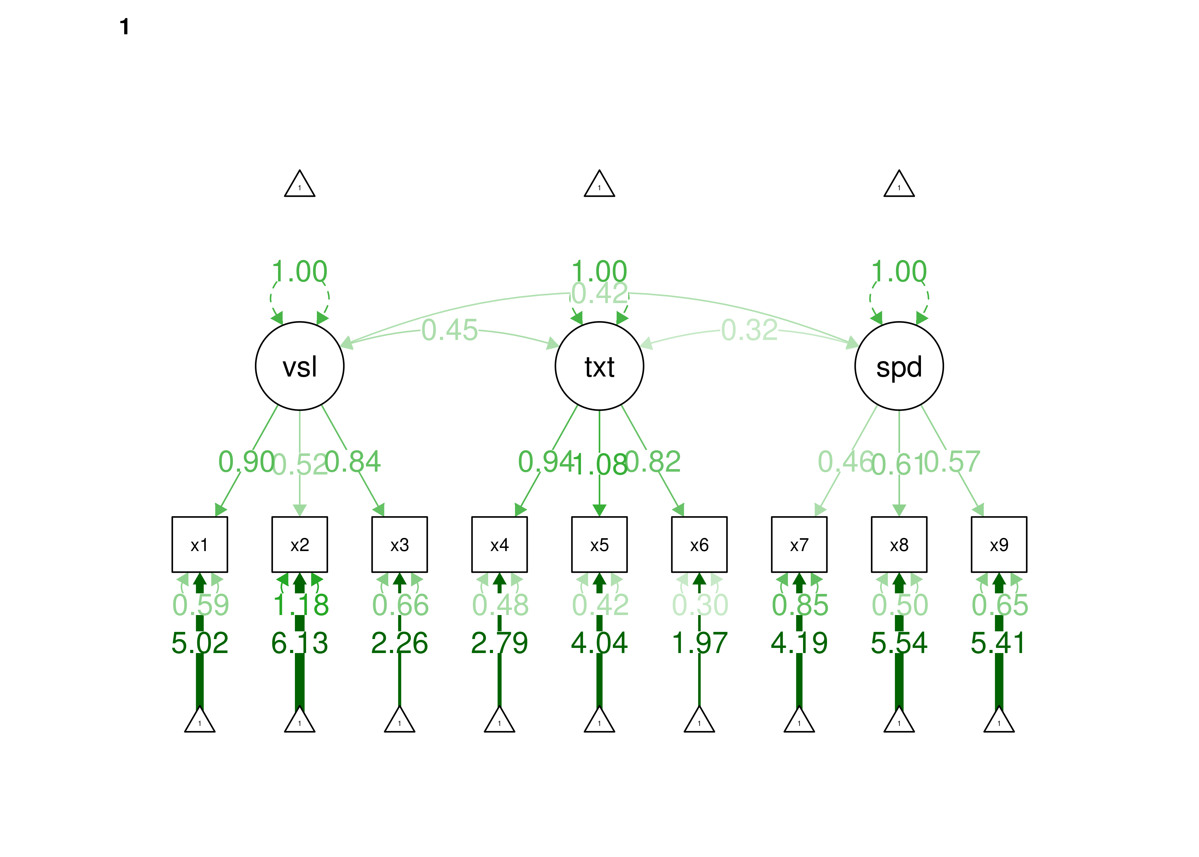
Figure 16.57: Scalar Invariance Model in Confirmatory Factor Analysis.
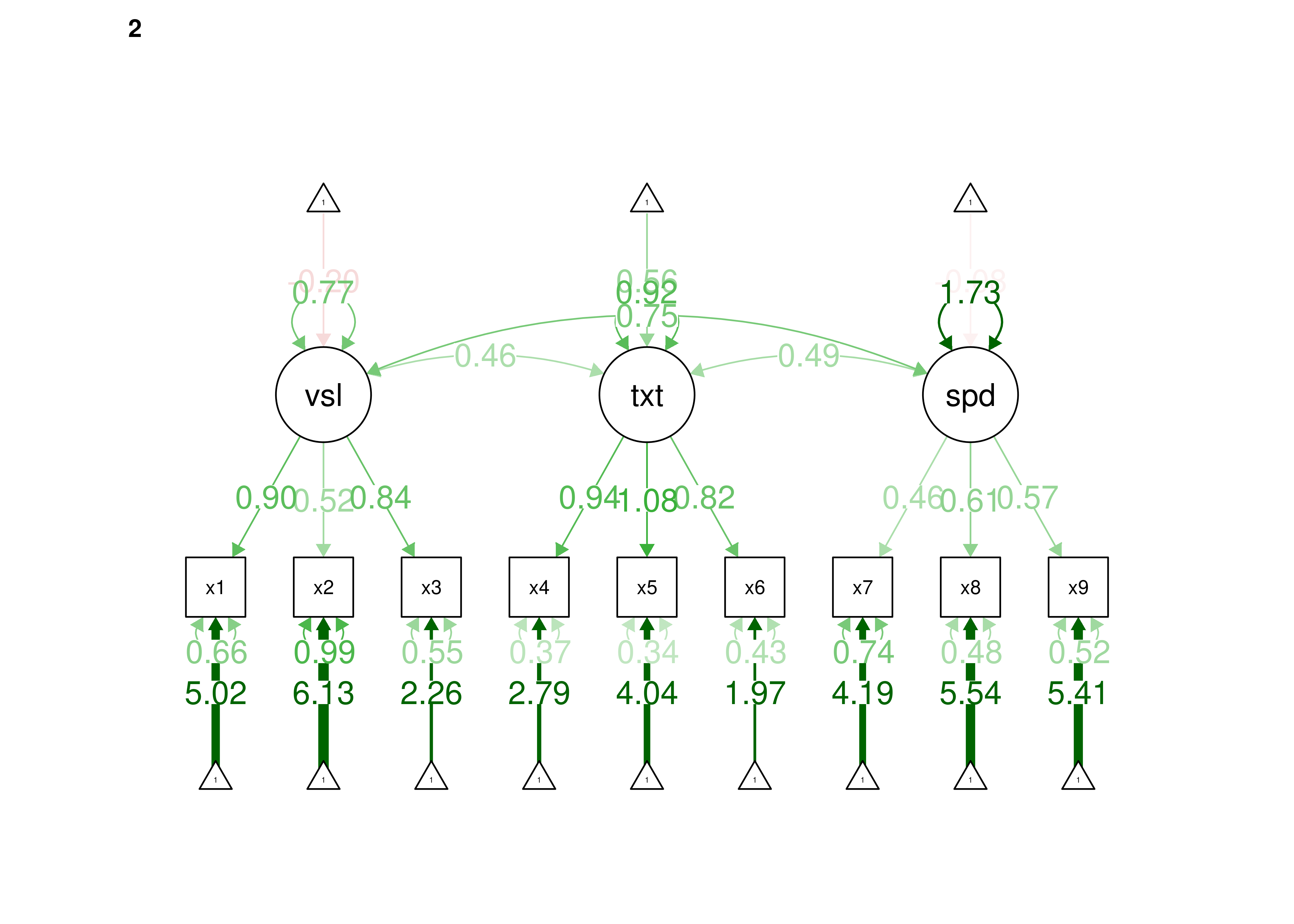
Figure 16.58: Scalar Invariance Model in Confirmatory Factor Analysis.
16.10.8 Residual (“Strict Factorial”) Invariance Model
Specify invariance of factor loadings, intercepts, and residuals across groups.
16.10.8.1 Model Syntax
Code
## LOADINGS:

visual =~ c(NA, NA)*x1 + c(lambda.1_1, lambda.1_1)*x1
visual =~ c(NA, NA)*x2 + c(lambda.2_1, lambda.2_1)*x2
visual =~ c(NA, NA)*x3 + c(lambda.3_1, lambda.3_1)*x3
textual =~ c(NA, NA)*x4 + c(lambda.4_2, lambda.4_2)*x4
textual =~ c(NA, NA)*x5 + c(lambda.5_2, lambda.5_2)*x5
textual =~ c(NA, NA)*x6 + c(lambda.6_2, lambda.6_2)*x6
speed =~ c(NA, NA)*x7 + c(lambda.7_3, lambda.7_3)*x7
speed =~ c(NA, NA)*x8 + c(lambda.8_3, lambda.8_3)*x8
speed =~ c(NA, NA)*x9 + c(lambda.9_3, lambda.9_3)*x9

## INTERCEPTS:

x1 ~ c(NA, NA)*1 + c(nu.1, nu.1)*1
x2 ~ c(NA, NA)*1 + c(nu.2, nu.2)*1
x3 ~ c(NA, NA)*1 + c(nu.3, nu.3)*1
x4 ~ c(NA, NA)*1 + c(nu.4, nu.4)*1
x5 ~ c(NA, NA)*1 + c(nu.5, nu.5)*1
x6 ~ c(NA, NA)*1 + c(nu.6, nu.6)*1
x7 ~ c(NA, NA)*1 + c(nu.7, nu.7)*1
x8 ~ c(NA, NA)*1 + c(nu.8, nu.8)*1
x9 ~ c(NA, NA)*1 + c(nu.9, nu.9)*1

## UNIQUE-FACTOR VARIANCES:

x1 ~~ c(NA, NA)*x1 + c(theta.1_1, theta.1_1)*x1
x2 ~~ c(NA, NA)*x2 + c(theta.2_2, theta.2_2)*x2
x3 ~~ c(NA, NA)*x3 + c(theta.3_3, theta.3_3)*x3
x4 ~~ c(NA, NA)*x4 + c(theta.4_4, theta.4_4)*x4
x5 ~~ c(NA, NA)*x5 + c(theta.5_5, theta.5_5)*x5
x6 ~~ c(NA, NA)*x6 + c(theta.6_6, theta.6_6)*x6
x7 ~~ c(NA, NA)*x7 + c(theta.7_7, theta.7_7)*x7
x8 ~~ c(NA, NA)*x8 + c(theta.8_8, theta.8_8)*x8
x9 ~~ c(NA, NA)*x9 + c(theta.9_9, theta.9_9)*x9

## LATENT MEANS/INTERCEPTS:

visual ~ c(0, NA)*1 + c(alpha.1.g1, alpha.1.g2)*1
textual ~ c(0, NA)*1 + c(alpha.2.g1, alpha.2.g2)*1
speed ~ c(0, NA)*1 + c(alpha.3.g1, alpha.3.g2)*1

## COMMON-FACTOR VARIANCES:

visual ~~ c(1, NA)*visual + c(psi.1_1.g1, psi.1_1.g2)*visual
textual ~~ c(1, NA)*textual + c(psi.2_2.g1, psi.2_2.g2)*textual
speed ~~ c(1, NA)*speed + c(psi.3_3.g1, psi.3_3.g2)*speed

## COMMON-FACTOR COVARIANCES:

visual ~~ c(NA, NA)*textual + c(psi.2_1.g1, psi.2_1.g2)*textual
visual ~~ c(NA, NA)*speed + c(psi.3_1.g1, psi.3_1.g2)*speed
textual ~~ c(NA, NA)*speed + c(psi.3_2.g1, psi.3_2.g2)*speed16.10.8.1.1 Summary of Model Features
This lavaan model syntax specifies a CFA with 9 manifest indicators of 3 common factor(s).

To identify the location and scale of each common factor, the factor means and variances were fixed to 0 and 1, respectively, unless equality constraints on measurement parameters allow them to be freed.

Pattern matrix indicating num(eric), ord(ered), and lat(ent) indicators per factor:

   visual textual speed
x1 num
x2 num
x3 num
x4        num
x5        num
x6        num
x7                num
x8                num
x9                num

The following types of parameter were constrained to equality across groups:

    loadings
    intercepts
residuals16.10.8.4 Model Summary
Code
lavaan 0.6-20 ended normally after 62 iterations

  Estimator                                         ML
  Optimization method                           NLMINB
  Number of model parameters                        66
  Number of equality constraints                    27

  Number of observations per group:
    Pasteur                                        156
    Grant-White                                    145
  Number of missing patterns per group:
    Pasteur                                          9
    Grant-White                                      9

Model Test User Model:
                                              Standard      Scaled
  Test Statistic                               172.960     172.714
  Degrees of freedom                                69          69
  P-value (Chi-square)                           0.000       0.000
  Scaling correction factor                                  1.001
    Yuan-Bentler correction (Mplus variant)
  Test statistic for each group:
    Pasteur                                     87.707      87.707
    Grant-White                                 85.007      85.007

Model Test Baseline Model:

  Test statistic                               932.665     909.019
  Degrees of freedom                                72          72
  P-value                                        0.000       0.000
  Scaling correction factor                                  1.026

User Model versus Baseline Model:

  Comparative Fit Index (CFI)                    0.879       0.876
  Tucker-Lewis Index (TLI)                       0.874       0.871

  Robust Comparative Fit Index (CFI)                         0.883
  Robust Tucker-Lewis Index (TLI)                            0.878

Loglikelihood and Information Criteria:

  Loglikelihood user model (H0)              -3680.600   -3680.600
  Scaling correction factor                                  0.645
      for the MLR correction
  Loglikelihood unrestricted model (H1)      -3594.120   -3594.120
  Scaling correction factor                                  1.034
      for the MLR correction

  Akaike (AIC)                                7439.201    7439.201
  Bayesian (BIC)                              7583.778    7583.778
  Sample-size adjusted Bayesian (SABIC)       7460.092    7460.092

Root Mean Square Error of Approximation:

  RMSEA                                          0.100       0.100
  90 Percent confidence interval - lower         0.082       0.081
  90 Percent confidence interval - upper         0.119       0.119
  P-value H_0: RMSEA <= 0.050                    0.000       0.000
  P-value H_0: RMSEA >= 0.080                    0.962       0.961

  Robust RMSEA                                               0.100
  90 Percent confidence interval - lower                     0.081
  90 Percent confidence interval - upper                     0.119
  P-value H_0: Robust RMSEA <= 0.050                         0.000
  P-value H_0: Robust RMSEA >= 0.080                         0.955

Standardized Root Mean Square Residual:

  SRMR                                           0.086       0.086

Parameter Estimates:

  Standard errors                             Sandwich
  Information bread                           Observed
  Observed information based on                Hessian


Group 1 [Pasteur]:

Latent Variables:
                   Estimate  Std.Err  z-value  P(>|z|)   Std.lv  Std.all
  visual =~
    x1      (l.1_)    0.862    0.126    6.855    0.000    0.862    0.728
    x2      (l.2_)    0.516    0.091    5.678    0.000    0.516    0.436
    x3      (l.3_)    0.745    0.112    6.630    0.000    0.745    0.651
  textual =~
    x4      (l.4_)    0.928    0.071   13.094    0.000    0.928    0.828
    x5      (l.5_)    1.069    0.076   14.113    0.000    1.069    0.855
    x6      (l.6_)    0.882    0.062   14.125    0.000    0.882    0.830
  speed =~
    x7      (l.7_)    0.577    0.087    6.658    0.000    0.577    0.544
    x8      (l.8_)    0.669    0.083    8.109    0.000    0.669    0.688
    x9      (l.9_)    0.632    0.085    7.461    0.000    0.632    0.649

Covariances:
                   Estimate  Std.Err  z-value  P(>|z|)   Std.lv  Std.all
  visual ~~
    textul  (p.2_)    0.430    0.124    3.472    0.001    0.430    0.430
    speed  (p.3_1)    0.351    0.129    2.710    0.007    0.351    0.351
  textual ~~
    speed  (p.3_2)    0.302    0.093    3.250    0.001    0.302    0.302

Intercepts:
                   Estimate  Std.Err  z-value  P(>|z|)   Std.lv  Std.all
   .x1      (nu.1)    5.025    0.095   52.938    0.000    5.025    4.243
   .x2      (nu.2)    6.138    0.086   71.711    0.000    6.138    5.188
   .x3      (nu.3)    2.332    0.099   23.546    0.000    2.332    2.039
   .x4      (nu.4)    2.784    0.086   32.453    0.000    2.784    2.483
   .x5      (nu.5)    4.030    0.102   39.369    0.000    4.030    3.224
   .x6      (nu.6)    1.928    0.075   25.828    0.000    1.928    1.815
   .x7      (nu.7)    4.270    0.076   55.911    0.000    4.270    4.027
   .x8      (nu.8)    5.619    0.075   74.597    0.000    5.619    5.775
   .x9      (nu.9)    5.470    0.073   74.756    0.000    5.470    5.616
    visual  (a.1.)    0.000                               0.000    0.000
    textual (a.2.)    0.000                               0.000    0.000
    speed   (a.3.)    0.000                               0.000    0.000

Variances:
                   Estimate  Std.Err  z-value  P(>|z|)   Std.lv  Std.all
   .x1      (t.1_)    0.660    0.165    4.008    0.000    0.660    0.470
   .x2      (t.2_)    1.133    0.110   10.337    0.000    1.133    0.810
   .x3      (t.3_)    0.754    0.131    5.749    0.000    0.754    0.576
   .x4      (t.4_)    0.396    0.050    7.904    0.000    0.396    0.315
   .x5      (t.5_)    0.420    0.057    7.385    0.000    0.420    0.269
   .x6      (t.6_)    0.350    0.048    7.311    0.000    0.350    0.310
   .x7      (t.7_)    0.792    0.094    8.413    0.000    0.792    0.704
   .x8      (t.8_)    0.499    0.095    5.244    0.000    0.499    0.527
   .x9      (t.9_)    0.549    0.100    5.479    0.000    0.549    0.579
    visual  (p.1_)    1.000                               1.000    1.000
    textual (p.2_)    1.000                               1.000    1.000
    speed   (p.3_)    1.000                               1.000    1.000

R-Square:
                   Estimate
    x1                0.530
    x2                0.190
    x3                0.424
    x4                0.685
    x5                0.731
    x6                0.690
    x7                0.296
    x8                0.473
    x9                0.421


Group 2 [Grant-White]:

Latent Variables:
                   Estimate  Std.Err  z-value  P(>|z|)   Std.lv  Std.all
  visual =~
    x1      (l.1_)    0.862    0.126    6.855    0.000    0.796    0.700
    x2      (l.2_)    0.516    0.091    5.678    0.000    0.476    0.408
    x3      (l.3_)    0.745    0.112    6.630    0.000    0.687    0.621
  textual =~
    x4      (l.4_)    0.928    0.071   13.094    0.000    0.926    0.827
    x5      (l.5_)    1.069    0.076   14.113    0.000    1.068    0.855
    x6      (l.6_)    0.882    0.062   14.125    0.000    0.881    0.830
  speed =~
    x7      (l.7_)    0.577    0.087    6.658    0.000    0.670    0.601
    x8      (l.8_)    0.669    0.083    8.109    0.000    0.777    0.740
    x9      (l.9_)    0.632    0.085    7.461    0.000    0.733    0.703

Covariances:
                   Estimate  Std.Err  z-value  P(>|z|)   Std.lv  Std.all
  visual ~~
    textul  (p.2_)    0.519    0.135    3.852    0.000    0.563    0.563
    speed  (p.3_1)    0.643    0.202    3.183    0.001    0.600    0.600
  textual ~~
    speed  (p.3_2)    0.426    0.181    2.351    0.019    0.368    0.368

Intercepts:
                   Estimate  Std.Err  z-value  P(>|z|)   Std.lv  Std.all
   .x1      (nu.1)    5.025    0.095   52.938    0.000    5.025    4.420
   .x2      (nu.2)    6.138    0.086   71.711    0.000    6.138    5.263
   .x3      (nu.3)    2.332    0.099   23.546    0.000    2.332    2.106
   .x4      (nu.4)    2.784    0.086   32.453    0.000    2.784    2.486
   .x5      (nu.5)    4.030    0.102   39.369    0.000    4.030    3.228
   .x6      (nu.6)    1.928    0.075   25.828    0.000    1.928    1.817
   .x7      (nu.7)    4.270    0.076   55.911    0.000    4.270    3.835
   .x8      (nu.8)    5.619    0.075   74.597    0.000    5.619    5.353
   .x9      (nu.9)    5.470    0.073   74.756    0.000    5.470    5.247
    visual  (a.1.)   -0.208    0.181   -1.149    0.251   -0.225   -0.225
    textual (a.2.)    0.611    0.132    4.646    0.000    0.612    0.612
    speed   (a.3.)   -0.283    0.155   -1.824    0.068   -0.244   -0.244

Variances:
                   Estimate  Std.Err  z-value  P(>|z|)   Std.lv  Std.all
   .x1      (t.1_)    0.660    0.165    4.008    0.000    0.660    0.510
   .x2      (t.2_)    1.133    0.110   10.337    0.000    1.133    0.833
   .x3      (t.3_)    0.754    0.131    5.749    0.000    0.754    0.615
   .x4      (t.4_)    0.396    0.050    7.904    0.000    0.396    0.316
   .x5      (t.5_)    0.420    0.057    7.385    0.000    0.420    0.269
   .x6      (t.6_)    0.350    0.048    7.311    0.000    0.350    0.311
   .x7      (t.7_)    0.792    0.094    8.413    0.000    0.792    0.638
   .x8      (t.8_)    0.499    0.095    5.244    0.000    0.499    0.453
   .x9      (t.9_)    0.549    0.100    5.479    0.000    0.549    0.505
    visual  (p.1_)    0.852    0.217    3.932    0.000    1.000    1.000
    textual (p.2_)    0.997    0.193    5.160    0.000    1.000    1.000
    speed   (p.3_)    1.346    0.328    4.101    0.000    1.000    1.000

R-Square:
                   Estimate
    x1                0.490
    x2                0.167
    x3                0.385
    x4                0.684
    x5                0.731
    x6                0.689
    x7                0.362
    x8                0.547
    x9                0.495
Code
lavaan 0.6-20 ended normally after 59 iterations

  Estimator                                         ML
  Optimization method                           NLMINB
  Number of model parameters                        66
  Number of equality constraints                    27

  Number of observations per group:
    Pasteur                                        156
    Grant-White                                    145
  Number of missing patterns per group:
    Pasteur                                          9
    Grant-White                                      9

Model Test User Model:
                                              Standard      Scaled
  Test Statistic                               172.960     172.714
  Degrees of freedom                                69          69
  P-value (Chi-square)                           0.000       0.000
  Scaling correction factor                                  1.001
    Yuan-Bentler correction (Mplus variant)
  Test statistic for each group:
    Pasteur                                     87.707      87.707
    Grant-White                                 85.007      85.007

Model Test Baseline Model:

  Test statistic                               932.665     909.019
  Degrees of freedom                                72          72
  P-value                                        0.000       0.000
  Scaling correction factor                                  1.026

User Model versus Baseline Model:

  Comparative Fit Index (CFI)                    0.879       0.876
  Tucker-Lewis Index (TLI)                       0.874       0.871

  Robust Comparative Fit Index (CFI)                         0.883
  Robust Tucker-Lewis Index (TLI)                            0.878

Loglikelihood and Information Criteria:

  Loglikelihood user model (H0)              -3680.600   -3680.600
  Scaling correction factor                                  0.645
      for the MLR correction
  Loglikelihood unrestricted model (H1)      -3594.120   -3594.120
  Scaling correction factor                                  1.034
      for the MLR correction

  Akaike (AIC)                                7439.201    7439.201
  Bayesian (BIC)                              7583.778    7583.778
  Sample-size adjusted Bayesian (SABIC)       7460.092    7460.092

Root Mean Square Error of Approximation:

  RMSEA                                          0.100       0.100
  90 Percent confidence interval - lower         0.082       0.081
  90 Percent confidence interval - upper         0.119       0.119
  P-value H_0: RMSEA <= 0.050                    0.000       0.000
  P-value H_0: RMSEA >= 0.080                    0.962       0.961

  Robust RMSEA                                               0.100
  90 Percent confidence interval - lower                     0.081
  90 Percent confidence interval - upper                     0.119
  P-value H_0: Robust RMSEA <= 0.050                         0.000
  P-value H_0: Robust RMSEA >= 0.080                         0.955

Standardized Root Mean Square Residual:

  SRMR                                           0.086       0.086

Parameter Estimates:

  Standard errors                             Sandwich
  Information bread                           Observed
  Observed information based on                Hessian


Group 1 [Pasteur]:

Latent Variables:
                   Estimate  Std.Err  z-value  P(>|z|)   Std.lv  Std.all
  visual =~
    x1      (lmb1)    0.862    0.126    6.855    0.000    0.862    0.728
    x2      (lmb2)    0.516    0.091    5.678    0.000    0.516    0.436
    x3      (lmb3)    0.745    0.112    6.630    0.000    0.745    0.651
  textual =~
    x4      (lmb4)    0.928    0.071   13.094    0.000    0.928    0.828
    x5      (lmb5)    1.069    0.076   14.113    0.000    1.069    0.855
    x6      (lmb6)    0.882    0.062   14.125    0.000    0.882    0.830
  speed =~
    x7      (lmb7)    0.577    0.087    6.658    0.000    0.577    0.544
    x8      (lmb8)    0.669    0.083    8.110    0.000    0.669    0.688
    x9      (lmb9)    0.632    0.085    7.461    0.000    0.632    0.649

Covariances:
                   Estimate  Std.Err  z-value  P(>|z|)   Std.lv  Std.all
  visual ~~
    textual           0.430    0.124    3.472    0.001    0.430    0.430
    speed             0.351    0.129    2.710    0.007    0.351    0.351
  textual ~~
    speed             0.302    0.093    3.250    0.001    0.302    0.302

Intercepts:
                   Estimate  Std.Err  z-value  P(>|z|)   Std.lv  Std.all
    visual            0.000                               0.000    0.000
    textual           0.000                               0.000    0.000
    speed             0.000                               0.000    0.000
   .x1      (int1)    5.025    0.095   52.938    0.000    5.025    4.243
   .x2      (int2)    6.138    0.086   71.710    0.000    6.138    5.188
   .x3      (int3)    2.332    0.099   23.546    0.000    2.332    2.039
   .x4      (int4)    2.784    0.086   32.453    0.000    2.784    2.483
   .x5      (int5)    4.030    0.102   39.369    0.000    4.030    3.224
   .x6      (int6)    1.928    0.075   25.828    0.000    1.928    1.815
   .x7      (int7)    4.270    0.076   55.911    0.000    4.270    4.027
   .x8      (int8)    5.619    0.075   74.598    0.000    5.619    5.775
   .x9      (int9)    5.470    0.073   74.756    0.000    5.470    5.616

Variances:
                   Estimate  Std.Err  z-value  P(>|z|)   Std.lv  Std.all
    visual            1.000                               1.000    1.000
    textual           1.000                               1.000    1.000
    speed             1.000                               1.000    1.000
   .x1      (rsd1)    0.660    0.165    4.008    0.000    0.660    0.470
   .x2      (rsd2)    1.133    0.110   10.337    0.000    1.133    0.810
   .x3      (rsd3)    0.754    0.131    5.749    0.000    0.754    0.576
   .x4      (rsd4)    0.396    0.050    7.904    0.000    0.396    0.315
   .x5      (rsd5)    0.420    0.057    7.385    0.000    0.420    0.269
   .x6      (rsd6)    0.350    0.048    7.311    0.000    0.350    0.310
   .x7      (rsd7)    0.792    0.094    8.414    0.000    0.792    0.704
   .x8      (rsd8)    0.499    0.095    5.244    0.000    0.499    0.527
   .x9      (rsd9)    0.549    0.100    5.479    0.000    0.549    0.579

R-Square:
                   Estimate
    x1                0.530
    x2                0.190
    x3                0.424
    x4                0.685
    x5                0.731
    x6                0.690
    x7                0.296
    x8                0.473
    x9                0.421


Group 2 [Grant-White]:

Latent Variables:
                   Estimate  Std.Err  z-value  P(>|z|)   Std.lv  Std.all
  visual =~
    x1      (lmb1)    0.862    0.126    6.855    0.000    0.796    0.700
    x2      (lmb2)    0.516    0.091    5.678    0.000    0.476    0.408
    x3      (lmb3)    0.745    0.112    6.630    0.000    0.687    0.621
  textual =~
    x4      (lmb4)    0.928    0.071   13.094    0.000    0.926    0.827
    x5      (lmb5)    1.069    0.076   14.113    0.000    1.068    0.855
    x6      (lmb6)    0.882    0.062   14.125    0.000    0.881    0.830
  speed =~
    x7      (lmb7)    0.577    0.087    6.658    0.000    0.670    0.601
    x8      (lmb8)    0.669    0.083    8.110    0.000    0.777    0.740
    x9      (lmb9)    0.632    0.085    7.461    0.000    0.733    0.703

Covariances:
                   Estimate  Std.Err  z-value  P(>|z|)   Std.lv  Std.all
  visual ~~
    textual           0.519    0.135    3.852    0.000    0.563    0.563
    speed             0.643    0.202    3.183    0.001    0.600    0.600
  textual ~~
    speed             0.426    0.181    2.351    0.019    0.368    0.368

Intercepts:
                   Estimate  Std.Err  z-value  P(>|z|)   Std.lv  Std.all
    visual           -0.208    0.181   -1.149    0.251   -0.225   -0.225
    textual           0.611    0.132    4.646    0.000    0.612    0.612
    speed            -0.283    0.155   -1.824    0.068   -0.244   -0.244
   .x1      (int1)    5.025    0.095   52.938    0.000    5.025    4.420
   .x2      (int2)    6.138    0.086   71.710    0.000    6.138    5.263
   .x3      (int3)    2.332    0.099   23.546    0.000    2.332    2.106
   .x4      (int4)    2.784    0.086   32.453    0.000    2.784    2.486
   .x5      (int5)    4.030    0.102   39.369    0.000    4.030    3.228
   .x6      (int6)    1.928    0.075   25.828    0.000    1.928    1.817
   .x7      (int7)    4.270    0.076   55.911    0.000    4.270    3.835
   .x8      (int8)    5.619    0.075   74.598    0.000    5.619    5.353
   .x9      (int9)    5.470    0.073   74.756    0.000    5.470    5.247

Variances:
                   Estimate  Std.Err  z-value  P(>|z|)   Std.lv  Std.all
    visual            0.852    0.217    3.932    0.000    1.000    1.000
    textual           0.997    0.193    5.160    0.000    1.000    1.000
    speed             1.346    0.328    4.101    0.000    1.000    1.000
   .x1      (rsd1)    0.660    0.165    4.008    0.000    0.660    0.510
   .x2      (rsd2)    1.133    0.110   10.337    0.000    1.133    0.833
   .x3      (rsd3)    0.754    0.131    5.749    0.000    0.754    0.615
   .x4      (rsd4)    0.396    0.050    7.904    0.000    0.396    0.316
   .x5      (rsd5)    0.420    0.057    7.385    0.000    0.420    0.269
   .x6      (rsd6)    0.350    0.048    7.311    0.000    0.350    0.311
   .x7      (rsd7)    0.792    0.094    8.414    0.000    0.792    0.638
   .x8      (rsd8)    0.499    0.095    5.244    0.000    0.499    0.453
   .x9      (rsd9)    0.549    0.100    5.479    0.000    0.549    0.505

R-Square:
                   Estimate
    x1                0.490
    x2                0.167
    x3                0.385
    x4                0.684
    x5                0.731
    x6                0.689
    x7                0.362
    x8                0.547
    x9                0.495
16.10.8.5 Model Fit
You can specify the null model as the baseline model using: baseline.model = nullModelFit
                         npar                          fmin
                       39.000                         0.287
                        chisq                            df
                      172.960                        69.000
                       pvalue                  chisq.scaled
                        0.000                       172.714
                    df.scaled                 pvalue.scaled
                       69.000                         0.000
         chisq.scaling.factor                baseline.chisq
                        1.001                       932.665
                  baseline.df               baseline.pvalue
                       72.000                         0.000
        baseline.chisq.scaled            baseline.df.scaled
                      909.019                        72.000
       baseline.pvalue.scaled baseline.chisq.scaling.factor
                        0.000                         1.026
                          cfi                           tli
                        0.879                         0.874
                   cfi.scaled                    tli.scaled
                        0.876                         0.871
                   cfi.robust                    tli.robust
                        0.883                         0.878
                         nnfi                           rfi
                        0.874                         0.806
                          nfi                          pnfi
                        0.815                         0.781
                          ifi                           rni
                        0.880                         0.879
                  nnfi.scaled                    rfi.scaled
                        0.871                         0.802
                   nfi.scaled                   pnfi.scaled
                        0.810                         0.776
                   ifi.scaled                    rni.scaled
                        0.877                         0.876
                  nnfi.robust                    rni.robust
                        0.878                         0.883
                         logl             unrestricted.logl
                    -3680.600                     -3594.120
                          aic                           bic
                     7439.201                      7583.778
                       ntotal                          bic2
                      301.000                      7460.092
            scaling.factor.h1             scaling.factor.h0
                        1.034                         0.645
                        rmsea                rmsea.ci.lower
                        0.100                         0.082
               rmsea.ci.upper                rmsea.ci.level
                        0.119                         0.900
                 rmsea.pvalue                rmsea.close.h0
                        0.000                         0.050
        rmsea.notclose.pvalue             rmsea.notclose.h0
                        0.962                         0.080
                 rmsea.scaled         rmsea.ci.lower.scaled
                        0.100                         0.081
        rmsea.ci.upper.scaled           rmsea.pvalue.scaled
                        0.119                         0.000
 rmsea.notclose.pvalue.scaled                  rmsea.robust
                        0.961                         0.100
        rmsea.ci.lower.robust         rmsea.ci.upper.robust
                        0.081                         0.119
          rmsea.pvalue.robust  rmsea.notclose.pvalue.robust
                        0.000                         0.955
                          rmr                    rmr_nomean
                        0.103                         0.102
                         srmr                  srmr_bentler
                        0.086                         0.086
          srmr_bentler_nomean                          crmr
                        0.083                         0.086
                  crmr_nomean                    srmr_mplus
                        0.083                         0.104
            srmr_mplus_nomean                         cn_05
                        0.084                       156.566
                        cn_01                           gfi
                      173.684                         0.992
                         agfi                          pgfi
                        0.988                         0.634
                          mfi                          ecvi
                        0.841                         0.834
Code
residualInvarianceModelFitIndices <- fitMeasures(
  residualInvarianceModel_fit)[c(
    "cfi.robust", "rmsea.robust", "srmr")]

residualInvarianceModel_chisquare <- fitMeasures(
  residualInvarianceModel_fit)[c("chisq.scaled")]

residualInvarianceModel_chisquareScaling <- fitMeasures(
  residualInvarianceModel_fit)[c("chisq.scaling.factor")]

residualInvarianceModel_df <- fitMeasures(
  residualInvarianceModel_fit)[c("df.scaled")]

residualInvarianceModel_N <- lavInspect(
  residualInvarianceModel_fit,
  what = "ntotal")
16.10.8.6 Compare Model Fit
16.10.8.6.1 Nested Model (\(\chi^2\)) Difference Test
The scalar invariance model and the residual invariance model are considered “nested” models. The residual invariance model is nested within the scalar invariance model because the scalar invariance model includes all of the terms of the residual invariance model along with additional terms. Model fit of nested models can be compared with a chi-square difference test, also known as a likelihood ratio test or deviance test. A significant chi-square difference test would indicate that the simplified model with additional constraints (the residual invariance model) is significantly worse fitting than the more complex model that has fewer constraints (the scalar invariance model).
In this instance, you do not need to examine whether residual invariance held because the preceding level of measurement invariance (scalar invariance) did not hold.
The petersenlab package (Petersen, 2025) contains the satorraBentlerScaledChiSquareDifferenceTestStatistic() function that performs a Satorra-Bentler scaled chi-square difference test:
Code
residualInvarianceModel_chisquareDiff <-
  satorraBentlerScaledChiSquareDifferenceTestStatistic(
    T0 = residualInvarianceModel_chisquare,
    c0 = residualInvarianceModel_chisquareScaling,
    d0 = residualInvarianceModel_df,
    T1 = scalarInvarianceModel_chisquare,
    c1 = scalarInvarianceModel_chisquareScaling,
    d1 = scalarInvarianceModel_df)

residualInvarianceModel_chisquareDiff
chisq.scaled
14.35586 16.10.8.6.3 Score-Based Test
Score-based tests of measurement invariance are implemented using the strucchange package and are described by T. Wang et al. (2014).
lambda.1_1 lambda.2_1 lambda.3_1 lambda.4_2 lambda.5_2 lambda.6_2 lambda.7_3
     0.862      0.516      0.745      0.928      1.069      0.882      0.577
lambda.8_3 lambda.9_3       nu.1       nu.2       nu.3       nu.4       nu.5
     0.669      0.632      5.025      6.138      2.332      2.784      4.030
      nu.6       nu.7       nu.8       nu.9  theta.1_1  theta.2_2  theta.3_3
     1.928      4.270      5.619      5.470      0.660      1.133      0.754
 theta.4_4  theta.5_5  theta.6_6  theta.7_7  theta.8_8  theta.9_9 psi.2_1.g1
     0.396      0.420      0.350      0.792      0.499      0.549      0.430
psi.3_1.g1 psi.3_2.g1 lambda.1_1 lambda.2_1 lambda.3_1 lambda.4_2 lambda.5_2
     0.351      0.302      0.862      0.516      0.745      0.928      1.069
lambda.6_2 lambda.7_3 lambda.8_3 lambda.9_3       nu.1       nu.2       nu.3
     0.882      0.577      0.669      0.632      5.025      6.138      2.332
      nu.4       nu.5       nu.6       nu.7       nu.8       nu.9  theta.1_1
     2.784      4.030      1.928      4.270      5.619      5.470      0.660
 theta.2_2  theta.3_3  theta.4_4  theta.5_5  theta.6_6  theta.7_7  theta.8_8
     1.133      0.754      0.396      0.420      0.350      0.792      0.499
 theta.9_9 alpha.1.g2 alpha.2.g2 alpha.3.g2 psi.1_1.g2 psi.2_2.g2 psi.3_3.g2
     0.549     -0.208      0.611     -0.283      0.852      0.997      1.346
psi.2_1.g2 psi.3_1.g2 psi.3_2.g2
0.519 0.643 0.426 theta.1_1 theta.2_2 theta.3_3 theta.4_4 theta.5_5 theta.6_6 theta.7_7 theta.8_8
0.6598353 1.1333770 0.7536794 0.3957809 0.4196626 0.3504637 0.7916721 0.4987961
theta.9_9
0.5490913 Code
    M-fluctuation test

data:  residualInvarianceModel_fit
f(efp) = 10.64, p-value = 0.3012
A score-based test and expected parameter change (EPC) estimates (Oberski, 2014; Oberski et al., 2015) are provided by the lavaan package (Rosseel et al., 2022).
$test

total score test:

   test     X2 df p.value
1 score 60.136 27       0

$uni

univariate score tests:

     lhs op   rhs     X2 df p.value
1   .p1. == .p37.  0.011  1   0.915
2   .p2. == .p38.  0.043  1   0.836
3   .p3. == .p39.  0.062  1   0.803
4   .p4. == .p40.  0.089  1   0.766
5   .p5. == .p41.  4.083  1   0.043
6   .p6. == .p42.  5.815  1   0.016
7   .p7. == .p43.  0.026  1   0.872
8   .p8. == .p44.  0.003  1   0.954
9   .p9. == .p45.  0.006  1   0.939
10 .p10. == .p46.  6.331  1   0.012
11 .p11. == .p47.  7.812  1   0.005
12 .p12. == .p48. 20.213  1   0.000
13 .p13. == .p49.  1.231  1   0.267
14 .p14. == .p50.  1.155  1   0.283
15 .p15. == .p51.  0.001  1   0.982
16 .p16. == .p52. 14.986  1   0.000
17 .p17. == .p53.  3.574  1   0.059
18 .p18. == .p54.  1.735  1   0.188
19 .p19. == .p55.  0.055  1   0.815
20 .p20. == .p56.  2.026  1   0.155
21 .p21. == .p57.  1.867  1   0.172
22 .p22. == .p58.  0.754  1   0.385
23 .p23. == .p59.  0.619  1   0.432
24 .p24. == .p60.  3.852  1   0.050
25 .p25. == .p61.  2.273  1   0.132
26 .p26. == .p62.  0.674  1   0.412
27 .p27. == .p63.  1.954  1   0.162

$epc

expected parameter changes (epc) and expected parameter values (epv):

       lhs op     rhs block group free      label plabel    est    epc    epv
1   visual =~      x1     1     1    1 lambda.1_1   .p1.  0.862  0.083  0.945
2   visual =~      x2     1     1    2 lambda.2_1   .p2.  0.516 -0.017  0.499
3   visual =~      x3     1     1    3 lambda.3_1   .p3.  0.745 -0.095  0.650
4  textual =~      x4     1     1    4 lambda.4_2   .p4.  0.928 -0.006  0.922
5  textual =~      x5     1     1    5 lambda.5_2   .p5.  1.069  0.060  1.130
6  textual =~      x6     1     1    6 lambda.6_2   .p6.  0.882 -0.054  0.828
7    speed =~      x7     1     1    7 lambda.7_3   .p7.  0.577 -0.036  0.541
8    speed =~      x8     1     1    8 lambda.8_3   .p8.  0.669  0.006  0.676
9    speed =~      x9     1     1    9 lambda.9_3   .p9.  0.632 -0.028  0.604
10      x1 ~1             1     1   10       nu.1  .p10.  5.025 -0.076  4.949
11      x2 ~1             1     1   11       nu.2  .p11.  6.138 -0.154  5.984
12      x3 ~1             1     1   12       nu.3  .p12.  2.332  0.177  2.509
13      x4 ~1             1     1   13       nu.4  .p13.  2.784  0.030  2.814
14      x5 ~1             1     1   14       nu.5  .p14.  4.030 -0.029  4.002
15      x6 ~1             1     1   15       nu.6  .p15.  1.928  0.001  1.929
16      x7 ~1             1     1   16       nu.7  .p16.  4.270  0.168  4.439
17      x8 ~1             1     1   17       nu.8  .p17.  5.619 -0.055  5.564
18      x9 ~1             1     1   18       nu.9  .p18.  5.470 -0.043  5.427
19      x1 ~~      x1     1     1   19  theta.1_1  .p19.  0.660 -0.145  0.514
20      x2 ~~      x2     1     1   20  theta.2_2  .p20.  1.133  0.145  1.279
21      x3 ~~      x3     1     1   21  theta.3_3  .p21.  0.754  0.194  0.947
22      x4 ~~      x4     1     1   22  theta.4_4  .p22.  0.396  0.046  0.442
23      x5 ~~      x5     1     1   23  theta.5_5  .p23.  0.420  0.009  0.428
24      x6 ~~      x6     1     1   24  theta.6_6  .p24.  0.350 -0.059  0.291
25      x7 ~~      x7     1     1   25  theta.7_7  .p25.  0.792  0.115  0.906
26      x8 ~~      x8     1     1   26  theta.8_8  .p26.  0.499  0.016  0.515
27      x9 ~~      x9     1     1   27  theta.9_9  .p27.  0.549  0.084  0.633
28  visual ~1             1     1    0 alpha.1.g1  .p28.  0.000     NA     NA
29 textual ~1             1     1    0 alpha.2.g1  .p29.  0.000     NA     NA
30   speed ~1             1     1    0 alpha.3.g1  .p30.  0.000     NA     NA
31  visual ~~  visual     1     1    0 psi.1_1.g1  .p31.  1.000     NA     NA
32 textual ~~ textual     1     1    0 psi.2_2.g1  .p32.  1.000     NA     NA
33   speed ~~   speed     1     1    0 psi.3_3.g1  .p33.  1.000     NA     NA
34  visual ~~ textual     1     1   28 psi.2_1.g1  .p34.  0.430 -0.002  0.428
35  visual ~~   speed     1     1   29 psi.3_1.g1  .p35.  0.351  0.007  0.358
36 textual ~~   speed     1     1   30 psi.3_2.g1  .p36.  0.302  0.007  0.309
37  visual =~      x1     2     2   31 lambda.1_1  .p37.  0.862  0.000  0.862
38  visual =~      x2     2     2   32 lambda.2_1  .p38.  0.516  0.063  0.579
39  visual =~      x3     2     2   33 lambda.3_1  .p39.  0.745 -0.024  0.721
40 textual =~      x4     2     2   34 lambda.4_2  .p40.  0.928  0.036  0.963
41 textual =~      x5     2     2   35 lambda.5_2  .p41.  1.069 -0.091  0.978
42 textual =~      x6     2     2   36 lambda.6_2  .p42.  0.882  0.061  0.944
43   speed =~      x7     2     2   37 lambda.7_3  .p43.  0.577 -0.035  0.542
44   speed =~      x8     2     2   38 lambda.8_3  .p44.  0.669  0.020  0.689
45   speed =~      x9     2     2   39 lambda.9_3  .p45.  0.632  0.033  0.665
46      x1 ~1             2     2   40       nu.1  .p46.  5.025  0.075  5.100
47      x2 ~1             2     2   41       nu.2  .p47.  6.138  0.176  6.314
48      x3 ~1             2     2   42       nu.3  .p48.  2.332 -0.197  2.135
49      x4 ~1             2     2   43       nu.4  .p49.  2.784 -0.057  2.726
50      x5 ~1             2     2   44       nu.5  .p50.  4.030  0.085  4.115
51      x6 ~1             2     2   45       nu.6  .p51.  1.928 -0.040  1.888
52      x7 ~1             2     2   46       nu.7  .p52.  4.270 -0.185  4.086
53      x8 ~1             2     2   47       nu.8  .p53.  5.619  0.074  5.694
54      x9 ~1             2     2   48       nu.9  .p54.  5.470  0.065  5.535
55      x1 ~~      x1     2     2   49  theta.1_1  .p55.  0.660  0.021  0.681
56      x2 ~~      x2     2     2   50  theta.2_2  .p56.  1.133 -0.162  0.971
57      x3 ~~      x3     2     2   51  theta.3_3  .p57.  0.754 -0.091  0.663
58      x4 ~~      x4     2     2   52  theta.4_4  .p58.  0.396 -0.064  0.332
59      x5 ~~      x5     2     2   53  theta.5_5  .p59.  0.420  0.009  0.428
60      x6 ~~      x6     2     2   54  theta.6_6  .p60.  0.350  0.062  0.412
61      x7 ~~      x7     2     2   55  theta.7_7  .p61.  0.792 -0.088  0.704
62      x8 ~~      x8     2     2   56  theta.8_8  .p62.  0.499 -0.044  0.455
63      x9 ~~      x9     2     2   57  theta.9_9  .p63.  0.549 -0.095  0.454
64  visual ~1             2     2   58 alpha.1.g2  .p64. -0.208  0.009 -0.200
65 textual ~1             2     2   59 alpha.2.g2  .p65.  0.611  0.002  0.614
66   speed ~1             2     2   60 alpha.3.g2  .p66. -0.283 -0.016 -0.298
67  visual ~~  visual     2     2   61 psi.1_1.g2  .p67.  0.852  0.016  0.868
68 textual ~~ textual     2     2   62 psi.2_2.g2  .p68.  0.997 -0.004  0.993
69   speed ~~   speed     2     2   63 psi.3_3.g2  .p69.  1.346  0.008  1.354
70  visual ~~ textual     2     2   64 psi.2_1.g2  .p70.  0.519 -0.002  0.517
71  visual ~~   speed     2     2   65 psi.3_1.g2  .p71.  0.643 -0.014  0.629
72 textual ~~   speed     2     2   66 psi.3_2.g2  .p72.  0.426 -0.009  0.417
   sepc.lv sepc.all sepc.nox
1    0.083    0.070    0.070
2   -0.017   -0.014   -0.014
3   -0.095   -0.083   -0.083
4   -0.006   -0.005   -0.005
5    0.060    0.048    0.048
6   -0.054   -0.051   -0.051
7   -0.036   -0.034   -0.034
8    0.006    0.006    0.006
9   -0.028   -0.029   -0.029
10  -0.076   -0.065   -0.065
11  -0.154   -0.130   -0.130
12   0.177    0.155    0.155
13   0.030    0.027    0.027
14  -0.029   -0.023   -0.023
15   0.001    0.001    0.001
16   0.168    0.159    0.159
17  -0.055   -0.057   -0.057
18  -0.043   -0.044   -0.044
19  -0.660   -0.470   -0.470
20   1.133    0.810    0.810
21   0.754    0.576    0.576
22   0.396    0.315    0.315
23   0.420    0.269    0.269
24  -0.350   -0.310   -0.310
25   0.792    0.704    0.704
26   0.499    0.527    0.527
27   0.549    0.579    0.579
28      NA       NA       NA
29      NA       NA       NA
30      NA       NA       NA
31      NA       NA       NA
32      NA       NA       NA
33      NA       NA       NA
34  -0.002   -0.002   -0.002
35   0.007    0.007    0.007
36   0.007    0.007    0.007
37   0.000    0.000    0.000
38   0.058    0.050    0.050
39  -0.022   -0.020   -0.020
40   0.036    0.032    0.032
41  -0.091   -0.073   -0.073
42   0.061    0.058    0.058
43  -0.041   -0.037   -0.037
44   0.023    0.022    0.022
45   0.038    0.037    0.037
46   0.075    0.066    0.066
47   0.176    0.151    0.151
48  -0.197   -0.178   -0.178
49  -0.057   -0.051   -0.051
50   0.085    0.068    0.068
51  -0.040   -0.038   -0.038
52  -0.185   -0.166   -0.166
53   0.074    0.071    0.071
54   0.065    0.063    0.063
55   0.660    0.510    0.510
56  -1.133   -0.833   -0.833
57  -0.754   -0.615   -0.615
58  -0.396   -0.316   -0.316
59   0.420    0.269    0.269
60   0.350    0.311    0.311
61  -0.792   -0.638   -0.638
62  -0.499   -0.453   -0.453
63  -0.549   -0.505   -0.505
64   0.009    0.009    0.009
65   0.002    0.002    0.002
66  -0.013   -0.013   -0.013
67   1.000    1.000    1.000
68  -1.000   -1.000   -1.000
69   1.000    1.000    1.000
70  -0.002   -0.002   -0.002
71  -0.013   -0.013   -0.013
72  -0.007   -0.007   -0.007
16.10.8.6.4 Effect Size of Non-Invariance
The effect size of measurement non-invariance, as described by Nye et al. (2019), was calculated using the dmacs package (Dueber, 2019).
$DMACS
         visual      textual        speed
x1 7.757508e-16           NA           NA
x2 7.455410e-16           NA           NA
x3 1.273068e-16           NA           NA
x4           NA 4.817253e-16           NA
x5           NA 0.000000e+00           NA
x6           NA 3.340834e-16           NA
x7           NA           NA 7.914977e-16
x8           NA           NA 8.160377e-16
x9           NA           NA 8.988589e-16

$ItemDeltaMean
          visual      textual        speed
x1  8.829229e-16           NA           NA
x2  8.625798e-16           NA           NA
x3 -4.452136e-17           NA           NA
x4            NA 4.616772e-16           NA
x5            NA 0.000000e+00           NA
x6            NA 2.559985e-16           NA
x7            NA           NA 8.276666e-16
x8            NA           NA 7.760855e-16
x9            NA           NA 8.838053e-16

$MeanDiff
      visual      textual        speed
1.700981e-15 7.176757e-16 2.487557e-15
The \(w\) and \(\Delta \text{M}_\text{C}\) indices of the effect size of measurement non-invariance, as described by Newsom (2015), were calculated using the measurementNoninvarianceEffectSize() function of the petersenlab package (Petersen, 2025).
Code
$Mc_unconstrained
[1] 0.8507891

$Mc_constrained
[1] 0.8409128

$Delta_Mc
[1] 0.0098763

$w
[1] 0.07686594
16.10.8.6.5 Equivalence Test
The petersenlab package (Petersen, 2025) contains the equiv_chi() function from Counsell et al. (2020) that performs an equivalence test: https://osf.io/cqu8v.
The chi-square equivalence test is non-significant, suggesting that the model fit is not acceptable.
The equivalence test of the chi-square difference test is non-significant, suggesting that the degree of worsening of model fit is not acceptable.
Code
Moreover, the equivalence test of the chi-square difference test is non-significant, suggesting that the degree of worsening of model fit is not acceptable. In other words, residual invariance failed.
Code
16.10.8.6.6 Permutation Test
Permutation procedures for testing measurement invariance are described in (Jorgensen et al., 2018).
For reproducibility, I set the seed below.
Using the same seed will yield the same answer every time.
There is nothing special about this particular seed.
You can specify the null model as the baseline model using: baseline.model = nullModelFit.
Warning: this code takes a while to run based on \(100\) iterations. You can reduce the number of iterations to be faster.
Code
set.seed(52242)
residualInvarianceTest <- permuteMeasEq(
  nPermute = numPermutations,
  modelType = "mgcfa",
  con = residualInvarianceModel_fit,
  uncon = scalarInvarianceModel_fit,
  AFIs = myAFIs,
  moreAFIs = moreAFIs,
  parallelType = "multicore", #only 'snow' works on Windows, but right now, it is throwing an error
iseed = 52242)Omnibus p value based on parametric chi-squared difference test:
Chisq diff Df diff Pr(>Chisq)
14.356 9.000 0.110
Omnibus p values based on nonparametric permutation method:
AFI.Difference p.value
chisq 16.006 0.15
chisq.scaled 13.272 0.24
rmsea -0.004 0.38
cfi -0.008 0.15
tli 0.009 0.52
srmr 0.006 0.20
rmsea.robust -0.004 0.38
cfi.robust -0.007 0.15
tli.robust 0.010 0.50The p-values are non-significant, indicating that the model did not fit significantly worse than the scalar invariance model.
16.10.8.7 Internal Consistency Reliability
Internal consistency reliability of items composing the latent factors, as quantified by omega (\(\omega\)) and average variance extracted (AVE), was estimated using the semTools package (Jorgensen et al., 2021).
16.10.8.8 Path Diagram
A path diagram of the model generated using the semPlot package (Epskamp, 2022) is below.
Code
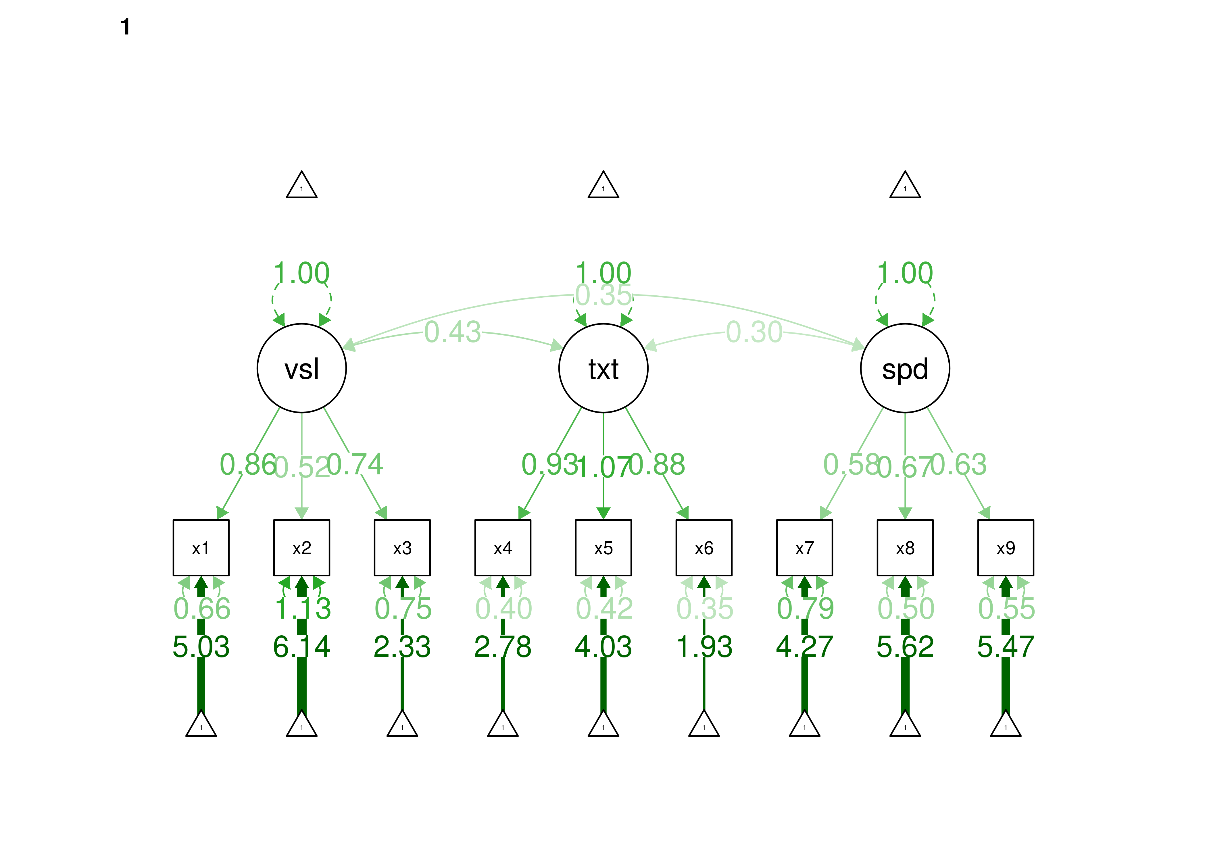
Figure 16.59: Residual Invariance Model in Confirmatory Factor Analysis.
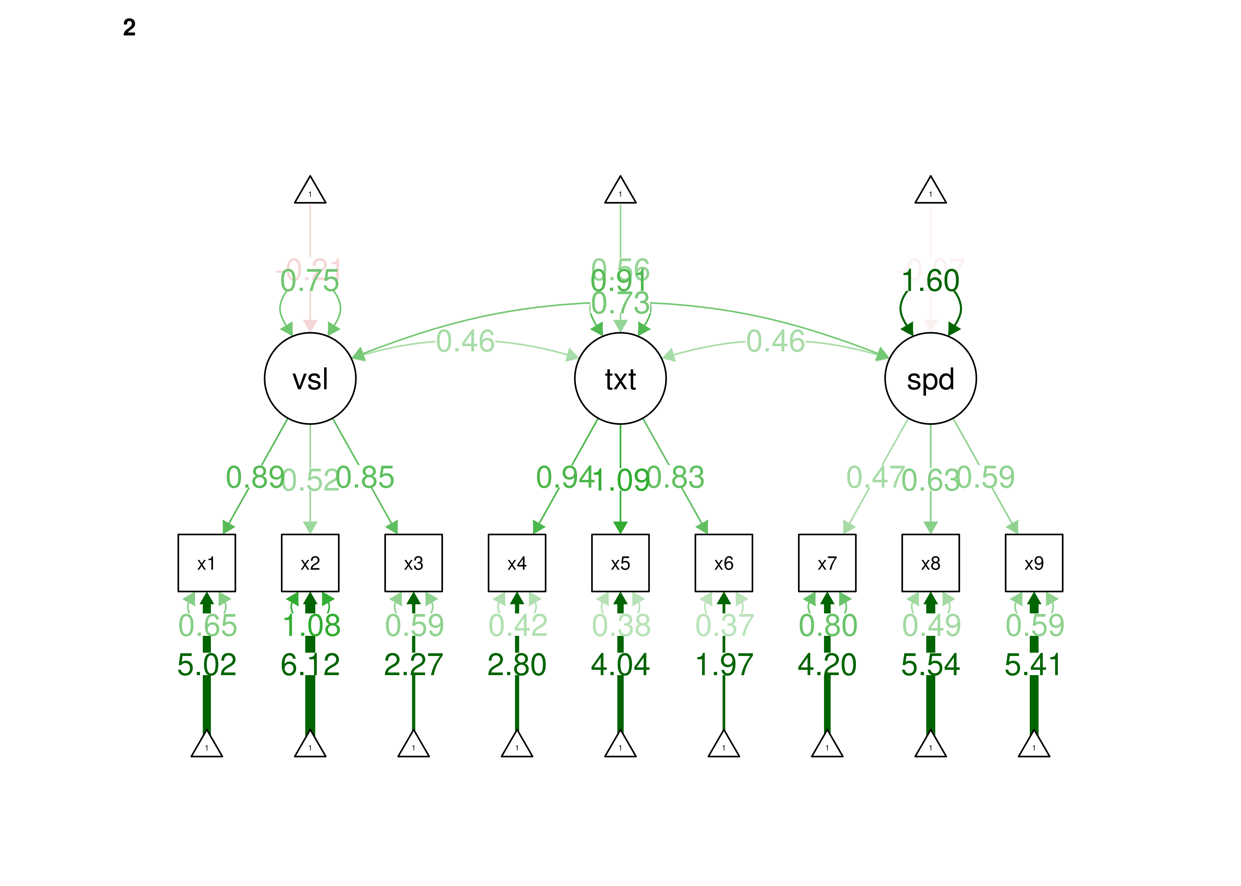
Figure 16.60: Residual Invariance Model in Confirmatory Factor Analysis.
16.10.9 Addressing Measurement Non-Invariance
In the example above, we detected measurement non-invariance of intercepts, but not factor loadings. Thus, we would want to identify which item(s) show non-invariant intercepts across groups. When detecting measurement non-invariance in a given parameter (e.g., factor loadings, intercepts, or residuals), one can identify the specific items that show measurement non-invariance in one of two primary ways: (1) starting with a model that allows the given parameter to differ across groups, a researcher can iteratively add constraints to identify the item(s) for which measurement invariance fails, or (2) starting with a model that constrains the given parameter to be the same across groups, a researcher can iteratively remove constraints to identify the item(s) for which measurement invariance becomes established (and by process of elimination, the items for which measurement invariance does not become established).
16.10.9.1 Iteratively add constraints to identify measurement non-invariance
In the example above, we detected measurement non-invariance of intercepts. One approach to identify measurement non-invariance is to iteratively add constraints to a model that allows the given parameter (intercepts) to differ across groups. So, we will use the metric invariance model as the baseline model (in which item intercepts are allowed to differ across groups), and iteratively add constraints to identify which item(s) show non-invariant intercepts across groups.
16.10.9.1.1 Variable 1
Variable 1 does not have non-invariant intercepts.
Code
cfaModel_metricInvarianceV1 <- '
 #Fix factor loadings to be the same across groups
 visual  =~ c(lambdax1,lambdax1)*x1 + c(lambdax2,lambdax2)*x2 + c(lambdax3,lambdax3)*x3
 textual =~ c(lambdax4,lambdax4)*x4 + c(lambdax5,lambdax5)*x5 + c(lambdax6,lambdax6)*x6
 speed   =~ c(lambdax7,lambdax7)*x7 + c(lambdax8,lambdax8)*x8 + c(lambdax9,lambdax9)*x9

 #Fix latent means to zero
 visual ~ 0
 textual ~ 0
 speed ~ 0

 #Fix latent variances to one in group 1; free latent variances in group 2
 visual ~~ c(1, NA)*visual
 textual ~~ c(1, NA)*textual
 speed ~~ c(1, NA)*speed

 #Estimate covariances among latent variables
 visual ~~ textual
 visual ~~ speed
 textual ~~ speed

 #Estimate residual variances of manifest variables
 x1 ~~ x1
 x2 ~~ x2
 x3 ~~ x3
 x4 ~~ x4
 x5 ~~ x5
 x6 ~~ x6
 x7 ~~ x7
 x8 ~~ x8
 x9 ~~ x9

 #Iteratively fix intercepts of manifest variables across groups
 x1 ~ c(intx1, intx1)*1
 x2 ~ NA*1
 x3 ~ NA*1
 x4 ~ NA*1
 x5 ~ NA*1
 x6 ~ NA*1
 x7 ~ NA*1
 x8 ~ NA*1
 x9 ~ NA*1
'

cfaModel_metricInvarianceV1_fit <- lavaan(
  cfaModel_metricInvarianceV1,
  data = HolzingerSwineford1939,
  group = "school",
  missing = "ML",
  estimator = "MLR")

anova(metricInvarianceModel_fit, cfaModel_metricInvarianceV1_fit)
16.10.9.1.2 Variable 2
Variable 2 has non-invariant intercepts.
Code
cfaModel_metricInvarianceV2 <- '
 #Fix factor loadings to be the same across groups
 visual  =~ c(lambdax1,lambdax1)*x1 + c(lambdax2,lambdax2)*x2 + c(lambdax3,lambdax3)*x3
 textual =~ c(lambdax4,lambdax4)*x4 + c(lambdax5,lambdax5)*x5 + c(lambdax6,lambdax6)*x6
 speed   =~ c(lambdax7,lambdax7)*x7 + c(lambdax8,lambdax8)*x8 + c(lambdax9,lambdax9)*x9

 #Fix latent means to zero
 visual ~ 0
 textual ~ 0
 speed ~ 0

 #Fix latent variances to one in group 1; free latent variances in group 2
 visual ~~ c(1, NA)*visual
 textual ~~ c(1, NA)*textual
 speed ~~ c(1, NA)*speed

 #Estimate covariances among latent variables
 visual ~~ textual
 visual ~~ speed
 textual ~~ speed

 #Estimate residual variances of manifest variables
 x1 ~~ x1
 x2 ~~ x2
 x3 ~~ x3
 x4 ~~ x4
 x5 ~~ x5
 x6 ~~ x6
 x7 ~~ x7
 x8 ~~ x8
 x9 ~~ x9

 #Iteratively fix intercepts of manifest variables across groups
 x1 ~ c(intx1, intx1)*1
 x2 ~ c(intx1, intx1)*1
 x3 ~ NA*1
 x4 ~ NA*1
 x5 ~ NA*1
 x6 ~ NA*1
 x7 ~ NA*1
 x8 ~ NA*1
 x9 ~ NA*1
'

cfaModel_metricInvarianceV2_fit <- lavaan(
  cfaModel_metricInvarianceV2,
  data = HolzingerSwineford1939,
  group = "school",
  missing = "ML",
  estimator = "MLR")

anova(metricInvarianceModel_fit, cfaModel_metricInvarianceV2_fit)
Variable 2 appears to have larger intercepts in group 2 than in group 1:
lavaan 0.6-20 ended normally after 73 iterations

  Estimator                                         ML
  Optimization method                           NLMINB
  Number of model parameters                        63
  Number of equality constraints                     9

  Number of observations per group:
    Pasteur                                        156
    Grant-White                                    145
  Number of missing patterns per group:
    Pasteur                                          9
    Grant-White                                      9

Model Test User Model:
                                              Standard      Scaled
  Test Statistic                               116.313     117.955
  Degrees of freedom                                54          54
  P-value (Chi-square)                           0.000       0.000
  Scaling correction factor                                  0.986
    Yuan-Bentler correction (Mplus variant)
  Test statistic for each group:
    Pasteur                                     64.366      64.366
    Grant-White                                 53.590      53.590

Parameter Estimates:

  Standard errors                             Sandwich
  Information bread                           Observed
  Observed information based on                Hessian


Group 1 [Pasteur]:

Latent Variables:
                   Estimate  Std.Err  z-value  P(>|z|)
  visual =~
    x1      (l.1_)    0.885    0.122    7.258    0.000
    x2      (l.2_)    0.536    0.088    6.106    0.000
    x3      (l.3_)    0.707    0.087    8.148    0.000
  textual =~
    x4      (l.4_)    0.935    0.072   12.929    0.000
    x5      (l.5_)    1.045    0.076   13.740    0.000
    x6      (l.6_)    0.874    0.070   12.496    0.000
  speed =~
    x7      (l.7_)    0.550    0.075    7.346    0.000
    x8      (l.8_)    0.675    0.087    7.784    0.000
    x9      (l.9_)    0.602    0.088    6.867    0.000

Covariances:
                   Estimate  Std.Err  z-value  P(>|z|)
  visual ~~
    textul  (p.2_)    0.473    0.105    4.484    0.000
    speed  (p.3_1)    0.347    0.125    2.778    0.005
  textual ~~
    speed  (p.3_2)    0.320    0.096    3.342    0.001

Intercepts:
                   Estimate  Std.Err  z-value  P(>|z|)
   .x1      (n.1.)    4.948    0.095   52.314    0.000
   .x2      (n.2.)    5.984    0.098   60.949    0.000
   .x3      (n.3.)    2.510    0.093   26.891    0.000
   .x4      (n.4.)    2.814    0.091   30.886    0.000
   .x5      (n.5.)    4.002    0.105   38.265    0.000
   .x6      (n.6.)    1.929    0.079   24.377    0.000
   .x7      (n.7.)    4.439    0.087   51.128    0.000
   .x8      (n.8.)    5.564    0.079   70.170    0.000
   .x9      (n.9.)    5.426    0.080   67.539    0.000
    visual  (a.1.)    0.000
    textual (a.2.)    0.000
    speed   (a.3.)    0.000

Variances:
                   Estimate  Std.Err  z-value  P(>|z|)
   .x1      (t.1_)    0.577    0.166    3.482    0.000
   .x2      (t.2_)    1.252    0.162    7.718    0.000
   .x3      (t.3_)    0.853    0.127    6.737    0.000
   .x4      (t.4_)    0.447    0.072    6.189    0.000
   .x5      (t.5_)    0.486    0.075    6.445    0.000
   .x6      (t.6_)    0.258    0.057    4.499    0.000
   .x7      (t.7_)    0.860    0.114    7.549    0.000
   .x8      (t.8_)    0.512    0.097    5.296    0.000
   .x9      (t.9_)    0.635    0.118    5.376    0.000
    visual  (p.1_)    1.000
    textual (p.2_)    1.000
    speed   (p.3_)    1.000


Group 2 [Grant-White]:

Latent Variables:
                   Estimate  Std.Err  z-value  P(>|z|)
  visual =~
    x1      (l.1_)    0.885    0.122    7.258    0.000
    x2      (l.2_)    0.536    0.088    6.106    0.000
    x3      (l.3_)    0.707    0.087    8.148    0.000
  textual =~
    x4      (l.4_)    0.935    0.072   12.929    0.000
    x5      (l.5_)    1.045    0.076   13.740    0.000
    x6      (l.6_)    0.874    0.070   12.496    0.000
  speed =~
    x7      (l.7_)    0.550    0.075    7.346    0.000
    x8      (l.8_)    0.675    0.087    7.784    0.000
    x9      (l.9_)    0.602    0.088    6.867    0.000

Covariances:
                   Estimate  Std.Err  z-value  P(>|z|)
  visual ~~
    textul  (p.2_)    0.520    0.134    3.867    0.000
    speed  (p.3_1)    0.638    0.211    3.023    0.002
  textual ~~
    speed  (p.3_2)    0.429    0.193    2.219    0.026

Intercepts:
                   Estimate  Std.Err  z-value  P(>|z|)
   .x1      (n.1.)    4.930    0.096   51.453    0.000
   .x2      (n.2.)    6.198    0.092   67.063    0.000
   .x3      (n.3.)    1.992    0.086   23.042    0.000
   .x4      (n.4.)    3.318    0.093   35.501    0.000
   .x5      (n.5.)    4.714    0.097   48.693    0.000
   .x6      (n.6.)    2.467    0.094   26.165    0.000
   .x7      (n.7.)    3.923    0.087   45.299    0.000
   .x8      (n.8.)    5.488    0.087   63.174    0.000
   .x9      (n.9.)    5.338    0.085   62.628    0.000
    visual  (a.1.)    0.000
    textual (a.2.)    0.000
    speed   (a.3.)    0.000

Variances:
                   Estimate  Std.Err  z-value  P(>|z|)
   .x1      (t.1_)    0.652    0.168    3.877    0.000
   .x2      (t.2_)    0.940    0.145    6.473    0.000
   .x3      (t.3_)    0.606    0.113    5.376    0.000
   .x4      (t.4_)    0.348    0.066    5.257    0.000
   .x5      (t.5_)    0.371    0.074    5.021    0.000
   .x6      (t.6_)    0.439    0.076    5.738    0.000
   .x7      (t.7_)    0.622    0.098    6.338    0.000
   .x8      (t.8_)    0.410    0.148    2.765    0.006
   .x9      (t.9_)    0.505    0.128    3.957    0.000
    visual  (p.1_)    0.910    0.234    3.895    0.000
    textual (p.2_)    1.004    0.191    5.257    0.000
    speed   (p.3_)    1.498    0.357    4.201    0.000
Thus, in subsequent models, we would allow variable 2 to have different intercepts across groups.
16.10.9.1.3 Variable 3
Variable 3 has non-invariant intercepts.
Code
cfaModel_metricInvarianceV3 <- '
 #Fix factor loadings to be the same across groups
 visual  =~ c(lambdax1,lambdax1)*x1 + c(lambdax2,lambdax2)*x2 + c(lambdax3,lambdax3)*x3
 textual =~ c(lambdax4,lambdax4)*x4 + c(lambdax5,lambdax5)*x5 + c(lambdax6,lambdax6)*x6
 speed   =~ c(lambdax7,lambdax7)*x7 + c(lambdax8,lambdax8)*x8 + c(lambdax9,lambdax9)*x9

 #Fix latent means to zero
 visual ~ 0
 textual ~ 0
 speed ~ 0

 #Fix latent variances to one in group 1; free latent variances in group 2
 visual ~~ c(1, NA)*visual
 textual ~~ c(1, NA)*textual
 speed ~~ c(1, NA)*speed

 #Estimate covariances among latent variables
 visual ~~ textual
 visual ~~ speed
 textual ~~ speed

 #Estimate residual variances of manifest variables
 x1 ~~ x1
 x2 ~~ x2
 x3 ~~ x3
 x4 ~~ x4
 x5 ~~ x5
 x6 ~~ x6
 x7 ~~ x7
 x8 ~~ x8
 x9 ~~ x9

 #Iteratively fix intercepts of manifest variables across groups
 x1 ~ c(intx1, intx1)*1
 x2 ~ NA*1
 x3 ~ c(intx1, intx1)*1
 x4 ~ NA*1
 x5 ~ NA*1
 x6 ~ NA*1
 x7 ~ NA*1
 x8 ~ NA*1
 x9 ~ NA*1
'

cfaModel_metricInvarianceV3_fit <- lavaan(
  cfaModel_metricInvarianceV3,
  data = HolzingerSwineford1939,
  group = "school",
  missing = "ML",
  estimator = "MLR")

anova(metricInvarianceModel_fit, cfaModel_metricInvarianceV3_fit)
16.10.9.1.4 Variable 4
Variable 4 has non-invariant intercepts.
Code
cfaModel_metricInvarianceV4 <- '
 #Fix factor loadings to be the same across groups
 visual  =~ c(lambdax1,lambdax1)*x1 + c(lambdax2,lambdax2)*x2 + c(lambdax3,lambdax3)*x3
 textual =~ c(lambdax4,lambdax4)*x4 + c(lambdax5,lambdax5)*x5 + c(lambdax6,lambdax6)*x6
 speed   =~ c(lambdax7,lambdax7)*x7 + c(lambdax8,lambdax8)*x8 + c(lambdax9,lambdax9)*x9

 #Fix latent means to zero
 visual ~ 0
 textual ~ 0
 speed ~ 0

 #Fix latent variances to one in group 1; free latent variances in group 2
 visual ~~ c(1, NA)*visual
 textual ~~ c(1, NA)*textual
 speed ~~ c(1, NA)*speed

 #Estimate covariances among latent variables
 visual ~~ textual
 visual ~~ speed
 textual ~~ speed

 #Estimate residual variances of manifest variables
 x1 ~~ x1
 x2 ~~ x2
 x3 ~~ x3
 x4 ~~ x4
 x5 ~~ x5
 x6 ~~ x6
 x7 ~~ x7
 x8 ~~ x8
 x9 ~~ x9

 #Iteratively fix intercepts of manifest variables across groups
 x1 ~ c(intx1, intx1)*1
 x2 ~ NA*1
 x3 ~ NA*1
 x4 ~ c(intx1, intx1)*1
 x5 ~ NA*1
 x6 ~ NA*1
 x7 ~ NA*1
 x8 ~ NA*1
 x9 ~ NA*1
'

cfaModel_metricInvarianceV4_fit <- lavaan(
  cfaModel_metricInvarianceV4,
  data = HolzingerSwineford1939,
  group = "school",
  missing = "ML",
  estimator = "MLR")

anova(metricInvarianceModel_fit, cfaModel_metricInvarianceV4_fit)
16.10.9.1.5 Variable 5
Variable 5 has non-invariant intercepts.
Code
cfaModel_metricInvarianceV5 <- '
 #Fix factor loadings to be the same across groups
 visual  =~ c(lambdax1,lambdax1)*x1 + c(lambdax2,lambdax2)*x2 + c(lambdax3,lambdax3)*x3
 textual =~ c(lambdax4,lambdax4)*x4 + c(lambdax5,lambdax5)*x5 + c(lambdax6,lambdax6)*x6
 speed   =~ c(lambdax7,lambdax7)*x7 + c(lambdax8,lambdax8)*x8 + c(lambdax9,lambdax9)*x9

 #Fix latent means to zero
 visual ~ 0
 textual ~ 0
 speed ~ 0

 #Fix latent variances to one in group 1; free latent variances in group 2
 visual ~~ c(1, NA)*visual
 textual ~~ c(1, NA)*textual
 speed ~~ c(1, NA)*speed

 #Estimate covariances among latent variables
 visual ~~ textual
 visual ~~ speed
 textual ~~ speed

 #Estimate residual variances of manifest variables
 x1 ~~ x1
 x2 ~~ x2
 x3 ~~ x3
 x4 ~~ x4
 x5 ~~ x5
 x6 ~~ x6
 x7 ~~ x7
 x8 ~~ x8
 x9 ~~ x9

 #Iteratively fix intercepts of manifest variables across groups
 x1 ~ c(intx1, intx1)*1
 x2 ~ NA*1
 x3 ~ NA*1
 x4 ~ NA*1
 x5 ~ c(intx1, intx1)*1
 x6 ~ NA*1
 x7 ~ NA*1
 x8 ~ NA*1
 x9 ~ NA*1
'

cfaModel_metricInvarianceV5_fit <- lavaan(
  cfaModel_metricInvarianceV5,
  data = HolzingerSwineford1939,
  group = "school",
  missing = "ML",
  estimator = "MLR")

anova(metricInvarianceModel_fit, cfaModel_metricInvarianceV5_fit)
16.10.9.1.6 Variable 6
Variable 6 has non-invariant intercepts.
Code
cfaModel_metricInvarianceV6 <- '
 #Fix factor loadings to be the same across groups
 visual  =~ c(lambdax1,lambdax1)*x1 + c(lambdax2,lambdax2)*x2 + c(lambdax3,lambdax3)*x3
 textual =~ c(lambdax4,lambdax4)*x4 + c(lambdax5,lambdax5)*x5 + c(lambdax6,lambdax6)*x6
 speed   =~ c(lambdax7,lambdax7)*x7 + c(lambdax8,lambdax8)*x8 + c(lambdax9,lambdax9)*x9

 #Fix latent means to zero
 visual ~ 0
 textual ~ 0
 speed ~ 0

 #Fix latent variances to one in group 1; free latent variances in group 2
 visual ~~ c(1, NA)*visual
 textual ~~ c(1, NA)*textual
 speed ~~ c(1, NA)*speed

 #Estimate covariances among latent variables
 visual ~~ textual
 visual ~~ speed
 textual ~~ speed

 #Estimate residual variances of manifest variables
 x1 ~~ x1
 x2 ~~ x2
 x3 ~~ x3
 x4 ~~ x4
 x5 ~~ x5
 x6 ~~ x6
 x7 ~~ x7
 x8 ~~ x8
 x9 ~~ x9

 #Iteratively fix intercepts of manifest variables across groups
 x1 ~ c(intx1, intx1)*1
 x2 ~ NA*1
 x3 ~ NA*1
 x4 ~ NA*1
 x5 ~ NA*1
 x6 ~ c(intx1, intx1)*1
 x7 ~ NA*1
 x8 ~ NA*1
 x9 ~ NA*1
'

cfaModel_metricInvarianceV6_fit <- lavaan(
  cfaModel_metricInvarianceV6,
  data = HolzingerSwineford1939,
  group = "school",
  missing = "ML",
  estimator = "MLR")

anova(metricInvarianceModel_fit, cfaModel_metricInvarianceV6_fit)
16.10.9.1.7 Variable 7
Variable 7 has non-invariant intercepts.
Code
cfaModel_metricInvarianceV7 <- '
 #Fix factor loadings to be the same across groups
 visual  =~ c(lambdax1,lambdax1)*x1 + c(lambdax2,lambdax2)*x2 + c(lambdax3,lambdax3)*x3
 textual =~ c(lambdax4,lambdax4)*x4 + c(lambdax5,lambdax5)*x5 + c(lambdax6,lambdax6)*x6
 speed   =~ c(lambdax7,lambdax7)*x7 + c(lambdax8,lambdax8)*x8 + c(lambdax9,lambdax9)*x9

 #Fix latent means to zero
 visual ~ 0
 textual ~ 0
 speed ~ 0

 #Fix latent variances to one in group 1; free latent variances in group 2
 visual ~~ c(1, NA)*visual
 textual ~~ c(1, NA)*textual
 speed ~~ c(1, NA)*speed

 #Estimate covariances among latent variables
 visual ~~ textual
 visual ~~ speed
 textual ~~ speed

 #Estimate residual variances of manifest variables
 x1 ~~ x1
 x2 ~~ x2
 x3 ~~ x3
 x4 ~~ x4
 x5 ~~ x5
 x6 ~~ x6
 x7 ~~ x7
 x8 ~~ x8
 x9 ~~ x9

 #Iteratively fix intercepts of manifest variables across groups
 x1 ~ c(intx1, intx1)*1
 x2 ~ NA*1
 x3 ~ NA*1
 x4 ~ NA*1
 x5 ~ NA*1
 x6 ~ NA*1
 x7 ~ c(intx1, intx1)*1
 x8 ~ NA*1
 x9 ~ NA*1
'

cfaModel_metricInvarianceV7_fit <- lavaan(
  cfaModel_metricInvarianceV7,
  data = HolzingerSwineford1939,
  group = "school",
  missing = "ML",
  estimator = "MLR")

anova(metricInvarianceModel_fit, cfaModel_metricInvarianceV7_fit)
16.10.9.1.8 Variable 8
Variable 8 has non-invariant intercepts.
Code
cfaModel_metricInvarianceV8 <- '
 #Fix factor loadings to be the same across groups
 visual  =~ c(lambdax1,lambdax1)*x1 + c(lambdax2,lambdax2)*x2 + c(lambdax3,lambdax3)*x3
 textual =~ c(lambdax4,lambdax4)*x4 + c(lambdax5,lambdax5)*x5 + c(lambdax6,lambdax6)*x6
 speed   =~ c(lambdax7,lambdax7)*x7 + c(lambdax8,lambdax8)*x8 + c(lambdax9,lambdax9)*x9

 #Fix latent means to zero
 visual ~ 0
 textual ~ 0
 speed ~ 0

 #Fix latent variances to one in group 1; free latent variances in group 2
 visual ~~ c(1, NA)*visual
 textual ~~ c(1, NA)*textual
 speed ~~ c(1, NA)*speed

 #Estimate covariances among latent variables
 visual ~~ textual
 visual ~~ speed
 textual ~~ speed

 #Estimate residual variances of manifest variables
 x1 ~~ x1
 x2 ~~ x2
 x3 ~~ x3
 x4 ~~ x4
 x5 ~~ x5
 x6 ~~ x6
 x7 ~~ x7
 x8 ~~ x8
 x9 ~~ x9

 #Iteratively fix intercepts of manifest variables across groups
 x1 ~ c(intx1, intx1)*1
 x2 ~ NA*1
 x3 ~ NA*1
 x4 ~ NA*1
 x5 ~ NA*1
 x6 ~ NA*1
 x7 ~ NA*1
 x8 ~ c(intx1, intx1)*1
 x9 ~ NA*1
'

cfaModel_metricInvarianceV8_fit <- lavaan(
  cfaModel_metricInvarianceV8,
  data = HolzingerSwineford1939,
  group = "school",
  missing = "ML",
  estimator = "MLR")

anova(metricInvarianceModel_fit, cfaModel_metricInvarianceV8_fit)
16.10.9.1.9 Variable 9
Variable 9 has non-invariant intercepts.
Code
cfaModel_metricInvarianceV9 <- '
 #Fix factor loadings to be the same across groups
 visual  =~ c(lambdax1,lambdax1)*x1 + c(lambdax2,lambdax2)*x2 + c(lambdax3,lambdax3)*x3
 textual =~ c(lambdax4,lambdax4)*x4 + c(lambdax5,lambdax5)*x5 + c(lambdax6,lambdax6)*x6
 speed   =~ c(lambdax7,lambdax7)*x7 + c(lambdax8,lambdax8)*x8 + c(lambdax9,lambdax9)*x9

 #Fix latent means to zero
 visual ~ 0
 textual ~ 0
 speed ~ 0

 #Fix latent variances to one in group 1; free latent variances in group 2
 visual ~~ c(1, NA)*visual
 textual ~~ c(1, NA)*textual
 speed ~~ c(1, NA)*speed

 #Estimate covariances among latent variables
 visual ~~ textual
 visual ~~ speed
 textual ~~ speed

 #Estimate residual variances of manifest variables
 x1 ~~ x1
 x2 ~~ x2
 x3 ~~ x3
 x4 ~~ x4
 x5 ~~ x5
 x6 ~~ x6
 x7 ~~ x7
 x8 ~~ x8
 x9 ~~ x9

 #Iteratively fix intercepts of manifest variables across groups
 x1 ~ c(intx1, intx1)*1
 x2 ~ NA*1
 x3 ~ NA*1
 x4 ~ NA*1
 x5 ~ NA*1
 x6 ~ NA*1
 x7 ~ NA*1
 x8 ~ NA*1
 x9 ~ c(intx1, intx1)*1
'

cfaModel_metricInvarianceV9_fit <- lavaan(
  cfaModel_metricInvarianceV9,
  data = HolzingerSwineford1939,
  group = "school",
  missing = "ML",
  estimator = "MLR")

anova(metricInvarianceModel_fit, cfaModel_metricInvarianceV9_fit)
16.10.9.1.10 Summary
When iteratively adding constraints, item 1 showed measurement invariance of intercepts, but all other items showed measurement non-invariance of intercepts. This could be due to the selection of starting with item 1 as the first constraint. We could try applying constraints in a different order to see the extent to which the order influences which items are identified as showing measurement non-invariance.
16.10.9.2 Iteratively drop constraints to identify measurement non-invariance
Another approach to identify measurement non-invariance is to iteratively drop constraints to a model that constrains the given parameter (intercepts) to be the same across groups. So, we will use the scalar invariance model as the baseline model (in which item intercepts are constrained to be the same across groups), and we will iteratively drop constraints to identify the items for which measurement invariance becomes established (relative to the metric invariance model which allows item intercepts to differ across groups), and therefore, identifies which item(s) show non-invariant intercepts across groups.
16.10.9.2.1 Variable 1
Measurement invariance does not yet become established when freeing intercepts of variable 1 across groups. This suggests that, whether or not variable 1 shows non-invariant intercepts, there are other items that show non-invariant intercepts.
Code
cfaModel_scalarInvarianceV1 <- '
#Fix factor loadings to be the same across groups
visual =~ c(lambdax1,lambdax1)*x1 + c(lambdax2,lambdax2)*x2 + c(lambdax3,lambdax3)*x3
textual =~ c(lambdax4,lambdax4)*x4 + c(lambdax5,lambdax5)*x5 + c(lambdax6,lambdax6)*x6
speed =~ c(lambdax7,lambdax7)*x7 + c(lambdax8,lambdax8)*x8 + c(lambdax9,lambdax9)*x9
#Fix latent means to zero
visual ~ 0
textual ~ 0
speed ~ 0
#Fix latent variances to one in group 1; free latent variances in group 2
visual ~~ c(1, NA)*visual
textual ~~ c(1, NA)*textual
speed ~~ c(1, NA)*speed
#Estimate covariances among latent variables
visual ~~ textual
visual ~~ speed
textual ~~ speed
#Estimate residual variances of manifest variables
x1 ~~ x1
x2 ~~ x2
x3 ~~ x3
x4 ~~ x4
x5 ~~ x5
x6 ~~ x6
x7 ~~ x7
x8 ~~ x8
x9 ~~ x9
#Iteratively free intercepts across groups
x1 ~ NA*1
x2 ~ c(intx2, intx2)*1
x3 ~ c(intx3, intx3)*1
x4 ~ c(intx4, intx4)*1
x5 ~ c(intx5, intx5)*1
x6 ~ c(intx6, intx6)*1
x7 ~ c(intx7, intx7)*1
x8 ~ c(intx8, intx8)*1
x9 ~ c(intx9, intx9)*1
'
cfaModel_scalarInvarianceV1_fit <- lavaan(
cfaModel_scalarInvarianceV1,
data = HolzingerSwineford1939,
group = "school",
missing = "ML",
estimator = "MLR")
anova(metricInvarianceModel_fit, cfaModel_scalarInvarianceV1_fit)16.10.9.2.2 Variable 2
Measurement invariance does not yet become established when freeing intercepts of variable 2 across groups. This suggests that, whether or not variables 1 and 2 show non-invariant intercepts, there are other items that show non-invariant intercepts.
Code
cfaModel_scalarInvarianceV2 <- '
#Fix factor loadings to be the same across groups
visual =~ c(lambdax1,lambdax1)*x1 + c(lambdax2,lambdax2)*x2 + c(lambdax3,lambdax3)*x3
textual =~ c(lambdax4,lambdax4)*x4 + c(lambdax5,lambdax5)*x5 + c(lambdax6,lambdax6)*x6
speed =~ c(lambdax7,lambdax7)*x7 + c(lambdax8,lambdax8)*x8 + c(lambdax9,lambdax9)*x9
#Fix latent means to zero
visual ~ 0
textual ~ 0
speed ~ 0
#Fix latent variances to one in group 1; free latent variances in group 2
visual ~~ c(1, NA)*visual
textual ~~ c(1, NA)*textual
speed ~~ c(1, NA)*speed
#Estimate covariances among latent variables
visual ~~ textual
visual ~~ speed
textual ~~ speed
#Estimate residual variances of manifest variables
x1 ~~ x1
x2 ~~ x2
x3 ~~ x3
x4 ~~ x4
x5 ~~ x5
x6 ~~ x6
x7 ~~ x7
x8 ~~ x8
x9 ~~ x9
#Iteratively free intercepts across groups
x1 ~ NA*1
x2 ~ NA*1
x3 ~ c(intx3, intx3)*1
x4 ~ c(intx4, intx4)*1
x5 ~ c(intx5, intx5)*1
x6 ~ c(intx6, intx6)*1
x7 ~ c(intx7, intx7)*1
x8 ~ c(intx8, intx8)*1
x9 ~ c(intx9, intx9)*1
'
cfaModel_scalarInvarianceV2_fit <- lavaan(
cfaModel_scalarInvarianceV2,
data = HolzingerSwineford1939,
group = "school",
missing = "ML",
estimator = "MLR")
anova(metricInvarianceModel_fit, cfaModel_scalarInvarianceV2_fit)16.10.9.2.3 Variable 3
Measurement invariance does not yet become established when freeing intercepts of variable 3 across groups. This suggests that, whether or not variables 1, 2, and 3 show non-invariant intercepts, there are other items that show non-invariant intercepts.
Code
cfaModel_scalarInvarianceV3 <- '
#Fix factor loadings to be the same across groups
visual =~ c(lambdax1,lambdax1)*x1 + c(lambdax2,lambdax2)*x2 + c(lambdax3,lambdax3)*x3
textual =~ c(lambdax4,lambdax4)*x4 + c(lambdax5,lambdax5)*x5 + c(lambdax6,lambdax6)*x6
speed =~ c(lambdax7,lambdax7)*x7 + c(lambdax8,lambdax8)*x8 + c(lambdax9,lambdax9)*x9
#Fix latent means to zero
visual ~ 0
textual ~ 0
speed ~ 0
#Fix latent variances to one in group 1; free latent variances in group 2
visual ~~ c(1, NA)*visual
textual ~~ c(1, NA)*textual
speed ~~ c(1, NA)*speed
#Estimate covariances among latent variables
visual ~~ textual
visual ~~ speed
textual ~~ speed
#Estimate residual variances of manifest variables
x1 ~~ x1
x2 ~~ x2
x3 ~~ x3
x4 ~~ x4
x5 ~~ x5
x6 ~~ x6
x7 ~~ x7
x8 ~~ x8
x9 ~~ x9
#Iteratively free intercepts across groups
x1 ~ NA*1
x2 ~ NA*1
x3 ~ NA*1
x4 ~ c(intx4, intx4)*1
x5 ~ c(intx5, intx5)*1
x6 ~ c(intx6, intx6)*1
x7 ~ c(intx7, intx7)*1
x8 ~ c(intx8, intx8)*1
x9 ~ c(intx9, intx9)*1
'
cfaModel_scalarInvarianceV3_fit <- lavaan(
cfaModel_scalarInvarianceV3,
data = HolzingerSwineford1939,
group = "school",
missing = "ML",
estimator = "MLR")
anova(metricInvarianceModel_fit, cfaModel_scalarInvarianceV3_fit)16.10.9.2.4 Variable 4
Measurement invariance does not yet become established when freeing intercepts of variable 4 across groups. This suggests that, whether or not variables 1, 2, 3, and 4 show non-invariant intercepts, there are other items that show non-invariant intercepts.
Code
cfaModel_scalarInvarianceV4 <- '
#Fix factor loadings to be the same across groups
visual =~ c(lambdax1,lambdax1)*x1 + c(lambdax2,lambdax2)*x2 + c(lambdax3,lambdax3)*x3
textual =~ c(lambdax4,lambdax4)*x4 + c(lambdax5,lambdax5)*x5 + c(lambdax6,lambdax6)*x6
speed =~ c(lambdax7,lambdax7)*x7 + c(lambdax8,lambdax8)*x8 + c(lambdax9,lambdax9)*x9
#Fix latent means to zero
visual ~ 0
textual ~ 0
speed ~ 0
#Fix latent variances to one in group 1; free latent variances in group 2
visual ~~ c(1, NA)*visual
textual ~~ c(1, NA)*textual
speed ~~ c(1, NA)*speed
#Estimate covariances among latent variables
visual ~~ textual
visual ~~ speed
textual ~~ speed
#Estimate residual variances of manifest variables
x1 ~~ x1
x2 ~~ x2
x3 ~~ x3
x4 ~~ x4
x5 ~~ x5
x6 ~~ x6
x7 ~~ x7
x8 ~~ x8
x9 ~~ x9
#Iteratively free intercepts across groups
x1 ~ NA*1
x2 ~ NA*1
x3 ~ NA*1
x4 ~ NA*1
x5 ~ c(intx5, intx5)*1
x6 ~ c(intx6, intx6)*1
x7 ~ c(intx7, intx7)*1
x8 ~ c(intx8, intx8)*1
x9 ~ c(intx9, intx9)*1
'
cfaModel_scalarInvarianceV4_fit <- lavaan(
cfaModel_scalarInvarianceV4,
data = HolzingerSwineford1939,
group = "school",
missing = "ML",
estimator = "MLR")
anova(metricInvarianceModel_fit, cfaModel_scalarInvarianceV4_fit)16.10.9.2.5 Variable 5
Measurement invariance does not yet become established when freeing intercepts of variable 5 across groups. This suggests that, whether or not variables 1, 2, 3, 4, and 5 show non-invariant intercepts, there are other items that show non-invariant intercepts.
Code
cfaModel_scalarInvarianceV5 <- '
#Fix factor loadings to be the same across groups
visual =~ c(lambdax1,lambdax1)*x1 + c(lambdax2,lambdax2)*x2 + c(lambdax3,lambdax3)*x3
textual =~ c(lambdax4,lambdax4)*x4 + c(lambdax5,lambdax5)*x5 + c(lambdax6,lambdax6)*x6
speed =~ c(lambdax7,lambdax7)*x7 + c(lambdax8,lambdax8)*x8 + c(lambdax9,lambdax9)*x9
#Fix latent means to zero
visual ~ 0
textual ~ 0
speed ~ 0
#Fix latent variances to one in group 1; free latent variances in group 2
visual ~~ c(1, NA)*visual
textual ~~ c(1, NA)*textual
speed ~~ c(1, NA)*speed
#Estimate covariances among latent variables
visual ~~ textual
visual ~~ speed
textual ~~ speed
#Estimate residual variances of manifest variables
x1 ~~ x1
x2 ~~ x2
x3 ~~ x3
x4 ~~ x4
x5 ~~ x5
x6 ~~ x6
x7 ~~ x7
x8 ~~ x8
x9 ~~ x9
#Iteratively free intercepts across groups
x1 ~ NA*1
x2 ~ NA*1
x3 ~ NA*1
x4 ~ NA*1
x5 ~ NA*1
x6 ~ c(intx6, intx6)*1
x7 ~ c(intx7, intx7)*1
x8 ~ c(intx8, intx8)*1
x9 ~ c(intx9, intx9)*1
'
cfaModel_scalarInvarianceV5_fit <- lavaan(
cfaModel_scalarInvarianceV5,
data = HolzingerSwineford1939,
group = "school",
missing = "ML",
estimator = "MLR")
anova(metricInvarianceModel_fit, cfaModel_scalarInvarianceV5_fit)16.10.9.2.6 Variable 6
Measurement invariance does not yet become established when freeing intercepts of variable 6 across groups. This suggests that, whether or not variables 1, 2, 3, 4, 5, and 6 show non-invariant intercepts, there are other items that show non-invariant intercepts.
Code
cfaModel_scalarInvarianceV6 <- '
#Fix factor loadings to be the same across groups
visual =~ c(lambdax1,lambdax1)*x1 + c(lambdax2,lambdax2)*x2 + c(lambdax3,lambdax3)*x3
textual =~ c(lambdax4,lambdax4)*x4 + c(lambdax5,lambdax5)*x5 + c(lambdax6,lambdax6)*x6
speed =~ c(lambdax7,lambdax7)*x7 + c(lambdax8,lambdax8)*x8 + c(lambdax9,lambdax9)*x9
#Fix latent means to zero
visual ~ 0
textual ~ 0
speed ~ 0
#Fix latent variances to one in group 1; free latent variances in group 2
visual ~~ c(1, NA)*visual
textual ~~ c(1, NA)*textual
speed ~~ c(1, NA)*speed
#Estimate covariances among latent variables
visual ~~ textual
visual ~~ speed
textual ~~ speed
#Estimate residual variances of manifest variables
x1 ~~ x1
x2 ~~ x2
x3 ~~ x3
x4 ~~ x4
x5 ~~ x5
x6 ~~ x6
x7 ~~ x7
x8 ~~ x8
x9 ~~ x9
#Iteratively free intercepts across groups
x1 ~ NA*1
x2 ~ NA*1
x3 ~ NA*1
x4 ~ NA*1
x5 ~ NA*1
x6 ~ NA*1
x7 ~ c(intx7, intx7)*1
x8 ~ c(intx8, intx8)*1
x9 ~ c(intx9, intx9)*1
'
cfaModel_scalarInvarianceV6_fit <- lavaan(
cfaModel_scalarInvarianceV6,
data = HolzingerSwineford1939,
group = "school",
missing = "ML",
estimator = "MLR")
anova(metricInvarianceModel_fit, cfaModel_scalarInvarianceV6_fit)16.10.9.2.7 Variable 7
Measurement invariance becomes established when freeing intercepts of variable 7 across groups. This suggests that item 7 shows non-invariant intercepts across groups, and that measurement invariance holds when constraining items 8 and 9 to be invariant across groups. There may also be other items, especially among the preceding items (variables 1–6), that show non-invariant intercepts across groups.
Code
cfaModel_scalarInvarianceV7 <- '
#Fix factor loadings to be the same across groups
visual =~ c(lambdax1,lambdax1)*x1 + c(lambdax2,lambdax2)*x2 + c(lambdax3,lambdax3)*x3
textual =~ c(lambdax4,lambdax4)*x4 + c(lambdax5,lambdax5)*x5 + c(lambdax6,lambdax6)*x6
speed =~ c(lambdax7,lambdax7)*x7 + c(lambdax8,lambdax8)*x8 + c(lambdax9,lambdax9)*x9
#Fix latent means to zero
visual ~ 0
textual ~ 0
speed ~ 0
#Fix latent variances to one in group 1; free latent variances in group 2
visual ~~ c(1, NA)*visual
textual ~~ c(1, NA)*textual
speed ~~ c(1, NA)*speed
#Estimate covariances among latent variables
visual ~~ textual
visual ~~ speed
textual ~~ speed
#Estimate residual variances of manifest variables
x1 ~~ x1
x2 ~~ x2
x3 ~~ x3
x4 ~~ x4
x5 ~~ x5
x6 ~~ x6
x7 ~~ x7
x8 ~~ x8
x9 ~~ x9
#Iteratively free intercepts across groups
x1 ~ NA*1
x2 ~ NA*1
x3 ~ NA*1
x4 ~ NA*1
x5 ~ NA*1
x6 ~ NA*1
x7 ~ NA*1
x8 ~ c(intx8, intx8)*1
x9 ~ c(intx9, intx9)*1
'
cfaModel_scalarInvarianceV7_fit <- lavaan(
cfaModel_scalarInvarianceV7,
data = HolzingerSwineford1939,
group = "school",
missing = "ML",
estimator = "MLR")
anova(metricInvarianceModel_fit, cfaModel_scalarInvarianceV7_fit)16.10.9.2.8 Variable 8
Measurement invariance continues to hold when freeing intercepts of variable 8 across groups. This suggests that variable 8 does not show non-invariant intercepts across groups, at least when the other intercepts have been freed.
Code
cfaModel_scalarInvarianceV8 <- '
#Fix factor loadings to be the same across groups
visual =~ c(lambdax1,lambdax1)*x1 + c(lambdax2,lambdax2)*x2 + c(lambdax3,lambdax3)*x3
textual =~ c(lambdax4,lambdax4)*x4 + c(lambdax5,lambdax5)*x5 + c(lambdax6,lambdax6)*x6
speed =~ c(lambdax7,lambdax7)*x7 + c(lambdax8,lambdax8)*x8 + c(lambdax9,lambdax9)*x9
#Fix latent means to zero
visual ~ 0
textual ~ 0
speed ~ 0
#Fix latent variances to one in group 1; free latent variances in group 2
visual ~~ c(1, NA)*visual
textual ~~ c(1, NA)*textual
speed ~~ c(1, NA)*speed
#Estimate covariances among latent variables
visual ~~ textual
visual ~~ speed
textual ~~ speed
#Estimate residual variances of manifest variables
x1 ~~ x1
x2 ~~ x2
x3 ~~ x3
x4 ~~ x4
x5 ~~ x5
x6 ~~ x6
x7 ~~ x7
x8 ~~ x8
x9 ~~ x9
#Iteratively free intercepts across groups
x1 ~ NA*1
x2 ~ NA*1
x3 ~ NA*1
x4 ~ NA*1
x5 ~ NA*1
x6 ~ NA*1
x7 ~ NA*1
x8 ~ NA*1
x9 ~ c(intx9, intx9)*1
'
cfaModel_scalarInvarianceV8_fit <- lavaan(
cfaModel_scalarInvarianceV8,
data = HolzingerSwineford1939,
group = "school",
missing = "ML",
estimator = "MLR")
anova(metricInvarianceModel_fit, cfaModel_scalarInvarianceV8_fit)16.10.9.2.9 Variable 9
Measurement invariance continues to hold when freeing intercepts of variable 9 across groups (even after constraining intercepts of variable 8 across groups). This suggests that variable 9 does not show non-invariant intercepts across groups, at least when the other intercepts have been freed.
Code
cfaModel_scalarInvarianceV9 <- '
#Fix factor loadings to be the same across groups
visual =~ c(lambdax1,lambdax1)*x1 + c(lambdax2,lambdax2)*x2 + c(lambdax3,lambdax3)*x3
textual =~ c(lambdax4,lambdax4)*x4 + c(lambdax5,lambdax5)*x5 + c(lambdax6,lambdax6)*x6
speed =~ c(lambdax7,lambdax7)*x7 + c(lambdax8,lambdax8)*x8 + c(lambdax9,lambdax9)*x9
#Fix latent means to zero
visual ~ 0
textual ~ 0
speed ~ 0
#Fix latent variances to one in group 1; free latent variances in group 2
visual ~~ c(1, NA)*visual
textual ~~ c(1, NA)*textual
speed ~~ c(1, NA)*speed
#Estimate covariances among latent variables
visual ~~ textual
visual ~~ speed
textual ~~ speed
#Estimate residual variances of manifest variables
x1 ~~ x1
x2 ~~ x2
x3 ~~ x3
x4 ~~ x4
x5 ~~ x5
x6 ~~ x6
x7 ~~ x7
x8 ~~ x8
x9 ~~ x9
#Iteratively free intercepts across groups
x1 ~ NA*1
x2 ~ NA*1
x3 ~ NA*1
x4 ~ NA*1
x5 ~ NA*1
x6 ~ NA*1
x7 ~ NA*1
x8 ~ c(intx8, intx8)*1
x9 ~ NA*1
'
cfaModel_scalarInvarianceV9_fit <- lavaan(
cfaModel_scalarInvarianceV9,
data = HolzingerSwineford1939,
group = "school",
missing = "ML",
estimator = "MLR")
anova(metricInvarianceModel_fit, cfaModel_scalarInvarianceV9_fit)16.10.9.2.10 Summary
When iteratively dropping constraints, measurement invariance became established when freeing the intercepts for items 1–7 across groups. This suggests that items 7, 8, and 9 show measurement invariance of intercepts across groups. This could be due to the selection of starting with item 1 as the first constraint to be freed. We could try freeing constraints in a different order to see the extent to which the order influences which items are identified as showing measurement non-invariance.
16.10.9.3 Next Steps
After identifying which item(s) show measurement non-invariance, we would evaluate the measurement non-invariance according to theory and effect sizes. We might start with the item with the largest measurement non-invariance. If we deem the measurement non-invariance for this item is non-negligible, we have three primary options: (1) drop the item for both groups, (2) drop the item for one group but keep it for the other group, or (3) freely estimate parameters for the item across groups. We would do this iteratively for the remaining items, by magnitude, that show non-negligible measurement non-invariance. Thus, our model might show partial scalar invariance—some items might have intercepts that are constrained to be the same across groups, whereas other items might have intercepts that are allowed to differ across groups. Then, we would test subsequent measurement invariance models (e.g., residual invariance) while keeping the partially freed constaints from the partial scalar invariance model. Once we establish the best fitting model that makes as many constraints that are theoretically and empirically justified for the purposes of the study, we would use that model in subsequent tests. As a reminder, full or partial metric invariance is helpful for comparing associations across groups, whereas full or partial scalar invariance is helpful for comparing mean levels across groups.
16.11 Conclusion
Bias is a systematic error. Test bias refers to a systematic error (in measurement, prediction, etc.) as a function of group membership. The two broad categories of test bias include predictive bias and test structure bias. Predictive bias refers to differences between groups in the relation between the test and criterion—i.e., different intercepts and/or slopes of the regression line between the test and the criterion. Test structure bias refers to differences in the internal test characteristics across groups, and can be evaluated with approaches such as measurement invariance and differential item function. When detecting test bias, it is important to address it, and there are a number of ways of correcting for bias, including score adjustment and other approaches that do not involve score adjustment. However, even if a test does not show bias, it does not mean that the test is fair. Fairness is not a scientific question but rather a moral, societal, and ethical question; there are many different ways of operationalizing fairness. Fairness is a complex question, so do the best you can and try to minimize any negative impact of the assessment procedures.
16.12 Suggested Readings
Putnick & Bornstein (2016); N. S. Cole (1981); Fernández & Abe (2018); Reynolds & Suzuki (2012); Sackett & Wilk (1994); Jonson & Geisinger (2022)
16.13 Exercises
16.13.1 Questions
Note: Several of the following questions use data from the Children of the National Longitudinal Survey of Youth Survey (CNLSY). The CNLSY is a publicly available longitudinal data set provided by the Bureau of Labor Statistics (https://www.bls.gov/nls/nlsy79-children.htm#topical-guide; archived at https://perma.cc/EH38-HDRN). The CNLSY data file for these exercises is located on the book’s page of the Open Science Framework (https://osf.io/3pwza). Children’s behavior problems were rated in 1988 (time 1: T1) and then again in 1990 (time 2: T2) on the Behavior Problems Index (BPI). Below are the items corresponding to the Antisocial subscale of the BPI:
- cheats or tells lies
- bullies or is cruel/mean to others
- does not seem to feel sorry after misbehaving
- breaks things deliberately
- is disobedient at school
- has trouble getting along with teachers
- has sudden changes in mood or feeling
- Determine whether there is predictive bias, as a function of sex, in predicting antisocial behavior at T2 using antisocial behavior at T2. Describe any predictive bias observed.
- How could you address this predictive bias?
- Assume that children are selected to receive preventative services if their score on the Antisocial scale at T1 is > 6. Assume that children at T2 have an antisocial disorder if their score at T2 is > 6. Does the Antisocial scale show fairness in terms of equal outcomes between boys and girls?
- A lawyer argues in court that a test that is used to select students for college admissions should be able to be used because it has been demonstrated to show no evidence of bias against particular groups. However, you know that just because a measure may be unbiased does not mean that using the measure’s scores for that purpose is fair. How could such a measure be unbiased yet unfair?
- Fit a multi-group item response theory model to the Antisocial subscale at time 2, with the participant’s sex as a grouping factor.
- Does a model with item parameters constrained across sexes fit significantly worse than a model with item parameters that are allowed to vary across sexes?
- Starting with an unconstrained model that allows item parameters to vary across sexes, sequentially add constraints to item parameters across groups. Which items differed in discrimination across groups? Which items differed in severity across groups? Describe any differences.
- How could any differential item functioning be addressed?
- Examine the longitudinal measurement invariance of the Antisocial scale across T1 and T2. Use full information maximum likelihood (FIML) to account for missing data. Use robust standard errors to account for non-normally distributed data. Which type(s) of longitudinal measurement invariance failed? Which items and parameters appeared to differ across ages?
16.13.2 Answers
- There is predictive bias in terms of different slopes across sexes. The slope is steeper for boys than girls, indicating that the measure is not as predictively accurate for girls as it is for boys.
- You could address this predictive bias by using a different predictive measure for girls than boys, changing the criterion, or by using within-group norming.
- No, the Antisocial scale does not show equal outcomes in terms of selection rate. The selection ratio is much lower in girls \((0.10)\) compared to boys \((0.05)\).
- The measure could be unbiased if it shows the same intercepts and slopes across groups in predicting college performance. However, a measure can still be unfair even it is unbiased. If there are different types of errors in different groups, the measure may not be fair. For instance, if there are more false negative errors in Black applicants compared to White applicants and more false positive errors in White applicants than Black applicants, the measure would be unfair against Black applicants. Even if the percent accuracy of prediction is the same for Black and White applicants, the errors have different implications for each group—White applicants who would have failed in college are more likely to be accepted whereas strong Black applicants who would have succeeded are less likely to be accepted. To address the unfairness of the test, it will be important to use one of the various operationalizations of fairness: equal outcomes, equal opportunity, or equal odds.
- The model with item parameters constrained across sexes fit significantly worse than a model with item parameters that were allowed to vary across sexes, \(\chi^2[-19] = -119.12, p < .001\). This suggests that the item parameters show differential item functioning across boys and girls.
- No items showed significant differences in discrimination across sexes, suggesting that items did not differ in their relation to the latent factor across boys and girls. Items 1, 2, 3, 4, 5, and 6 differed in severity across sexes. Items showed greater severity for girls than boys. It took a higher level of antisocial behavior for a girl to be endorsed as engaging in one of the following behaviors: cheats or tells lies, bullies or is cruel/mean to others, does not seem to feel sorry after misbehaving, breaks things deliberately, is disobedient at school, and has trouble getting along with teachers.
- The differences in item severity across boys and girls could be addressed by resolving DIF. That is, the items that show severity DIF (items 1–6) would be allowed to differ in their severity parameter across boys and girls, but these items would be constrained to have the same discrimination across groups; non-DIF items would have severity and discrimination parameters constrained to be the same across groups.
- The configural invariance model fit well according to RMSEA \((0.09)\) and SRMR \((0.06)\), but fit less well according to CFI \((0.77)\). The metric invariance model did not fit significantly worse than the configural invariance model \((\Delta\chi^2[6] = 8.77, p = 0.187)\). However, the scalar invariance model fit significantly worse than the metric invariance model \((\Delta\chi^2[6] = 21.28, p = 0.002)\), and the residual invariance model fit significantly worse than the scalar invariance model \((\Delta\chi^2[7] = 42.80, p < .001)\). Therefore, scalar and residual invariance failed. The following items showed larger intercepts at T1 compared to T2: items 1, 2, 3, 4, 5, and 7. Only item 6 showed larger intercepts at T2 than T1. The following items showed a larger residual at T1 compared to T2: items 2–7. Only item 1 showed a larger residual at T2 compared to T1.