I want your feedback to make the book better for you and other readers. If you find typos, errors, or places where the text may be improved, please let me know. The best ways to provide feedback are by GitHub or hypothes.is annotations.
Opening an issue or submitting a pull request on GitHub: https://github.com/isaactpetersen/Principles-Psychological-Assessment
Adding an annotation using hypothes.is.
To add an annotation, select some text and then click the
symbol on the pop-up menu.
To see the annotations of others, click the
symbol in the upper right-hand corner of the page.
Chapter 6 Generalizability Theory
Up to this point, we have discussed reliability from the perspective of classical test theory (CTT). However, as we discussed, CTT makes several assumptions that are unrealistic. For example, CTT assumes that all error is random. In CTT, there is an assumption that there exists a true score that is an accurate measure of the trait under a specific set of conditions. There are other measurement theories that conceptualize reliability differently than the way that CTT conceptualizes reliability. One such measurement theory is generalizability theory (Brennan, 1992), also known as G-theory and domain sampling theory. G-theory is also discussed in the chapters on reliability (Chapter 4, Section 4.11), validity (Chapter 5, Section 5.7) and structural equation modeling (Chapter 7, Section 7.15).
6.1 Overview of Generalizability Theory (G-Theory)
G-theory is an alternative measurement theory to CTT that does not treat all measurement differences across time, rater, or situation as “error” but rather as a phenomenon of interest (Wiggins, 1973). G-theory is a measurement theory that is used to examine the extent to which scores are consistent across a specific set of conditions. In G-theory, the true score is conceived of as a person’s universe score—the mean of all observations for a person over all conditions in the universe—this allows us to estimate and recognize the magnitude of multiple influences on test performance. These multiple influences on test performance are called facets.
6.1.1 The Universe of Generalizability
Instead of conceiving of all variability in a person’s scores as error, G-theory argues that we should describe the details of the particular test situation (universe) that lead to a specific test score. The universe is described in terms of its facets:
- settings
- observers (e.g., amount of training they had)
- instruments (e.g., number of items in test)
- occasions (time points)
- attributes (i.e., what we are assessing; the purpose of test administration)
Measures with strong reliability show a high ratio of variance as a function of the person relative to the variance as a function of other facets or factors. To the extent that variance in scores is attributable to different settings, observers, instruments, occasions, attributes, or other facets, the reliability of the measure is weakened.
6.1.2 Universe Score
A person’s universe score is the average of a person’s scores across all conditions in the universe. According to G-theory, given the exact same conditions of all the facets in the universe, the exact same test score should be obtained. This is the universe score, which is analogous to the true score in CTT.
6.1.3 G-Theory Perspective on Reliability
G-theory asserts that the reliability of a test does not reside within the test itself; a test’s reliability depends on the circumstances under which it is developed, administered, and interpreted. A person’s test scores vary from testing to testing because of (many) variables in the testing situation. By assessing a person in multiple facets of the universe, this allows us to estimate and recognize the magnitude of multiple sources of measurement error. Such measurement error includes:
- day-to-day variation in performance (stability of the construct, test–retest reliability)
- variance in the item sampling (coefficient of internal consistency)
- variance due to both day-to-day and item sampling (coefficient of equivalence from parallel-forms reliability, or convergent validity, as discussed in Section 5.7)
In G-theory, all sources of measurement error (facets) are considered simultaneously—something CTT cannot achieve (Shavelson et al., 1989). This occurs through specifying many different variance facets in the estimation of the true score, rather than just one source of error variance as in CTT. This specification allows us to take into consideration variance due to occasion effects, item effects, and occasion \(\times\) item effects (i.e., main effects of the facets in addition to their interaction), as in Table 6.1 and Figure 6.1.
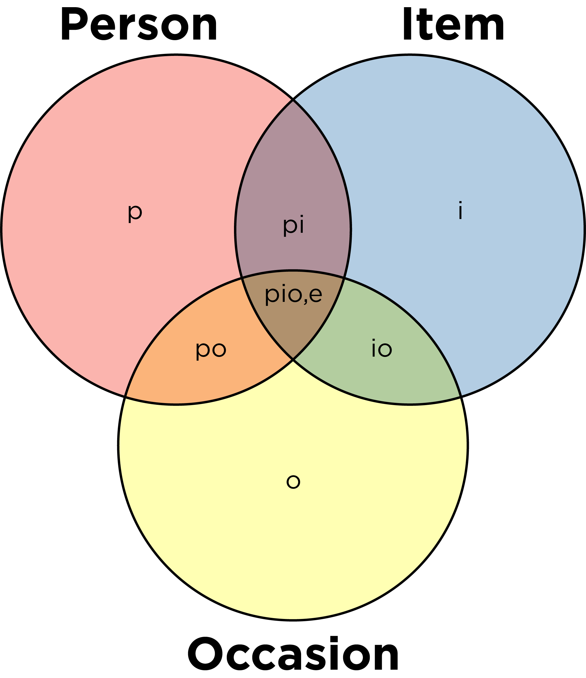
Figure 6.1: Venn Diagram of Variance Components from a Generalizability Theory Model with Person, Item, and Occasion Facets. e refers to the residual. Adapted from https://wmmurrah.github.io/AdvancedMeasurementTheoryNotebook/generalizability.html (archived at https://perma.cc/2EXS-R9MN).
| Source | Variance Accounted For (%) |
|---|---|
| Person (p) | 30 |
| Item (i) | 5 |
| Occasion (o) | 3 |
| p x i | 25 |
| p x o | 5 |
| i x o | 2 |
| p x i x o | 10 |
| residual | 20 |
A score’s usefulness largely depends on the extent to which it allows us to generalize accurately to behavior in a wider set of situations—i.e., a universe of generalization. The G-Theory equivalent of the CTT reliability coefficient of a measure is the generalizability coefficient or dependability coefficient.
6.1.4 G-Theory Perspective on Validity
G-theory can simultaneously consider multiple aspects of reliability and validity in the same model. For instance, internal consistency reliability, test–retest reliability, inter-rater reliability, parallel-forms reliability, and convergent validity (in the D. T. Campbell & Fiske, 1959 sense of the same construct assessed by a different method) can all be incorporated into a G-theory model.
For example, a G-theory model could assess each participant across the following facets:
- time: e.g., T1 and T2 (test–retest reliability)
- items: e.g., questions within the same instrument (internal consistency reliability) and questions across different instruments (parallel-forms reliability)
- rater: e.g., self-report and other-report (inter-rater reliability)
- method: e.g., questionnaire and observation (convergent validity)
Using such a G-theory model, we can determine the extent to which scores on a measure generalize to other conditions, measures, etc. Measures with strong convergent validity show a high ratio of variance as a function of the person relative to the variance as a function of measurement method. To the extent that variance in scores is attributable to different measurement methods, convergent validity is weakened.
An example data structure that could leverage G-theory to partition the variance in scores as a function of different facets (person, time, item, rater, method) and their interactions is in Table 6.2.
| Person | Time | Item | Rater | Method | Score |
|---|---|---|---|---|---|
| 1 | 1 | “hits others” | 1 | questionnaire | 10 |
| 1 | 1 | “hits others” | 1 | observation | 15 |
| 1 | 1 | “hits others” | 2 | questionnaire | 8 |
| 1 | 1 | “hits others” | 2 | observation | 13 |
| 1 | 1 | “argues” | 1 | questionnaire | 4 |
| 1 | 1 | “argues” | 1 | observation | 2 |
| 1 | 1 | “argues” | 2 | questionnaire | 5 |
| 1 | 1 | “argues” | 2 | observation | 7 |
| 1 | 2 | “hits others” | 1 | questionnaire | 8 |
| 1 | 2 | “hits others” | 1 | observation | 10 |
| 1 | 2 | “hits others” | 2 | questionnaire | 6 |
| 1 | 2 | “hits others” | 2 | observation | 7 |
| 1 | 2 | “argues” | 1 | questionnaire | 2 |
| 1 | 2 | “argues” | 1 | observation | 2 |
| 1 | 2 | “argues” | 2 | questionnaire | 4 |
| 1 | 2 | “argues” | 2 | observation | 6 |
| 2 | 1 | “hits others” | 1 | questionnaire | 5 |
| … | … | … | … | … | … |
In sum, G-theory can be a useful way of estimating the degree of reliability and validity of a measure’s scores in the same model.
6.1.5 Generalizability Study
In G-theory, the goal is to conduct a generalizability study (G study) and a decision study (D study). A generalizability study examines the extent of variance in the scores that is attributable to various facets. The researcher must specify and define the universe (set of conditions) to which they would like to generalize their observations and in which they would like to study the reliability of the measure. For instance, it might involve randomly sampling from within that universe in terms of people, items, observers, conditions, timepoints, measurement methods, etc.
6.1.6 Decision Study
After conducting a generalizability study, one can then use the estimates of the extent of variance in scores that are attributable to various facets (estimated from the generalizability study) to conduct a decision study (D study). A decision study examines how generalizable scores from a particular test are if the test is administered in different situations. In G-theory, reliability is estimated with the generalizability coefficient and the dependability coefficient.
6.1.7 Analysis Approach
Traditionally, a generalizability theory approach would test the generalizability study and decision study using a factorial analysis of variance [ANOVA; Brennan (1992)], as exemplified in Section 6.2.4.1, (as opposed to simple ANOVA in CTT). However, ANOVA is limiting—it works best with balanced designs, such as with the same sample size in each condition/facet; but in most real-world applications, data are not equally balanced in each condition. So, it is better to fit G-theory models in a mixed model framework, as exemplified in Section 6.2.4.2.
6.1.8 Practical Challenges
G-theory is strong theoretically, but it has not been widely implemented. G-theory can be challenging because the researcher must specify, define, and assess the universe to which they would like to generalize their observations and to understand the reliability of the measure. Moreover, G-theory has had limited impact because of its omission of a latent variable framework (Dumenci, 2024) (such as in factor analysis, structural equation modeling, and item response theory), which is particularly useful in psychology because the most widely studied constructs in psychology tend to be latent and not directly observable.
6.2 Getting Started
6.2.1 Load Libraries
Code
library("petersenlab") #to install: install.packages("remotes"); remotes::install_github("DevPsyLab/petersenlab")
library("gtheory") #to install: install.packages("https://cran.r-project.org/src/contrib/Archive/gtheory/gtheory_0.1.2.tar.gz")
library("MOTE")
library("tidyverse")
library("tinytex")
library("knitr")
library("rmarkdown")
library("bookdown")
6.2.2 Prepare Data
6.2.2.1 Generate Data
For reproducibility, we set the seed below. Using the same seed will yield the same answer every time. There is nothing special about this particular seed.
6.2.2.2 Add Missing Data
Adding missing data to dataframes helps make examples more realistic to real-life data and helps you get in the habit of programming to account for missing data.
6.2.2.3 Combine Data into Dataframe
Below are examples implementing G-theory.
The pio_cross_dat data file for these examples comes from the gtheory package (Moore, 2016).
The examples are adapted from Huebner & Lucht (2019).
6.2.3 Universe Score for Each Person
Universe scores for each person are generated using the following syntax and are presented in Table ??.
6.2.4 Generalizability (G) Study
Generalizability studies can be conducted in an ANOVA or mixed model framework. Below, we fit a generalizability study model in each framework. In these models, the item, person, and their interaction appear to be the three facets that account for the most variance in scores. Thus, when designing future studies, it would be important to assess and evaluate these facets.
6.2.4.1 ANOVA Framework
                     Df Sum Sq Mean Sq
Person                5 112.95   22.59
Item                  3 119.16   39.72
Occasion              1  14.17   14.17
Person:Item          15  35.61    2.37
Person:Occasion       5   6.58    1.32
Item:Occasion         3   2.26    0.75
Person:Item:Occasion 14  12.08    0.86
1 observation deleted due to missingness
6.2.4.2 Mixed Model Framework
The mixed model framework for estimating generalizability is described by Jiang (2018).
Code
Linear mixed model fit by REML ['lmerMod']
Formula: Score ~ 1 + (1 | Person) + (1 | Item) + (1 | Occasion) + (1 |
    Person:Occasion) + (1 | Person:Item) + (1 | Occasion:Item)
   Data: pio_cross_dat

REML criterion at convergence: 174.7

Scaled residuals:
     Min       1Q   Median       3Q      Max
-1.30232 -0.65304 -0.05246  0.63558  1.37019

Random effects:
 Groups          Name        Variance Std.Dev.
 Person:Item     (Intercept) 0.787305 0.88730
 Person:Occasion (Intercept) 0.117284 0.34247
 Occasion:Item   (Intercept) 0.001574 0.03967
 Person          (Intercept) 2.478043 1.57418
 Item            (Intercept) 3.123803 1.76743
 Occasion        (Intercept) 0.536633 0.73255
 Residual                    0.837426 0.91511
Number of obs: 47, groups:
Person:Item, 24; Person:Occasion, 12; Occasion:Item, 8; Person, 6; Item, 4; Occasion, 2

Fixed effects:
            Estimate Std. Error t value
(Intercept)    5.957      1.234   4.827
Code
$components
           source         var percent n
1     Person:Item 0.787305090    10.0 1
2 Person:Occasion 0.117284076     1.5 1
3   Occasion:Item 0.001573802     0.0 1
4          Person 2.478043107    31.4 1
5            Item 3.123803216    39.6 1
6        Occasion 0.536633200     6.8 1
7        Residual 0.837426163    10.6 1

attr(,"class")
[1] "gstudy" "list"
6.2.5 Decision (D) Study
The decision (D) study and generalizability (G) study, from which the generalizability and dependability coefficients can be estimated, were analyzed using the gtheory package (Moore, 2016).
6.2.6 Generalizability Coefficient
The generalizability coefficient is analogous to the reliability coefficient in CTT. It divides the estimated person variance component (the universe score variance) by the estimated observed-score variance (with some adjustment for the number of observations). In other words, variance in a reliable measure should mostly be due to person variance rather than variance as a function of items, occasion, raters, methods, or other factors. The generalizability coefficient uses relative error variance, so it characterizes the similarity in the relative standing of individuals, similar to CTT-based estimates of relative reliability, such as Cronbach’s alpha. Thus, the generalizability coefficient is an index of relative reliability. The generalizability coefficient ranges from 0–1, and higher scores reflect better reliability.
[1] 0.87310696.2.7 Dependability Coefficient
The dependability coefficient is similar to the generalizability coefficient; however, it uses absolute error variance rather than relative error variance in the estimation. The dependability coefficient characterizes the absolute magnitude of differences across scores, not (just) the relative standing of individuals. Thus, the dependability coefficient is an index of absolute reliability. The dependability coefficient ranges from 0–1, and higher scores reflect better reliability.
[1] 0.63741356.3 Conclusion
G-theory provides an important reminder that reliability is not one thing. You cannot just say that a test “is reliable”; it is important to specify the facets across which the reliability and validity of a measure have been established (e.g., times, raters, items, groups, instruments). Generalizability theory can be a useful way of estimating multiple aspects of reliability and validity of measures in the same model.
6.4 Suggested Readings
Brennan (2001)
6.5 Exercises
6.5.1 Questions
- You want to see how generalizable the Antisocial Behavior subscale of the BPI is. You conduct a generalizability study (“\(G\) study”) to see how generalizable the scores are across participants (\(N = 3\)), two measurement occasions, and three raters. What is the universe score (estimate of true score) for each participant? What percent of variance is attributable to: (a) individual differences among participants, (b) different raters, (c) the measurement occasions, and (d) the interactive effect of raters and measurement occasions? Using a decision study (“\(D\) study”), what are the generalizability and dependability coefficients? Is the measure reliable across the universe (range of factors) we examined it in? Interpret the results from the G study and D study. The data from your study are in Table 6.3 below:
| Participant | Occasion | Rater | Score |
|---|---|---|---|
| 1 | 1 | 1 | 7 |
| 2 | 1 | 1 | 2 |
| 3 | 1 | 1 | 0 |
| 1 | 2 | 1 | 10 |
| 2 | 2 | 1 | 5 |
| 3 | 2 | 1 | 1 |
| 1 | 1 | 2 | 8 |
| 2 | 1 | 2 | 3 |
| 3 | 1 | 2 | 1 |
| 1 | 2 | 2 | 11 |
| 2 | 2 | 2 | 6 |
| 3 | 2 | 2 | 1 |
| 1 | 1 | 3 | 6 |
| 2 | 1 | 3 | 2 |
| 3 | 1 | 3 | 4 |
| 1 | 2 | 3 | 12 |
| 2 | 2 | 3 | 6 |
| 3 | 2 | 3 | 5 |
6.5.2 Answers
- The universe score is \(9\), \(4\), and \(2\) for participants 1, 2, and 3, respectively. The percent of variance attributable to each of those factors is: (a) participant: \(64.6\%\), (b) rater: \(0.2\%\), (c) the measurement occasion: \(16.2\%\), and (d) the interactive effect of rater and measurement occasion: \(1.5\%\). The generalizability coefficient is \(.90\), and the dependability coefficient is \(.81\). The measure is fairly reliable across the universe examined, both in terms of relative differences (generalizability coefficient) and absolute differences (dependability coefficient). However, when using the measure in future work, it would be important to assess many participants (due to the strong presence of individual differences) across multiple occasions (due to the strong effect of occasion) and multiple raters (due to the moderated effect of rater as a function of participant). It will be important to account for the considerable sources of variance in scores on the measure in future work including: participant, occasion, participant \(\times\) rater, and participant \(\times\) occasion. By accounting for these sources of variance, we can get a purer estimate of each participant’s true score and the population’s true score.