I want your feedback to make the book better for you and other readers. If you find typos, errors, or places where the text may be improved, please let me know. The best ways to provide feedback are by GitHub or hypothes.is annotations.
Opening an issue or submitting a pull request on GitHub: https://github.com/isaactpetersen/Principles-Psychological-Assessment
Adding an annotation using hypothes.is.
To add an annotation, select some text and then click the
symbol on the pop-up menu.
To see the annotations of others, click the
symbol in the upper right-hand corner of the page.
Chapter 21 Computers and Adaptive Testing
21.1 Computer-Administered/Online Assessment
Computer-administered and online assessments have the potential to be both desirable and dangerous (Buchanan, 2002). The potential is to have a mental health screening instrument online that a person fills out, is automatically scored, and automatic feedback is provided with suggestions to follow a particular course of action. This would save the clinician time and could lead to a more productive therapy session. As an example, I have clients complete a brief measure of behavioral issues on a tablet when they arrive and are waiting in the waiting room. This is an example of measurement-based care, in which the participant’s treatment response is assessed throughout treatment to help determine whether treatment is working or not, and whether to try something different. In addition, emerging techniques in machine learning may be useful for scoring of high-dimensional data in assessment in clinical practice (Galatzer-Levy & Onnela, 2023).
21.1.1 Advantages
There are many advantages of computer-administered or online assessment:
- Computer-administered and online assessment requires less time on the part of the clinician and administrators than traditional assessment methods. They do not need the clinician to administer and score the assessment, and scores can be entered directly into the client’s chart.
- Computer-administered and online assessments tend to be less costly than traditional assessment methods.
- Computer-administered and online assessments can increase access to services because some people can complete the assessment who otherwise would not be able to complete it. For example, some people may be restricted by geographic or financial circumstances. You can provide the questionnaire in multiple languages and modalities, including written, spoken, and pictorial.
- People may disclose more information to a computer than to a person. The degree of one’s perceived anonymity matters. Perceived anonymity may be especially important for information on sensitive yet important issues, such as suicidality, homicidality, abuse, neglect, criminal behavior, etc.
- Computerized and online assessment has the potential to be more structured and the potential to do a more comprehensive and accurate assessment than an in-person interview, which tends to be less structured and more biased by clinical judgment (Garb, 2007).
- Computerized and online assessment tends to provide more comprehensive information than is usually collected in practice. Structured approaches tend to ask more questions. Computers can increase the likelihood that the client answers all questions, because it can prevent clients from skipping questions. Computers can apply “branching logic” to adapt which questions are asked based on the participant’s responses (i.e., adaptive testing) to more efficiently gain greater coverage. Clinicians tend not to ask questions about important issues. Clinicians fail to examine disorders other than the hypothesized ones, which is known as diagnostic overshadowing due to the confirmation bias of looking for evidence-confirming information rather than disconfirming evidence. In general, computers give more diagnoses than clinicians. Clinicians often miss co-occurring disorders. Doing a more comprehensive assessment normalizes that people can and do experience the behavioral issues that they are asked about, and can increase self-disclosure. Greater structure leads to higher inter-rater reliability, less bias, and greater validity.
- Computerized and online assessment lends itself to continuous monitoring during treatment for measurement-based care. Measurement-based care has been shown to be related to better treatment outcomes. Computerized or online assessment may be important in risk assessment that might otherwise go unrecognized. Treatment utility of computerized assessment has been demonstrated for suicide and substance use.
21.1.2 Validity Challenges
There are a number of challenges to the validity of computer-administered and online assessment:
- The impersonality of computers; however, this does not seem to be a strong threat.
- Lack of control in the testing situation.
- The possibility that extraneous factors can influence responses.
- Language and cultural differences; it is difficult to ask follow-up questions to assess understanding unless a clinician is present.
- Inability to observe the client’s body language or nonverbals.
- Computers are not a great medium to assess constructs that could be affected by computer-related anxiety.
- Some constructs show different ratings online versus in-person.
- Computer-administered and online assessment may require different norms and cutoffs than paper-and-pencil assessment. Different norms could be necessary, for example, due to increased self-disclosure and higher ratings of negative affect in computer-administered assessment compared to in-person assessment.
- Careless and fraudulent responding can be common when recruiting an online sample to complete a survey (Chandler et al., 2020). Additional steps may need to be taken to ensure high-quality responses such as CAPTCHA (or reCAPTCHA), internet protocol (IP) verification of location, and attention or validity checks.
In general, online assessments of personality seem generally comparable to their paper-and-pencil versions, but their psychometric properties are not identical. In general, computer-administered and online assessments yield the same factor structure as in-person assessments, but particular items may not function in the same way across computer versus in-person assessments.
21.1.3 Ethical Challenges
There are important ethical challenges of using computer-administered and online assessments:
- The internet and app stores provide a medium for the dissemination and proliferation of quackery. Businesses sell access to assessment information despite no evidence of the reliability or validity of the measure.
- When giving potentially distressing or threatening feedback, it is important to provide opportunities for follow-up sessions or counseling. When using online assessment in research, you can state that release of test scores is not possible, and that participants should consult a professional if they are worried or would like a professional assessment.
- An additional ethical challenge of computer-administered and online assessment deals with test security. The validity of many tests is based on the assumption that the client is not knowledgeable about the test materials. Detailed information on many protected tests is available on the internet (Ruiz et al., 2002), and it could be used by malingerers to fake health or illness.
- Data security is another potential challenge of computer-administered and online assessments, including how to protect HIPAA compliance in the clinical context.
21.1.4 Best Practices
Below are best practices for computer-administered and online assessments:
- Only use measures with established reliability and validity, unless you are studying them, in which case you should evaluate their psychometrics.
- Have a trained clinician review the results of the assessment.
- Combine computer-administered assessment with clinical judgment. Clients can be expected to make errors completing the assessment, so ask necessary follow-up questions after getting results from computer-administered assessments. Asking follow-up questions can help avoid false positive errors in diagnosis. Check whether a client mistakenly reported something; or whether they under-/over-reported psychopathology.
- Provide opportunities for follow-up sessions or counseling if distressing or threatening feedback is provided.
- It may be important to correct for a person’s level of experience with computers when using computerized tasks for clinical decision-making (Lee Meeuw Kjoe et al., 2021).
21.2 Adaptive Testing
Adaptive testing involves having the respondent complete only those items that are needed to answer an assessment question. It involves changing which items are administered based on responses to previous items, and administering only a subset of the possible items. Adaptive testing is commonly used in intelligence testing, achievement testing, and aptitude testing. Adaptive testing is not yet commonly used for personality or psychopathology assessment. Most approaches to assessment of personality and psychopathology rely on conventional testing approaches using classical test theory. But many structured clinical interviews, use decision rules to skip a diagnosis, module, or section if a decision rule is not met. Adaptive testing has also been used with observational assessments (e.g., Granziol et al., 2022).
A goal of adaptive testing is to get the most accurate estimate of a person’s level on a construct with the fewest items possible. Ideally, you would get similar results between adaptive testing and conventional testing that uses all items, when adaptive testing is done well.
There are multiple approaches to adaptive testing. Broadly, one class of approaches uses manual administration, whereas another class of approaches uses computerized adaptive testing (CAT) based on item response theory (IRT).
21.2.1 Manual Administration of Adaptive Testing (Adaptive Testing without IRT)
Manual administration of adaptive testing involves moving people up and down in the item difficulty according to their responses. Approaches to manual administration of adaptive testing include using skip rules, basal and ceiling criteria, and the countdown method.
21.2.1.1 Skip Rules
Many structured clinical interviews, such as the Structured Clinical Interview for DSM Disorders (SCID) and Mini-International Neuropsychiatric Interview (MINI), use decision rules to skip a diagnosis, module, or section if a decision rule is not met. The skip rules allow the interviews to be more efficient and therefore clinically practical.
21.2.1.2 Basal and Ceiling Approach
One approach to manual administration of adaptive testing involves establishing a respondent’s basal and ceiling level. The basal level is the difficulty level at which the examinee answers almost all items correctly. The respondent’s ceiling level is the difficulty level at which the examinee answers almost all items incorrectly. The basal and ceiling criteria set the rules for establishing the basal and ceiling level for each respondent and for when to terminate testing.
The goal of adaptive testing is to administer the fewest items necessary to get an accurate estimate of the person’s ability, to save time and prevent the respondent from becoming bored from too-easy items or frustrated from too-difficult items. The basal and ceiling approach starts testing at the recommended starting point for a person’s age or ability level. The examiner scores as items are administered. If the person gets too many items wrong in the beginning, the examiner moves to an earlier starting point, i.e., provides easier items, until the respondent gets most items correct, which establishes their basal level. Then, after establishing the respondent’s basal level, the examiner proceeds forward to progressively more difficult items until they reach their ceiling level, i.e., they get too many wrong in some set, which establishes their ceiling level.
21.2.1.3 Countdown Approach
The countdown approach of adaptive testing is a variant of the variable termination criterion approach to adaptive testing. It classifies the respondent into one of two groups—elevated or not elevated—based on whether they exceed the cutoff criterion on a given scale. The cutoff criterion is usually the raw score on the scale that corresponds to a clinical elevation.
Two countdown approaches include (1) the classification method and (2) the full scores on elevated scales (FSES) method. The countdown approach to adaptive testing is described by Forbey & Ben-Porath (2007).
21.2.1.3.1 Classification Method
Using the classification method to the countdown approach of adaptive testing, the examiner stops administering items once elevation is either ruled in or ruled out. The classification method only tells you whether a client produced an elevated score on the scale. It does not tell you their actual score on that scale.
21.2.1.3.2 Full Scores on Elevated Scales Method
Using the full scores on elevated scales method to the countdown approach of adaptive testing, the examiner stops administering items only if elevation is ruled out. The approach generates a score on that scale only for people who produced an elevated score.
21.2.1.4 Summary
When doing manual administration with clinical scales, you see the greatest item savings when ordering items from least to most frequently endorsed (i.e., from most to least difficulty) so you can rule people out faster. Ordering items in this way results in a 20–30% item savings on the Minnesota Multiphasic Personality Inventory (MMPI), and corresponding time savings. Comparative studies using the MMPI tend to show comparable results (i.e., similar validity) between the countdown adaptive method and the conventional testing method. That is, the reduction in items does not impair the validity of the adaptive scales. However, you can get even greater item savings when using an IRT approach to adaptive testing. Using IRT, you can order the administration of items differently for each participant to administer the next item that will provide the most information (i.e., precision) for a respondent’s ability given their responses on all previous items.
21.2.2 CAT with IRT
Computerized adaptive testing (CAT) based on IRT is widely used in educational testing, including the Graduate Record Examination (GRE) and the Graduate Management Admission Test (GMAT), but it is not widespread in mental health measurement for two reasons: (1) it works best with large item banks; large item banks are generally unavailable for mental health constructs; and (2) mental health constructs are multidimensional and CAT using IRT has primarily been restricted to unidimensional constructs, such as math achievement. However, that is changing; there are now multidimensional IRT approaches that allow simultaneously estimating people’s scores on multiple dimensions, as described in Section 8.6. For example, the higher-order construct of externalizing problems includes sub-dimensions including aggression and rule-breaking.
A CAT is designed to locate a person’s level on the construct (theta) with as few items as possible. CAT has potential for greater item savings than the countdown approach, but it has more assumptions. IRT can be used to create CATs using information gleaned from the IRT model’s item parameters, including discrimination and difficulty (or severity). The item’s discrimination indicates how strongly the item is related to the construct. For a strong measure, you want highly discriminating items that are strongly related to the construct. In terms of item difficulty/severity, you want items that span the full distribution of difficulty/severity so they are non-redundant.
An IRT-based CAT starts with a highly discriminating item at the 50th percentile of the distribution (severity) (or at whatever level is the best estimate of the person’s ability/severity before the CAT is administered). Then, based on the participant’s response, it generates a provisional estimate of the person’s level on the construct and administers the item that will provide the most information. For example, if the respondent gets the first item correct, the CAT administers a highly discriminating item that might be at the 75th percentile of the distribution (severity). And so on, based on the participants’ responses.
As described in Section 8.1.6, item information is how much measurement precision for the construct is provided by a particular item. In other words, item information indicates how much the item reduces the standard error of measurement; i.e., how much the item reduces uncertainty of our estimate of the respondent’s construct level. An IRT-based CAT continues to generate provisional estimates of the person’s construct level and updates it based on new responses. The CAT tries to find the construct level where the respondent keeps getting items right and wrong (or endorsing versus not endorsing) 50% of the time. This process continues until the uncertainty in the person’s estimated construct level is smaller than a pre-defined threshold—that is, when we are fairly confident (to some threshold) about a person’s construct level.
CAT is a promising approach that saves time because it tailors which items are administered to which person and in which order based on their construct level to get the most reliable estimate in the shortest time possible. It administers items that are appropriate to the person’s construct level, and it does not administer items that are way too easy or way too hard for the person, which saves time, boredom, and frustration. It shortens the assessment because not all items are administered, and it typically results in around 50% item savings or more. It also allows for increased measurement precision, because you are drilling down deeper (i.e., asking more items) near the person’s construct level. You can control the measurement precision of the CAT because you can specify the threshold of measurement precision (i.e., standard error of measurement) at which testing is terminated. For example, you could have the CAT terminate when the standard error of measurement of a person’s construct level becomes less than 0.2.
However, CATs assume that if you get a more difficult item correct, you would have gotten easier items correct, which might not be true in all contexts (especially for constructs that are not unidimensional). For example, just because a person does not endorse low-severity symptoms does not necessarily mean that they will not endorse higher-severity symptoms, especially when assessing a multidimensional construct.
Simpler CATs are built using unidimensional IRT. But many aspects of psychopathology are not unidimensional, and would violate assumptions of unidimensional IRT. For example, the externalizing spectrum includes sub-dimensions including aggression, disinhibition, and substance use. You can use multidimensional IRT to build CATs, though this is more complicated. For instance, you could estimate a bifactor model in which each item (e.g., “hits others”) loads onto the general latent factor (e.g., externalizing problems) and its specific sub-dimension (e.g., aggression versus rule-breaking). Computerized adaptive testing of mental health disorders is reviewed by Gibbons et al. (2016).
Well-designed CATs show equivalent reliability and validity to their full-scale counterparts. By contrast, many short forms are not as accurate as their full-scale counterparts. Part of the reason that CATs tend to do better than short forms is that the CATs are adaptive; they determine which items to administer based on the participant’s responses to prior items, unlike short forms. For guidelines on developing and evaluating short forms, see Smith et al. (2000).
21.4 Example of Unidimensional CAT
The computerized adaptive test (CAT) was fit using the mirtCAT package (Chalmers, 2021).
The example of a CAT with unidimensional data is adapted from mirtCAT documentation: https://philchalmers.github.io/mirtCAT/html/unidim-exampleGUI.html (archived at https://perma.cc/3ZW4-DAUR)
21.4.1 Define Population IRT Parameters
For reproducibility, we set the seed below. Using the same seed will yield the same answer every time. There is nothing special about this particular seed.
21.4.3 Model Summary
            F1    h2
Item.1   0.673 0.453
Item.2   0.369 0.136
Item.3   0.548 0.300
Item.4   0.500 0.250
Item.5   0.783 0.614
Item.6   0.579 0.335
Item.7   0.733 0.538
Item.8   0.377 0.142
Item.9   0.535 0.286
Item.10  0.503 0.253
Item.11  0.546 0.298
Item.12  0.591 0.349
Item.13  0.630 0.397
Item.14  0.597 0.356
Item.15  0.583 0.340
Item.16  0.389 0.151
Item.17  0.570 0.325
Item.18  0.460 0.211
Item.19  0.683 0.466
Item.20  0.507 0.257
Item.21  0.547 0.300
Item.22  0.581 0.337
Item.23  0.784 0.614
Item.24  0.546 0.298
Item.25  0.551 0.303
Item.26  0.615 0.379
Item.27  0.567 0.321
Item.28  0.554 0.307
Item.29  0.625 0.391
Item.30  0.733 0.537
Item.31  0.737 0.544
Item.32  0.458 0.210
Item.33  0.520 0.271
Item.34  0.575 0.331
Item.35  0.532 0.283
Item.36  0.448 0.201
Item.37  0.481 0.231
Item.38  0.485 0.236
Item.39  0.459 0.210
Item.40  0.656 0.430
Item.41  0.682 0.464
Item.42  0.596 0.355
Item.43  0.682 0.465
Item.44  0.564 0.319
Item.45  0.392 0.154
Item.46  0.538 0.290
Item.47  0.490 0.240
Item.48  0.641 0.411
Item.49  0.519 0.269
Item.50  0.505 0.255
Item.51  0.490 0.240
Item.52  0.530 0.281
Item.53  0.319 0.101
Item.54  0.834 0.695
Item.55  0.643 0.414
Item.56  0.489 0.239
Item.57  0.563 0.317
Item.58  0.538 0.289
Item.59  0.627 0.393
Item.60  0.598 0.357
Item.61  0.480 0.230
Item.62  0.523 0.273
Item.63  0.586 0.343
Item.64  0.650 0.422
Item.65  0.652 0.425
Item.66  0.723 0.522
Item.67  0.447 0.199
Item.68  0.524 0.274
Item.69  0.489 0.239
Item.70  0.783 0.613
Item.71  0.680 0.462
Item.72  0.455 0.207
Item.73  0.452 0.204
Item.74  0.614 0.377
Item.75  0.629 0.396
Item.76  0.595 0.354
Item.77  0.651 0.424
Item.78  0.515 0.265
Item.79  0.671 0.450
Item.80  0.464 0.215
Item.81  0.612 0.375
Item.82  0.491 0.241
Item.83  0.489 0.239
Item.84  0.385 0.148
Item.85  0.455 0.207
Item.86  0.402 0.161
Item.87  0.537 0.288
Item.88  0.651 0.424
Item.89  0.662 0.439
Item.90  0.433 0.188
Item.91  0.562 0.315
Item.92  0.752 0.565
Item.93  0.572 0.328
Item.94  0.518 0.269
Item.95  0.559 0.312
Item.96  0.714 0.509
Item.97  0.714 0.510
Item.98  0.591 0.349
Item.99  0.346 0.120
Item.100 0.443 0.196

SS loadings:  32.822
Proportion Var:  0.328

Factor correlations:

   F1
F1 1$items
a b g u
Item.1 1.549 0.298 0.2 1
Item.2 0.676 0.742 0.2 1
Item.3 1.115 -0.536 0.2 1
Item.4 0.982 -0.448 0.2 1
Item.5 2.145 -0.380 0.2 1
Item.6 1.208 0.409 0.2 1
Item.7 1.836 -0.606 0.2 1
Item.8 0.694 2.000 0.2 1
Item.9 1.077 -0.991 0.2 1
Item.10 0.991 0.570 0.2 1
Item.11 1.109 0.493 0.2 1
Item.12 1.246 0.363 0.2 1
Item.13 1.382 -0.417 0.2 1
Item.14 1.267 0.925 0.2 1
Item.15 1.222 0.405 0.2 1
Item.16 0.718 2.062 0.2 1
Item.17 1.182 -0.233 0.2 1
Item.18 0.881 -0.151 0.2 1
Item.19 1.591 0.647 0.2 1
Item.20 1.000 -0.120 0.2 1
Item.21 1.113 -0.430 0.2 1
Item.22 1.214 -1.437 0.2 1
Item.23 2.146 -0.025 0.2 1
Item.24 1.110 0.204 0.2 1
Item.25 1.123 -0.584 0.2 1
Item.26 1.329 0.127 0.2 1
Item.27 1.171 -0.421 0.2 1
Item.28 1.132 0.136 0.2 1
Item.29 1.363 0.425 0.2 1
Item.30 1.834 0.019 0.2 1
Item.31 1.858 -0.215 0.2 1
Item.32 0.878 1.927 0.2 1
Item.33 1.037 0.396 0.2 1
Item.34 1.197 -0.304 0.2 1
Item.35 1.069 -1.655 0.2 1
Item.36 0.853 0.979 0.2 1
Item.37 0.933 0.799 0.2 1
Item.38 0.945 -0.062 0.2 1
Item.39 0.879 1.319 0.2 1
Item.40 1.477 0.629 0.2 1
Item.41 1.585 0.136 0.2 1
Item.42 1.262 0.913 0.2 1
Item.43 1.587 0.508 0.2 1
Item.44 1.164 -1.134 0.2 1
Item.45 0.725 -0.191 0.2 1
Item.46 1.087 0.724 0.2 1
Item.47 0.957 1.837 0.2 1
Item.48 1.423 0.155 0.2 1
Item.49 1.033 0.892 0.2 1
Item.50 0.996 -0.109 0.2 1
Item.51 0.958 1.628 0.2 1
Item.52 1.063 0.368 0.2 1
Item.53 0.572 -1.014 0.2 1
Item.54 2.568 0.403 0.2 1
Item.55 1.430 -0.931 0.2 1
Item.56 0.955 -0.193 0.2 1
Item.57 1.160 0.829 0.2 1
Item.58 1.086 0.126 0.2 1
Item.59 1.371 -0.150 0.2 1
Item.60 1.269 0.220 0.2 1
Item.61 0.931 0.868 0.2 1
Item.62 1.044 0.597 0.2 1
Item.63 1.231 -0.278 0.2 1
Item.64 1.455 1.303 0.2 1
Item.65 1.464 -0.644 0.2 1
Item.66 1.780 -0.313 0.2 1
Item.67 0.850 1.466 0.2 1
Item.68 1.046 -1.062 0.2 1
Item.69 0.953 0.441 0.2 1
Item.70 2.141 -0.051 0.2 1
Item.71 1.576 -0.743 0.2 1
Item.72 0.870 -0.833 0.2 1
Item.73 0.862 -0.859 0.2 1
Item.74 1.325 -0.981 0.2 1
Item.75 1.378 -0.196 0.2 1
Item.76 1.259 0.496 0.2 1
Item.77 1.459 0.795 0.2 1
Item.78 1.021 0.834 0.2 1
Item.79 1.539 -0.290 0.2 1
Item.80 0.891 0.943 0.2 1
Item.81 1.319 -0.067 0.2 1
Item.82 0.960 1.233 0.2 1
Item.83 0.953 -1.236 0.2 1
Item.84 0.710 -1.120 0.2 1
Item.85 0.870 0.592 0.2 1
Item.86 0.746 -2.303 0.2 1
Item.87 1.082 -0.205 0.2 1
Item.88 1.460 -0.297 0.2 1
Item.89 1.505 0.138 0.2 1
Item.90 0.819 0.273 0.2 1
Item.91 1.155 0.149 0.2 1
Item.92 1.939 0.153 0.2 1
Item.93 1.188 0.856 0.2 1
Item.94 1.032 -1.256 0.2 1
Item.95 1.147 0.432 0.2 1
Item.96 1.734 -0.289 0.2 1
Item.97 1.737 0.262 0.2 1
Item.98 1.247 -0.538 0.2 1
Item.99 0.628 -0.839 0.2 1
Item.100 0.841 -0.259 0.2 1
$means
F1
0
$cov
F1
F1 121.4.4 Model Plots
A test characteristic curve of the measure is in Figure 21.1.
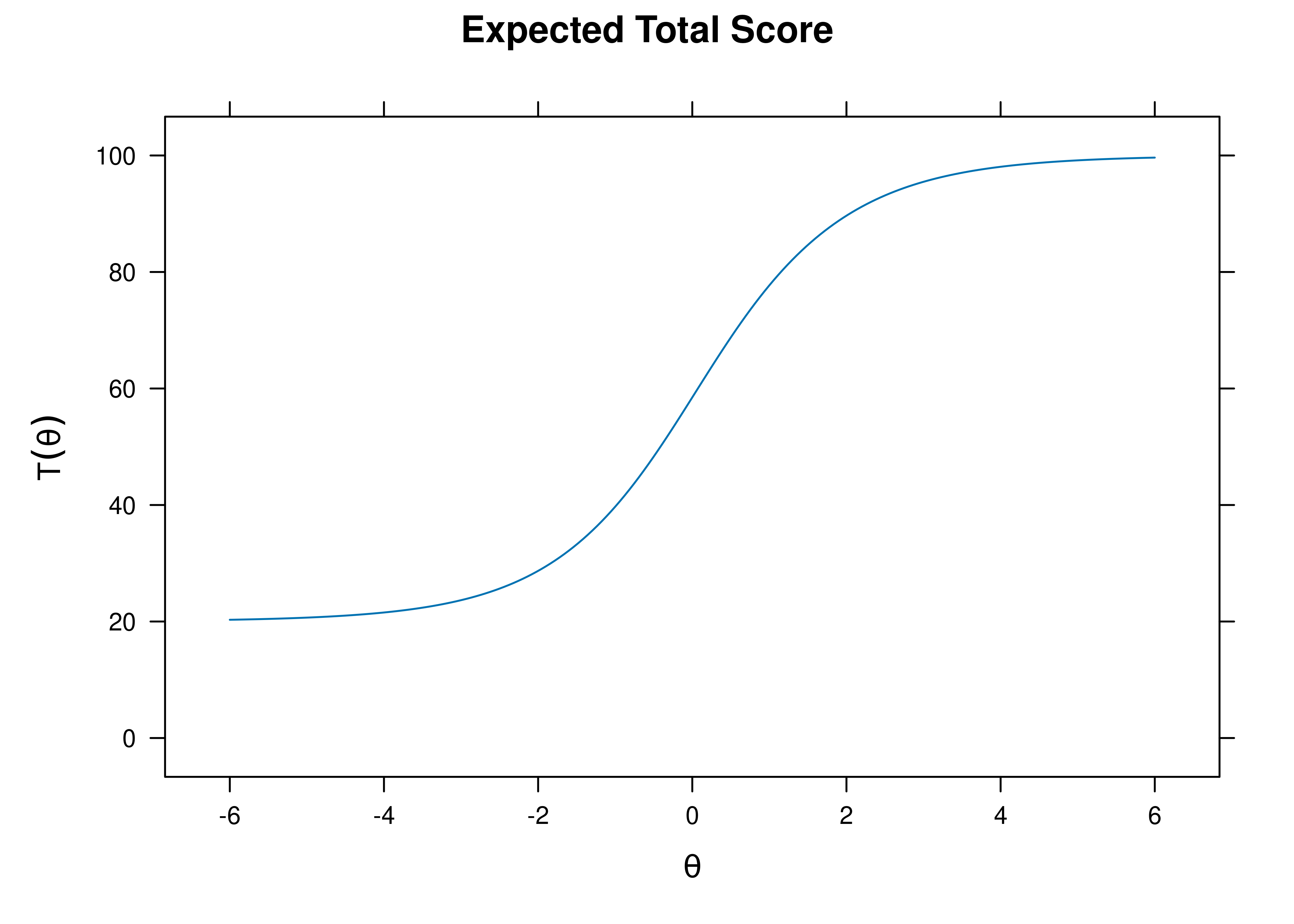
Figure 21.1: Test Characteristic Curve.
The test information and standard error of measurement as a function of the person’s construct level (theta; \(\theta\)) is in Figure 21.2. The test appears to measure theta (\(\theta\)) with \(SE < .4\) within a range of −1.5 to 2.
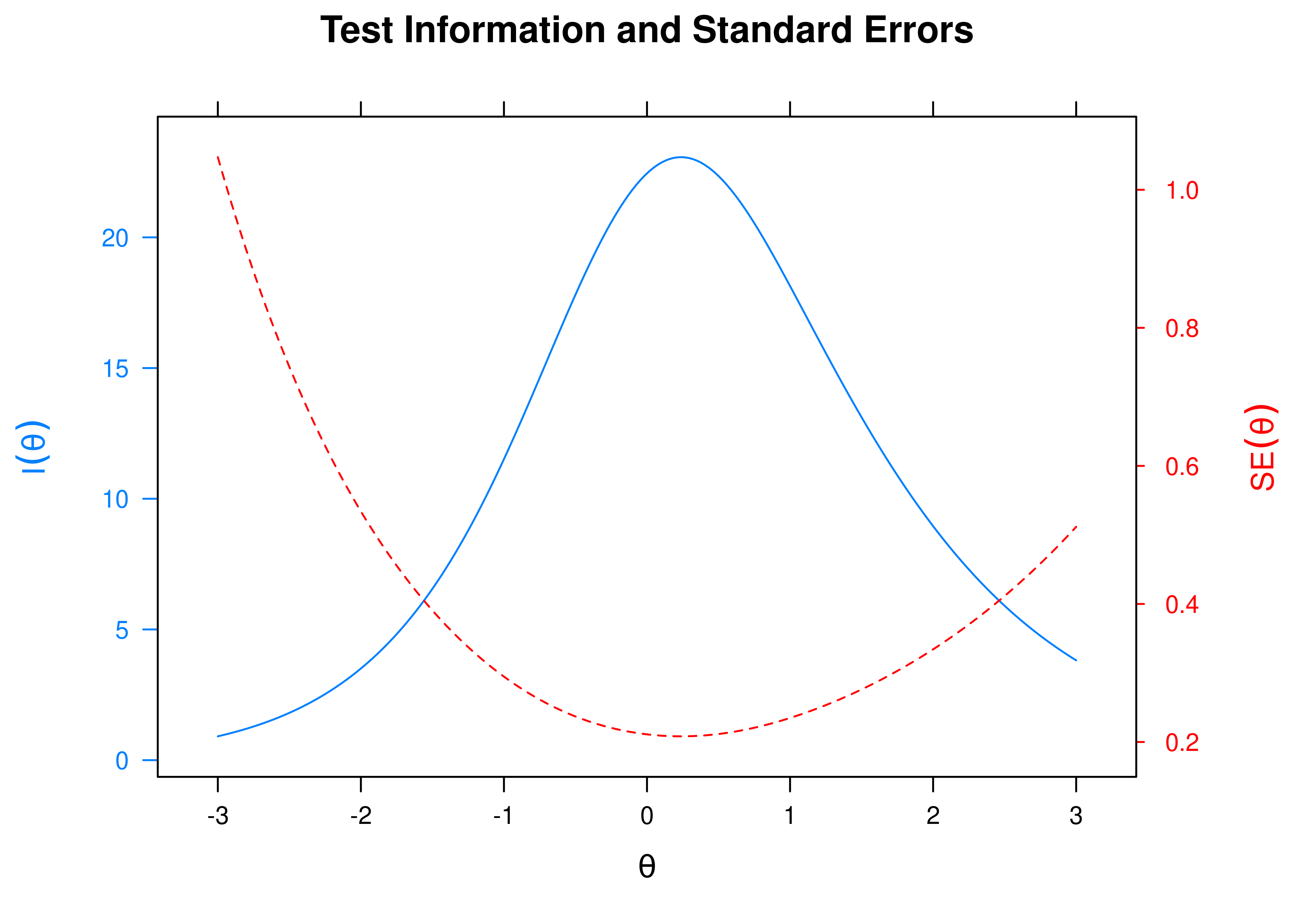
Figure 21.2: Test Information and Standard Error of Measurement.
21.4.5 Item Plots
Item characteristic curves are in Figure 21.3.
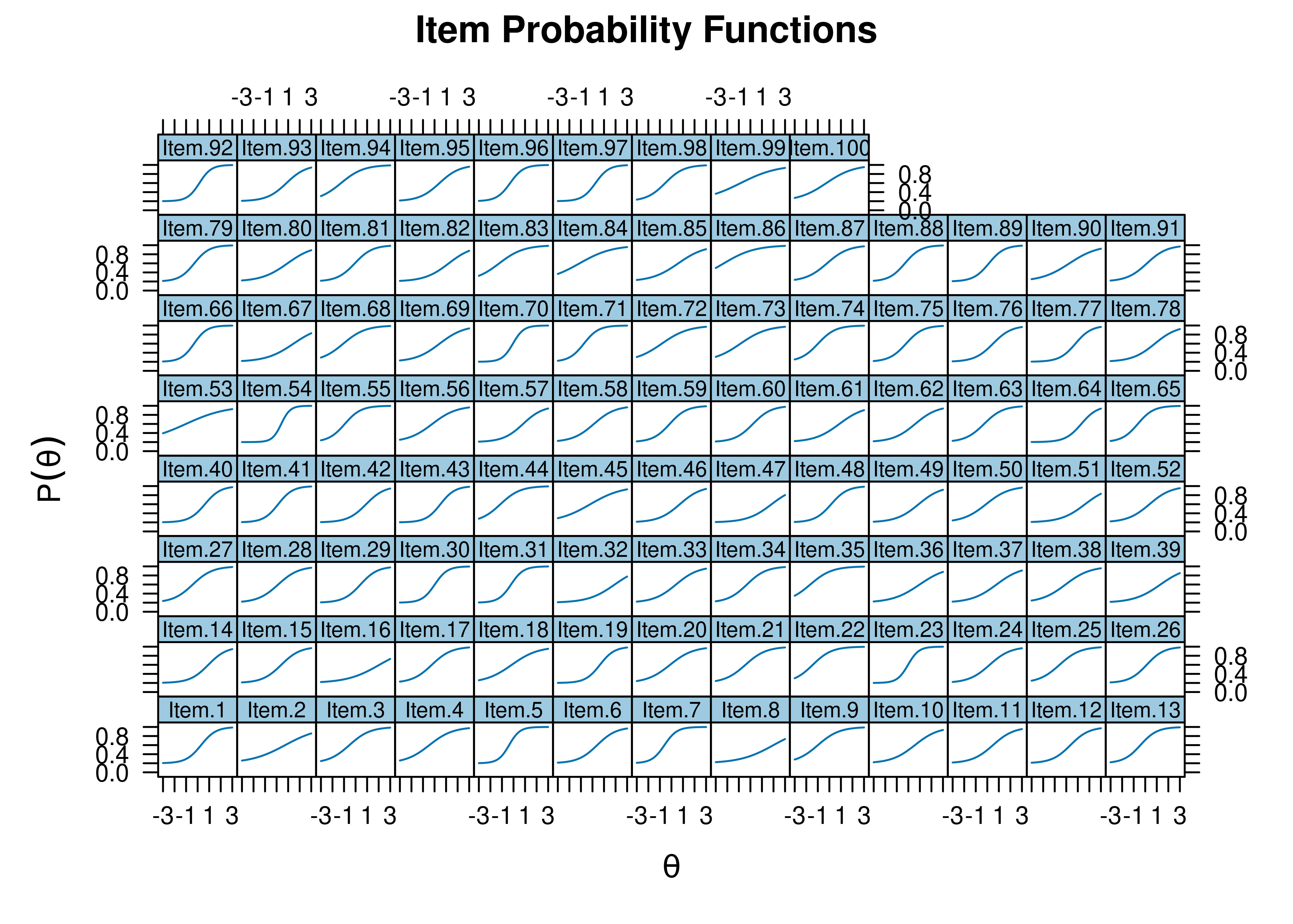
Figure 21.3: Item Characteristic Curves.
Item information curves are in Figure 21.4.
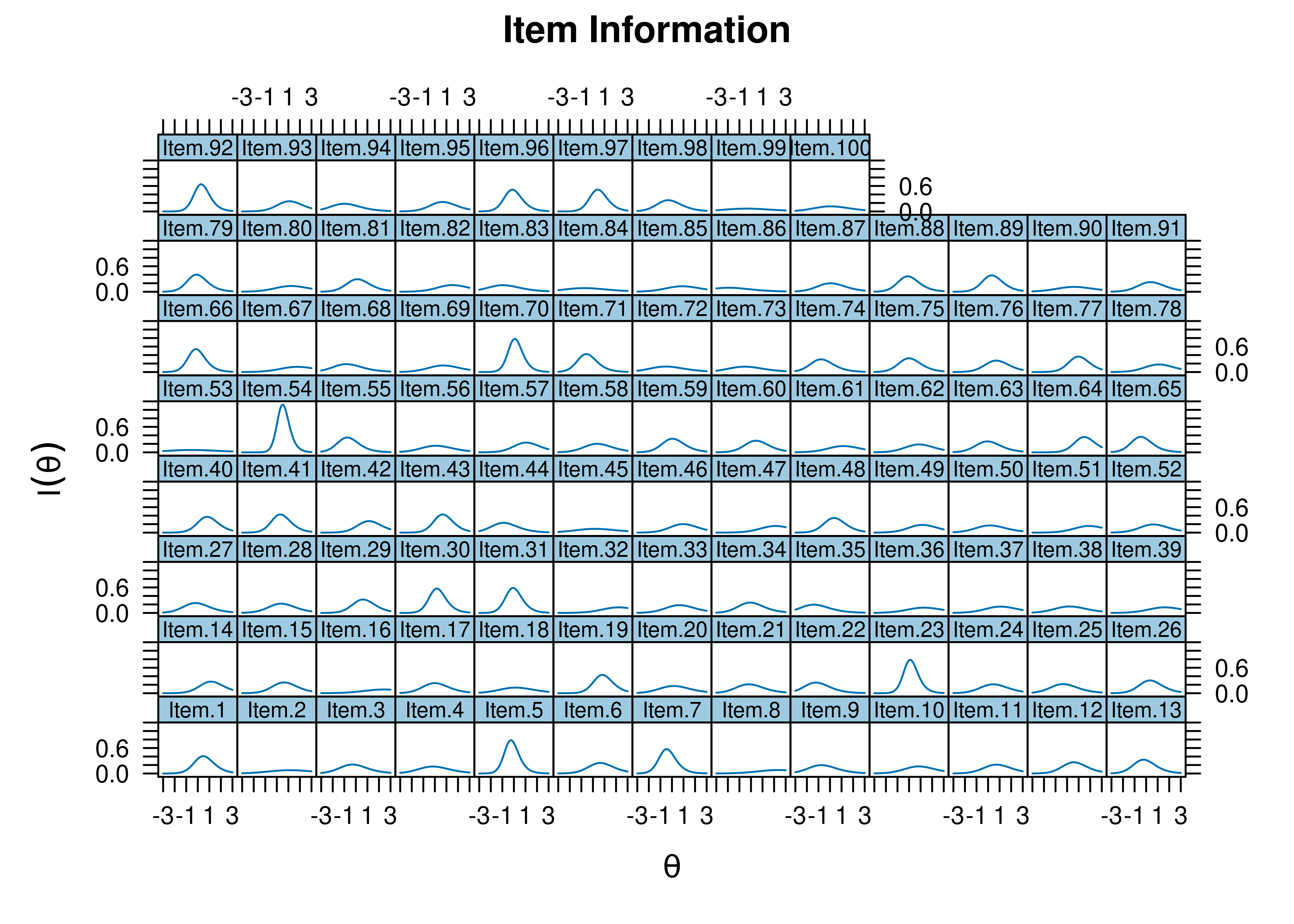
Figure 21.4: Item Information Curves.
- Item 30 would be a good starting item; it has a difficulty closest to the 50th percentile \((b = 0.019)\) and a high discrimination \((a = 1.834)\).
- Item 70 would be a good starting item; it has a difficulty closest to the 50th percentile \((b = -0.051)\) and a high discrimination \((a = 2.141)\).
- Item 86 is an easy item \((b = -2.303)\).
- Item 16 is a difficult item \((b = 2.062)\).
- Item 53 has a low discrimination \((a = 0.572)\).
Item characteristic curves and information curves for these items are in Figures 21.5–21.9.
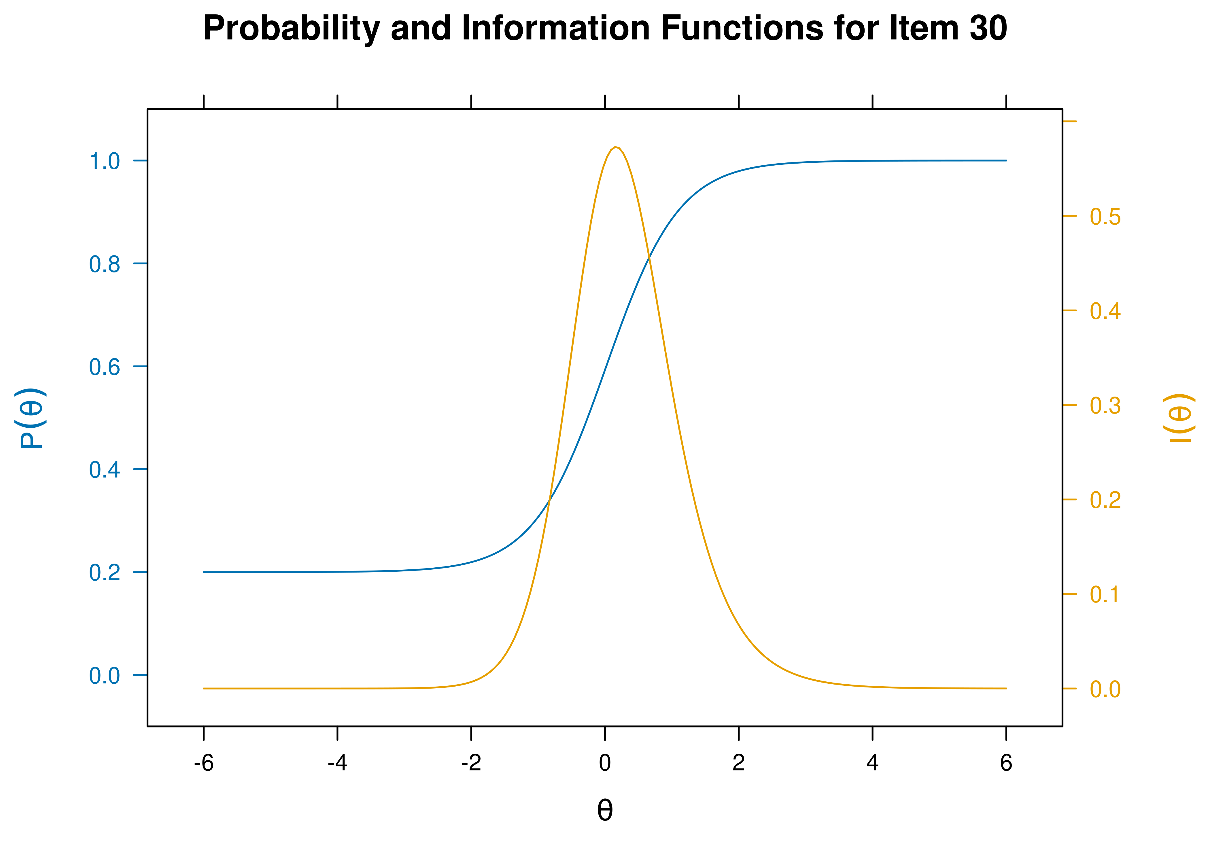
Figure 21.5: Item Characteristic Curves and Information Curves: Item 30.
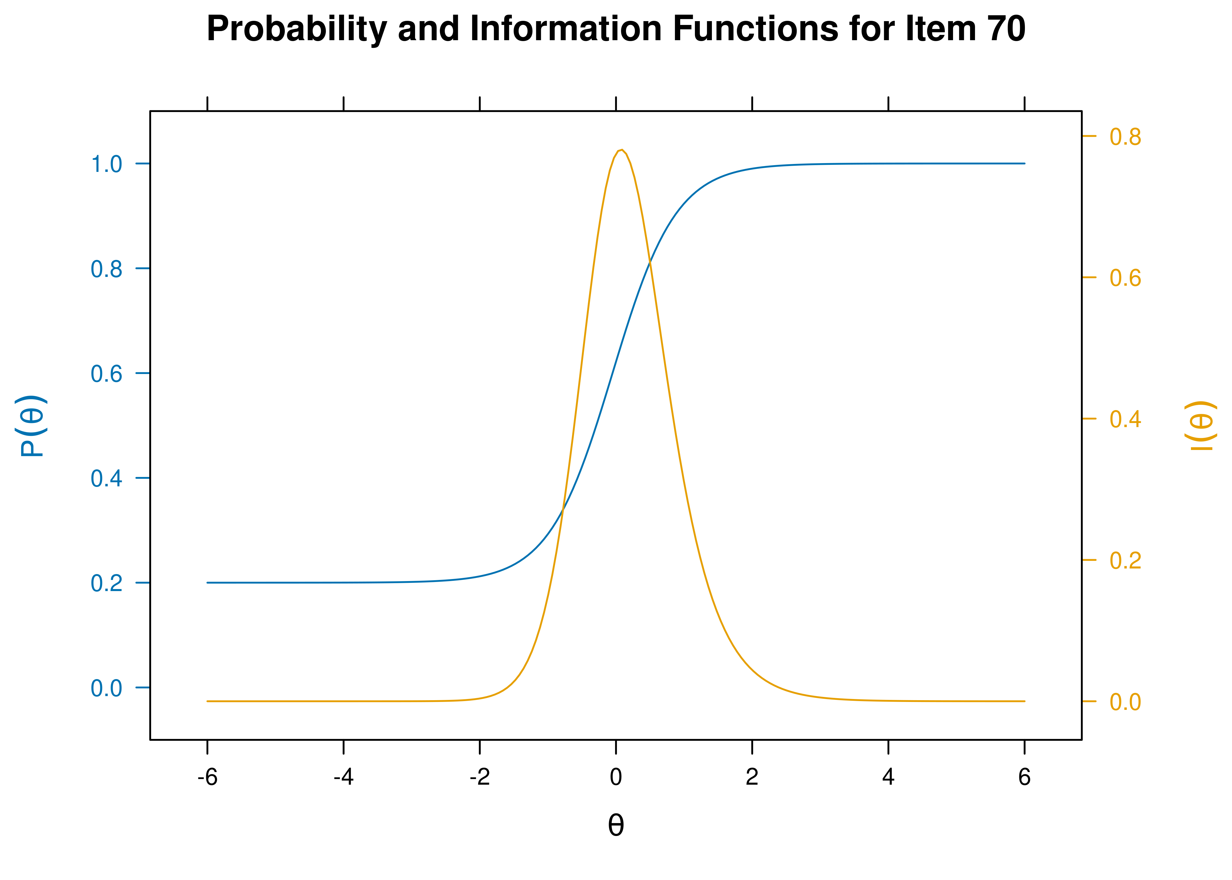
Figure 21.6: Item Characteristic Curves and Information Curves: Item 70.
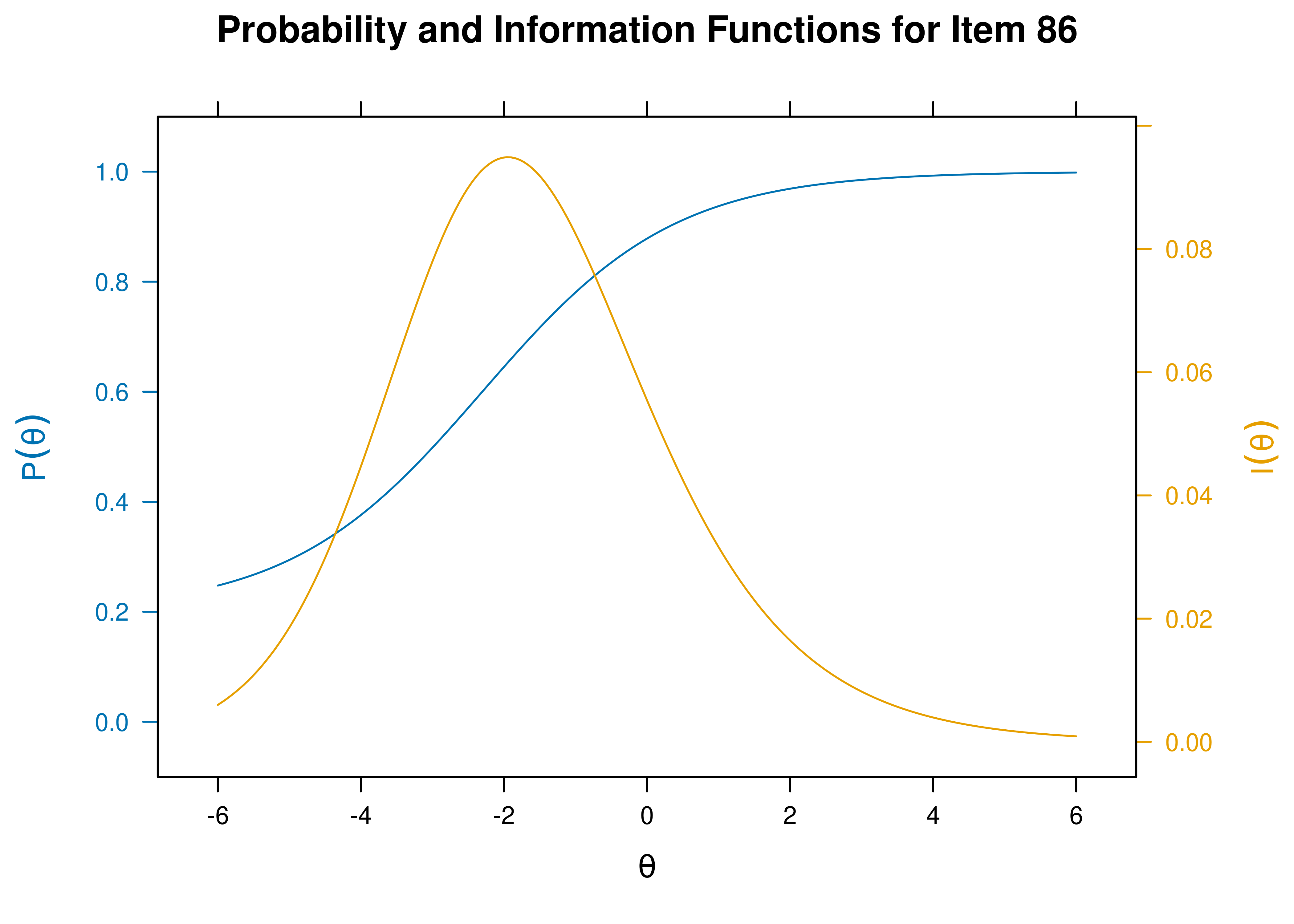
Figure 21.7: Item Characteristic Curves and Information Curves: Item 86.
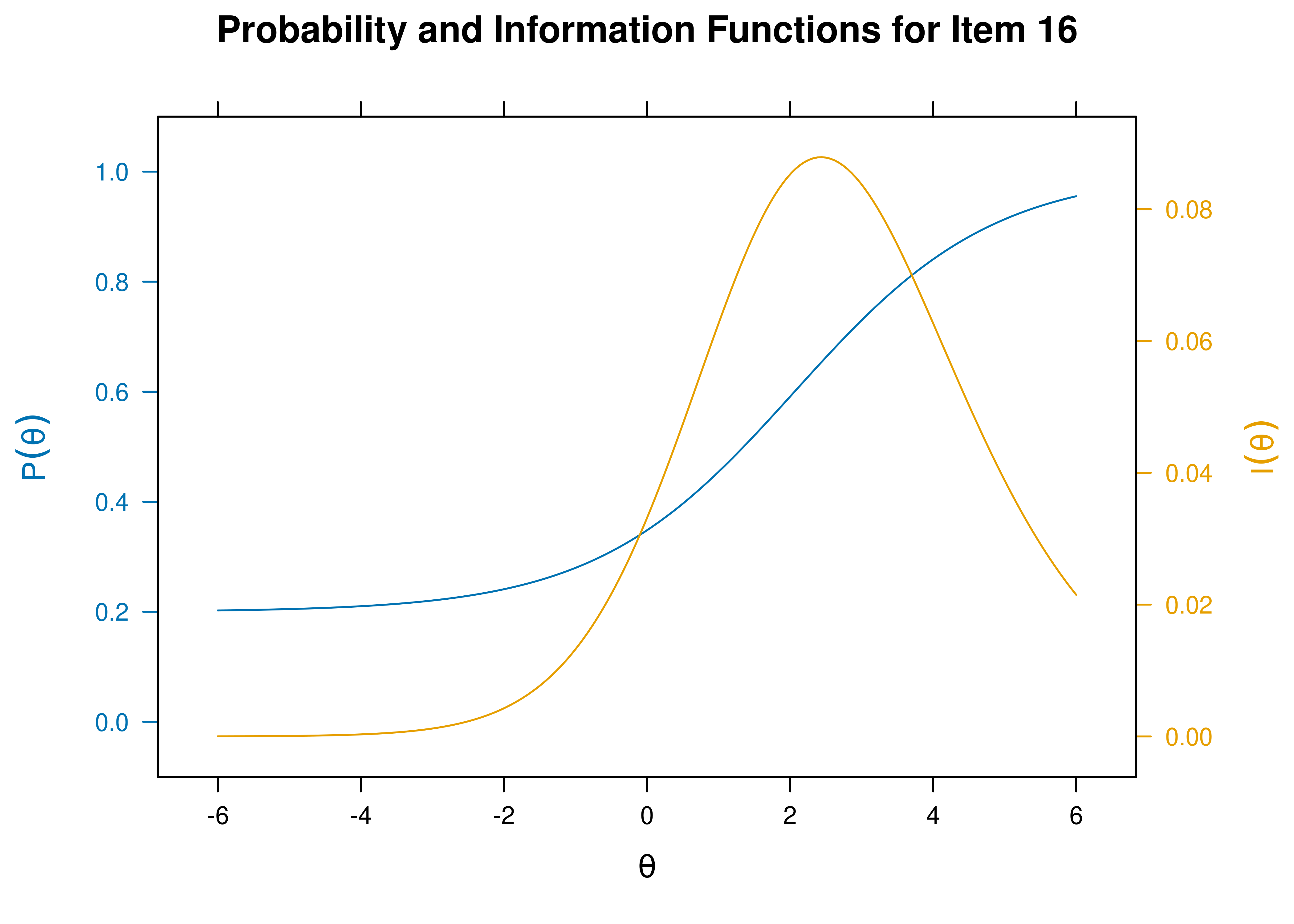
Figure 21.8: Item Characteristic Curves and Information Curves: Item 16.
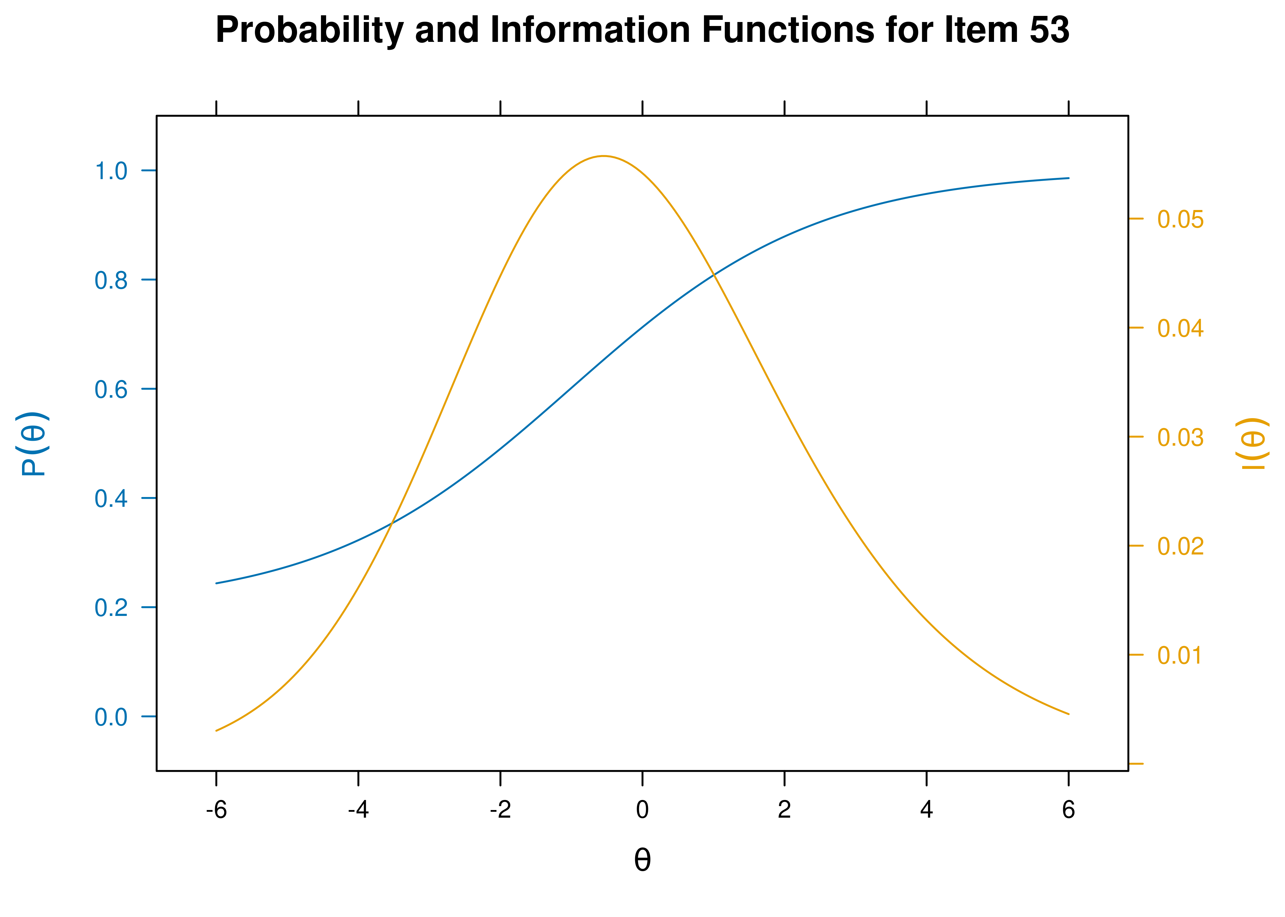
Figure 21.9: Item Characteristic Curves and Information Curves: Item 53.
21.4.6 Create Math Items
Code
questions <- answers <- character(nitems)
choices <- matrix("a", nitems, 5)
spacing <- floor(d - min(d)) + 1 #easier items have more variation

for(i in 1:nitems){
  n1 <- sample(1:100, 1)
  n2 <- sample(101:200, 1)
  ans <- n1 + n2
  questions[i] <- paste(n1, " + ", n2, " = ?", sep = "")
  answers[i] <- as.character(ans)
  ch <- ans + sample(c(-5:-1, 1:5) * spacing[i,], 5)
  ch[sample(1:5, 1)] <- ans
  choices[i,] <- as.character(ch)
}

df <- data.frame(
  Questions = questions,
  Answer = answers,
  Option = choices,
  Type = "radio")
21.4.7 Run Computerized Adaptive Test (CAT)
Set the minimum standard error of measurement for the latent trait (theta; \(\theta\)) that must be reached before stopping the CAT. You can lengthen the CAT by lowering the minimum standard error of measurement, or you can shorten the CAT by raising the minimum standard error of measurement.
Run the CAT and stop once the standard error of measurement for the latent trait (theta; \(\theta\)) becomes \(0.3\) or lower.
Code
21.4.8 CAT Results
 n.items.answered  Theta_1 SE.Theta_1
27 0.238911 0.2975387$final_estimates
Theta_1
Estimates 0.2389110
SEs 0.2975387
$raw_responses
[1] "230" "170" "167" "177" "175" "216" "177" "218" "184" "191" "184" "202"
[13] "294" "204" "200" "204" "264" "242" "177" "189" "267" "200" "235" "149"
[25] "248" "180" "239"
$scored_responses
[1] 1 1 1 1 0 1 0 1 1 1 0 1 0 1 0 1 0 1 0 1 1 0 1 0 1 1 1
$items_answered
[1] 70 54 92 19 43 23 97 30 1 41 40 31 89 5 66 96 48 79 7 88 75 59 13 26 71
[26] 81 29
$thetas_history
Theta_1
[1,] 0.0000000
[2,] 0.4056545
[3,] 0.7815060
[4,] 0.9750919
[5,] 1.1561966
[6,] 0.7421218
[7,] 0.8464452
[8,] 0.5304194
[9,] 0.6256858
[10,] 0.7128811
[11,] 0.7809691
[12,] 0.6338431
[13,] 0.6792420
[14,] 0.5228702
[15,] 0.5589624
[16,] 0.3679772
[17,] 0.4110162
[18,] 0.3112852
[19,] 0.3505818
[20,] 0.1782808
[21,] 0.2190867
[22,] 0.2576467
[23,] 0.1698955
[24,] 0.2023291
[25,] 0.1355895
[26,] 0.1602090
[27,] 0.1960021
[28,] 0.2389110
$thetas_SE_history
Theta_1
[1,] 1.0000000
[2,] 0.9069127
[3,] 0.8093285
[4,] 0.7266039
[5,] 0.6878798
[6,] 0.6098350
[7,] 0.5592082
[8,] 0.5192925
[9,] 0.4820574
[10,] 0.4630971
[11,] 0.4487481
[12,] 0.4224150
[13,] 0.4079867
[14,] 0.3918681
[15,] 0.3778294
[16,] 0.3693179
[17,] 0.3568027
[18,] 0.3507425
[19,] 0.3408871
[20,] 0.3437896
[21,] 0.3332037
[22,] 0.3252183
[23,] 0.3240032
[24,] 0.3164469
[25,] 0.3147717
[26,] 0.3076080
[27,] 0.3017742
[28,] 0.2975387
$terminated_sucessfully
[1] TRUE21.4.8.1 CAT Standard Errors
Standard errors of measurement of a person’s estimated construct level (theta; \(\theta\)) as a function of the item (presented in the order that items were administered as part of the CAT) are in Figure 21.10.
Initially, the respondent got the first items correct, which raised the estimate of their construct level. However, as the respondent got more items incorrect, the CAT converged upon the estimate that the person has a construct level around \(theta = 0.24\), which means that the person scored slightly above average (i.e., 0.24 standard deviations above the mean).
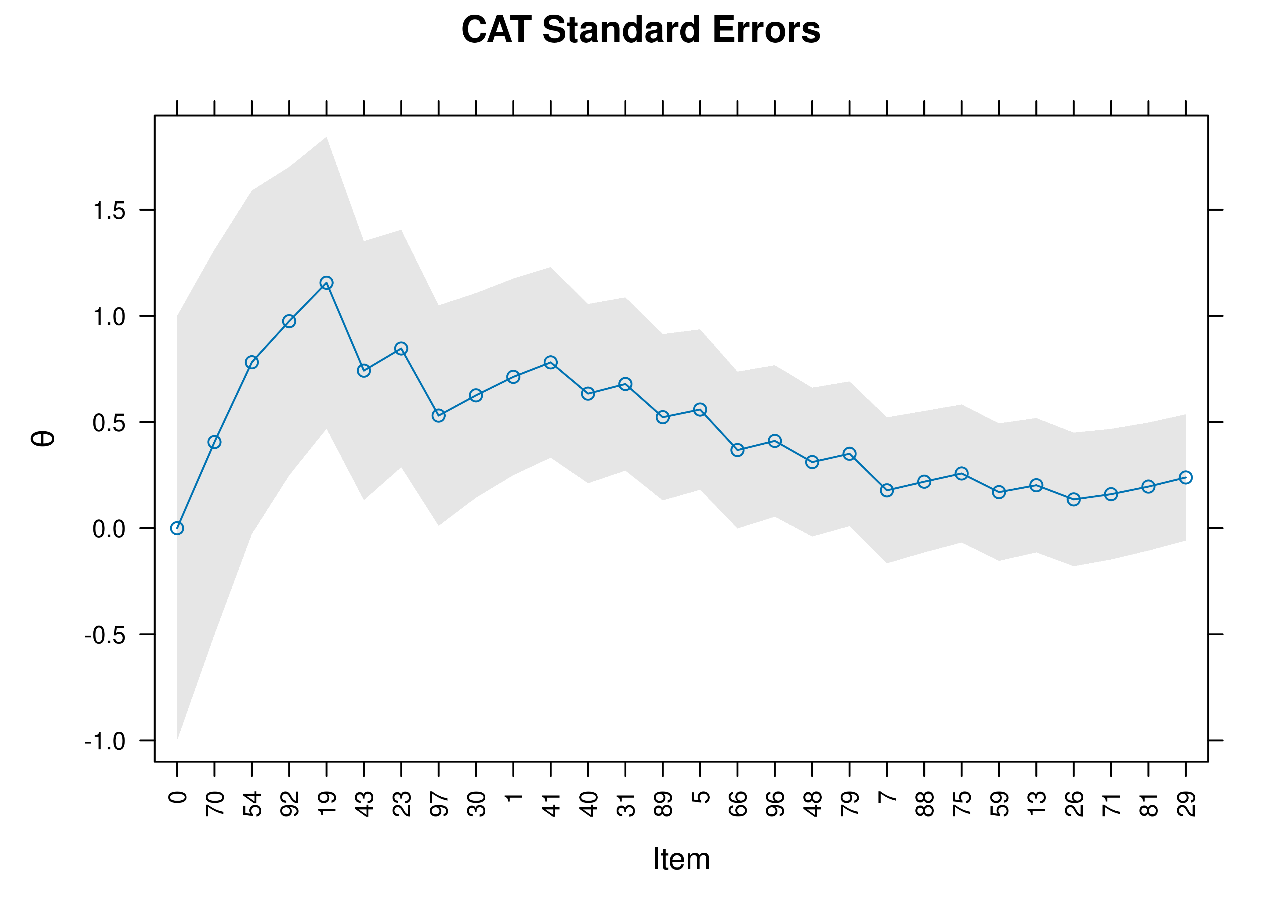
Figure 21.10: Standard Errors of Measurement Around Theta in a Computerized Adaptive Test.
21.4.8.2 CAT 95% Confidence Interval
95% confidence intervals of a person’s estimated construct level (theta; \(\theta\)) as a function of the item (presented in the order that items were administered as part of the CAT) are in Figure 21.11.
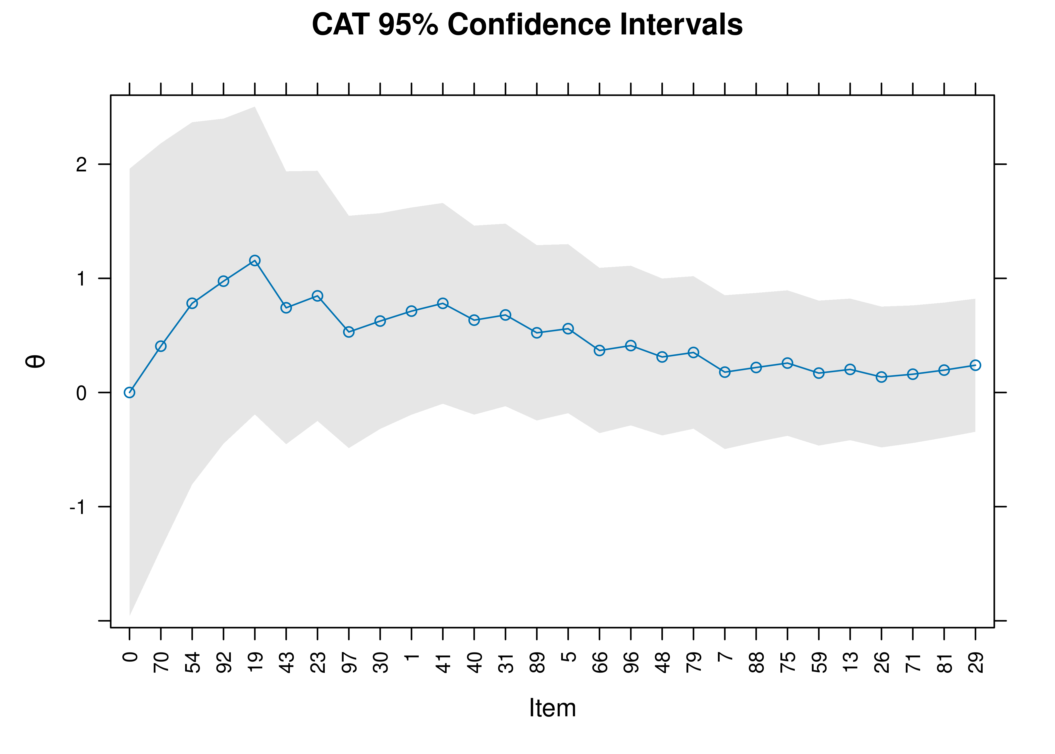
Figure 21.11: 95% Confidence Interval of Theta in a Computerized Adaptive Test.
21.5 Creating a Computerized Adaptive Test From an Item Response Theory Model
You can create a computerized adaptive test from any item response theory model.
21.5.1 Create Items
For instance, below we create a matrix with the questions and response options from the graded response model that we fit in Section 8.9 in Chapter 8 on item response theory.
Code
[1] "Comfort" "Work" "Future" "Benefit"Code
questionsGRM <- c(
  "Science and technology are making our lives healthier, easier and more comfortable.",
  "The application of science and new technology will make work more interesting.",
  "Thanks to science and technology, there will be more opportunities for the future generations.",
  "The benefits of science are greater than any harmful effect it may have."
)

responseOptionsGRM <- c(
  "strongly disagree",
  "disagree to some extent",
  "agree to some extent",
  "strongly agree"
)

numResponseOptionsGRM <- length(responseOptionsGRM)

choicesGRM <- matrix("a", numItemsGRM, numResponseOptionsGRM)

for(i in 1:numItemsGRM){
  choicesGRM[i,] <- responseOptionsGRM
}

dfGRM <- data.frame(
  Questions = questionsGRM,
  Option = choicesGRM,
Type = "radio")21.6 Conclusion
Computer-administered and online assessments have the potential to be both desirable and dangerous. They have key advantages; at the same time, they have both validity and ethical challenges. Best practices for computer-administered and online assessments are provided. Adaptive testing involves having the respondent complete only those items that are needed to answer an assessment question, which can save immense time without sacrificing validity (if done well). There are many approaches to adaptive testing, including manual administration—such as skip rules, basal and ceiling criteria, and the countdown approach—and computerized adaptive testing (CAT) using item response theory. A CAT is designed to locate a person’s level on the construct with as few items as possible. A CAT administers the items that will provide the most information based on participants’ previous responses. CAT typically results in the greatest item savings—around 50% item savings or more.