I need your help!

I want your feedback to make the book better for you and other readers. If you find typos, errors, or places where the text may be improved, please let me know. The best ways to provide feedback are by GitHub or hypothes.is annotations.

Opening an issue or submitting a pull request on GitHub: https://github.com/isaactpetersen/Principles-Psychological-Assessment

Adding an annotation using hypothes.is. To add an annotation, select some text and then click the symbol on the pop-up menu. To see the annotations of others, click the symbol in the upper right-hand corner of the page.

Chapter 2 Scores and Scales

Assessments yield information. The information is encoded in scores or in other types of data. It is important to consider the different types of data because the types of data restrict what options are available to analyze the data.

2.1 Getting Started

2.1.1 Load Libraries

First, we load the R packages used for this chapter:

Code

library("petersenlab") #to install: install.packages("remotes"); remotes::install_github("DevPsyLab/petersenlab")
library("dplyr")
library("tidyverse")
library("tinytex")
library("knitr")
library("rmarkdown")
library("bookdown")

2.1.2 Prepare Data

2.1.2.1 Simulate Data

For this example, we simulate data below. For reproducibility, we set the seed below. Using the same seed will yield the same answer every time. There is nothing special about this particular seed.

Code

set.seed(52242)

rawData <- rnorm(
  n = 1000,
  mean = 200,
  sd = 30)

scores <- data.frame(
  rawData = rawData,
  rawDataNoMissing = rawData)

2.1.2.2 Add Missing Data

Adding missing data to dataframes helps make examples more realistic to real-life data and helps you get in the habit of programming to account for missing data.

Code

scores$rawData[c(5,10)] <- NA

2.2 Data Types

There are four general data types: nominal, ordinal, interval, and ratio. Depending on the use of the variable, the data could fall into more than one category. The type of data influences what kinds of data analysis you can do. For instance, parametric statistical analysis (e.g., t test, analysis of variance [ANOVA], and linear regression) assumes that data are interval or ratio.

2.2.1 Nominal

Nominal data are distinct categories. They are categorical and unordered. Nominal data make no quantitative claims. Nominal data represent things that we can name (e.g., cat and dog). Nominal data can be represented with numbers. For example, zip codes are nominal. Numbers that represent a participant’s sex, race, or ethnicity are also nominal. Categorical data are often dummy-coded into binary (i.e., dichotomous) variables, which represent nominal data. Higher numbers of nominal data do not reflect higher (or lower) levels of the construct because the numbers represent categories that do not have an order.

2.2.2 Ordinal

Ordinal data are ordered categories: they have a name and an order. They make no claim about the conceptual distance between the ranks, only that higher values represent higher (or lower) levels of the construct. For example, ranks following a race are ordinal—that is, the person with rank 1 finished before the person with rank 2, who finished before the person with rank 3 (1 > 2 > 3 > 4). Ordinal data make a limited claim because the conceptual distance between adjacent numbers is not the same. For instance, the person who finished the race first might have finished 10 minutes before the second-place finisher; whereas the third-place finisher might have finished 1 second after the second-place finisher.

That is, just because the numbers have the same mathematical distance does not mean that they represent the same conceptual distance on the construct. For example, if the respondent is asked how many drinks they had in the past day, and the options are 0 = 0 drinks; 1 = 1–2 drinks; 2 = 3 or more drinks, the scale is ordinal. Even though the numbers have the same mathematical distance (1, 2, 3), they do not represent the same conceptual distance. Most data in psychology are ordinal data even though they are often treated as if they were interval data.

2.2.3 Interval

Interval data are ordered and have meaningful distances (i.e., equal spacing between intervals). You can sum interval data (e.g., 2 is 2 away from 4), but you cannot multiply interval data (\(2 \times 2 \ne 4\)). Examples of interval data are temperatures in Fahrenheit and Celsius—100 degrees Fahrenheit is not twice as hot as 50 degrees Fahrenheit. A person’s number of years of education is interval, whereas educational attainment (e.g., high school degree, college degree, graduate degree) is only ordinal. Although much data in psychology involve numbers that have the same mathematical distance between intervals, the intervals likely do not represent the same conceptual distance. For example, the difference in severity of two people who have two symptoms and four symptoms of depression, respectively, may not be the same difference in depression severity as two people who have four symptoms and six symptoms, respectively.

2.2.4 Ratio

Ratio data are ordered, have meaningful distances, and have a true (absolute) zero that represents absence of the construct. With ratio data, multiplicative relationships are true. An example of ratio data is temperature in Kelvin—100 degrees Kelvin is twice as hot as 50 degrees Kelvin. There is a dream of having ratio scales in psychology, but we still do not have a true zero with psychological constructs—what does total absence of depression mean (apart from a dead person)?

2.3 Score Transformation

There are a number of score transformations, depending on the goal. Some score transformations (e.g., log transform) seek to make data more normally distributed to meet assumptions of particular analysis approaches. Score transformations alter the original (raw) data. If you change the data, it can change the results. Score transformations are not neutral.

2.3.1 Raw Scores

Raw scores are the original data, or they may be aggregations (e.g., sums or means) of multiple items. Raw scores are the purest because they are closest to the original operation (e.g., behavior). A disadvantage of raw scores is that they are scale dependent, and therefore they may not be comparable across different measures with different scales. An example histogram of raw scores is in Figure 2.1.

Code

hist(scores$rawData,
     xlab = "Raw Scores",
     main = "Histogram of Raw Scores")

Figure 2.1: Histogram of Raw Scores.

2.3.2 Norm-Referenced Scores

Norm-referenced scores are scores that are referenced to some norm. A norm is a standard of comparison. For instance, you may be interested in how well a participant performed relative to other children of the same sex, age, grade, or ethnicity. However, interpretation of norm-referenced scores depends on the measure and on the normative sample. A person’s norm-referenced score can vary widely depending on which norms are used. Which reference group should you use? Age? Sex? Age and sex? Grade? Ethnicity? The optimal reference group depends on the purpose of the assessment. The quality of the norms also depends on the representativeness of the reference group compared to the population of interest. Pros and cons of group-based norms are discussed in Section 16.5.2.2.2.

A standard normal distribution on various norm-referenced scales is depicted in Figure 2.2, as adapted from Bandalos (2018).

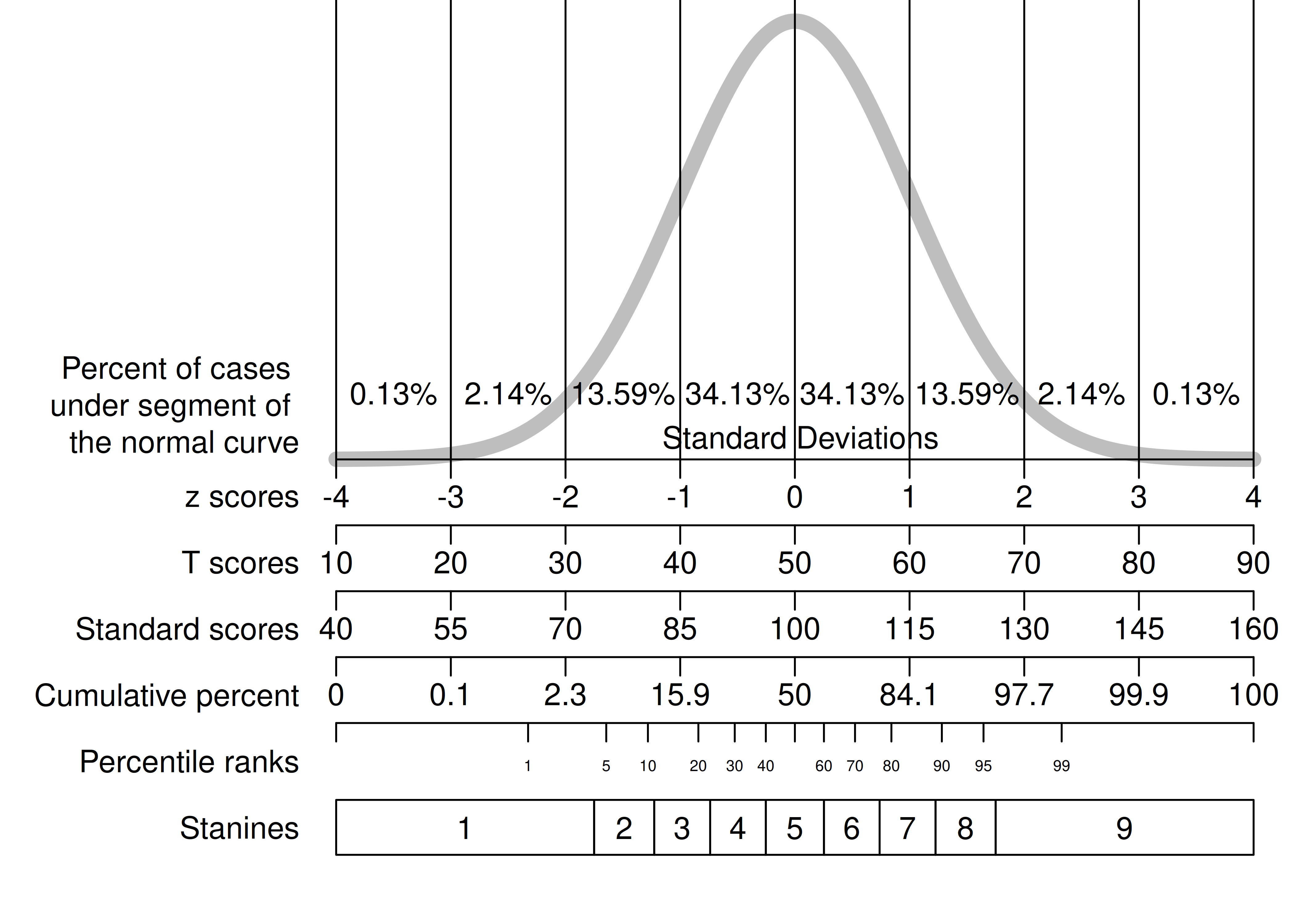
Figure 2.2: Various Norm-Referenced Scales.

2.3.2.1 Percentile Ranks

A percentile rank reflects what percent of people a person scored higher than, in a given group (i.e., norm). Percentile ranks are frequently used for tests of intellectual/cognitive ability, academic achievement, academic aptitude, and grant funding. They seem like interval data, but they are not intervals because the conceptual spacing between the numbers is not equal. The difference in ability for two people who scored at the 99th and 98th percentile, respectively, is not the same as the difference in ability for two people who scored at the 49th and 50th percentile, respectively. Percentile ranks are only judged against a baseline; there is no subtraction.

Percentile ranks have unusual effects. There are lots of people in the middle of a distribution, so a very small difference in raw scores gets expanded out in percentiles. For instance, a raw score of 20 may have a percentile rank of 50, but a raw score of 24 may have a percentile rank of 68. However, a larger raw score change at the ends of the distribution may have a smaller percentile change. For example, a raw score of 120 may have a percentile rank of 97, whereas a raw score of 140 may have a percentile rank of 99. Thus, percentile ranks stretch out differences for some people but constrict differences for others.

Here is an example of how to calculate percentile ranks using the dplyr package from the tidyverse (Wickham et al., 2019; Wickham, 2021):

Code

scores$percentileRank <- 
  percent_rank(scores$rawDataNoMissing) * 100

A histogram of percentile rank scores is in Figure 2.3.

Code

hist(scores$percentileRank,
     xlab = "Percentile Ranks",
     main = "Histogram of Percentile Ranks")

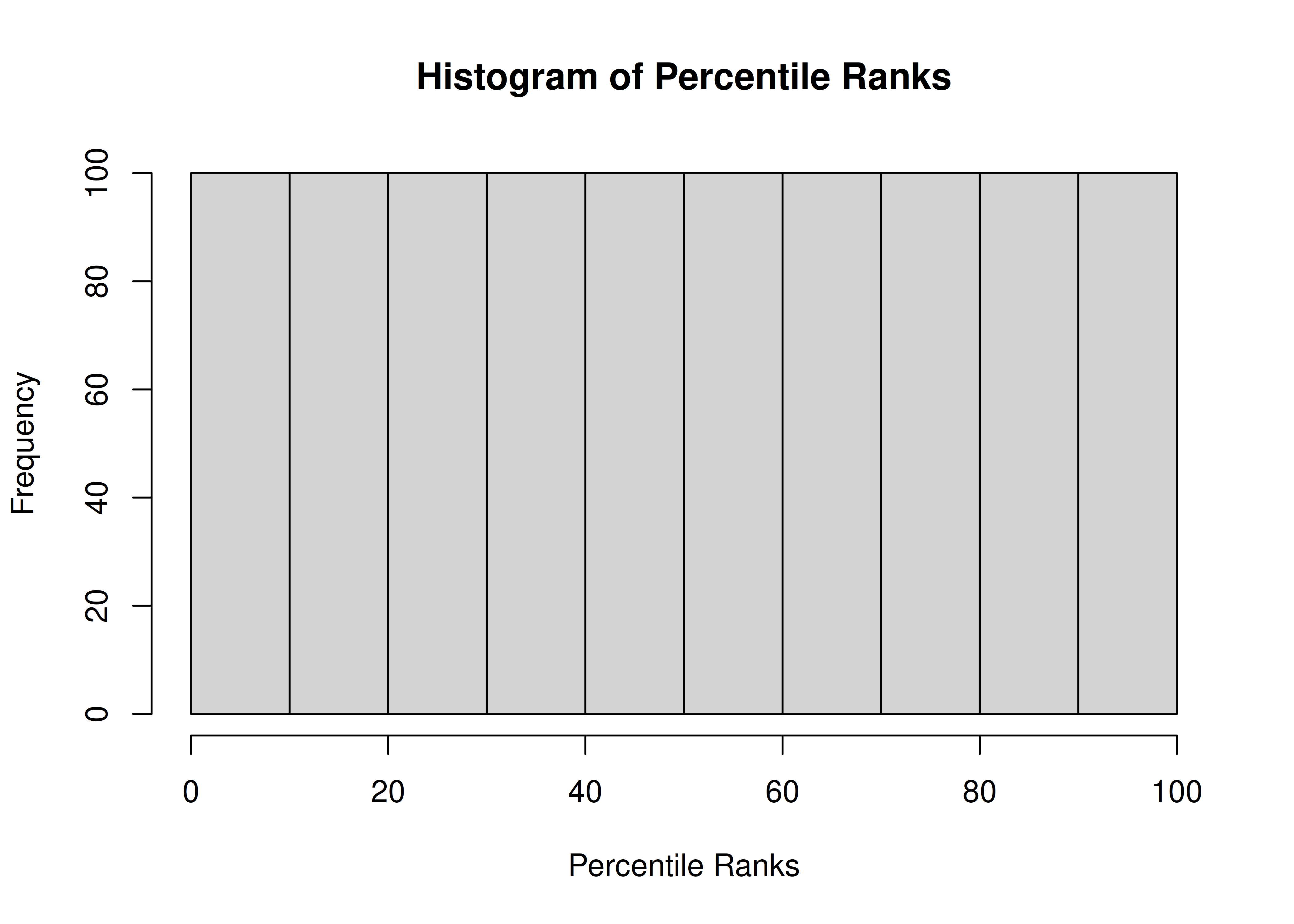
Figure 2.3: Histogram of Percentile Ranks.

2.3.2.2 Deviation (Standardized) Scores

Deviation or standardized scores are the transformation of raw scores to a normal distribution using some norm. The norm could be a comparison group, or it could be the sample itself. With deviation scores, you have similar challenges as with percentile ranks, including which reference group to use, but there are additional challenges. Deviation scores are more informative when the scores are normally distributed compared to when the scores are skewed. If scores are skewed, it can lead to two z scores on the opposite side of the mean having different probabilities.

Many constructs we study in psychology are not normally distributed. For example, the frequency of hallucinations among people would show a positively skewed distribution with a truncation at zero, representing a floor effect—i.e., most people do not show hallucinations. For instance, consider a hypothetical distribution of hallucinations. It might follow a folded distribution, as depicted in Figure 2.4:

Code

hist(rbinom(100000, 300, .01),
     breaks = 8,
     xlab = "Hallucinations (Raw Score)",
     main = "Histogram of Hallucinations (Raw Score)")

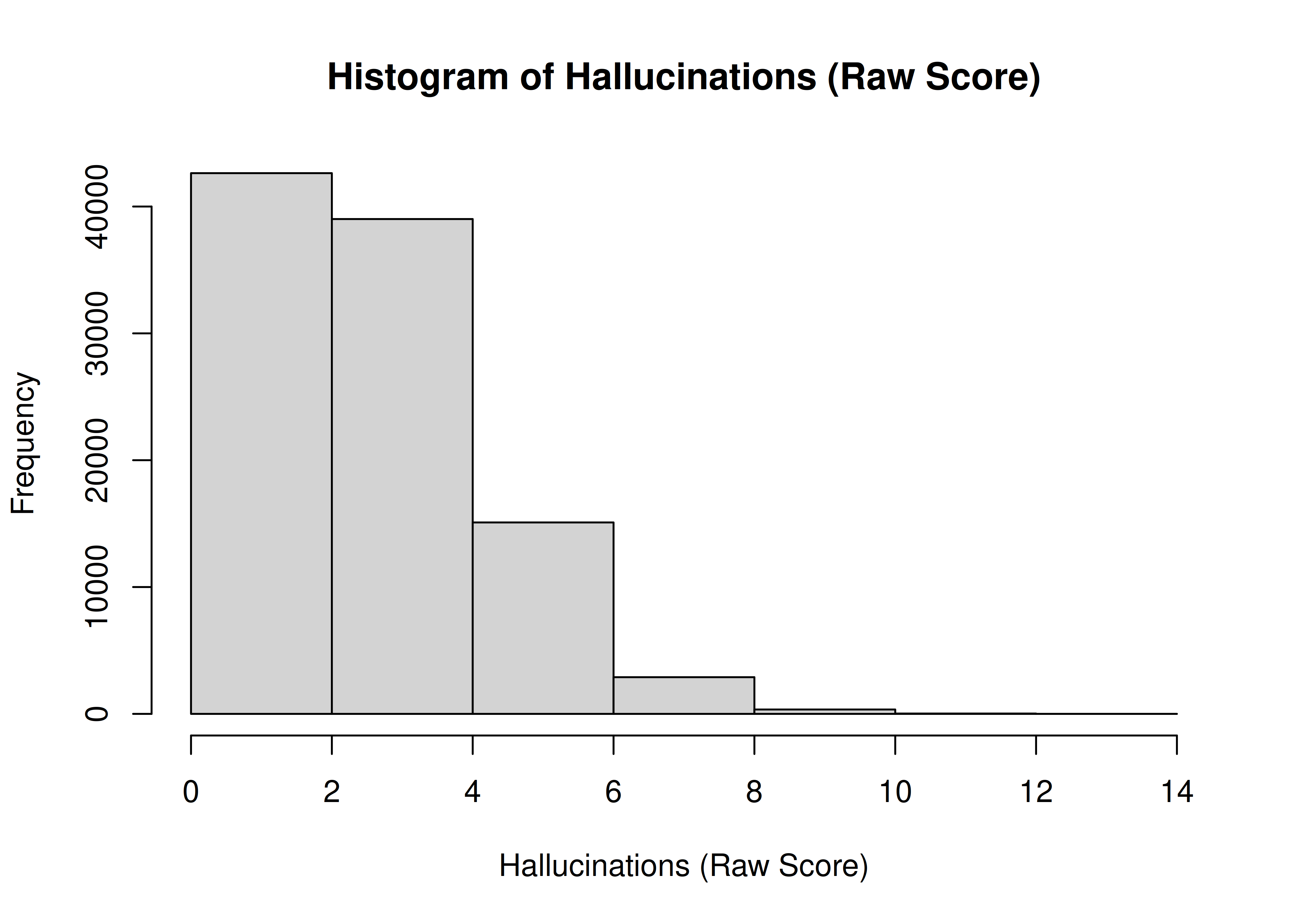
Figure 2.4: Histogram of Hallucinations (Raw Score).

Now consider the same distribution converted to a standardized (z) score, as depicted in Figure 2.5:

Code

hist(scale(rbinom(100000, 300, .01)),
     breaks = 8,
     xlab = "Hallucinations (z Score)",
     main = "Histogram of Hallucinations (z Score)")

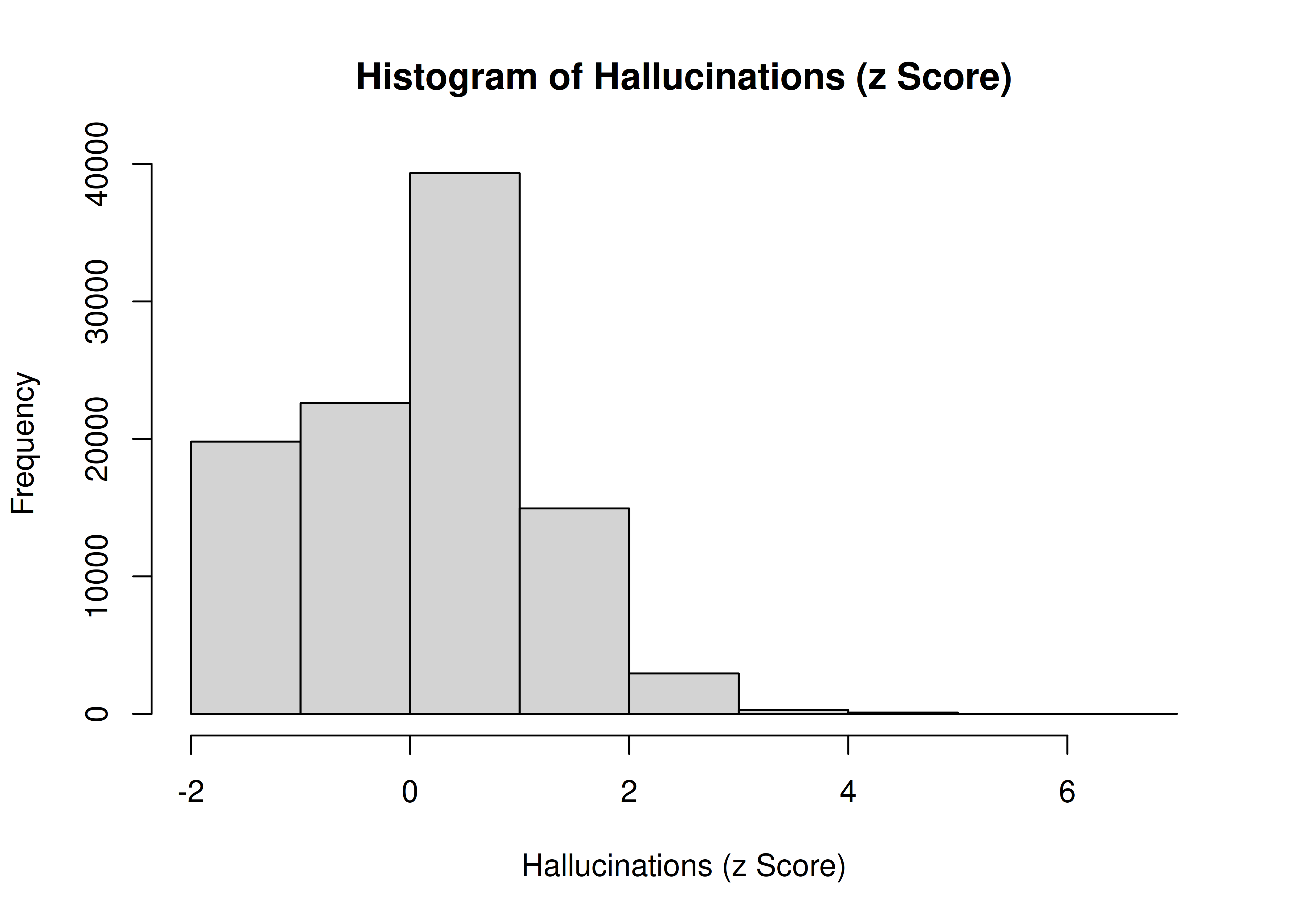
Figure 2.5: Histogram of Hallucinations (z Score).

Thus, you can compute a deviation score, but it may not be meaningful if the data and underlying construct are not normally distributed.

2.3.2.2.1 z scores

The z score is the most common standardized score, and it can help put scores from different measures with different scales onto the same playing field. z scores have a mean of zero and a standard deviation of one. To get a z score that uses the sample as its own norm, subtract the mean from all scores and divide by the standard deviation. Every z score represents how far that person’s score is from the (normed) average, represented in standard deviation units. With a standard normal curve, 68% of scores fall within one standard deviation of the mean. 95% of scores fall within two standard deviations of the mean. 99.7% of scores fall within three standard deviations of the mean.

The area under a normal curve within one standard deviation of the mean is calculated below using the pnorm() function, which calculates the cumulative density function for a normal curve.

Code

stdDeviations <- 1

pnorm(stdDeviations) - pnorm(stdDeviations * -1)

[1] 0.6826895

The area under a normal curve within one standard deviation of the mean is depicted in Figure 2.6.

Code

x <- seq(-4, 4, length = 200)
y <- dnorm(x, mean = 0, sd = 1)
plot(x, y, type = "l",
     xlab = "z Score",
     ylab = "Normal Density")

x <- seq(stdDeviations * -1, stdDeviations, length = 100)
y <- dnorm(x, mean = 0, sd = 1)
polygon(c(stdDeviations * -1, x, stdDeviations),
        c(0, y, 0),
        col = "blue")

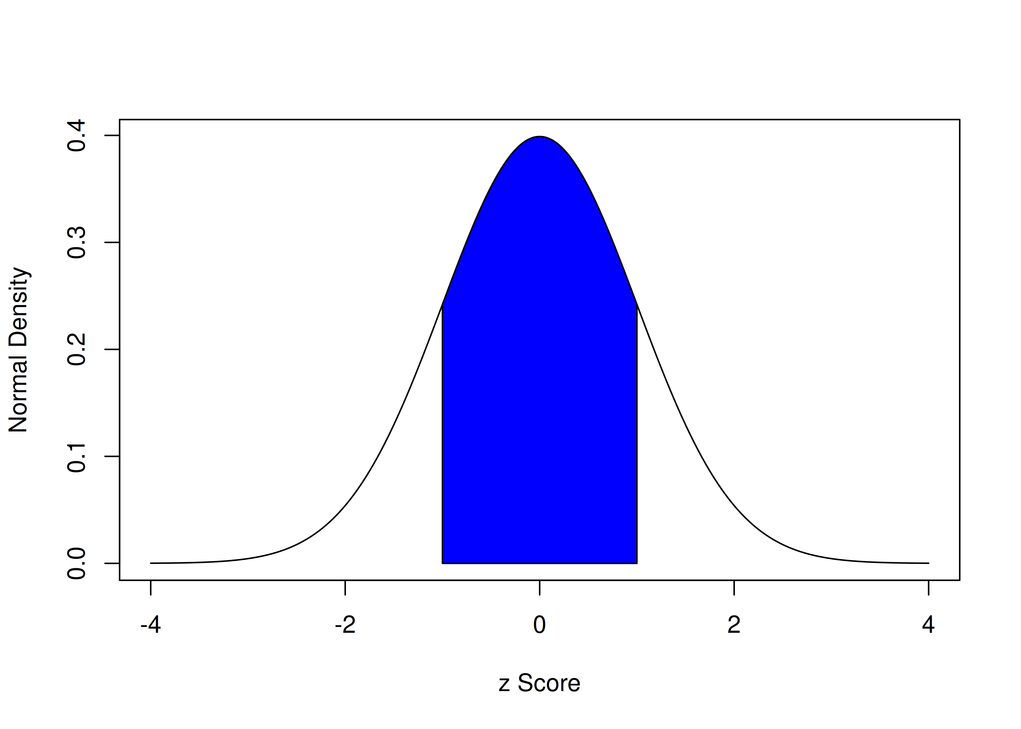
Figure 2.6: Density of Standard Normal Distribution. The blue region represents the area within one standard deviation of the mean.

The area under a normal curve within two standard deviations of the mean is calculated below:

Code

stdDeviations <- 2

pnorm(stdDeviations) - pnorm(stdDeviations * -1)

[1] 0.9544997

The area under a normal curve within two standard deviations of the mean is depicted in Figure 2.7.

Code

x <- seq(-4, 4, length = 200)
y <- dnorm(x, mean = 0, sd = 1)
plot(x, y, type = "l",
     xlab = "z Score",
     ylab = "Normal Density")

x <- seq(stdDeviations * -1, stdDeviations, length = 100)
y <- dnorm(x, mean = 0, sd = 1)
polygon(c(stdDeviations * -1, x, stdDeviations),
        c(0, y, 0),
        col = "blue")

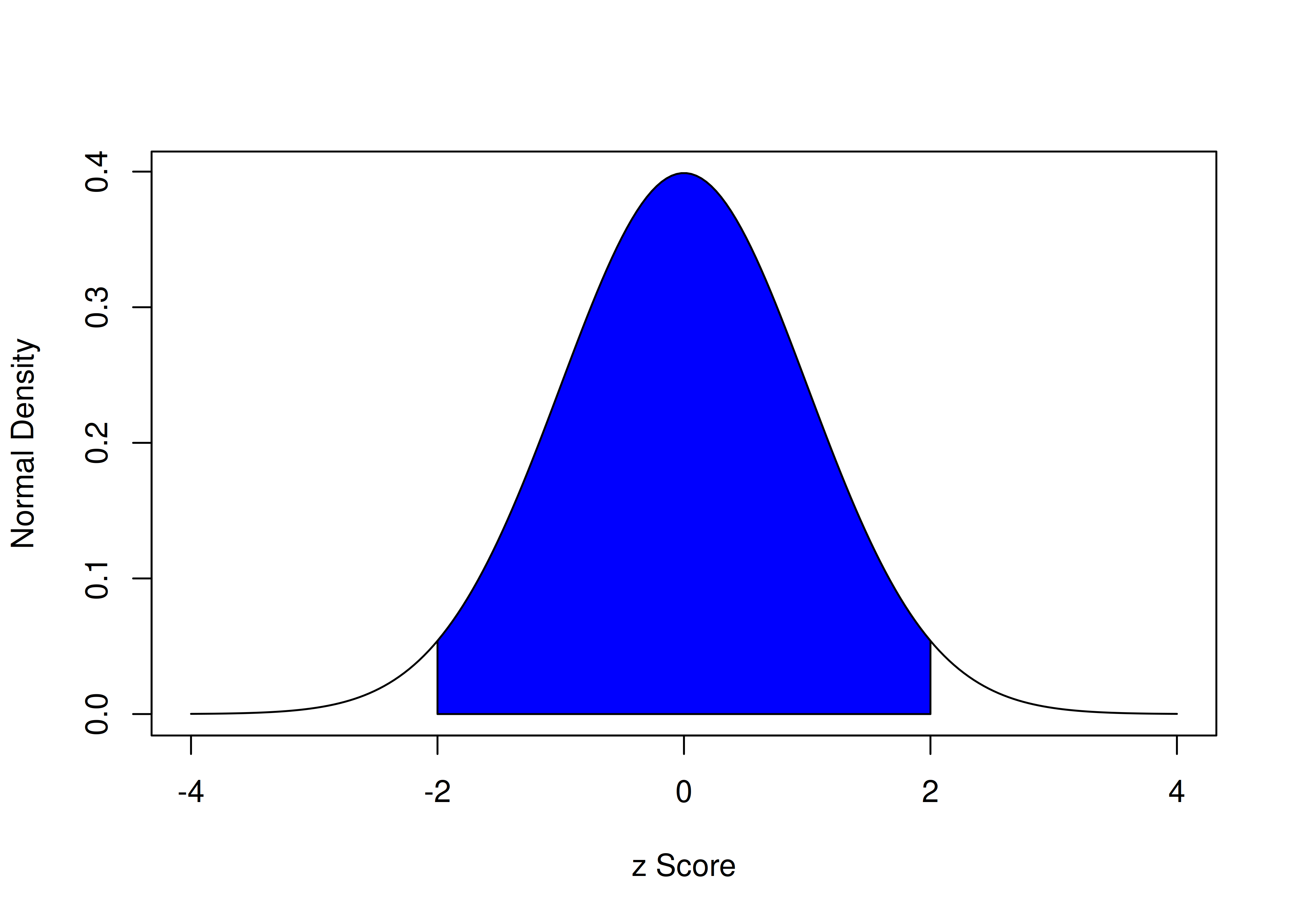
Figure 2.7: Density of Standard Normal Distribution. The blue region represents the area within two standard deviations of the mean.

The area under a normal curve within three standard deviations of the mean is calculated below:

Code

stdDeviations <- 3

pnorm(stdDeviations) - pnorm(stdDeviations * -1)

[1] 0.9973002

The area under a normal curve within three standard deviations of the mean is depicted in Figure 2.8.

Code

x <- seq(-4, 4, length = 200)
y <- dnorm(x, mean = 0, sd = 1)
plot(x, y, type = "l",
     xlab = "z Score",
     ylab = "Normal Density")

x <- seq(stdDeviations * -1, stdDeviations, length = 100)
y <- dnorm(x, mean = 0, sd = 1)
polygon(c(stdDeviations * -1, x, stdDeviations),
        c(0, y, 0),
        col = "blue")

Figure 2.8: Density of Standard Normal Distribution. The blue region represents the area within three standard deviations of the mean.

Alternatively, if you want to determine the z score associated with a particular percentile in a normal distribution, you can use the qnorm() function.

For instance, the z score associated with the 37th percentile is:

Code

qnorm(.37)

[1] -0.3318533

z scores are calculated using Equation (2.1):

\[\begin{equation} z = \frac{x - \mu}{\sigma} \tag{2.1} \end{equation}\]

where \(x\) is the observed score, \(\mu\) is the mean observed score, and \(\sigma\) is the standard deviation of observed scores.

Code

scores$zScore <- scale(scores$rawData)

all.equal(
  as.vector(scores$zScore),
  (scores$rawData - mean(scores$rawData, na.rm = TRUE)) / 
    sd(scores$rawData, na.rm = TRUE))

[1] TRUE

An example histogram of z scores is in Figure 2.9.

Code

hist(scores$zScore,
     xlab = "z Scores",
     main = "Histogram of z Scores")

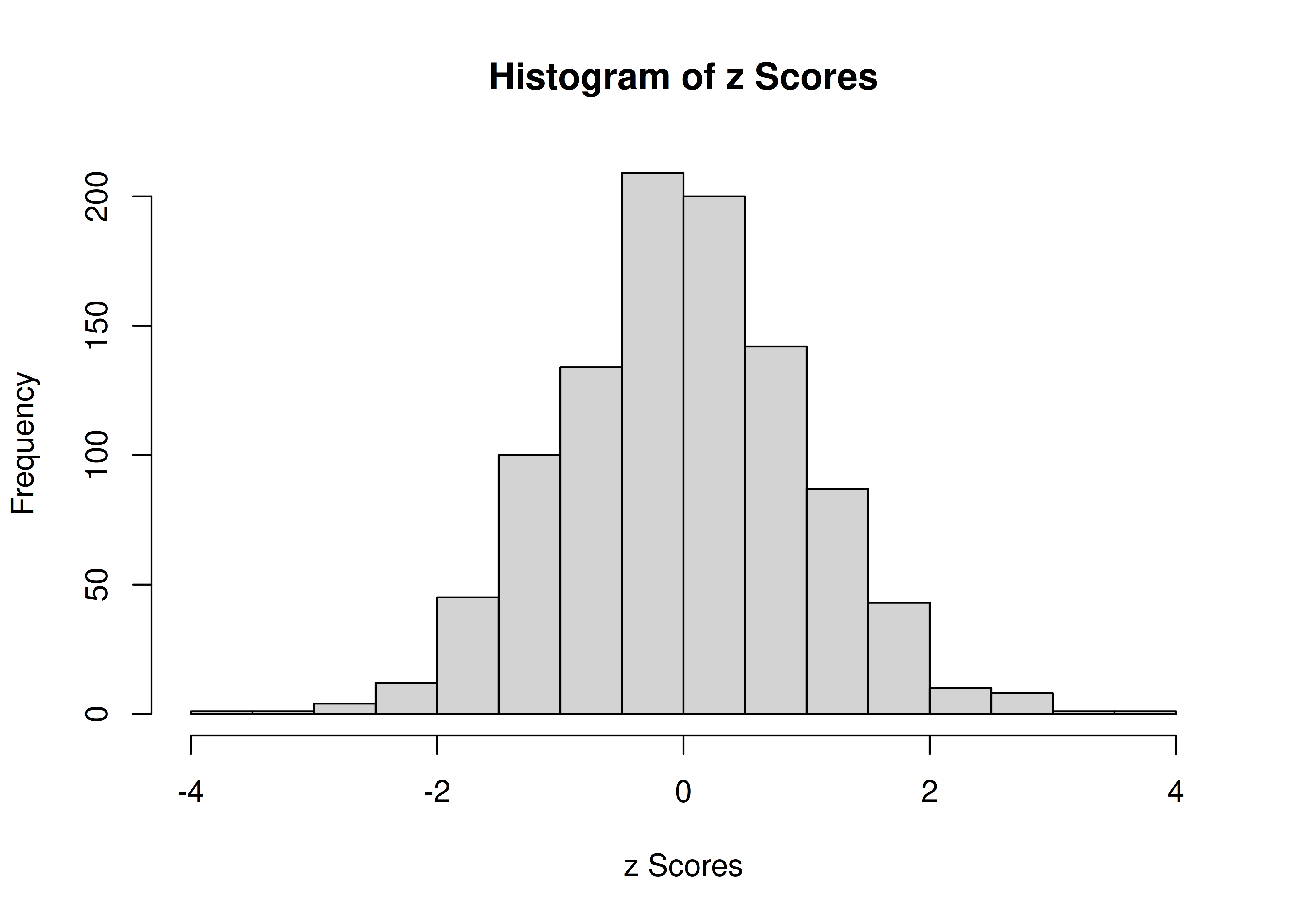
Figure 2.9: Histogram of z Scores.

2.3.2.2.2 T scores

T scores have a mean of 50 and a standard deviation of 10. T scores are frequently used with personality and symptom measures, where clinical cutoffs are often set at 70 (i.e., two standard deviations above the mean). For the Minnesota Multiphasic Personality Inventory (MMPI), you would examine peaks (elevations \(\ge\) 70) and absences (\(\le\) 30).

T scores are calculated using Equation (2.2):

\[\begin{equation} T = 50 + 10z \tag{2.2} \end{equation}\]

where \(z\) are z scores.

Code

scores$tScore <- 50 + 10*scale(scores$rawData)

An example histogram of T scores is in Figure 2.10.

Code

hist(scores$tScore,
     xlab = "T Scores",
     main = "Histogram of T Scores")

Figure 2.10: Histogram of T Scores.

2.3.2.2.3 Standard scores

Standard scores have a mean of 100 and a standard deviation of 15. Standard scores are frequently used for tests of intellectual ability, academic achievement, and cognitive ability. Intellectual disability is generally considered an I.Q. standard score less than 70 (two standard deviations below the mean), whereas giftedness is at 130 (two standard deviations above the mean).

Standard scores with a mean of 100 and standard deviation of 15 are calculated using Equation (2.3):

\[\begin{equation} \text{standard score} = 100 + 15z \tag{2.3} \end{equation}\]

where \(z\) are z scores.

Code

scores$standardScore <- 100 + 15*scale(scores$rawData)

An example histogram of standard scores is in Figure 2.11.

Code

hist(scores$standardScore,
     xlab = "Standard Scores",
     main = "Histogram of Standard Scores")

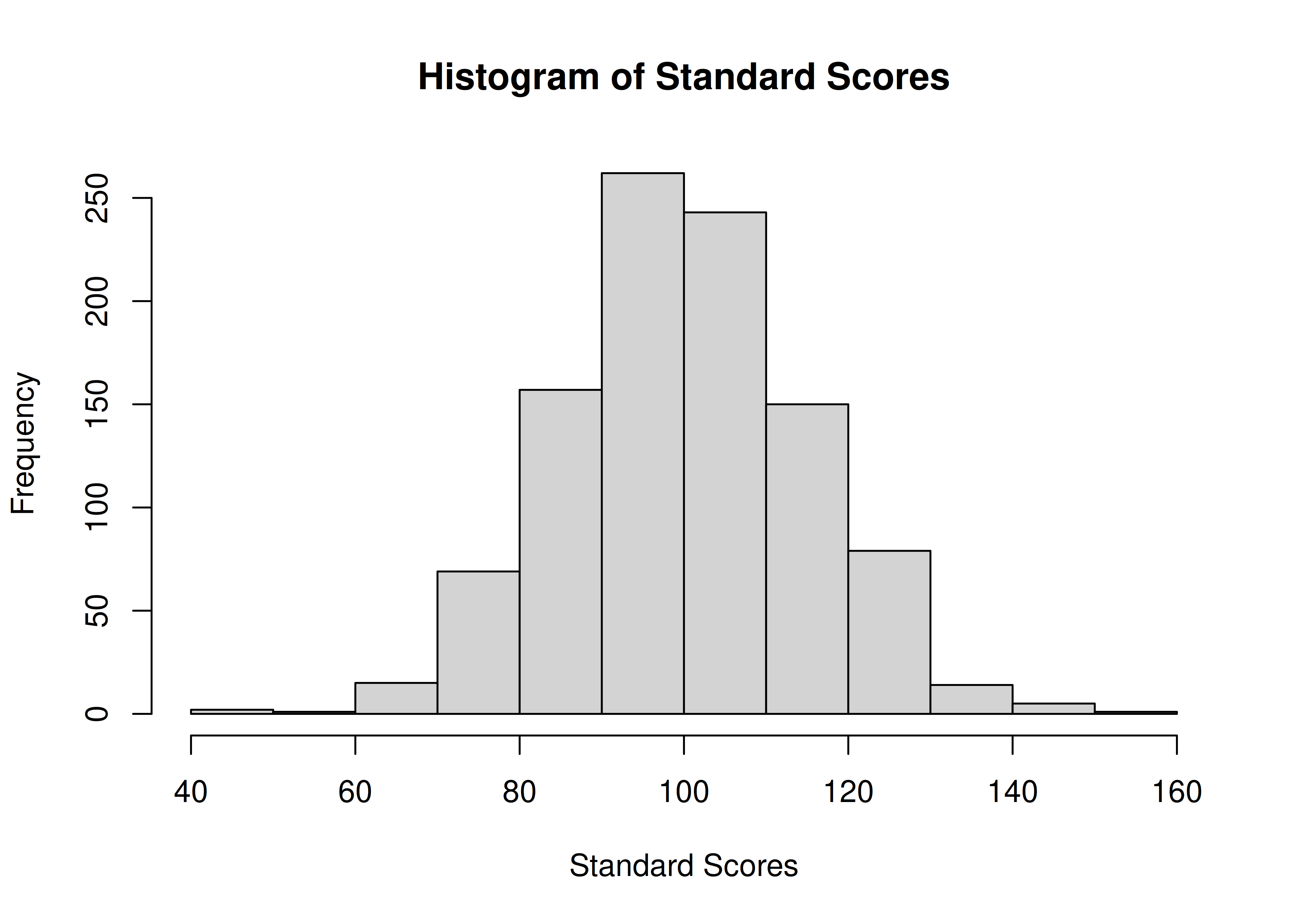
Figure 2.11: Histogram of Standard Scores.

2.3.2.2.4 Scaled scores

Scaled scores are raw scores that have been converted to a standardized metric. The particular metric of the scaled score depends on the measure. On tests of intellectual or cognitive ability, scaled scores commonly have a mean of 10 and a standard deviation of 3.

Using this metric, scaled scores can be calculated using Equation (2.4):

\[\begin{equation} \text{scale score} = 10 + 3z \tag{2.4} \end{equation}\]

where \(z\) are z scores.

Code

scores$scaledScore <- 10 + 3*scale(scores$rawData)

An example histogram of scaled scores is in Figure 2.12.

Code

hist(scores$scaledScore,
     xlab = "Scale Scores",
     main = "Histogram of Scaled Scores")

Figure 2.12: Histogram of Scaled Scores.

2.3.2.2.5 Stanine scores

Stanine scores (short for STANdard Nine) have a mean of 5 and a standard deviation of 2. The scores range from 1–9. Stanine scores are calculated using the bracketed proportions in Table 2.1. The lowest 4% receive a stanine score of 1, the next 7% receive a stanine score of 2, etc.

Table 2.1: Calculating Stanine Scores

Stanine	Bracketed Percent	Cumulative Percent	z Score	Standard Score
1	4%	4%	below −1.75	below 74
2	7%	11%	−1.75 to −1.25	74 to 81
3	12%	23%	−1.25 to −0.75	81 to 89
4	17%	40%	−0.75 to −0.25	89 to 96
5	20%	60%	−0.25 to +0.25	96 to 104
6	17%	77%	+0.25 to +0.75	104 to 111
7	12%	89%	+0.75 to +1.25	111 to 119
8	7%	96%	+1.25 to +1.75	119 to 126
9	4%	100%	above +1.75	above 126

Code

scores$stanineScore <- NA
scores$stanineScore[which(scores$percentileRank <= 4)] <- 1
scores$stanineScore[
  which(scores$percentileRank > 4 & scores$percentileRank <= 11)] <- 2
scores$stanineScore[
  which(scores$percentileRank > 11 & scores$percentileRank <= 23)] <- 3
scores$stanineScore[
  which(scores$percentileRank > 23 & scores$percentileRank <= 40)] <- 4
scores$stanineScore[
  which(scores$percentileRank > 40 & scores$percentileRank <= 60)] <- 5
scores$stanineScore[
  which(scores$percentileRank > 60 & scores$percentileRank <= 77)] <- 6
scores$stanineScore[
  which(scores$percentileRank > 77 & scores$percentileRank <= 89)] <- 7
scores$stanineScore[
  which(scores$percentileRank > 89 & scores$percentileRank <= 96)] <- 8
scores$stanineScore[which(scores$percentileRank > 96)] <- 9

A histogram of stanine scores is in Figure 2.13.

Code

hist(scores$stanineScore,
     xlab = "Stanine Scores",
     main = "Histogram of Stanine Scores",
     breaks = seq(from = 0.5, to = 9.5, by = 1),
     xlim = c(0,10),
     xaxp = c(1,9,8))

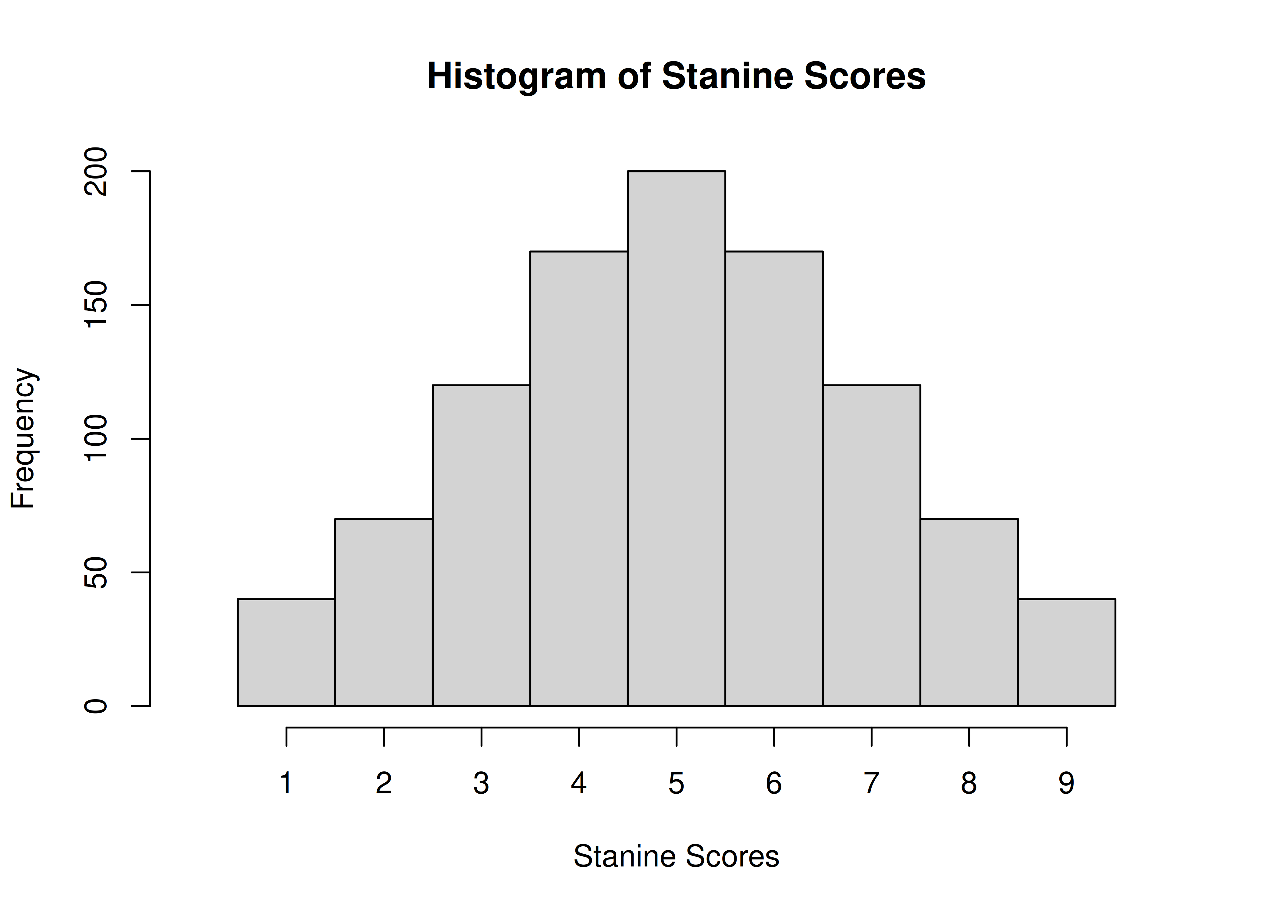
Figure 2.13: Histogram of Stanine Scores.

2.4 Conclusion

It is important to consider the types of data your data are because the types of data restrict what options are available to analyze the data. It is also important to consider whether the data were transformed because score transformations are not neutral—they can impact the results.

2.5 Suggested Readings

Childs et al. (2021): https://dzchilds.github.io/stats-for-bio/data-transformations.html (archived at https://perma.cc/3YEB-QW2V)

2.6 Exercises

References

Bandalos, D. L. (2018). Measurement theory and applications for the social sciences. Guilford Publications.

Childs, D. Z., Hindle, B. J., & Warren, P. H. (2021). APS 240: Data analysis and statistics with R. https://dzchilds.github.io/stats-for-bio/

Wickham, H. (2021). tidyverse: Easily install and load the tidyverse. https://CRAN.R-project.org/package=tidyverse

Wickham, H., Averick, M., Bryan, J., Chang, W., McGowan, L. D., François, R., Grolemund, G., Hayes, A., Henry, L., Hester, J., Kuhn, M., Pedersen, T. L., Miller, E., Bache, S. M., Müller, K., Ooms, J., Robinson, D., Seidel, D. P., Spinu, V., … Yutani, H. (2019). Welcome to the tidyverse. Journal of Open Source Software, 4(43), 1686. https://doi.org/10.21105/joss.01686

Feedback

Please consider providing feedback about this textbook, so that I can make it as helpful as possible. You can provide feedback at the following link: https://forms.gle/95iW4p47cuaphTek6