I want your feedback to make the book better for you and other readers. If you find typos, errors, or places where the text may be improved, please let me know. The best ways to provide feedback are by GitHub or hypothes.is annotations.
Opening an issue or submitting a pull request on GitHub: https://github.com/isaactpetersen/Principles-Psychological-Assessment
Adding an annotation using hypothes.is.
To add an annotation, select some text and then click the
symbol on the pop-up menu.
To see the annotations of others, click the
symbol in the upper right-hand corner of the page.
Chapter 7 Structural Equation Modeling
“All models are wrong, but some are useful.”
— George Box (1979, p. 202)
7.1 Overview of SEM
Structural equation modeling is an advanced modeling approach that allows estimating latent variables to account for measurement error and to get purer estimates of constructs.
7.2 Getting Started
7.2.1 Load Libraries
Code
library("petersenlab") #to install: install.packages("remotes"); remotes::install_github("DevPsyLab/petersenlab")
library("lavaan")
library("semTools")
library("semPlot")
library("simsem")
library("snow")
library("mice")
library("quantreg")
library("nonnest2")
library("MOTE")
library("tidyverse")
library("here")
library("tinytex")
7.2.2 Prepare Data
7.2.2.1 Simulate Data
For reproducibility, I set the seed below. Using the same seed will yield the same answer every time. There is nothing special about this particular seed.
The petersenlab package (Petersen, 2025) includes a complement() function (archived at https://perma.cc/S26F-QSW3) that simulates data with a specified correlation in relation to an existing variable.
PoliticalDemocracy refers to the Industrialization and Political Democracy data set from the lavaan package (Rosseel et al., 2022), and it contains measures of political democracy and industrialization in developing countries.
Code
sampleSize <- 300

set.seed(52242)

v1 <- complement(PoliticalDemocracy$y1, .4)
v2 <- complement(PoliticalDemocracy$y1, .4)
v3 <- complement(PoliticalDemocracy$y1, .4)
v4 <- complement(PoliticalDemocracy$y1, .4)

PoliticalDemocracy$v1 <- v1
PoliticalDemocracy$v2 <- v2
PoliticalDemocracy$v3 <- v3
PoliticalDemocracy$v4 <- v4

measure1 <- rnorm(n = sampleSize, mean = 50, sd = 10)
measure2 <- measure1 + rnorm(n = sampleSize, mean = 0, sd = 15)
measure3 <- measure1 + measure2 + rnorm(n = sampleSize, mean = 0, sd = 15)7.3 Types of Models
Structural equation modeling (SEM) involves the use of models. A model is a simplification of reality.
7.3.1 Path Analysis Model
To understand structural equation modeling (SEM), it is helpful to first understand path analysis. Path analysis is similar to multiple regression. Path analysis allows examining the association between multiple predictor variables (or independent variables) in relation to an outcome variable (or dependent variable). Unlike multiple regression, however, path analysis also allows inclusion of multiple dependent variables in the same model. Unlike SEM, path analysis uses only manifest (observed) variables, not latent variables (described next). SEM is path analysis, but with latent (unobserved) variables. That is, a SEM model is a model that includes latent variables in addition to observed variables, where one attempts to model (i.e., explain) the structure of associations between variance using a series of equations (hence structural equation modeling).
7.3.2 Components of a Structural Equation Model
7.3.2.1 Measurement Model
The measurement model is a crucial sub-component of any SEM model. A SEM model consists of two components: a measurement model and a structural model. The measurement model is a confirmatory factor analysis (CFA) model that identifies how many latent factors are estimated, and which items load onto which latent factor. The measurement model can also specify correlated residuals. Basically, the measurement model specifies your best understanding of the structure of the latent construct(s) given how they were assessed. Before fitting the structural component of a SEM, it is important to have a well-fitting measurement model for each construct in the model. In Section 7.3.2.1, I present an example of a measurement model.
7.3.2.2 Structural Model
The structural component of a SEM model includes the regression paths that specify the hypothesized causal relations among the latent variables. The disturbance (error term) for endogenous latent factors (i.e., latent factors that are predicted by other predictors) in the structural model is called zeta (\(\zeta\)).
7.3.3 Confirmatory Factor Analysis Model
Confirmatory factor analysis (CFA) is a subset of SEM. CFA includes the measurement model but not the structural component of the model. In Section 7.10, I present an example of a CFA model. I discuss CFA models in greater depth in Chapter 14.
7.3.4 Structural Equation Model
SEM is CFA, but it adds regression paths that specify hypothesized causal relations between the latent variables, which is called the structural component of the model. The structural model includes the hypothesized causal relations between latent variables. A SEM model includes both the measurement model and the structural model (see Figure 7.1, Civelek, 2018). SEM fits a model to observed data, or the variance-covariance matrix, and evaluates the degree of model misfit. That is, fit indices evaluate how likely it is that a given model gave rise to the observed data. In Section 7.11, I present an example of a SEM model.
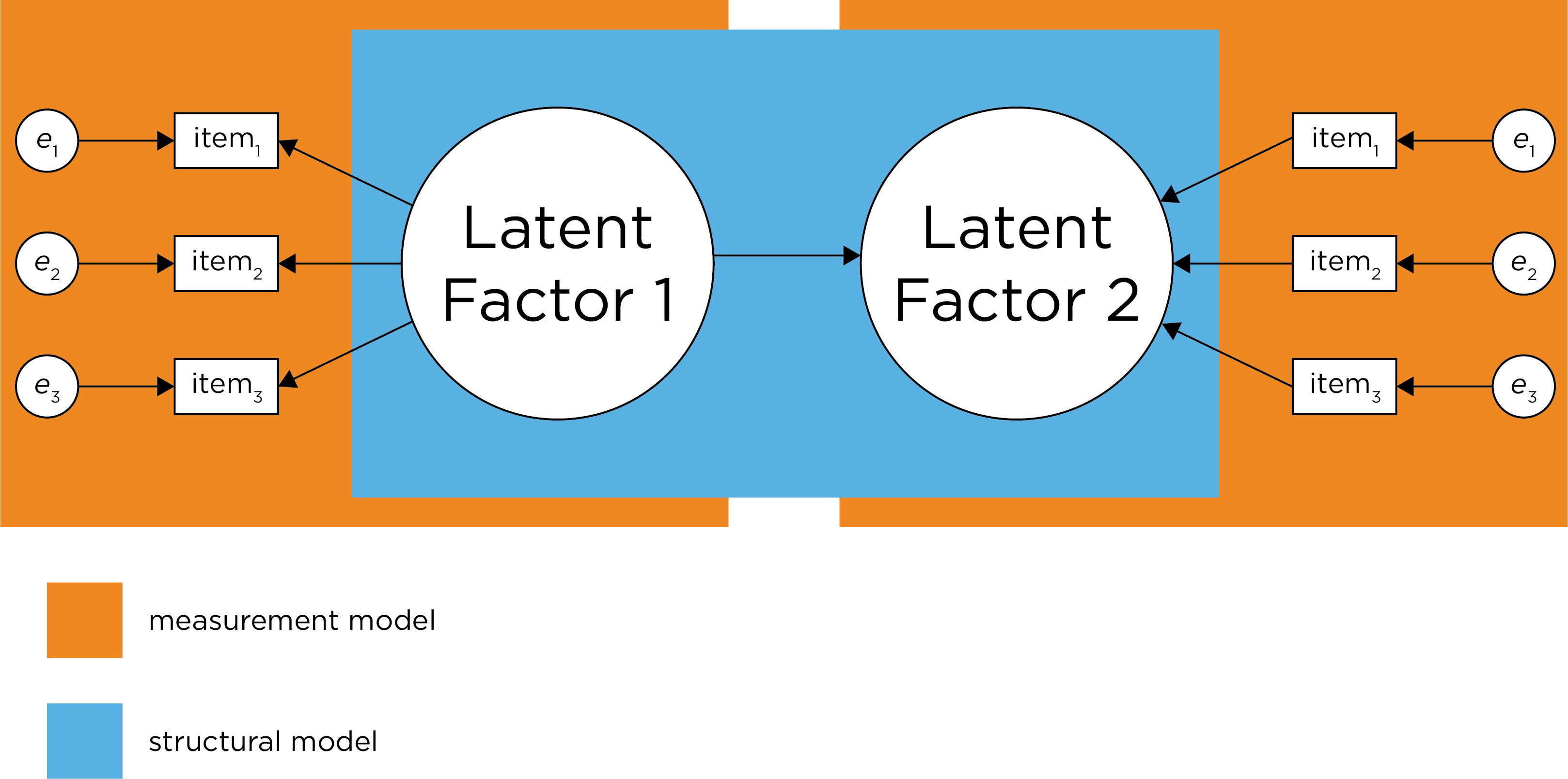
Figure 7.1: Demarcation Between Measurement Model and Structural Model. Disturbance term is zeta. (Figure adapted from Civelek (2018), Figure 1, p. 7. Civelek, M. E. (2018). Essentials of structural equation modeling. Zea E-Books. https://doi.org/10.13014/K2SJ1HR5)
SEM is flexible in allowing you to specify measurement error and correlated errors. Thus, you do not need the same assumptions as in classical test theory, which assumes that errors are random and uncorrelated. But the flexibility of SEM also poses challenges because you must explicitly decide what to include—and not include—in your model. This flexibility can be both a blessing and a curse. If the model fit is unacceptable, you can try fitting a different model to see which fits better. Nevertheless, it is important to use theory as a guide when specifying and comparing competing models, and not just rely solely on model fit comparison. For example, the model you fit should depend on how you conceptualize each construct: as reflective or formative.
7.4 Estimating Latent Factors
7.4.1 Model Identification
7.4.1.1 Types of Model Identification
There are important practical issues to consider with both reflective and formative models. An important practical issue is model identification—adding enough constraints so that there is only one, best answer. The model is identified when each of the estimated parameters has a unique solution. For ensuring the model is identifiable, see the criteria for identification of the measurement and structural model here (archived at https://perma.cc/5C9E-LBWM).
Degrees of freedom in a SEM model is the number of known values minus the number of estimated parameters. The number of known values in a SEM model is the number of variances and covariances in the variance-covariance matrix of the manifest (observed) variables in addition to the number of means (i.e., the number of manifest variables), which can be calculated as: \(\frac{m(m + 1)}{2} + m\), where \(m = \text{the number of manifest variables}\). You can never estimate more parameters than the number of known values. A model with zero degrees of freedom is considered “saturated”—it will have perfect fit because the model estimates as many parameters as there are known values. All things equal (i.e., in terms of model fit with the same number of manifest variables), a model with more degrees of freedom is preferred for its parsimony, because fewer parameters are estimated.
Based on the number of known values compared to the number of estimated parameters, a model can be considered either just identified, under-identified, or over-identified. A just identified model is a model in which the number of known values is equal to the number of parameters to be estimated (degrees of freedom = 0). An under-identified model is a model in which the number of known values is less than the number of parameters to be estimated (degrees of freedom < 0). An over-identified model is a model in which the number of known values is greater than the number of parameters to be estimated (degrees of freedom > 0).
As an example, there are 14 known values for a model with 4 manifest variables (\(\frac{4(4 + 1)}{2} + 4 = 14\)): 4 variances, 6 covariances, and 4 means.
Here is the variance-covariance matrix:
Code
         y1        y2        y3       y4
y1 6.387379        NA        NA       NA
y2 6.060140 16.424848        NA       NA
y3 5.613202  6.329419 11.066049       NA
y4 5.393572  9.910746  7.151898 11.22069
Here are the variances:
       y1        y2        y3        y4
 6.387379 16.424848 11.066049 11.220691
Here are the covariances:
Code
[1] 6.060140 5.613202 5.393572 6.329419 9.910746 7.151898Here are the means:
Code
      y1       y2       y3       y4
5.347059 4.284975 6.367156 4.356618
7.4.1.2 Approaches to Model Identification
The three most widely used approaches to identifying latent factors are:
7.4.1.2.1 Marker Variable Method
In the marker variable method, one of the indicators (i.e., manifest variables) is set to have a loading of 1. Here are examples of using the marker variable method for identification of a latent variable:
Code
markerVariable_syntax <- '
 #Factor loadings
 latentFactor =~ y1 + y2 + y3 + y4
'

markerVariable_fullSyntax <- '
 #Factor loadings
 latentFactor =~ 1*y1 + y2 + y3 + y4

 #Latent variance
 latentFactor ~~ latentFactor

 #Estimate residual variances of manifest variables
 y1 ~~ y1
 y2 ~~ y2
 y3 ~~ y3
 y4 ~~ y4

 #Estimate intercepts of manifest variables
 y1 ~ 1
 y2 ~ 1
 y3 ~ 1
 y4 ~ 1
'

markerVariableModelFit <- sem(
  markerVariable_syntax,
  data = PoliticalDemocracy,
  missing = "ML",
  estimator = "MLR")

markerVariableModelFit_full <- lavaan(
  markerVariable_fullSyntax,
  data = PoliticalDemocracy,
  missing = "ML",
  estimator = "MLR")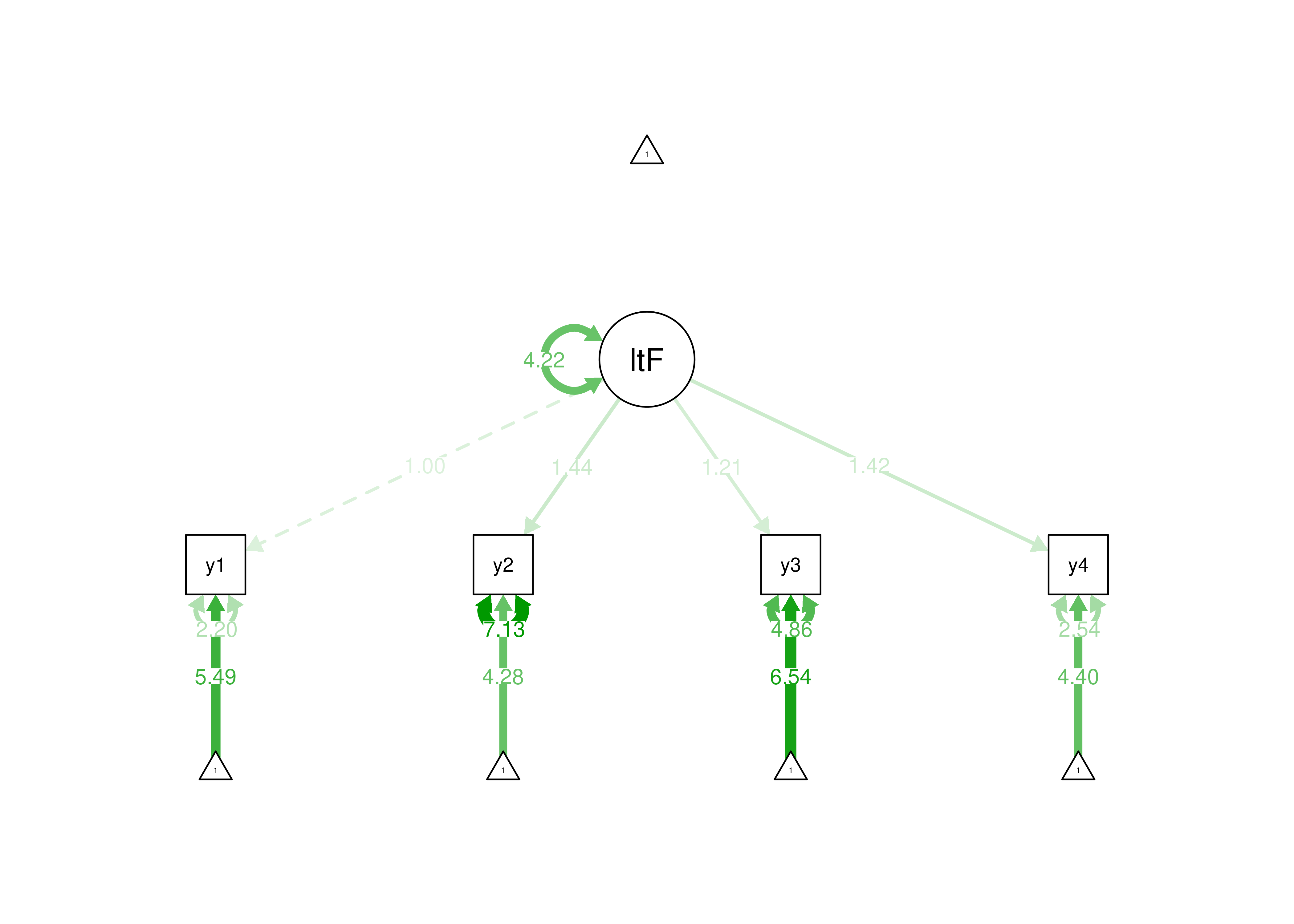
Figure 7.2: Identifying a Latent Variable Using the Marker Variable Approach.
7.4.1.2.2 Effects Coding Method
In the effects coding method, the average of the factor loadings is set to be 1. The effects coding method is useful if you are interested in the means or variances of the latent factor, because the metric of the latent factor is on the metric of the indicators. Here are examples of using the effects coding method for identification of a latent variable:
Code
effectsCoding_abbreviatedSyntax <- '
 #Factor loadings
 latentFactor =~ y1 + y2 + y3 + y4
'

effectsCoding_syntax <- '
 #Factor loadings
 latentFactor =~ NA*y1 + label1*y1 + label2*y2 + label3*y3 + label4*y4

 #Constrain factor loadings
 label1 == 4 - label2 - label3 - label4 # 4 = number of indicators
'

effectsCoding_fullSyntax <- '
 #Factor loadings
 latentFactor =~ label1*y1 + label2*y2 + label3*y3 + label4*y4

 #Constrain factor loadings
 label1 == 4 - label2 - label3 - label4 # 4 = number of indicators

 #Latent variance
 latentFactor ~~ latentFactor

 #Estimate residual variances of manifest variables
 y1 ~~ y1
 y2 ~~ y2
 y3 ~~ y3
 y4 ~~ y4

 #Estimate intercepts of manifest variables
 y1 ~ 1
 y2 ~ 1
 y3 ~ 1
 y4 ~ 1
'

effectsCodingModelFit_abbreviated <- sem(
  effectsCoding_abbreviatedSyntax,
  data = PoliticalDemocracy,
  effect.coding = "loadings",
  missing = "ML",
  estimator = "MLR")

effectsCodingModelFit <- sem(
  effectsCoding_syntax,
  data = PoliticalDemocracy,
  missing = "ML",
  estimator = "MLR")

effectsCodingModelFit_full <- lavaan(
  effectsCoding_fullSyntax,
  data = PoliticalDemocracy,
  missing = "ML",
  estimator = "MLR")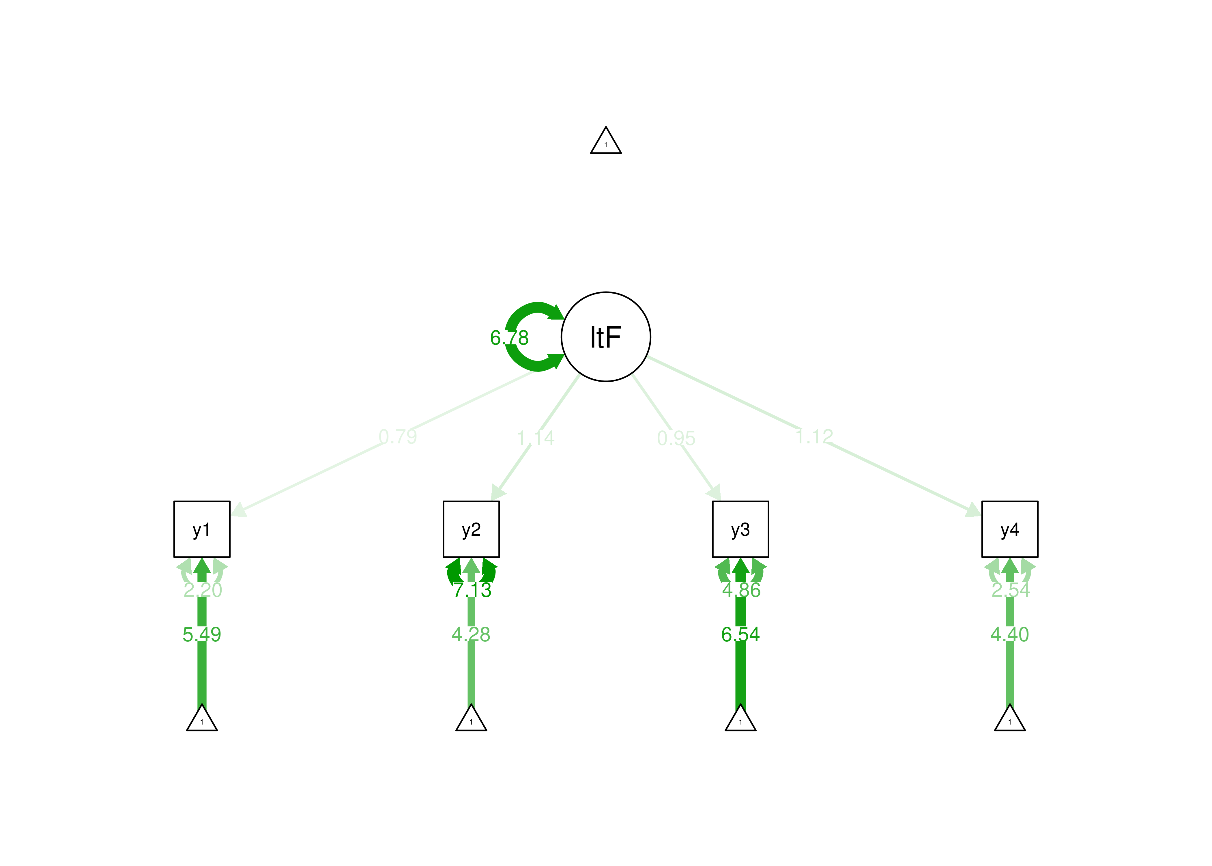
Figure 7.3: Identifying a Latent Variable Using the Effects Coding Approach.
7.4.1.2.3 Standardized Latent Factor Method
In the standardized latent factor method, the latent factor is set to have a mean of 0 and a standard deviation of 1. The standardized latent factor method is a useful approach if you are not interested in the means or variances of the latent factors and want to freely estimate the factor loadings. Here are examples of using the standardized latent factor method for identification of a latent variable:
Code
standardizedLatent_abbreviatedsyntax <- '
 #Factor loadings
 latentFactor =~ y1 + y2 + y3 + y4
'

standardizedLatent_syntax <- '
 #Factor loadings
 latentFactor =~ NA*y1 + y2 + y3 + y4

 #Latent mean
 latentFactor ~ 0

 #Latent variance
 latentFactor ~~ 1*latentFactor
'

standardizedLatent_fullSyntax <- '
 #Factor loadings
 latentFactor =~ NA*y1 + y2 + y3 + y4

 #Latent mean
 latentFactor ~ 0

 #Latent variance
 latentFactor ~~ 1*latentFactor

 #Estimate residual variances of manifest variables
 y1 ~~ y1
 y2 ~~ y2
 y3 ~~ y3
 y4 ~~ y4

 #Estimate intercepts of manifest variables
 y1 ~ 1
 y2 ~ 1
 y3 ~ 1
 y4 ~ 1
'

standardizedLatentFit_abbreviated <- sem(
  standardizedLatent_abbreviatedsyntax,
  data = PoliticalDemocracy,
  std.lv = TRUE,
  missing = "ML",
  estimator = "MLR")

standardizedLatentFit <- sem(
  standardizedLatent_syntax,
  data = PoliticalDemocracy,
  missing = "ML",
  estimator = "MLR")

standardizedLatentFit_full <- lavaan(
  standardizedLatent_fullSyntax,
  data = PoliticalDemocracy,
  missing = "ML",
  estimator = "MLR")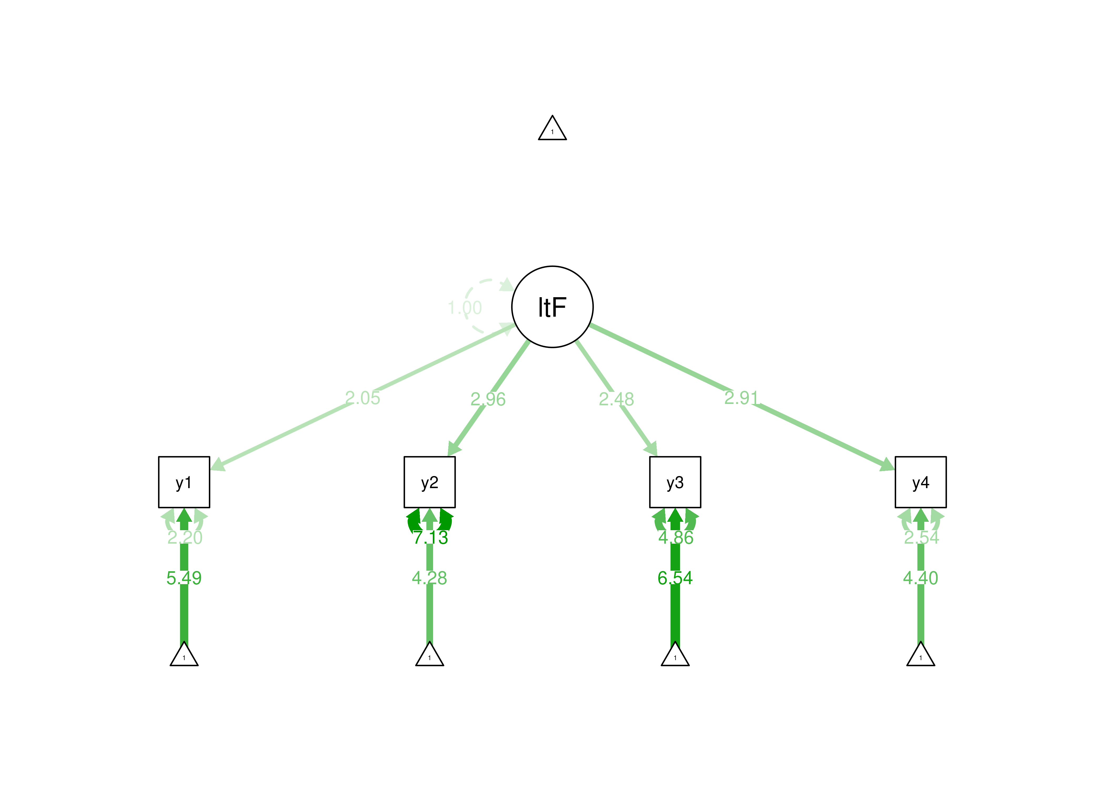
Figure 7.4: Identifying a Latent Variable Using the Standardized Latent Factor Approach.
7.4.2 Types of Latent Factors
7.4.2.1 Reflective Latent Factors
For a reflective model with 4 indicators, we would need to estimate 12 parameters: a factor loading, error term, and intercept for each of the 4 indicators. Here are the parameters estimated:
Code
reflectiveModel_syntax <- '
 #Reflective model factor loadings
 reflective =~ y1 + y2 + y3 + y4
'

reflectiveModelFit <- sem(
  reflectiveModel_syntax,
  data = PoliticalDemocracy,
  missing = "ML",
  estimator = "MLR",
  std.lv = TRUE)

reflectiveModelParameters <- parameterEstimates(
  reflectiveModelFit)[!is.na(parameterEstimates(reflectiveModelFit)$z),]

row.names(reflectiveModelParameters) <- NULL

reflectiveModelParameters
Here are the degrees of freedom:
df
 2
Here is a model diagram:
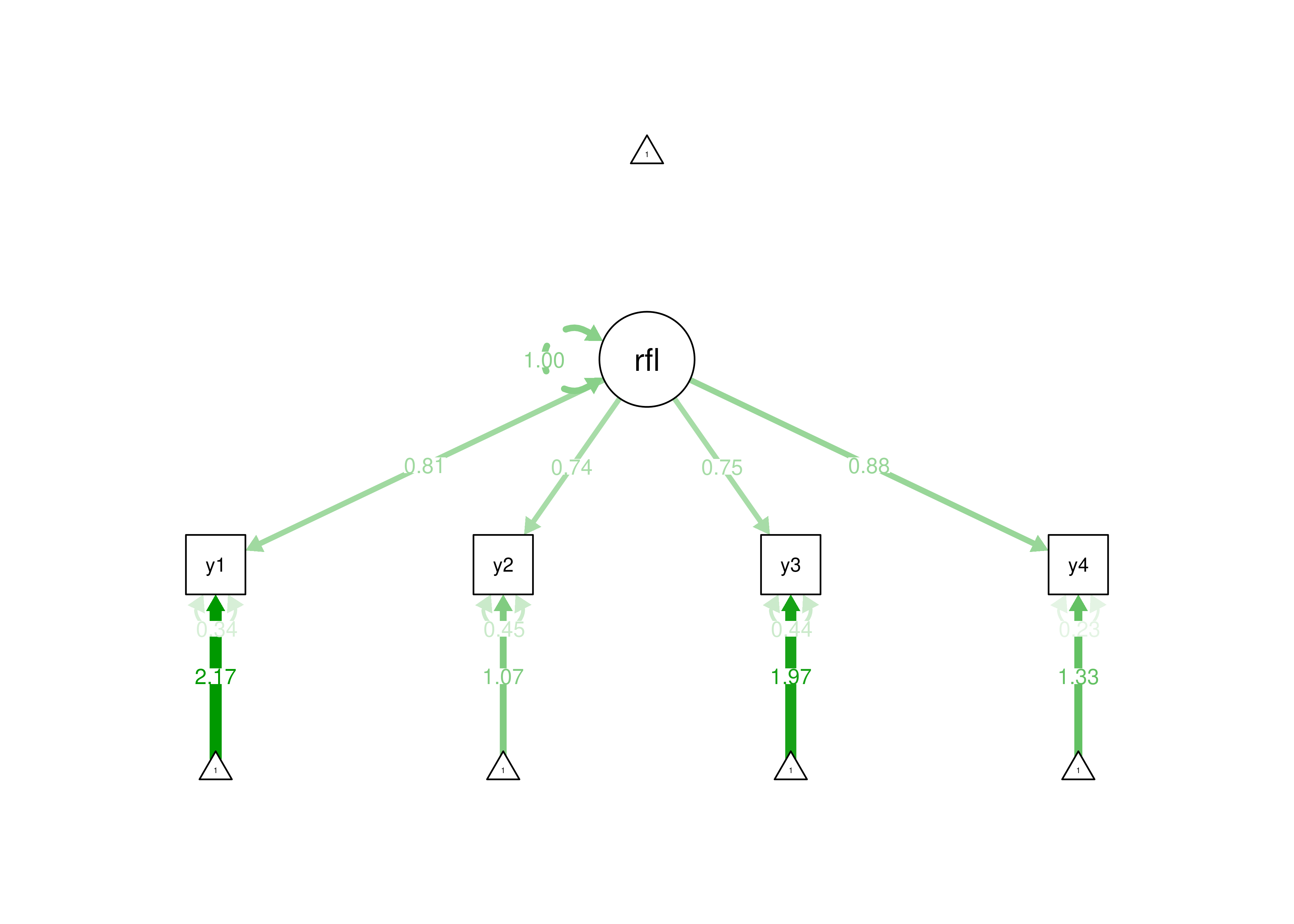
Figure 7.5: Example of a Reflective Model.
Thus, for a reflective model, we only have to estimate a small number of parameters to specify what is happening in our model, so the model is parsimonious. With 4 indicators, the number of known values (14) is greater than the number of parameters (12). We have 2 degrees of freedom (\(14 - 12 = 2\)). Because the degrees of freedom is greater than 0, it is easy to identify the model—the model is over-identified. A reflective model with 3 indicators would have 9 known values (\(\frac{3(3 + 1)}{2} + 3 = 9\)), 9 parameters (3 factor loadings, 3 error terms, 3 intercepts), and 0 degrees of freedom, and it would be identifiable because it would be just-identified.
7.4.2.2 Formative Latent Factors
However, for a formative model, we must specify more parameters: a factor loading, intercept, and variance for each of the 4 indicators, all 6 permissive correlations, and 1 error term for the latent variable, for a total of 19 parameters. Here are the parameters estimated:
Code
formativeModel_syntax <- '
 #Formative model factor loadings
 formative <~ v1 + v2 + v3 + v4

 formative ~~ formative
'

formativeModelFit <- sem(
  formativeModel_syntax,
  data = PoliticalDemocracy,
  missing = "ML",
  estimator = "MLR",
  optim.gradient = "numerical")

formativeModelParameters <- parameterEstimates(formativeModelFit)

formativeModelParameters
Here are the degrees of freedom:
Code
[1] 0lavaan 0.6-20 ended normally after 7 iterations
Estimator ML
Optimization method NLMINB
Number of model parameters 7
Number of observations 75
Number of missing patterns 10
Model Test User Model:
Test statistic NA
Degrees of freedom -3
P-value (Unknown) NAHere is a model diagram:
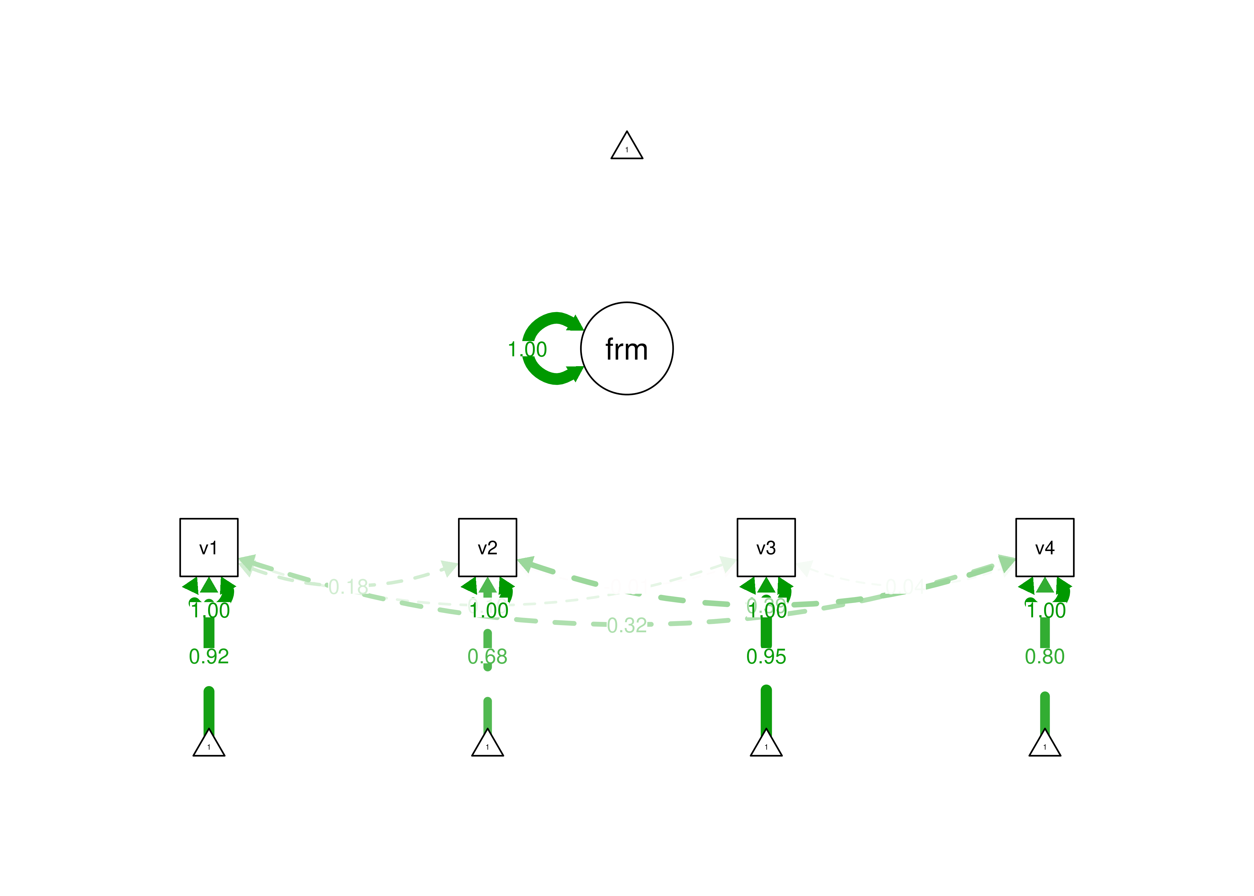
Figure 7.6: Example of an Under-Identified Formative Model.
For a formative model with 4 measures, the number of known values (14) is less than the number of parameters (19). The number of degrees of freedom is negative (\(14 - 19 = -5\)), thus the model is not able to be identified—the model is under-identified.
Thus, for a formative model, we need more parameters than we have data—the model is under-identified. Therefore, to estimate a formative model with 4 indicators, we must add assumptions and other variables that are consequences of the formative construct. Options for identifying a formative construct are described by Treiblmaier et al. (2011). See below for an example formative model that is identified because of additional assumptions.
Code
formativeModel2_syntax <- '
 #Formative model factor loadings
 formative <~ 1*v1 + v2 + v3 + v4
 reflective =~ y1 + y2 + y3 + y4

 formative ~~ 1*formative
 reflective ~ formative
'

formativeModel2Fit <- sem(
  formativeModel2_syntax,
  data = PoliticalDemocracy,
  missing = "ML",
  estimator = "MLR",
  optim.gradient = "numerical")

formativeModel2Parameters <- parameterEstimates(formativeModel2Fit)
formativeModel2Parametersdf
14 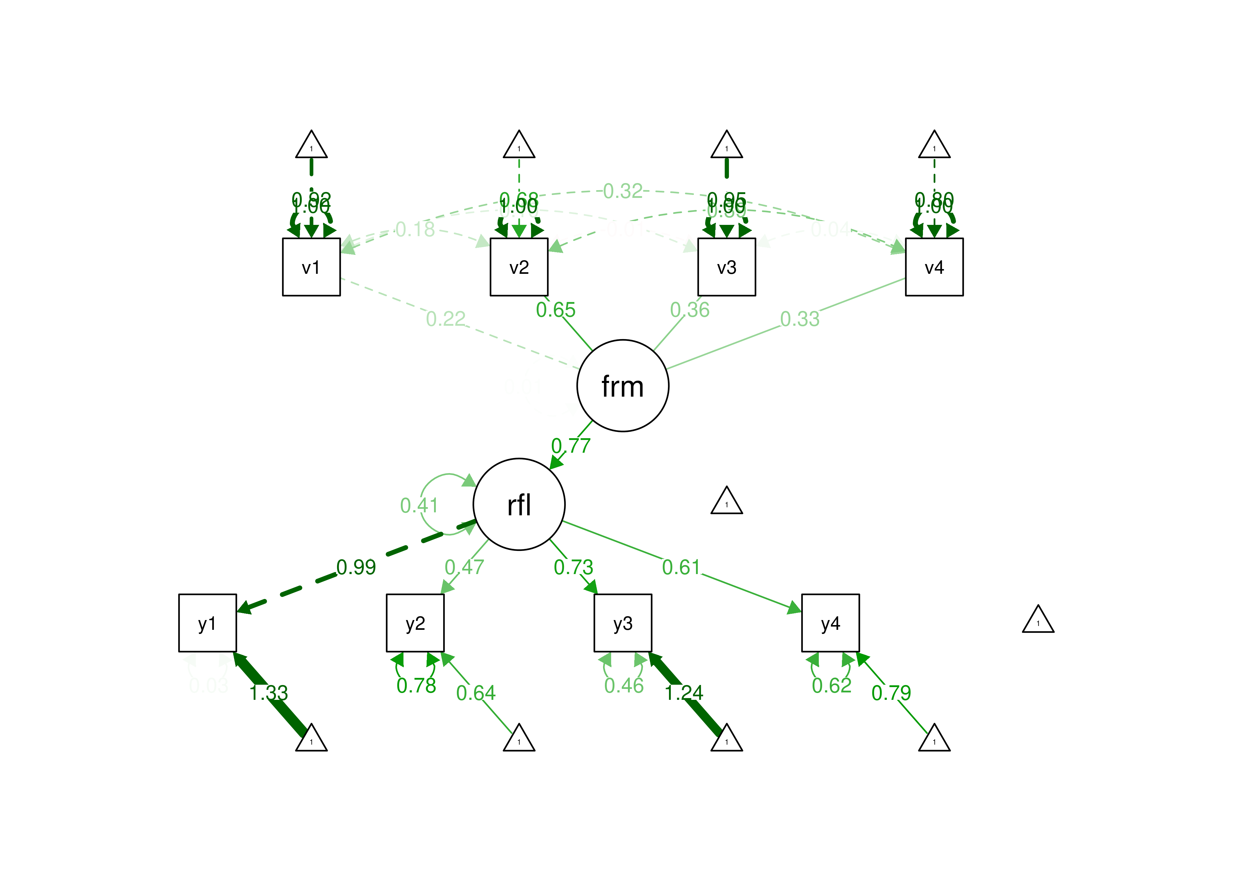
Figure 7.7: Example of an Identified Formative Model.
Thus, formative constructs are challenging to use in a SEM framework. To estimate a formative construct in a SEM framework, the formative construct must be used in the context of a model that allows some constraints. A formative latent factor includes a disturbance term, and is thus not entirely determined by the causal indicators (Bollen & Bauldry, 2011). A composite (such as in principal component analysis), by contrast, has no disturbance term and is therefore completely determined by the composite indicators (Bollen & Bauldry, 2011). Emerging techniques such as confirmatory composite analysis allow estimation of formative composites (Schuberth, 2023; Yu et al., 2023).
Below is an example of confirmatory composite analysis using the Henseler-Ogasawara specification (adapted from: https://confirmatorycompositeanalysis.com/tutorials-lavaan; archived at: https://perma.cc/7LSU-PTZR) (Schuberth, 2023):
Code
formativeModel3_syntax <- '
  # Specification of the reflective latent factor

  reflective =~ y1 + y2 + y3 + y4

  # Specification of the associations between the observed variables v1 - v4
  # and the emergent variable "formative" in terms of composite loadings.

  formative =~ NA*v1 + l11*v1+ l21*v2 + 1*v3 + l41*v4

  # Label the variance of the formative composite

  formative ~~ varformative*formative

  # Specification of the associations between the observed variables v1 - v4
  # and their excrescent variables in terms of composite loadings.

  nu11 =~ 1*v1 + l22*v2 + l32*v3 + l42*v4
  nu12 =~ 0*v1 + 1*v2 + l33*v3 + l43*v4
  nu13 =~ 0*v1 + 0*v2 + l34*v3 + 1*v4

  # Label the variances of the excrescent variables

  nu11 ~~ varnu11*nu11
  nu12 ~~ varnu12*nu12
  nu13 ~~ varnu13*nu13

  # Specify the effect of formative on reflective

  reflective ~ formative

  # The H-O specification assumes that the excrescent variables are uncorrelated.
  # Therefore, the covariance between the excrescent variables is fixed to 0:

  nu11 ~~ 0*nu12 + 0*nu13
  nu12 ~~ 0*nu13

  # Moreover, the H-O specification assumes that the excrescent variables are uncorrelated
  # with the emergent and latent variables. Therefore, the covariances between
  # the emergent and the excrescent varibales are fixed to 0:

  formative ~~ 0*nu11 + 0*nu12 + 0*nu13

  reflective =~ 0*nu11 + 0*nu12 + 0*nu13

  # In lavaan, the =~ command is originally used to specify a common factor model,
  # which assumes that each observed variable is affected by a random measurement error.
  # It is assumed that the observed variables forming composites are free from
  # random measurement error. Therefore, the variances of the random measurement errors
  # originally attached to the observed variables by the common factor model are fixed to 0:

  v1 ~~ 0*v1
  v2 ~~ 0*v2
  v3 ~~ 0*v3
  v4 ~~ 0*v4

  # Calculate the unstandardized weights to form the formative latent variable

  w1 := (-l32 + l22*l33 + l34*l42 - l22*l34*l43)/(1 -
      l11*l32 - l21*l33 + l11*l22*l33 - l34*l41 + l11*l34*l42 +
     l21* l34* l43 - l11* l22* l34* l43)
  w2 := (-l33 + l34*l43)/(1 - l11*l32 - l21*l33 +
      l11*l22*l33 - l34*l41 + l11*l34*l42 + l21*l34*l43 - l11*l22*l34*l43)
  w3 := 1/(1 - l11*l32 - l21*l33 + l11*l22*l33 -
      l34*l41 + l11*l34*l42 + l21*l34*l43 - l11*l22*l34*l43)
  w4 := -l34/(1 - l11*l32 - l21*l33 + l11*l22*l33 -
      l34*l41 + l11*l34*l42 + l21*l34*l43 - l11*l22*l34*l43)

  # Calculate the variances

  varv1 := l11^2*varformative + varnu11
  varv2 := l21^2*varformative + l22^2*varnu11 + varnu12
  varv3 := varformative + l32^2*varnu11 + l33^2*varnu12 + l34^2*varnu13
  varv4 := l41^2*varformative + l42^2*varnu11 + l43^2*varnu12 + varnu13

  # Calculate the standardized weights to form the formative latent variable

  w1std := w1*(varv1/varformative)^(1/2)
  w2std := w2*(varv2/varformative)^(1/2)
  w3std := w3*(varv3/varformative)^(1/2)
  w4std := w4*(varv4/varformative)^(1/2)
'

formativeModel3Fit <- sem(
  formativeModel3_syntax,
  data = PoliticalDemocracy,
  missing = "ML",
  estimator = "MLR")

formativeModel3Parameters <- parameterEstimates(formativeModel3Fit)
formativeModel3Parametersdf
14 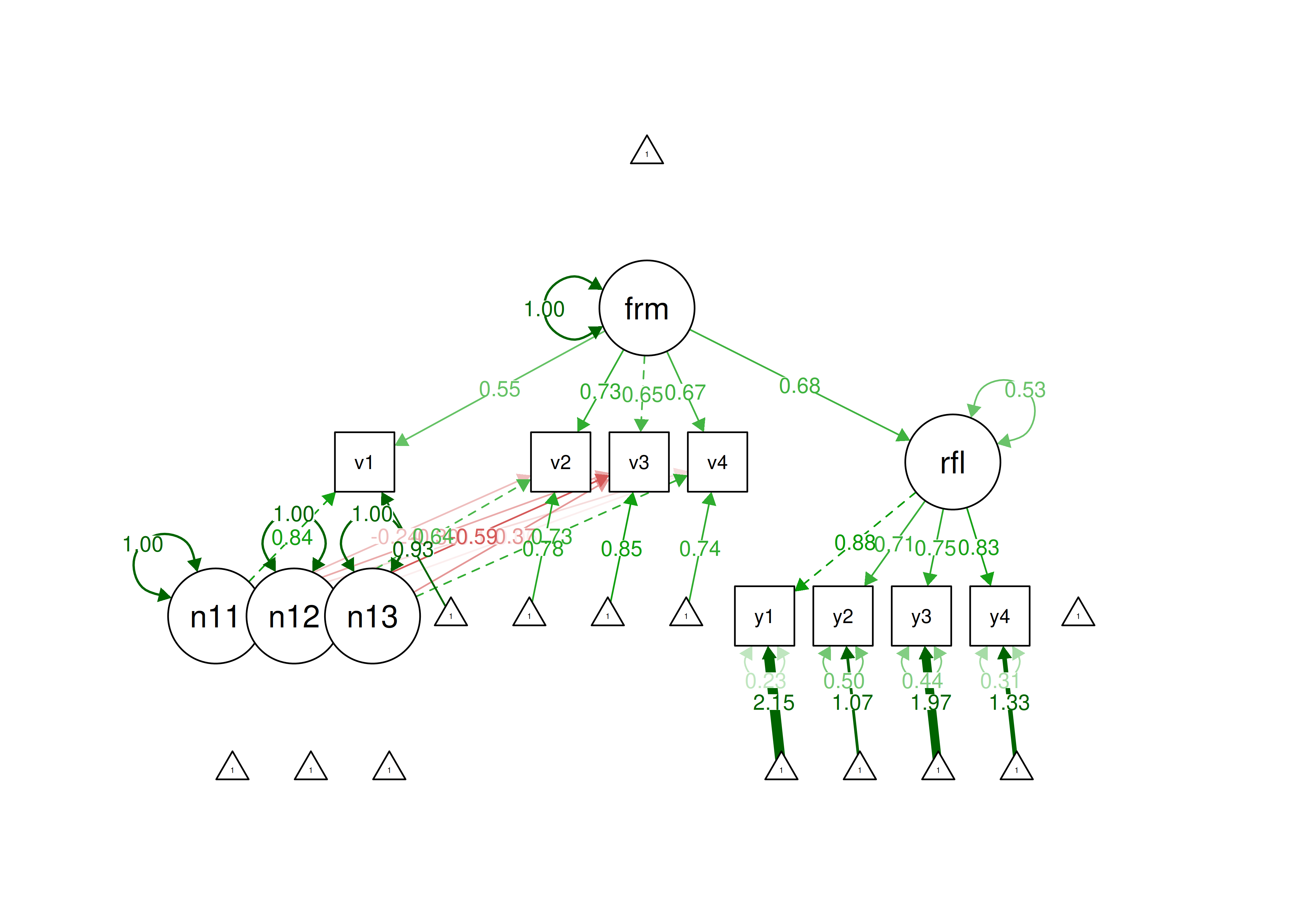
Below is an example of confirmatory composite analysis using the refined Henseler-Ogasawara specification (Yu et al., 2023):
Code
formativeModel4_syntax <- '
  # Specification of the reflective latent factor

  reflective =~ y1 + y2 + y3 + y4

  # Specification of the associations between the observed variables v1 - v4
  # and the emergent variable "formative" in terms of composite loadings.

  formative =~ NA*v1 + l11*v1 + l21*v2 + 1*v3 + l41*v4

  # Label the variance of the formative composite

  formative ~~ varformative*formative

  # Specification of the associations between the observed variables v1 - v4
  # and their excrescent variables in terms of composite loadings.

  nu1 =~ 1*v2 + l12*v1
  nu2 =~ 1*v3 + l23*v2
  nu3 =~ 1*v4 + l34*v3

  # Label the variances of the excrescent variables

  nu1 ~~ varnu1*nu1
  nu2 ~~ varnu2*nu2
  nu3 ~~ varnu3*nu3

  # Specify the effect of formative on reflective

  reflective ~ formative

  # Constrain the covariances between excrescent variables and
  # other variables in the structural model to zero. Moreover,
  # label the covariances among excrescent variables.

  nu1 ~~ 0*formative + 0*reflective + cov12*nu2 + cov13*nu3
  nu2 ~~ 0*formative + 0*reflective + cov23*nu3
  nu3 ~~ 0*formative + 0*reflective

  # Fix the variances of the disturbance terms to zero.

  v1 ~~ 0*v1
  v2 ~~ 0*v2
  v3 ~~ 0*v3
  v4 ~~ 0*v4

  # Calculate the unstandardized weights to form the formative latent variable

  w1 := ((1)*((1)*((1)))) / ((l11)*((1)*((1)*((1)))) + -(l21)*((l12)*((1)*((1)))) + (1)*((l12)*((l23)*((1)))) + -(l41)*((l12)*((l23)*((l34)))))
  w2 := -((l12)*((1)*((1)))) / ((l11)*((1)*((1)*((1)))) + -(l21)*((l12)*((1)*((1)))) + (1)*((l12)*((l23)*((1)))) + -(l41)*((l12)*((l23)*((l34)))))
  w3 := ((l12)*((l23)*((1)))) / ((l11)*((1)*((1)*((1)))) + -(l21)*((l12)*((1)*((1)))) + (1)*((l12)*((l23)*((1)))) + -(l41)*((l12)*((l23)*((l34)))))
  w4 := -((l12)*((l23)*((l34)))) / ((l11)*((1)*((1)*((1)))) + -(l21)*((l12)*((1)*((1)))) + (1)*((l12)*((l23)*((1)))) + -(l41)*((l12)*((l23)*((l34)))))

  # Calculate the variances

  varv1 := ((l11) * (varformative)) * (l11) + ((l12) * (varnu1)) * (l12)
  varv2 := ((l21) * (varformative)) * (l21) + ((1) * (varnu1) + (l23) * (cov12)) * (1) + ((1) * (cov12) + (l23) * (varnu2)) * (l23)
  varv3 := ((1) * (varformative)) * (1) + ((1) * (varnu2) + (l34) * (cov23)) * (1) + ((1) * (cov23) + (l34) * (varnu3)) * (l34)
  varv4 := ((l41) * (varformative)) * (l41) + ((1) * (varnu3)) * (1)

  # Calculate the standardized weights to form the formative latent variable

  wstdv1 := ((w1) * (sqrt(varv1))) * (1/sqrt(varformative))
  wstdv2 := ((w2) * (sqrt(varv2))) * (1/sqrt(varformative))
  wstdv3 := ((w3) * (sqrt(varv3))) * (1/sqrt(varformative))
  wstdv4 := ((w4) * (sqrt(varv4))) * (1/sqrt(varformative))
'

formativeModel4Fit <- sem(
  formativeModel4_syntax,
  data = PoliticalDemocracy,
  missing = "ML",
  estimator = "MLR")

formativeModel4Parameters <- parameterEstimates(formativeModel4Fit)
formativeModel4Parametersdf
14 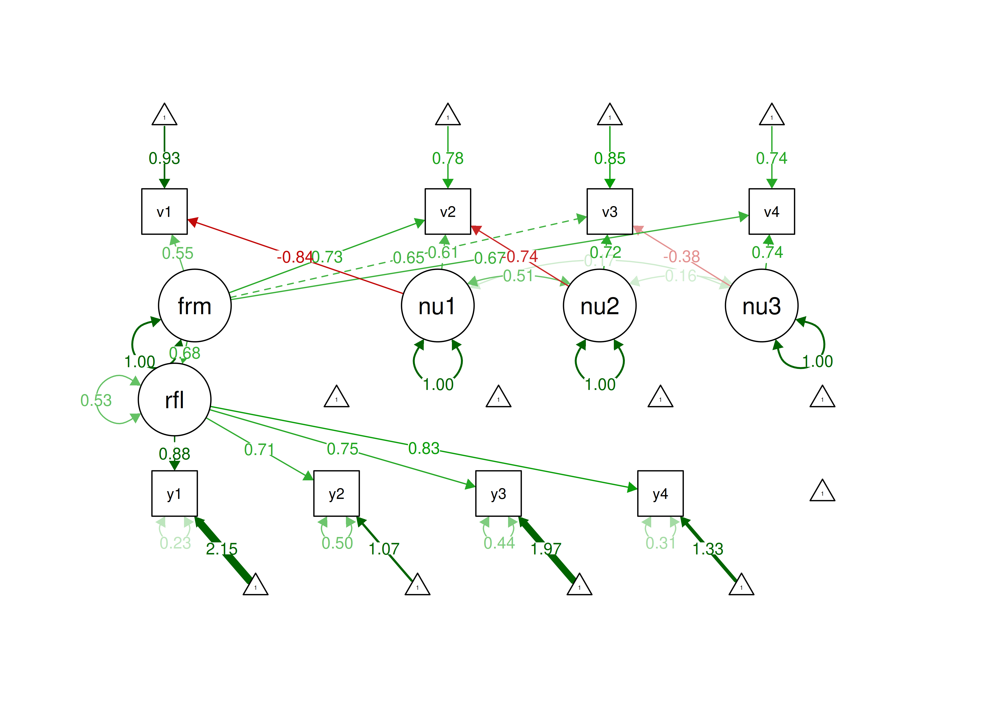
You can generate the weights for the indicators (to be used in the model syntax) for the refined Henseler-Ogasawara specification using the following code:
Code
library("calculus")

# First, construct the loading matrix
loadingMatrix <- matrix(c('l11','l21',1,'l41','l12',1,0,0,0,'l23',1,0,0,0,'l34',1),4,4)

# Check the structure
loadingMatrix

# Invert matrix, the first row contains the (unstandardized) weights
# these can be copy and pasted to the lavaan model to specify the weights as new parameters
mxinv(loadingMatrix)
Florian Schubert provides an R function to create the full lavaan syntax for confirmatory composite analysis at the following link: https://github.com/FloSchuberth/HOspecification
7.5 Additional Types of SEM
Up to this point, we have discussed SEM with dimensional constructs. It also worth knowing about additional types of SEM models, including latent class models and mixture models, that handle categorical constructs. However, most disorders are more accurately conceptualized as dimensional than as categorical (Markon et al., 2011), so just because you can estimate categorical latent factors does not necessarily mean that one should.
7.5.1 Latent Class Models
In latent class models, the construct is not dimensional, but rather categorical. The categorical constructs are latent classifications and are called latent classes. For instance, the construct could be a diagnosis that influences scores on the measures. Latent class models examine qualitative differences in kind, rather than quantitative differences in degree.
7.5.2 Mixture Models
Mixture models allow for a combination of latent categorical constructs (classes) and latent dimensional constructs. That is, it allows for both qualitative and quantitative differences. However, this additional model complexity also necessitates a larger sample size for estimation. SEM generally requires a 3-digit sample size (\(N = 100+\)), whereas mixture models typically require a 4- or 5-digit sample size (\(N = 1,000+\)).
7.5.3 Exploratory Structural Equation Models
We describe exploratory structural equation models in Section 14.1.4.3.3.
7.6 Causal Diagrams: Directed Acyclic Graphs
A key tool when designing a structural equation model is a conceptual depiction of the hypothesized causal processes.
A causal diagram depicts the hypothesized causal processes that link two or more variables.
A common form of causal diagrams is the directed acyclic graph (DAG).
DAGs provide a helpful tool to communicate about causal questions and help identify how to avoid bias (i.e., over-estimation) in associations between variables due to confounding (i.e., common causes) (Digitale et al., 2022).
Free tools to create DAGs include the R package dagitty (Textor et al., 2017) and the associated browser-based extension, DAGitty: https://dagitty.net (archived at https://perma.cc/U9BY-VZE2).
Path analytic diagrams (i.e., causal diagrams with boxes, circles, and lines) are described in Section 4.1.1 of Chapter 4.
Karch (in press) provides a tool to create lavaan R syntax from a path analytic diagram: https://lavaangui.org.
7.7 Model Fit Indices
Various model fit indices can be used for evaluating how well a model fits the data and for comparing the fit of two competing models. Fit indices known as absolute fit indices compare whether the model fits better than the best-possible fitting model (i.e., a saturated model). Examples of absolute fit indices include the chi-square test, root mean square error of approximation (RMSEA), and the standardized root mean square residual (SRMR).
The chi-square test evaluates whether the model has a significant degree of misfit relative to the best-possible fitting model (a saturated model that fits as many parameters as possible; i.e., as many parameters as there are degrees of freedom); the null hypothesis of a chi-square test is that there is no difference between the predicted data (i.e., the data that would be observed if the model were true) and the observed data. Thus, a non-significant chi-square test indicates good model fit. However, because the null hypothesis of the chi-square test is that the model-implied covariance matrix is exactly equal to the observed covariance matrix (i.e., a model of perfect fit), this may be an unrealistic comparison. Models are simplifications of reality, and our models are virtually never expected to be a perfect description of reality. Thus, we would say a model is “useful” and partially validated if “it helps us to understand the relation between variables and does a ‘reasonable’ job of matching the data…A perfect fit may be an inappropriate standard, and a high chi-square estimate may indicate what we already know—that the hypothesized model holds approximately, not perfectly.” (Bollen, 1989, p. 268). The power of the chi-square test depends on sample size, and a large sample will likely detect small differences as significantly worse than the best-possible fitting model (Bollen, 1989).
RMSEA is an index of absolute fit. Lower values indicate better fit.
SRMR is an index of absolute fit with no penalty for model complexity. Lower values indicate better fit.
There are also various fit indices known as incremental, comparative, or relative fit indices that compare whether the model fits better than the worst-possible fitting model (i.e., a “baseline” or “null” model). Incremental fit indices include a chi-square difference test, the comparative fit index (CFI), and the Tucker-Lewis index (TLI). Unlike the chi-square test comparing the model to the best-possible fitting model, a significant chi-square test of the relative fit index indicates better fit—i.e., that the model fits better than the worst-possible fitting model.
CFI is another relative fit index that compares the model to the worst-possible fitting model. Higher values indicate better fit.
TLI is another relative fit index. Higher values indicate better fit.
Parsimony fit include fit indices that use information criteria fit indices, including the Akaike Information Criterion (AIC) and the Bayesian Information Criterion (BIC). BIC penalizes model complexity more so than AIC. Lower AIC and BIC values indicate better fit.
Chi-square difference tests and CFI can be used to compare two nested models. AIC and BIC can be used to compare two non-nested models.
Criteria for acceptable fit and good fit of SEM models are in Table 7.1.
In addition, dynamic fit indexes have been proposed based on simulation to identify fit index cutoffs that are tailored to the characteristics of the specific model and data (McNeish, 2026; McNeish & Wolf, 2023); dyanmic fit indexes are available via the dynamic package in R or with a webapp.
| SEM Fit Index | Acceptable Fit | Good Fit |
|---|---|---|
| RMSEA | \(\leq\) .08 | \(\leq\) .05 |
| CFI | \(\geq\) .90 | \(\geq\) .95 |
| TLI | \(\geq\) .90 | \(\geq\) .95 |
| SRMR | \(\leq\) .10 | \(\leq\) .08 |
However, good model fit does not necessarily indicate a true model.
In addition to global fit indices, it can also be helpful to examine evidence of local fit (Kline, 2023; McNeish, 2026), such as the residual covariance matrix. The residual covariance matrix represents the difference between the observed covariance matrix and the model-implied covariance matrix (the observed covariance matrix minus the model-implied covariance matrix). These difference values are called covariance residuals. Standardizing the covariance matrix by converting each to a correlation matrix can be helpful for interpreting the magnitude of any local misfit. This is known as a residual correlation matrix, which is composed of correlation residuals. Correlation residuals greater than |.10| are possible evidence for poor local fit (Kline, 2023). If a correlation residual is positive, it suggests that the model underpredicts the observed association between the two variables (i.e., the observed covariance is greater than the model-implied covariance). If a correlation residual is negative, it suggests that the model overpredicts their observed association between the two variables (i.e., the observed covariance is smaller than the model-implied covariance). If the two variables are connected by only indirect pathways, it may be helpful to respecify the model with direct pathways between the two variables, such as a direct effect (i.e., regression path) or a covariance path. For guidance on evaluating local fit, see Kline (2024).
7.8 Correlation Matrix
          measure1  measure2  measure3
measure1 1.0000000 0.5444728 0.6782616
measure2 0.5444728 1.0000000 0.7766733
measure3 0.6782616 0.7766733 1.0000000
Correlation matrices of various types using the cor.table() function from the petersenlab package (Petersen, 2025) are in Tables 7.2, 7.3, and 7.4.
Code
| measure1 | measure2 | measure3 | |
|---|---|---|---|
| 1. measure1.r | 1.00 | .54*** | .68*** |
| 2. sig | NA | .00 | .00 |
| 3. n | 298 | 297 | 298 |
| 4. measure2.r | .54*** | 1.00 | .78*** |
| 5. sig | .00 | NA | .00 |
| 6. n | 297 | 298 | 298 |
| 7. measure3.r | .68*** | .78*** | 1.00 |
| 8. sig | .00 | .00 | NA |
| 9. n | 298 | 298 | 299 |
| measure1 | measure2 | measure3 | |
|---|---|---|---|
| 1. measure1 | 1.00 | ||
| 2. measure2 | .54*** | 1.00 | |
| 3. measure3 | .68*** | .78*** | 1.00 |
| measure1 | measure2 | measure3 | |
|---|---|---|---|
| 1. measure1 | 1.00 | ||
| 2. measure2 | .54 | 1.00 | |
| 3. measure3 | .68 | .78 | 1.00 |
7.9 Measurement Model (of a Given Construct)
Even though CFA models are measurement models, I provide separate examples of a measurement model and CFA models in my examples because CFA is often used to test competing factor structures. For instance, you could use CFA to test whether the variance in several measures’ scores is best explained with one factor or two factors. In the measurement model below, I present a simple one-factor model with three measures. The measurement model is what we settle on as the estimation of each construct before we add the structural component to estimate the relations among latent variables. Basically, we add the structural component onto the measurement model. In Section 7.10, I present a CFA model with multiple latent factors.
The measurement models were fit in the lavaan package (Rosseel et al., 2022).
7.9.1 Specify the Model
Code
measurementModel_syntax <- '
 #Factor loadings
 latentFactor =~ measure1 + measure2 + measure3
'

measurementModel_fullSyntax <- '
 #Factor loadings (free the factor loading of the first indicator)
 latentFactor =~ NA*measure1 + measure2 + measure3

 #Fix latent mean to zero
 latentFactor ~ 0

 #Fix latent variance to one
 latentFactor ~~ 1*latentFactor

 #Estimate covariances among latent variables (not applicable because there is only one latent variable)

 #Estimate residual variances of manifest variables
 measure1 ~~ measure1
 measure2 ~~ measure2
 measure3 ~~ measure3

 #Free intercepts of manifest variables
 measure1 ~ int1*1
 measure2 ~ int2*1
 measure3 ~ int3*1
'7.9.3 Display Summary Output
This measurement model with three indicators is just-identified—the number of parameters estimated is equal to the number of known values, thus leaving 0 degrees of freedom. In the model, all three indicators load strongly on the latent factor (measure 1: \(\beta = 0.69\); measure 2: \(\beta = 0.79\); measure 3: \(\beta = 0.98\)). Thus, the loadings of this measurement model would be consistent with a reflective latent construct. In terms of interpretation, all three indicators loaded positively on the latent factor, so higher levels of the latent factor are indicated by higher levels on the indicators. However, one of the estimated observed variances is negative, so the model is not able to be estimated accurately. Thus, we would need to make additional adjustments in order to estimate the model.
lavaan 0.6-20 ended normally after 23 iterations

  Estimator                                         ML
  Optimization method                           NLMINB
  Number of model parameters                         9

                                                  Used       Total
  Number of observations                           299         300
  Number of missing patterns                         3

Model Test User Model:
                                              Standard      Scaled
  Test Statistic                                 0.000       0.000
  Degrees of freedom                                 0           0

Model Test Baseline Model:

  Test statistic                               459.500     389.896
  Degrees of freedom                                 3           3
  P-value                                        0.000       0.000
  Scaling correction factor                                  1.179

User Model versus Baseline Model:

  Comparative Fit Index (CFI)                    1.000       1.000
  Tucker-Lewis Index (TLI)                       1.000       1.000

  Robust Comparative Fit Index (CFI)                         1.000
  Robust Tucker-Lewis Index (TLI)                            1.000

Loglikelihood and Information Criteria:

  Loglikelihood user model (H0)              -3588.224   -3588.224
  Loglikelihood unrestricted model (H1)      -3588.224   -3588.224

  Akaike (AIC)                                7194.449    7194.449
  Bayesian (BIC)                              7227.753    7227.753
  Sample-size adjusted Bayesian (SABIC)       7199.210    7199.210

Root Mean Square Error of Approximation:

  RMSEA                                          0.000          NA
  90 Percent confidence interval - lower         0.000          NA
  90 Percent confidence interval - upper         0.000          NA
  P-value H_0: RMSEA <= 0.050                       NA          NA
  P-value H_0: RMSEA >= 0.080                       NA          NA

  Robust RMSEA                                               0.000
  90 Percent confidence interval - lower                     0.000
  90 Percent confidence interval - upper                     0.000
  P-value H_0: Robust RMSEA <= 0.050                            NA
  P-value H_0: Robust RMSEA >= 0.080                            NA

Standardized Root Mean Square Residual:

  SRMR                                           0.000       0.000

Parameter Estimates:

  Standard errors                             Sandwich
  Information bread                           Observed
  Observed information based on                Hessian

Latent Variables:
                   Estimate  Std.Err  z-value  P(>|z|)   Std.lv  Std.all
  latentFactor =~
    measure1          7.198    0.575   12.525    0.000    7.198    0.689
    measure2         13.487    0.855   15.780    0.000   13.487    0.789
    measure3         28.122    1.343   20.943    0.000   28.122    0.984

Intercepts:
                   Estimate  Std.Err  z-value  P(>|z|)   Std.lv  Std.all
   .measure1         50.136    0.605   82.859    0.000   50.136    4.797
   .measure2         50.489    0.990   51.024    0.000   50.489    2.952
   .measure3         99.720    1.652   60.361    0.000   99.720    3.491

Variances:
                   Estimate  Std.Err  z-value  P(>|z|)   Std.lv  Std.all
   .measure1         57.444    5.116   11.228    0.000   57.444    0.526
   .measure2        110.536   12.756    8.665    0.000  110.536    0.378
   .measure3         25.203   42.395    0.594    0.552   25.203    0.031
    latentFactor      1.000                               1.000    1.000

R-Square:
                   Estimate
    measure1          0.474
    measure2          0.622
measure3 0.969lavaan 0.6-20 ended normally after 23 iterations
Estimator ML
Optimization method NLMINB
Number of model parameters 9
Used Total
Number of observations 299 300
Number of missing patterns 3
Model Test User Model:
Standard Scaled
Test Statistic 0.000 0.000
Degrees of freedom 0 0
Model Test Baseline Model:
Test statistic 459.500 389.896
Degrees of freedom 3 3
P-value 0.000 0.000
Scaling correction factor 1.179
User Model versus Baseline Model:
Comparative Fit Index (CFI) 1.000 1.000
Tucker-Lewis Index (TLI) 1.000 1.000
Robust Comparative Fit Index (CFI) 1.000
Robust Tucker-Lewis Index (TLI) 1.000
Loglikelihood and Information Criteria:
Loglikelihood user model (H0) -3588.224 -3588.224
Loglikelihood unrestricted model (H1) -3588.224 -3588.224
Akaike (AIC) 7194.449 7194.449
Bayesian (BIC) 7227.753 7227.753
Sample-size adjusted Bayesian (SABIC) 7199.210 7199.210
Root Mean Square Error of Approximation:
RMSEA 0.000 NA
90 Percent confidence interval - lower 0.000 NA
90 Percent confidence interval - upper 0.000 NA
P-value H_0: RMSEA <= 0.050 NA NA
P-value H_0: RMSEA >= 0.080 NA NA
Robust RMSEA 0.000
90 Percent confidence interval - lower 0.000
90 Percent confidence interval - upper 0.000
P-value H_0: Robust RMSEA <= 0.050 NA
P-value H_0: Robust RMSEA >= 0.080 NA
Standardized Root Mean Square Residual:
SRMR 0.000 0.000
Parameter Estimates:
Standard errors Sandwich
Information bread Observed
Observed information based on Hessian
Latent Variables:
Estimate Std.Err z-value P(>|z|) Std.lv Std.all
latentFactor =~
measure1 7.198 0.575 12.525 0.000 7.198 0.689
measure2 13.487 0.855 15.780 0.000 13.487 0.789
measure3 28.122 1.343 20.943 0.000 28.122 0.984
Intercepts:
Estimate Std.Err z-value P(>|z|) Std.lv Std.all
ltntFct 0.000 0.000 0.000
.measur1 (int1) 50.136 0.605 82.859 0.000 50.136 4.797
.measur2 (int2) 50.489 0.990 51.024 0.000 50.489 2.952
.measur3 (int3) 99.720 1.652 60.361 0.000 99.720 3.491
Variances:
Estimate Std.Err z-value P(>|z|) Std.lv Std.all
latentFactor 1.000 1.000 1.000
.measure1 57.444 5.116 11.228 0.000 57.444 0.526
.measure2 110.536 12.756 8.665 0.000 110.536 0.378
.measure3 25.203 42.395 0.594 0.552 25.203 0.031
R-Square:
Estimate
measure1 0.474
measure2 0.622
measure3 0.9697.9.4 Estimates of Model Fit
You can extract specific fit indices using the following syntax:
Code
               chisq                   df               pvalue
                 0.0                  0.0                   NA
        chisq.scaled            df.scaled        pvalue.scaled
                 0.0                  0.0                   NA
chisq.scaling.factor       baseline.chisq          baseline.df
                  NA                459.5                  3.0
     baseline.pvalue                rmsea                  cfi
                 0.0                  0.0                  1.0
                 tli                 srmr         rmsea.robust
                 1.0                  0.0                  0.0
          cfi.robust           tli.robust
                 1.0                  1.0
Because the model is just-identified, many fit statistics are not able to be estimated.
7.9.5 Residuals
$type
[1] "cor.bollen"

$cov
         measr1 measr2 measr3
measure1      0
measure2      0      0
measure3      0      0      0

$mean
measure1 measure2 measure3
0 0 0 7.9.8 Internal Consistency Reliability
Internal consistency reliability of items composing the latent factors, as quantified by omega (\(\omega\)) and average variance extracted (AVE), was estimated using the semTools package (Jorgensen et al., 2021).
latentFactor
0.925 latentFactor
0.841 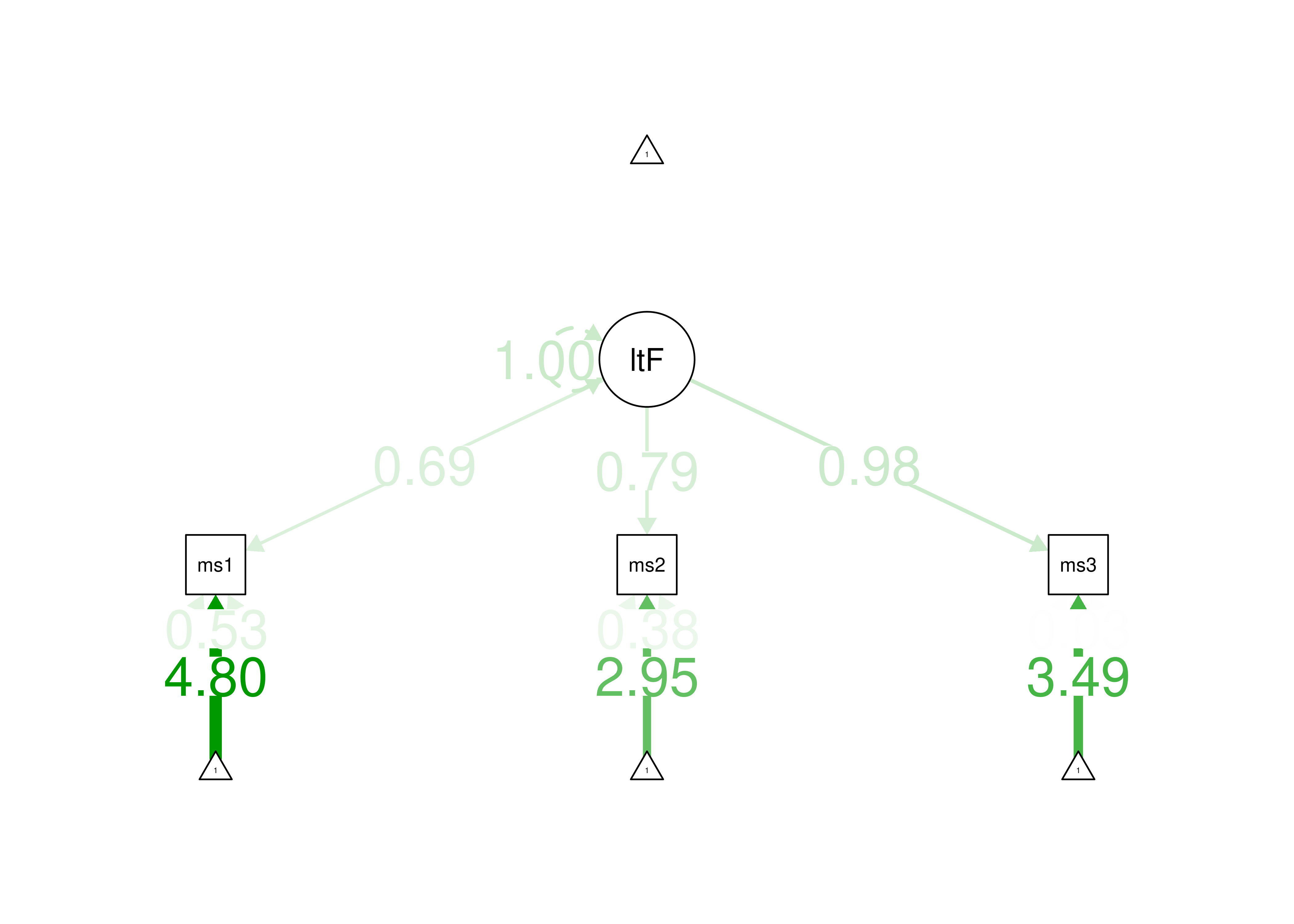
7.10 Confirmatory Factor Analysis (CFA)
The confirmatory factor analysis (CFA) models were fit in the lavaan package (Rosseel et al., 2022).
The examples were adapted from the lavaan documentation: https://lavaan.ugent.be/tutorial/cfa.html (archived at https://perma.cc/GKY3-9YE4).
In this CFA model, we estimate three latent factors with three indicators loading on each latent factor.
7.10.1 Specify the Model
Code
cfaModel_syntax <- '
 #Factor loadings
 visual  =~ x1 + x2 + x3
 textual =~ x4 + x5 + x6
 speed   =~ x7 + x8 + x9
'

cfaModel_fullSyntax <- '
 #Factor loadings (free the factor loading of the first indicator)
 visual  =~ NA*x1 + x2 + x3
 textual =~ NA*x4 + x5 + x6
 speed   =~ NA*x7 + x8 + x9

 #Fix latent means to zero
 visual ~ 0
 textual ~ 0
 speed ~ 0

 #Fix latent variances to one
 visual ~~ 1*visual
 textual ~~ 1*textual
 speed ~~ 1*speed

 #Estimate covariances among latent variables
 visual ~~ textual
 visual ~~ speed
 textual ~~ speed

 #Estimate residual variances of manifest variables
 x1 ~~ x1
 x2 ~~ x2
 x3 ~~ x3
 x4 ~~ x4
 x5 ~~ x5
 x6 ~~ x6
 x7 ~~ x7
 x8 ~~ x8
 x9 ~~ x9

 #Free intercepts of manifest variables
 x1 ~ int1*1
 x2 ~ int2*1
 x3 ~ int3*1
 x4 ~ int4*1
 x5 ~ int5*1
 x6 ~ int6*1
 x7 ~ int7*1
 x8 ~ int8*1
 x9 ~ int9*1
'7.10.3 Display Summary Output
In this model, all nine indicators load strongly on their respective latent factor. Thus, this measurement model would be defensible. In terms of interpretation, all indicators load positively on their respective latent factor, so higher levels of the latent factor are indicated by higher levels on the indicators.
lavaan 0.6-20 ended normally after 42 iterations

  Estimator                                         ML
  Optimization method                           NLMINB
  Number of model parameters                        30

  Number of observations                           301
  Number of missing patterns                         1

Model Test User Model:
                                              Standard      Scaled
  Test Statistic                                85.306      87.132
  Degrees of freedom                                24          24
  P-value (Chi-square)                           0.000       0.000
  Scaling correction factor                                  0.979
    Yuan-Bentler correction (Mplus variant)

Model Test Baseline Model:

  Test statistic                               918.852     880.082
  Degrees of freedom                                36          36
  P-value                                        0.000       0.000
  Scaling correction factor                                  1.044

User Model versus Baseline Model:

  Comparative Fit Index (CFI)                    0.931       0.925
  Tucker-Lewis Index (TLI)                       0.896       0.888

  Robust Comparative Fit Index (CFI)                         0.932
  Robust Tucker-Lewis Index (TLI)                            0.897

Loglikelihood and Information Criteria:

  Loglikelihood user model (H0)              -3737.745   -3737.745
  Scaling correction factor                                  1.093
      for the MLR correction
  Loglikelihood unrestricted model (H1)      -3695.092   -3695.092
  Scaling correction factor                                  1.043
      for the MLR correction

  Akaike (AIC)                                7535.490    7535.490
  Bayesian (BIC)                              7646.703    7646.703
  Sample-size adjusted Bayesian (SABIC)       7551.560    7551.560

Root Mean Square Error of Approximation:

  RMSEA                                          0.092       0.093
  90 Percent confidence interval - lower         0.071       0.073
  90 Percent confidence interval - upper         0.114       0.115
  P-value H_0: RMSEA <= 0.050                    0.001       0.001
  P-value H_0: RMSEA >= 0.080                    0.840       0.862

  Robust RMSEA                                               0.091
  90 Percent confidence interval - lower                     0.070
  90 Percent confidence interval - upper                     0.113
  P-value H_0: Robust RMSEA <= 0.050                         0.001
  P-value H_0: Robust RMSEA >= 0.080                         0.820

Standardized Root Mean Square Residual:

  SRMR                                           0.060       0.060

Parameter Estimates:

  Standard errors                             Sandwich
  Information bread                           Observed
  Observed information based on                Hessian

Latent Variables:
                   Estimate  Std.Err  z-value  P(>|z|)   Std.lv  Std.all
  visual =~
    x1                0.900    0.100    8.973    0.000    0.900    0.772
    x2                0.498    0.088    5.681    0.000    0.498    0.424
    x3                0.656    0.080    8.151    0.000    0.656    0.581
  textual =~
    x4                0.990    0.061   16.150    0.000    0.990    0.852
    x5                1.102    0.055   20.146    0.000    1.102    0.855
    x6                0.917    0.058   15.767    0.000    0.917    0.838
  speed =~
    x7                0.619    0.086    7.193    0.000    0.619    0.570
    x8                0.731    0.093    7.875    0.000    0.731    0.723
    x9                0.670    0.099    6.761    0.000    0.670    0.665

Covariances:
                   Estimate  Std.Err  z-value  P(>|z|)   Std.lv  Std.all
  visual ~~
    textual           0.459    0.073    6.258    0.000    0.459    0.459
    speed             0.471    0.119    3.954    0.000    0.471    0.471
  textual ~~
    speed             0.283    0.085    3.311    0.001    0.283    0.283

Intercepts:
                   Estimate  Std.Err  z-value  P(>|z|)   Std.lv  Std.all
   .x1                4.936    0.067   73.473    0.000    4.936    4.235
   .x2                6.088    0.068   89.855    0.000    6.088    5.179
   .x3                2.250    0.065   34.579    0.000    2.250    1.993
   .x4                3.061    0.067   45.694    0.000    3.061    2.634
   .x5                4.341    0.074   58.452    0.000    4.341    3.369
   .x6                2.186    0.063   34.667    0.000    2.186    1.998
   .x7                4.186    0.063   66.766    0.000    4.186    3.848
   .x8                5.527    0.058   94.854    0.000    5.527    5.467
   .x9                5.374    0.058   92.546    0.000    5.374    5.334

Variances:
                   Estimate  Std.Err  z-value  P(>|z|)   Std.lv  Std.all
   .x1                0.549    0.156    3.509    0.000    0.549    0.404
   .x2                1.134    0.112   10.135    0.000    1.134    0.821
   .x3                0.844    0.100    8.419    0.000    0.844    0.662
   .x4                0.371    0.050    7.382    0.000    0.371    0.275
   .x5                0.446    0.057    7.870    0.000    0.446    0.269
   .x6                0.356    0.047    7.658    0.000    0.356    0.298
   .x7                0.799    0.097    8.222    0.000    0.799    0.676
   .x8                0.488    0.120    4.080    0.000    0.488    0.477
   .x9                0.566    0.119    4.768    0.000    0.566    0.558
    visual            1.000                               1.000    1.000
    textual           1.000                               1.000    1.000
    speed             1.000                               1.000    1.000

R-Square:
                   Estimate
    x1                0.596
    x2                0.179
    x3                0.338
    x4                0.725
    x5                0.731
    x6                0.702
    x7                0.324
    x8                0.523
x9 0.442lavaan 0.6-20 ended normally after 42 iterations
Estimator ML
Optimization method NLMINB
Number of model parameters 30
Number of observations 301
Number of missing patterns 1
Model Test User Model:
Standard Scaled
Test Statistic 85.306 87.132
Degrees of freedom 24 24
P-value (Chi-square) 0.000 0.000
Scaling correction factor 0.979
Yuan-Bentler correction (Mplus variant)
Model Test Baseline Model:
Test statistic 918.852 880.082
Degrees of freedom 36 36
P-value 0.000 0.000
Scaling correction factor 1.044
User Model versus Baseline Model:
Comparative Fit Index (CFI) 0.931 0.925
Tucker-Lewis Index (TLI) 0.896 0.888
Robust Comparative Fit Index (CFI) 0.932
Robust Tucker-Lewis Index (TLI) 0.897
Loglikelihood and Information Criteria:
Loglikelihood user model (H0) -3737.745 -3737.745
Scaling correction factor 1.093
for the MLR correction
Loglikelihood unrestricted model (H1) -3695.092 -3695.092
Scaling correction factor 1.043
for the MLR correction
Akaike (AIC) 7535.490 7535.490
Bayesian (BIC) 7646.703 7646.703
Sample-size adjusted Bayesian (SABIC) 7551.560 7551.560
Root Mean Square Error of Approximation:
RMSEA 0.092 0.093
90 Percent confidence interval - lower 0.071 0.073
90 Percent confidence interval - upper 0.114 0.115
P-value H_0: RMSEA <= 0.050 0.001 0.001
P-value H_0: RMSEA >= 0.080 0.840 0.862
Robust RMSEA 0.091
90 Percent confidence interval - lower 0.070
90 Percent confidence interval - upper 0.113
P-value H_0: Robust RMSEA <= 0.050 0.001
P-value H_0: Robust RMSEA >= 0.080 0.820
Standardized Root Mean Square Residual:
SRMR 0.060 0.060
Parameter Estimates:
Standard errors Sandwich
Information bread Observed
Observed information based on Hessian
Latent Variables:
Estimate Std.Err z-value P(>|z|) Std.lv Std.all
visual =~
x1 0.900 0.100 8.973 0.000 0.900 0.772
x2 0.498 0.088 5.681 0.000 0.498 0.424
x3 0.656 0.080 8.151 0.000 0.656 0.581
textual =~
x4 0.990 0.061 16.150 0.000 0.990 0.852
x5 1.102 0.055 20.146 0.000 1.102 0.855
x6 0.917 0.058 15.767 0.000 0.917 0.838
speed =~
x7 0.619 0.086 7.193 0.000 0.619 0.570
x8 0.731 0.093 7.875 0.000 0.731 0.723
x9 0.670 0.099 6.761 0.000 0.670 0.665
Covariances:
Estimate Std.Err z-value P(>|z|) Std.lv Std.all
visual ~~
textual 0.459 0.073 6.258 0.000 0.459 0.459
speed 0.471 0.119 3.954 0.000 0.471 0.471
textual ~~
speed 0.283 0.085 3.311 0.001 0.283 0.283
Intercepts:
Estimate Std.Err z-value P(>|z|) Std.lv Std.all
visual 0.000 0.000 0.000
textual 0.000 0.000 0.000
speed 0.000 0.000 0.000
.x1 (int1) 4.936 0.067 73.473 0.000 4.936 4.235
.x2 (int2) 6.088 0.068 89.855 0.000 6.088 5.179
.x3 (int3) 2.250 0.065 34.579 0.000 2.250 1.993
.x4 (int4) 3.061 0.067 45.694 0.000 3.061 2.634
.x5 (int5) 4.341 0.074 58.452 0.000 4.341 3.369
.x6 (int6) 2.186 0.063 34.667 0.000 2.186 1.998
.x7 (int7) 4.186 0.063 66.766 0.000 4.186 3.848
.x8 (int8) 5.527 0.058 94.854 0.000 5.527 5.467
.x9 (int9) 5.374 0.058 92.546 0.000 5.374 5.334
Variances:
Estimate Std.Err z-value P(>|z|) Std.lv Std.all
visual 1.000 1.000 1.000
textual 1.000 1.000 1.000
speed 1.000 1.000 1.000
.x1 0.549 0.156 3.509 0.000 0.549 0.404
.x2 1.134 0.112 10.135 0.000 1.134 0.821
.x3 0.844 0.100 8.419 0.000 0.844 0.662
.x4 0.371 0.050 7.382 0.000 0.371 0.275
.x5 0.446 0.057 7.870 0.000 0.446 0.269
.x6 0.356 0.047 7.658 0.000 0.356 0.298
.x7 0.799 0.097 8.222 0.000 0.799 0.676
.x8 0.488 0.120 4.080 0.000 0.488 0.477
.x9 0.566 0.119 4.768 0.000 0.566 0.558
R-Square:
Estimate
x1 0.596
x2 0.179
x3 0.338
x4 0.725
x5 0.731
x6 0.702
x7 0.324
x8 0.523
x9 0.4427.10.4 Estimates of Model Fit
According to model fit estimates, the model fit is good according to SRMR and acceptable according to CFI, but the model fit is weaker according to RMSEA and TLI. Thus, we may want to consider adjustments to improve the model fit. In general, we want to make decisions regarding what parameters to estimate based on theory in conjunction with empiricism.
Code
               chisq                   df               pvalue
              85.306               24.000                0.000
        chisq.scaled            df.scaled        pvalue.scaled
              87.132               24.000                0.000
chisq.scaling.factor       baseline.chisq          baseline.df
               0.979              918.852               36.000
     baseline.pvalue                rmsea                  cfi
               0.000                0.092                0.931
                 tli                 srmr         rmsea.robust
               0.896                0.060                0.091
          cfi.robust           tli.robust
               0.932                0.897
7.10.5 Residuals
$type
[1] "cor.bollen"

$cov
       x1     x2     x3     x4     x5     x6     x7     x8     x9
x1  0.000
x2 -0.030  0.000
x3 -0.008  0.094  0.000
x4  0.071 -0.012 -0.068  0.000
x5 -0.009 -0.027 -0.151  0.005  0.000
x6  0.060  0.030 -0.026 -0.009  0.003  0.000
x7 -0.140 -0.189 -0.084  0.037 -0.036 -0.014  0.000
x8 -0.039 -0.052 -0.012 -0.067 -0.036 -0.022  0.075  0.000
x9  0.149  0.073  0.147  0.048  0.067  0.056 -0.038 -0.032  0.000

$mean
x1 x2 x3 x4 x5 x6 x7 x8 x9
 0  0  0  0  0  0  0  0  0
7.10.6 Modification Indices
Modification indices indicate potential additional parameters that could be estimated and that would improve model fit. For instance, the modification indices in Table ?? (generated from the syntax below) indicate a few additional factor loadings (i.e., cross-loadings) or correlated residuals that could substantially improve model fit. However, it is generally not recommended to blindly estimate additional parameters solely based on modification indices. Rather, it is generally advised to consider modification indices in light of theory.
7.10.8 Internal Consistency Reliability
Internal consistency reliability of items composing the latent factors, as quantified by omega (\(\omega\)) and average variance extracted (AVE), was estimated using the semTools package (Jorgensen et al., 2021).
 visual textual   speed
0.612 0.885 0.686 visual textual speed
0.371 0.721 0.424 7.10.9 Path Diagram
Below is a path diagram of the model generated using the semPlot package (Epskamp, 2022).
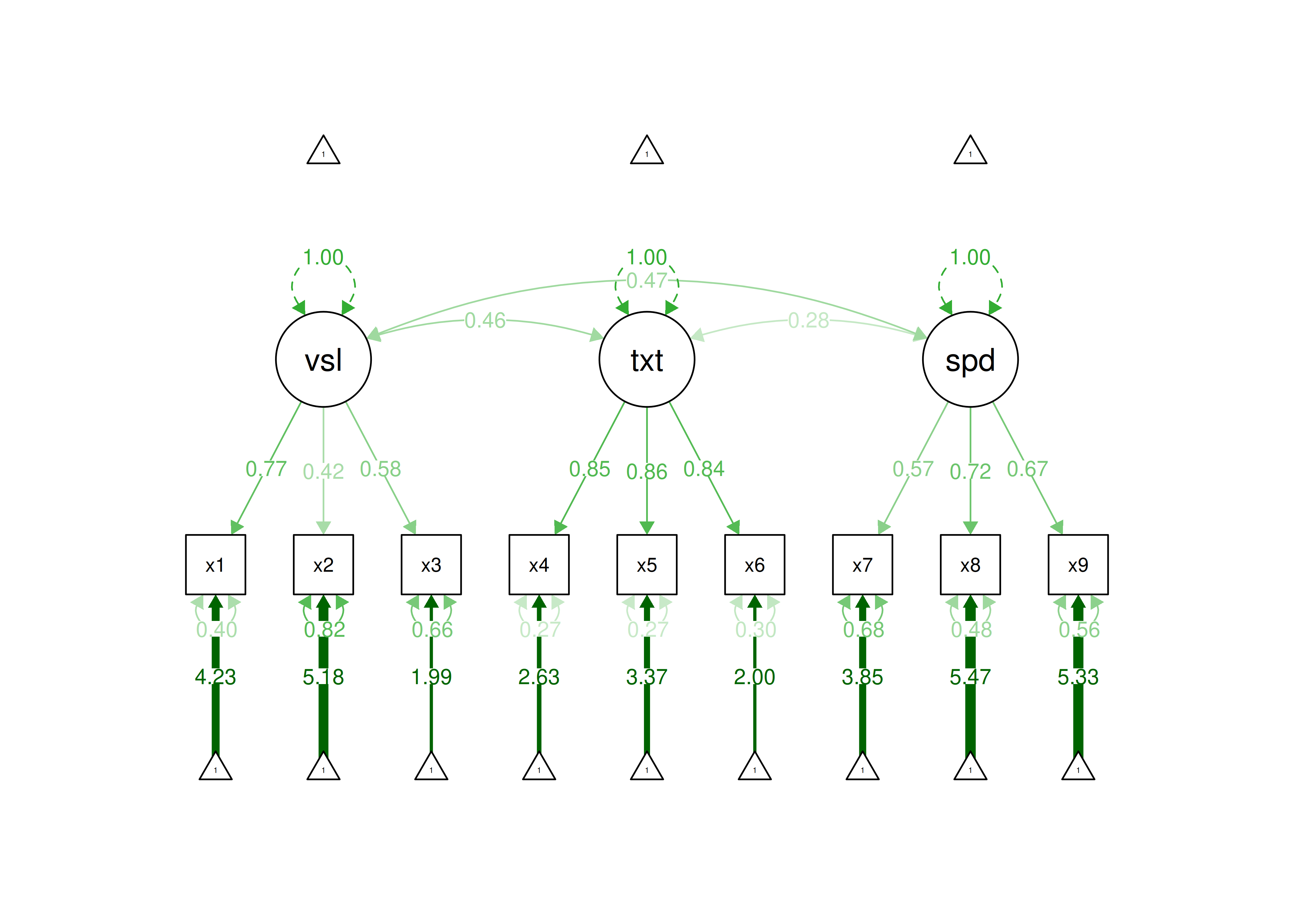
Figure 7.9: Confirmatory Factor Analysis Model.
7.10.10 Modify Model Based on Modification Indices
In the model below, I modified the model based on estimating an additional factor loading (assuming the additional factor loading is theoretically supported). This could be supported, for instance, if a given test involves considerable skills in both the visual domain and in speed of processing. When the same indicator loads simultaneously on two factors, this is called a cross-loading. Cross-loadings can complicate the interpretation of latent factors, as discussed in Section 14.1.4.5 of the chapter on factor analysis.
7.10.10.1 Specify the Model
Code
cfaModel2_syntax <- '
 #Factor loadings
 textual =~ x4 + x5 + x6
 visual  =~ x1 + x2 + x3 + x9
 speed   =~ x7 + x8 + x9
'

cfaModel2_fullSyntax <- '
 #Factor loadings (free the factor loading of the first indicator)
 textual =~ NA*x4 + x5 + x6
 visual  =~ NA*x1 + x2 + x3 + x9
 speed   =~ NA*x7 + x8 + x9

 #Fix latent means to zero
 visual ~ 0
 textual ~ 0
 speed ~ 0

 #Fix latent variances to one
 visual ~~ 1*visual
 textual ~~ 1*textual
 speed ~~ 1*speed

 #Estimate covariances among latent variables
 visual ~~ textual
 visual ~~ speed
 textual ~~ speed

 #Estimate residual variances of manifest variables
 x1 ~~ x1
 x2 ~~ x2
 x3 ~~ x3
 x4 ~~ x4
 x5 ~~ x5
 x6 ~~ x6
 x7 ~~ x7
 x8 ~~ x8
 x9 ~~ x9

 #Free intercepts of manifest variables
 x1 ~ int1*1
 x2 ~ int2*1
 x3 ~ int3*1
 x4 ~ int4*1
 x5 ~ int5*1
 x6 ~ int6*1
 x7 ~ int7*1
 x8 ~ int8*1
 x9 ~ int9*1
'7.10.10.3 Display Summary Output
lavaan 0.6-20 ended normally after 39 iterations

  Estimator                                         ML
  Optimization method                           NLMINB
  Number of model parameters                        31

  Number of observations                           301
  Number of missing patterns                         1

Model Test User Model:
                                              Standard      Scaled
  Test Statistic                                52.382      51.725
  Degrees of freedom                                23          23
  P-value (Chi-square)                           0.000       0.001
  Scaling correction factor                                  1.013
    Yuan-Bentler correction (Mplus variant)

Model Test Baseline Model:

  Test statistic                               918.852     880.082
  Degrees of freedom                                36          36
  P-value                                        0.000       0.000
  Scaling correction factor                                  1.044

User Model versus Baseline Model:

  Comparative Fit Index (CFI)                    0.967       0.966
  Tucker-Lewis Index (TLI)                       0.948       0.947

  Robust Comparative Fit Index (CFI)                         0.968
  Robust Tucker-Lewis Index (TLI)                            0.950

Loglikelihood and Information Criteria:

  Loglikelihood user model (H0)              -3721.283   -3721.283
  Scaling correction factor                                  1.065
      for the MLR correction
  Loglikelihood unrestricted model (H1)      -3695.092   -3695.092
  Scaling correction factor                                  1.043
      for the MLR correction

  Akaike (AIC)                                7504.566    7504.566
  Bayesian (BIC)                              7619.487    7619.487
  Sample-size adjusted Bayesian (SABIC)       7521.172    7521.172

Root Mean Square Error of Approximation:

  RMSEA                                          0.065       0.064
  90 Percent confidence interval - lower         0.042       0.041
  90 Percent confidence interval - upper         0.089       0.088
  P-value H_0: RMSEA <= 0.050                    0.133       0.143
  P-value H_0: RMSEA >= 0.080                    0.158       0.144

  Robust RMSEA                                               0.064
  90 Percent confidence interval - lower                     0.040
  90 Percent confidence interval - upper                     0.088
  P-value H_0: Robust RMSEA <= 0.050                         0.156
  P-value H_0: Robust RMSEA >= 0.080                         0.147

Standardized Root Mean Square Residual:

  SRMR                                           0.041       0.041

Parameter Estimates:

  Standard errors                             Sandwich
  Information bread                           Observed
  Observed information based on                Hessian

Latent Variables:
                   Estimate  Std.Err  z-value  P(>|z|)   Std.lv  Std.all
  textual =~
    x4                0.989    0.061   16.150    0.000    0.989    0.851
    x5                1.103    0.055   20.196    0.000    1.103    0.856
    x6                0.916    0.058   15.728    0.000    0.916    0.838
  visual =~
    x1                0.885    0.091    9.673    0.000    0.885    0.759
    x2                0.511    0.082    6.233    0.000    0.511    0.435
    x3                0.667    0.072    9.214    0.000    0.667    0.590
    x9                0.387    0.066    5.895    0.000    0.387    0.384
  speed =~
    x7                0.666    0.075    8.874    0.000    0.666    0.612
    x8                0.804    0.080    9.997    0.000    0.804    0.795
    x9                0.450    0.065    6.901    0.000    0.450    0.447

Covariances:
                   Estimate  Std.Err  z-value  P(>|z|)   Std.lv  Std.all
  textual ~~
    visual            0.453    0.074    6.091    0.000    0.453    0.453
    speed             0.206    0.076    2.731    0.006    0.206    0.206
  visual ~~
    speed             0.301    0.084    3.567    0.000    0.301    0.301

Intercepts:
                   Estimate  Std.Err  z-value  P(>|z|)   Std.lv  Std.all
   .x4                3.061    0.067   45.694    0.000    3.061    2.634
   .x5                4.341    0.074   58.452    0.000    4.341    3.369
   .x6                2.186    0.063   34.667    0.000    2.186    1.998
   .x1                4.936    0.067   73.473    0.000    4.936    4.235
   .x2                6.088    0.068   89.855    0.000    6.088    5.179
   .x3                2.250    0.065   34.579    0.000    2.250    1.993
   .x9                5.374    0.058   92.546    0.000    5.374    5.334
   .x7                4.186    0.063   66.766    0.000    4.186    3.848
   .x8                5.527    0.058   94.854    0.000    5.527    5.467

Variances:
                   Estimate  Std.Err  z-value  P(>|z|)   Std.lv  Std.all
   .x4                0.373    0.050    7.403    0.000    0.373    0.276
   .x5                0.444    0.057    7.827    0.000    0.444    0.267
   .x6                0.357    0.046    7.674    0.000    0.357    0.298
   .x1                0.576    0.135    4.256    0.000    0.576    0.424
   .x2                1.120    0.109   10.296    0.000    1.120    0.811
   .x3                0.830    0.087    9.561    0.000    0.830    0.651
   .x9                0.558    0.066    8.482    0.000    0.558    0.550
   .x7                0.740    0.089    8.266    0.000    0.740    0.625
   .x8                0.375    0.105    3.583    0.000    0.375    0.367
    textual           1.000                               1.000    1.000
    visual            1.000                               1.000    1.000
    speed             1.000                               1.000    1.000

R-Square:
                   Estimate
    x4                0.724
    x5                0.733
    x6                0.702
    x1                0.576
    x2                0.189
    x3                0.349
    x9                0.450
    x7                0.375
x8 0.633lavaan 0.6-20 ended normally after 39 iterations
Estimator ML
Optimization method NLMINB
Number of model parameters 31
Number of observations 301
Number of missing patterns 1
Model Test User Model:
Standard Scaled
Test Statistic 52.382 51.725
Degrees of freedom 23 23
P-value (Chi-square) 0.000 0.001
Scaling correction factor 1.013
Yuan-Bentler correction (Mplus variant)
Model Test Baseline Model:
Test statistic 918.852 880.082
Degrees of freedom 36 36
P-value 0.000 0.000
Scaling correction factor 1.044
User Model versus Baseline Model:
Comparative Fit Index (CFI) 0.967 0.966
Tucker-Lewis Index (TLI) 0.948 0.947
Robust Comparative Fit Index (CFI) 0.968
Robust Tucker-Lewis Index (TLI) 0.950
Loglikelihood and Information Criteria:
Loglikelihood user model (H0) -3721.283 -3721.283
Scaling correction factor 1.065
for the MLR correction
Loglikelihood unrestricted model (H1) -3695.092 -3695.092
Scaling correction factor 1.043
for the MLR correction
Akaike (AIC) 7504.566 7504.566
Bayesian (BIC) 7619.487 7619.487
Sample-size adjusted Bayesian (SABIC) 7521.172 7521.172
Root Mean Square Error of Approximation:
RMSEA 0.065 0.064
90 Percent confidence interval - lower 0.042 0.041
90 Percent confidence interval - upper 0.089 0.088
P-value H_0: RMSEA <= 0.050 0.133 0.143
P-value H_0: RMSEA >= 0.080 0.158 0.144
Robust RMSEA 0.064
90 Percent confidence interval - lower 0.040
90 Percent confidence interval - upper 0.088
P-value H_0: Robust RMSEA <= 0.050 0.156
P-value H_0: Robust RMSEA >= 0.080 0.147
Standardized Root Mean Square Residual:
SRMR 0.041 0.041
Parameter Estimates:
Standard errors Sandwich
Information bread Observed
Observed information based on Hessian
Latent Variables:
Estimate Std.Err z-value P(>|z|) Std.lv Std.all
textual =~
x4 0.989 0.061 16.150 0.000 0.989 0.851
x5 1.103 0.055 20.196 0.000 1.103 0.856
x6 0.916 0.058 15.728 0.000 0.916 0.838
visual =~
x1 0.885 0.091 9.673 0.000 0.885 0.759
x2 0.511 0.082 6.233 0.000 0.511 0.435
x3 0.667 0.072 9.214 0.000 0.667 0.590
x9 0.387 0.066 5.895 0.000 0.387 0.384
speed =~
x7 0.666 0.075 8.874 0.000 0.666 0.612
x8 0.804 0.080 9.997 0.000 0.804 0.795
x9 0.450 0.065 6.901 0.000 0.450 0.447
Covariances:
Estimate Std.Err z-value P(>|z|) Std.lv Std.all
textual ~~
visual 0.453 0.074 6.091 0.000 0.453 0.453
visual ~~
speed 0.301 0.084 3.567 0.000 0.301 0.301
textual ~~
speed 0.206 0.076 2.731 0.006 0.206 0.206
Intercepts:
Estimate Std.Err z-value P(>|z|) Std.lv Std.all
visual 0.000 0.000 0.000
textual 0.000 0.000 0.000
speed 0.000 0.000 0.000
.x1 (int1) 4.936 0.067 73.473 0.000 4.936 4.235
.x2 (int2) 6.088 0.068 89.855 0.000 6.088 5.179
.x3 (int3) 2.250 0.065 34.579 0.000 2.250 1.993
.x4 (int4) 3.061 0.067 45.694 0.000 3.061 2.634
.x5 (int5) 4.341 0.074 58.452 0.000 4.341 3.369
.x6 (int6) 2.186 0.063 34.667 0.000 2.186 1.998
.x7 (int7) 4.186 0.063 66.766 0.000 4.186 3.848
.x8 (int8) 5.527 0.058 94.854 0.000 5.527 5.467
.x9 (int9) 5.374 0.058 92.546 0.000 5.374 5.334
Variances:
Estimate Std.Err z-value P(>|z|) Std.lv Std.all
visual 1.000 1.000 1.000
textual 1.000 1.000 1.000
speed 1.000 1.000 1.000
.x1 0.576 0.135 4.256 0.000 0.576 0.424
.x2 1.120 0.109 10.296 0.000 1.120 0.811
.x3 0.830 0.087 9.561 0.000 0.830 0.651
.x4 0.373 0.050 7.403 0.000 0.373 0.276
.x5 0.444 0.057 7.827 0.000 0.444 0.267
.x6 0.357 0.046 7.674 0.000 0.357 0.298
.x7 0.740 0.089 8.266 0.000 0.740 0.625
.x8 0.375 0.105 3.583 0.000 0.375 0.367
.x9 0.558 0.066 8.482 0.000 0.558 0.550
R-Square:
Estimate
x1 0.576
x2 0.189
x3 0.349
x4 0.724
x5 0.733
x6 0.702
x7 0.375
x8 0.633
x9 0.4507.10.10.4 Estimates of Model Fit
After fitting the additional factor loading, the model fits well according to RMSEA, CFI, and SRMR, and the model fit is acceptable according to TLI. Thus, this model could be defensible.
Code
               chisq                   df               pvalue
              52.382               23.000                0.000
        chisq.scaled            df.scaled        pvalue.scaled
              51.725               23.000                0.001
chisq.scaling.factor       baseline.chisq          baseline.df
               1.013              918.852               36.000
     baseline.pvalue                rmsea                  cfi
               0.000                0.065                0.967
                 tli                 srmr         rmsea.robust
               0.948                0.041                0.064
          cfi.robust           tli.robust
               0.968                0.950
7.10.10.5 Residuals
$type
[1] "cor.bollen"

$cov
       x4     x5     x6     x1     x2     x3     x9     x7     x8
x4  0.000
x5  0.005  0.000
x6 -0.008  0.003  0.000
x1  0.080 -0.001  0.069  0.000
x2 -0.015 -0.029  0.028 -0.033  0.000
x3 -0.069 -0.152 -0.026 -0.008  0.083  0.000
x9 -0.018  0.000 -0.009 -0.003 -0.019  0.023  0.000
x7  0.066 -0.006  0.015 -0.073 -0.156 -0.037 -0.003  0.000
x8 -0.033 -0.002  0.012  0.042 -0.012  0.045  0.002  0.000  0.000

$mean
x4 x5 x6 x1 x2 x3 x9 x7 x8
 0  0  0  0  0  0  0  0  0
7.10.10.6 Path Diagram
Below is a path diagram of the model generated using the semPlot package (Epskamp, 2022).
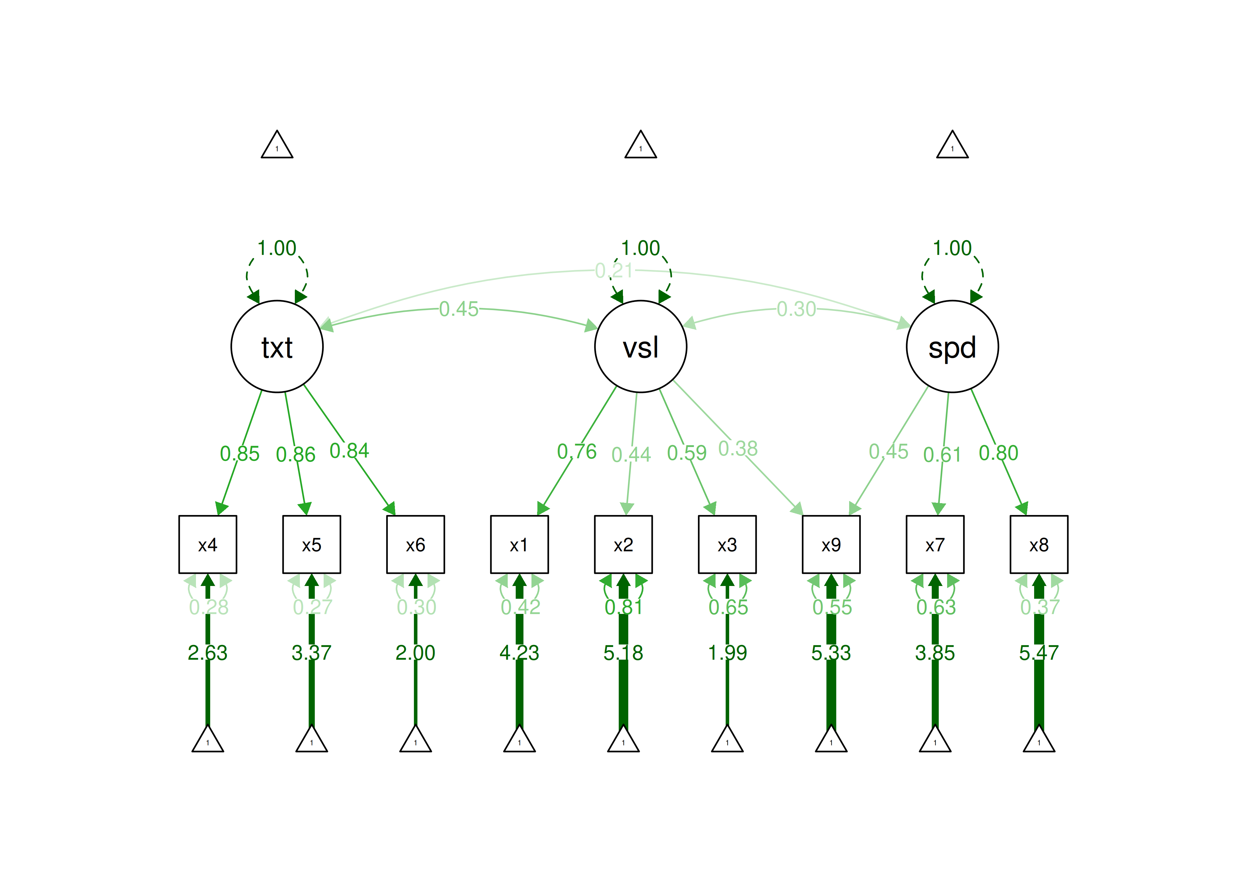
Figure 7.10: Modified Confirmatory Factor Analysis Model.
7.10.10.7 Compare Model Fit
The modified model with the cross-loading and the original model are considered “nested” models.
The original model is nested within the modified model because the modified model includes all of the terms of the original model along with additional terms.
To confirm that the models are nested, I use the net() function from the semTools package (Jorgensen et al., 2021).
        If cell [R, C] is TRUE, the model in row R is nested within column C.

        If the models also have the same degrees of freedom, they are equivalent.

        NA indicates the model in column C did not converge when fit to the
        implied means and covariance matrix from the model in row R.

        The hidden diagonal is TRUE because any model is equivalent to itself.
        The upper triangle is hidden because for models with the same degrees
        of freedom, cell [C, R] == cell [R, C].  For all models with different
        degrees of freedom, the upper diagonal is all FALSE because models with
        fewer degrees of freedom (i.e., more parameters) cannot be nested
        within models with more degrees of freedom (i.e., fewer parameters).

                       cfaModel2Fit cfaModelFit
cfaModel2Fit (df = 23)
cfaModelFit (df = 24)  TRUE
Model fit of nested models can be compared with a chi-square difference test.
In this case, the model with the cross-loading fits significantly better (i.e., has a significantly smaller chi-square value) than the model without the cross-loading.
One can also compare nested models using a robust likelihood ratio test:
Code
Model 1
 Class: lavaan
 Call: lavaan::lavaan(model = cfaModel2_syntax, data = HolzingerSwineford1939, ...

Model 2
 Class: lavaan
 Call: lavaan::lavaan(model = cfaModel_syntax, data = HolzingerSwineford1939, ...

Variance test
  H0: Model 1 and Model 2 are indistinguishable
  H1: Model 1 and Model 2 are distinguishable
    w2 = 0.120,   p = 0.00049

Robust likelihood ratio test of distinguishable models
  H0: Model 2 fits as well as Model 1
  H1: Model 1 fits better than Model 2
    LR = 32.923,   p = 8.11e-08
For non-nested models, one can compare model fit with AIC, BIC, or the Vuong test.
     aic      bic     bic2
7535.490 7646.703 7551.560 aic bic bic2
7504.566 7619.487 7521.172
Model 1
 Class: lavaan
 Call: lavaan::lavaan(model = cfaModel_syntax, data = HolzingerSwineford1939, ...

Model 2
 Class: lavaan
 Call: lavaan::lavaan(model = cfaModel2_syntax, data = HolzingerSwineford1939, ...

Variance test
  H0: Model 1 and Model 2 are indistinguishable
  H1: Model 1 and Model 2 are distinguishable
    w2 = 0.120,   p = 0.00049

Non-nested likelihood ratio test
  H0: Model fits are equal for the focal population
  H1A: Model 1 fits better than Model 2
    z = -2.734,   p = 0.997
  H1B: Model 2 fits better than Model 1
    z = -2.734,   p = 0.003128
7.11 Structural Equation Model (SEM)
The structural equation models were fit in the lavaan package (Rosseel et al., 2022).
The examples were adapted from the lavaan documentation: https://lavaan.ugent.be/tutorial/sem.html (archived at https://perma.cc/8NG9-7JAG).
In this model, we fit a measurement model with three latent factors in addition to a structural model with regressions estimated among the latent factors.
7.11.1 Specify the Model
Code
semModel_syntax <- '
 #Measurement model factor loadings
 ind60 =~ x1 + x2 + x3
 dem60 =~ y1 + y2 + y3 + y4
 dem65 =~ y5 + y6 + y7 + y8

 #Regression paths
 dem60 ~ ind60
 dem65 ~ ind60 + dem60

 #Covariances among residual variances (correlated errors)
 y1 ~~ y5
 y2 ~~ y4 + y6
 y3 ~~ y7
 y4 ~~ y8
 y6 ~~ y8
'

semModel_fullSyntax <- '
 #Measurement model factor loadings (free the factor loading of the first indicator)
 ind60 =~ NA*x1 + x2 + x3
 dem60 =~ NA*y1 + y2 + y3 + y4
 dem65 =~ NA*y5 + y6 + y7 + y8

 #Regression paths
 dem60 ~ ind60
 dem65 ~ ind60 + dem60

 #Covariances among residual variances (correlated errors)
 y1 ~~ y5
 y2 ~~ y4 + y6
 y3 ~~ y7
 y4 ~~ y8
 y6 ~~ y8

 #Fix latent means to zero
 ind60 ~ 0
 dem60 ~ 0
 dem65 ~ 0

 #Fix latent variances to one
 ind60 ~~ 1*ind60
 dem60 ~~ 1*dem60
 dem65 ~~ 1*dem65

 #Estimate covariances among latent variables (not necessary because the latent variables are already linked via regression paths)

 #Estimate residual variances of manifest variables
 x1 ~~ x1
 x2 ~~ x2
 x3 ~~ x3
 y1 ~~ y1
 y2 ~~ y2
 y3 ~~ y3
 y4 ~~ y4
 y5 ~~ y5
 y6 ~~ y6
 y7 ~~ y7
 y8 ~~ y8

 #Free intercepts of manifest variables
 x1 ~ intx1*1
 x2 ~ intx2*1
 x3 ~ intx3*1
 y1 ~ inty1*1
 y2 ~ inty2*1
 y3 ~ inty3*1
 y4 ~ inty4*1
 y5 ~ inty5*1
 y6 ~ inty6*1
 y7 ~ inty7*1
 y8 ~ inty8*1
'7.11.3 Display Summary Output
7.11.3.1 Interpreting lavaan Output
Output from a SEM model includes information such as regression coefficients, intercepts, variances, and model fit indices.
As noted above, there are two chi-square tests.
In lavaan syntax, one is labeled “Model Test User Model” and the other is labeled “Model Test Baseline Model.”
The chi-square test labeled “Model Test User Model” refers to the chi-square test of whether the model fits worse than the best-possible fitting model (the saturated model).
In this case, the p-value of the robust chi-square test is \(0.17\).
Thus, the model does not show significant misfit—i.e., the model does not fit significantly worse than the best-possible fitting model.
The chi-square test labeled “Model Test Baseline Model” refers to the chi-square test of whether the model fits better than the worst-possible fitting model (the null model).
In this case, the p-value of the robust chi-square test in comparison to the worse-possible fitting model is < .05.
Thus, the model fits significantly better than the worst-possible-fitting model.
In terms of the model findings, ind60 was significantly positively associated with dem60, dem60 was significantly positively associated with dem65, and ind60 was marginally significantly positively associated with dem65.
lavaan 0.6-20 ended normally after 82 iterations

  Estimator                                         ML
  Optimization method                           NLMINB
  Number of model parameters                        42

  Number of observations                            75
  Number of missing patterns                        36

Model Test User Model:
                                              Standard      Scaled
  Test Statistic                                38.748      42.709
  Degrees of freedom                                35          35
  P-value (Chi-square)                           0.304       0.174
  Scaling correction factor                                  0.907
    Yuan-Bentler correction (Mplus variant)

Model Test Baseline Model:

  Test statistic                               601.314     594.441
  Degrees of freedom                                55          55
  P-value                                        0.000       0.000
  Scaling correction factor                                  1.012

User Model versus Baseline Model:

  Comparative Fit Index (CFI)                    0.993       0.986
  Tucker-Lewis Index (TLI)                       0.989       0.978

  Robust Comparative Fit Index (CFI)                         0.988
  Robust Tucker-Lewis Index (TLI)                            0.981

Loglikelihood and Information Criteria:

  Loglikelihood user model (H0)              -1418.424   -1418.424
  Scaling correction factor                                  0.989
      for the MLR correction
  Loglikelihood unrestricted model (H1)      -1399.050   -1399.050
  Scaling correction factor                                  0.952
      for the MLR correction

  Akaike (AIC)                                2920.848    2920.848
  Bayesian (BIC)                              3018.183    3018.183
  Sample-size adjusted Bayesian (SABIC)       2885.810    2885.810

Root Mean Square Error of Approximation:

  RMSEA                                          0.038       0.054
  90 Percent confidence interval - lower         0.000       0.000
  90 Percent confidence interval - upper         0.094       0.106
  P-value H_0: RMSEA <= 0.050                    0.585       0.424
  P-value H_0: RMSEA >= 0.080                    0.126       0.240

  Robust RMSEA                                               0.055
  90 Percent confidence interval - lower                     0.000
  90 Percent confidence interval - upper                     0.113
  P-value H_0: Robust RMSEA <= 0.050                         0.422
  P-value H_0: Robust RMSEA >= 0.080                         0.279

Standardized Root Mean Square Residual:

  SRMR                                           0.046       0.046

Parameter Estimates:

  Standard errors                             Sandwich
  Information bread                           Observed
  Observed information based on                Hessian

Latent Variables:
                   Estimate  Std.Err  z-value  P(>|z|)   Std.lv  Std.all
  ind60 =~
    x1                0.645    0.056   11.566    0.000    0.645    0.908
    x2                1.495    0.124   12.084    0.000    1.495    0.991
    x3                1.189    0.112   10.581    0.000    1.189    0.863
  dem60 =~
    y1                1.879    0.239    7.858    0.000    2.143    0.834
    y2                2.477    0.308    8.043    0.000    2.825    0.714
    y3                2.134    0.330    6.469    0.000    2.434    0.733
    y4                2.523    0.254    9.918    0.000    2.879    0.864
  dem65 =~
    y5                0.547    0.228    2.398    0.016    2.090    0.791
    y6                0.656    0.275    2.390    0.017    2.509    0.753
    y7                0.715    0.315    2.265    0.024    2.732    0.830
    y8                0.696    0.311    2.240    0.025    2.660    0.805

Regressions:
                   Estimate  Std.Err  z-value  P(>|z|)   Std.lv  Std.all
  dem60 ~
    ind60             0.549    0.162    3.381    0.001    0.481    0.481
  dem65 ~
    ind60             0.690    0.391    1.766    0.077    0.180    0.180
    dem60             2.900    1.362    2.129    0.033    0.865    0.865

Covariances:
                   Estimate  Std.Err  z-value  P(>|z|)   Std.lv  Std.all
 .y1 ~~
   .y5                0.728    0.511    1.427    0.154    0.728    0.318
 .y2 ~~
   .y4                1.087    0.847    1.284    0.199    1.087    0.234
   .y6                1.672    0.957    1.747    0.081    1.672    0.275
 .y3 ~~
   .y7                0.343    0.750    0.457    0.647    0.343    0.083
 .y4 ~~
   .y8                0.501    0.457    1.097    0.273    0.501    0.153
 .y6 ~~
   .y8                1.720    0.843    2.040    0.041    1.720    0.400

Intercepts:
                   Estimate  Std.Err  z-value  P(>|z|)   Std.lv  Std.all
   .x1                5.064    0.084   60.554    0.000    5.064    7.131
   .x2                4.829    0.176   27.401    0.000    4.829    3.202
   .x3                3.524    0.163   21.557    0.000    3.524    2.557
   .y1                5.512    0.300   18.389    0.000    5.512    2.145
   .y2                4.273    0.468    9.127    0.000    4.273    1.080
   .y3                6.558    0.385   17.026    0.000    6.558    1.974
   .y4                4.391    0.392   11.214    0.000    4.391    1.319
   .y5                5.132    0.312   16.434    0.000    5.132    1.942
   .y6                2.979    0.390    7.642    0.000    2.979    0.894
   .y7                6.310    0.387   16.315    0.000    6.310    1.918
   .y8                4.019    0.392   10.247    0.000    4.019    1.217

Variances:
                   Estimate  Std.Err  z-value  P(>|z|)   Std.lv  Std.all
   .x1                0.088    0.023    3.792    0.000    0.088    0.175
   .x2                0.040    0.097    0.410    0.682    0.040    0.017
   .x3                0.486    0.090    5.418    0.000    0.486    0.256
   .y1                2.009    0.506    3.973    0.000    2.009    0.304
   .y2                7.675    1.433    5.354    0.000    7.675    0.490
   .y3                5.116    1.157    4.420    0.000    5.116    0.463
   .y4                2.803    0.883    3.175    0.001    2.803    0.253
   .y5                2.618    0.686    3.815    0.000    2.618    0.375
   .y6                4.819    0.987    4.884    0.000    4.819    0.434
   .y7                3.362    0.714    4.709    0.000    3.362    0.311
   .y8                3.835    1.001    3.831    0.000    3.835    0.352
    ind60             1.000                               1.000    1.000
   .dem60             1.000                               0.768    0.768
   .dem65             1.000                               0.068    0.068

R-Square:
                   Estimate
    x1                0.825
    x2                0.983
    x3                0.744
    y1                0.696
    y2                0.510
    y3                0.537
    y4                0.747
    y5                0.625
    y6                0.566
    y7                0.689
    y8                0.648
    dem60             0.232
dem65 0.932lavaan 0.6-20 ended normally after 82 iterations
Estimator ML
Optimization method NLMINB
Number of model parameters 42
Number of observations 75
Number of missing patterns 36
Model Test User Model:
Standard Scaled
Test Statistic 38.748 42.709
Degrees of freedom 35 35
P-value (Chi-square) 0.304 0.174
Scaling correction factor 0.907
Yuan-Bentler correction (Mplus variant)
Model Test Baseline Model:
Test statistic 601.314 594.441
Degrees of freedom 55 55
P-value 0.000 0.000
Scaling correction factor 1.012
User Model versus Baseline Model:
Comparative Fit Index (CFI) 0.993 0.986
Tucker-Lewis Index (TLI) 0.989 0.978
Robust Comparative Fit Index (CFI) 0.988
Robust Tucker-Lewis Index (TLI) 0.981
Loglikelihood and Information Criteria:
Loglikelihood user model (H0) -1418.424 -1418.424
Scaling correction factor 0.989
for the MLR correction
Loglikelihood unrestricted model (H1) -1399.050 -1399.050
Scaling correction factor 0.952
for the MLR correction
Akaike (AIC) 2920.848 2920.848
Bayesian (BIC) 3018.183 3018.183
Sample-size adjusted Bayesian (SABIC) 2885.810 2885.810
Root Mean Square Error of Approximation:
RMSEA 0.038 0.054
90 Percent confidence interval - lower 0.000 0.000
90 Percent confidence interval - upper 0.094 0.106
P-value H_0: RMSEA <= 0.050 0.585 0.424
P-value H_0: RMSEA >= 0.080 0.126 0.240
Robust RMSEA 0.055
90 Percent confidence interval - lower 0.000
90 Percent confidence interval - upper 0.113
P-value H_0: Robust RMSEA <= 0.050 0.422
P-value H_0: Robust RMSEA >= 0.080 0.279
Standardized Root Mean Square Residual:
SRMR 0.046 0.046
Parameter Estimates:
Standard errors Sandwich
Information bread Observed
Observed information based on Hessian
Latent Variables:
Estimate Std.Err z-value P(>|z|) Std.lv Std.all
ind60 =~
x1 0.645 0.056 11.566 0.000 0.645 0.908
x2 1.495 0.124 12.084 0.000 1.495 0.991
x3 1.189 0.112 10.581 0.000 1.189 0.863
dem60 =~
y1 1.879 0.239 7.858 0.000 2.143 0.834
y2 2.477 0.308 8.043 0.000 2.825 0.714
y3 2.134 0.330 6.469 0.000 2.434 0.733
y4 2.523 0.254 9.918 0.000 2.879 0.864
dem65 =~
y5 0.547 0.228 2.398 0.016 2.090 0.791
y6 0.656 0.275 2.390 0.017 2.509 0.753
y7 0.715 0.315 2.265 0.024 2.732 0.830
y8 0.696 0.311 2.240 0.025 2.660 0.805
Regressions:
Estimate Std.Err z-value P(>|z|) Std.lv Std.all
dem60 ~
ind60 0.549 0.162 3.381 0.001 0.481 0.481
dem65 ~
ind60 0.690 0.391 1.766 0.077 0.180 0.180
dem60 2.900 1.362 2.129 0.033 0.865 0.865
Covariances:
Estimate Std.Err z-value P(>|z|) Std.lv Std.all
.y1 ~~
.y5 0.728 0.511 1.427 0.154 0.728 0.318
.y2 ~~
.y4 1.087 0.847 1.284 0.199 1.087 0.234
.y6 1.672 0.957 1.747 0.081 1.672 0.275
.y3 ~~
.y7 0.343 0.750 0.457 0.647 0.343 0.083
.y4 ~~
.y8 0.501 0.457 1.097 0.273 0.501 0.153
.y6 ~~
.y8 1.720 0.843 2.040 0.041 1.720 0.400
Intercepts:
Estimate Std.Err z-value P(>|z|) Std.lv Std.all
ind60 0.000 0.000 0.000
.dem60 0.000 0.000 0.000
.dem65 0.000 0.000 0.000
.x1 (intx1) 5.064 0.084 60.554 0.000 5.064 7.131
.x2 (intx2) 4.829 0.176 27.401 0.000 4.829 3.202
.x3 (intx3) 3.524 0.163 21.557 0.000 3.524 2.557
.y1 (inty1) 5.512 0.300 18.389 0.000 5.512 2.145
.y2 (inty2) 4.273 0.468 9.127 0.000 4.273 1.080
.y3 (inty3) 6.558 0.385 17.026 0.000 6.558 1.974
.y4 (int4) 4.391 0.392 11.214 0.000 4.391 1.319
.y5 (int5) 5.132 0.312 16.434 0.000 5.132 1.942
.y6 (int6) 2.979 0.390 7.642 0.000 2.979 0.894
.y7 (int7) 6.310 0.387 16.315 0.000 6.310 1.918
.y8 (int8) 4.019 0.392 10.247 0.000 4.019 1.217
Variances:
Estimate Std.Err z-value P(>|z|) Std.lv Std.all
ind60 1.000 1.000 1.000
.dem60 1.000 0.768 0.768
.dem65 1.000 0.068 0.068
.x1 0.088 0.023 3.792 0.000 0.088 0.175
.x2 0.040 0.097 0.410 0.682 0.040 0.017
.x3 0.486 0.090 5.418 0.000 0.486 0.256
.y1 2.009 0.506 3.973 0.000 2.009 0.304
.y2 7.675 1.433 5.354 0.000 7.675 0.490
.y3 5.116 1.157 4.420 0.000 5.116 0.463
.y4 2.803 0.883 3.175 0.001 2.803 0.253
.y5 2.618 0.686 3.815 0.000 2.618 0.375
.y6 4.819 0.987 4.884 0.000 4.819 0.434
.y7 3.362 0.714 4.709 0.000 3.362 0.311
.y8 3.835 1.001 3.831 0.000 3.835 0.352
R-Square:
Estimate
dem60 0.232
dem65 0.932
x1 0.825
x2 0.983
x3 0.744
y1 0.696
y2 0.510
y3 0.537
y4 0.747
y5 0.625
y6 0.566
y7 0.689
y8 0.6487.11.4 Estimates of Model Fit
Code
               chisq                   df               pvalue
              38.748               35.000                0.304
        chisq.scaled            df.scaled        pvalue.scaled
              42.709               35.000                0.174
chisq.scaling.factor       baseline.chisq          baseline.df
               0.907              601.314               55.000
     baseline.pvalue                rmsea                  cfi
               0.000                0.038                0.993
                 tli                 srmr         rmsea.robust
               0.989                0.046                0.055
          cfi.robust           tli.robust
               0.988                0.981
7.11.5 Residuals
$type
[1] "cor.bollen"

$cov
       x1     x2     x3     y1     y2     y3     y4     y5     y6     y7     y8
x1  0.000
x2 -0.005  0.000
x3  0.000  0.007  0.000
y1  0.031 -0.025 -0.099  0.000
y2 -0.091 -0.076 -0.082  0.000  0.000
y3  0.017 -0.012 -0.086  0.072 -0.076  0.000
y4  0.103  0.067  0.033 -0.050  0.019 -0.015  0.000
y5  0.150  0.101  0.013 -0.026 -0.001 -0.026 -0.012  0.000
y6 -0.027 -0.056 -0.071  0.062  0.011 -0.147  0.049 -0.010  0.000
y7 -0.038 -0.058 -0.059 -0.001  0.012 -0.017 -0.001  0.016 -0.003  0.000
y8  0.032 -0.029 -0.081 -0.013  0.027 -0.058  0.031 -0.047  0.013  0.035  0.000

$mean
    x1     x2     x3     y1     y2     y3     y4     y5     y6     y7     y8
 0.009  0.005 -0.014 -0.001  0.004 -0.012 -0.010  0.005 -0.001 -0.004  0.000
7.11.6 Modification Indices
Modification indices are generated using the syntax below and are in Table ??.
7.11.8 Internal Consistency Reliability
Internal consistency reliability of items composing the latent factors, as quantified by omega (\(\omega\)) and average variance extracted (AVE), was estimated using the semTools package (Jorgensen et al., 2021).
ind60 dem60 dem65
0.938 0.855 0.843 ind60 dem60 dem65
0.861 0.605 0.632 7.11.9 Path Diagram
Below is a path diagram of the model generated using the semPlot package (Epskamp, 2022).
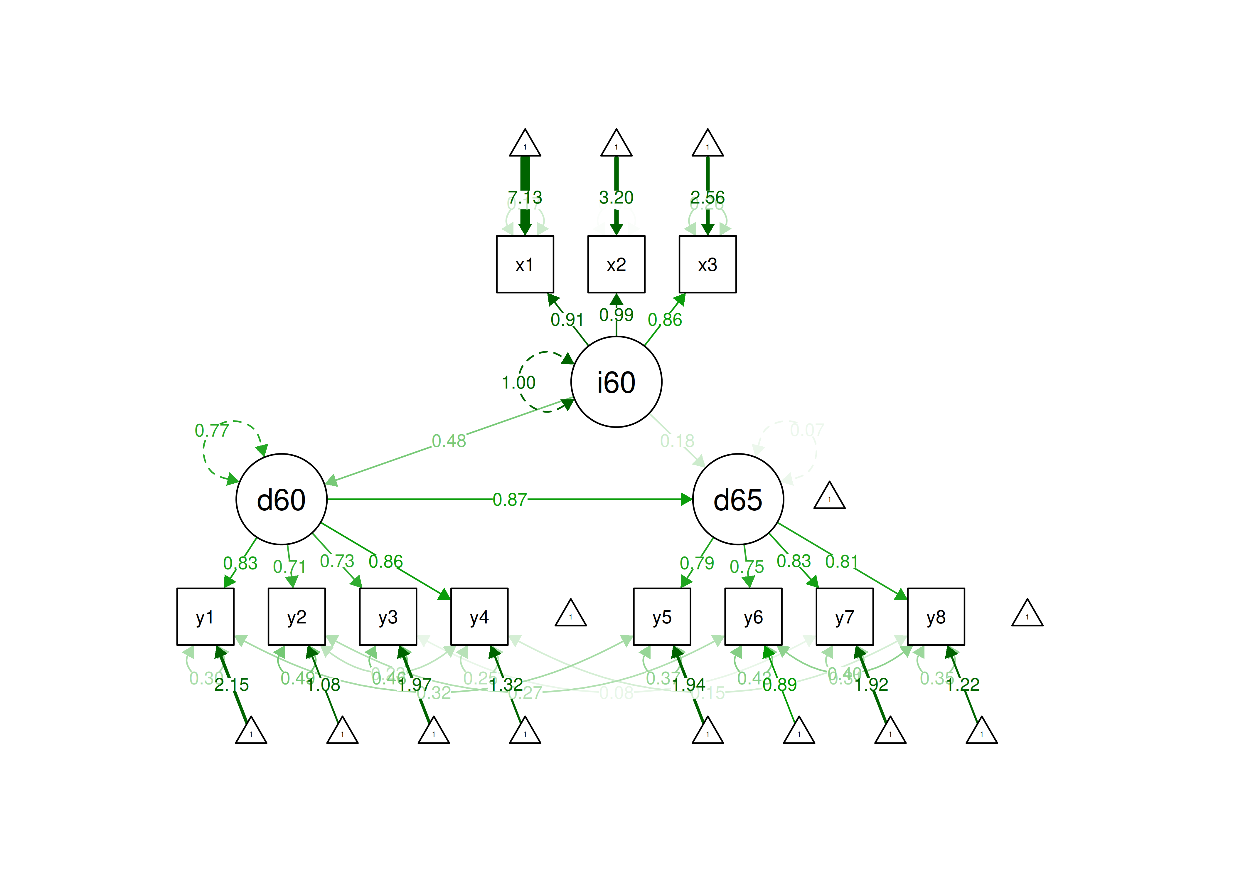
Figure 7.11: Example Structural Equation Model.
7.12 Benefits of SEM
There are many benefits of fitting a model in SEM (or in other latent variable approaches). First, unlike classical test theory, SEM can allow correlated errors. With SEM, you do not need to make as restrictive assumptions as in classical test theory. Second, unlike multiple regression, SEM can handle multiple dependent variables simultaneously. Third, SEM uses all available information (data) using a technique called full information maximum likelihood (FIML), even if participants have missing scores on some variables. By contrast, multiple regression and many other statistical analyses use listwise deletion, in which they discard participants if they have a missing score on any of the model variables. Fourth, whereas multiple regression assumes nonnormally distributed residuals, SEM can handle nonnormally distributed residuals via robust standard errors (i.e., MLR estimator) and robust fit indices. Fifth, SEM can estimate mediation in a single model.
Sixth, as described in the next section (7.12.1), SEM can be used to account for different forms of measurement error (e.g., method bias). Accounting for measurement error allows disattenuating associations with other constructs. I provide an example showing that SEM disattenuates associations for measurement error in Section 5.6.3. All of these benefits allow SEM to generate purer estimation of constructs, more accurate estimates of people’s levels on constructs, and more accurate estimates of associations between constructs. Our theories deal with constructs (latent variables), not with fallible measurements of constructs (manifest variables). Thus, SEM allows for models that are better aligned with theory than other statistical approaches that do not account for measurement error.
7.12.1 Accounting for Method Bias
SEM/CFA can be used to account for method biases and other forms of measurement error. You can use indicators that reflect different method biases, so that the method biases are discarded as unique errors, and are not combined in the “common variance” of the latent construct. SEM/CFA can be used to fit a multitrait-multimethod matrix to account for method variance. I provide an example of fitting a multitrait-multimethod matrix in CFA in Sections 5.3.1.4.2.5 and 14.4.2.13. But estimation of a multitrait-multimethod matrix in CFA can be challenging without making additional constraints/assumptions.
A more practical utility of SEM is that it allows one to obtain “purer” estimates of latent constructs (and people’s standing on them) by discarding measurement error, and you do not have to assume all errors are uncorrelated!
7.13 Guidelines for Reporting Reliability and Validity in SEM
Guidelines for reporting reliability and validity in structural equation modeling are provided by Cheung et al. (2024).
7.14 Power Analysis Using Monte Carlo Simulation
Power analysis for latent variable modeling approaches like SEM is more complicated than it is for other statistical analyses, such as correlation, multiple regression, t tests, analysis of variance, etc. Statistical power for these more straightforward analytical approaches can be estimated in G*Power (Faul et al., 2009): https://www.psychologie.hhu.de/arbeitsgruppen/allgemeine-psychologie-und-arbeitspsychologie/gpower.html (archived at https://perma.cc/F3RW-AXMQ)
I provide an example of how to conduct power analysis of an SEM model to determine the sample size needed to detect a hypothesized effect of a given effect size. To perform the power analysis, I use Monte Carlo simulation (Hancock & French, 2013; Muthén & Muthén, 2002). It is named after the Casino de Monte-Carlo in Monaco because Monte Carlo simulations involve random samples (random chance), as might be found in casino gambling. Monte Carlo simulations can be used to determine the sample size needed to detect a target parameter of a given effect size, using the following four steps (Y. A. Wang & Rhemtulla, 2021):
- Specify the sample size, a hypothesized true population SEM model, and all of its parameter values (e.g., factor loadings, intercepts, residuals, means, variances, covariances, regression paths, sample size);
- Generate a large number (e.g., 1,000) of random samples based on the hypothesized model and population values specified;
- Fit a SEM model to each of the generated samples, and for each one, record whether the target parameter is significantly different from zero;
- Calculate power as the proportion of simulated samples that produce a statistically significant estimate of the target parameter.
These four steps can be repeated with different sample sizes to identify the sample size that is needed to have a particular level of power (e.g., .80).
Power analysis of structural equation models using Monte Carlo simulation was estimated using the simsem package (Pornprasertmanit et al., 2021).
These examples were adapted from the simsem documentation:
https://github.com/simsem/simsem/wiki/Vignette (archived at https://perma.cc/BQF7-PQNK)
https://github.com/simsem/simsem/wiki/Example-18:-Simulation-with-Varying-Sample-Size (archived at https://perma.cc/8YCN-HENK)
https://github.com/simsem/simsem/wiki/Example-19:-Simulation-with-Varying-Sample-Size-and-Percent-Missing (archived at https://perma.cc/ZWL4-FHJ3)
https://github.com/simsem/simsem/blob/master/SupportingDocs/Examples/Version05/ex18/ex18.R (archived at https://perma.cc/5W93-BLFD)
https://github.com/simsem/simsem/blob/master/SupportingDocs/Examples/Version05/ex19/ex19.R (archived at https://perma.cc/7DJY-QYSW)
7.14.1 Specify Population Model
The population model was used to generate the simulated data. It is important to specify each parameter value in the population model based on theory and/or prior empirical research, especially meta-analysis of the target population (when possible).
Code
populationModel <- '
 #Specify measurement model factor loadings
 ind60 =~ .7*x1 + .7*x2 + .7*x3
 dem60 =~ .7*y1 + .7*y2 + .7*y3 + .7*y4
 dem65 =~ .7*y5 + .7*y6 + .7*y7 + .7*y8

 #Specify regression coefficients
 dem60 ~ .4*ind60
 dem65 ~ .25*ind60 + .85*dem60

 #Fix latent means to zero
 ind60 ~ 0
 dem60 ~ 0
 dem65 ~ 0

 #Fix latent variances to one
 ind60 ~~ 1*ind60
 dem60 ~~ 1*dem60
 dem65 ~~ 1*dem65

 #Specify covariances among latent variables (not necessary because the latent variables are already linked via regression paths)

 #Specify residual variances of manifest variables
 x1 ~~ (1-.7^2)*x1
 x2 ~~ (1-.7^2)*x2
 x3 ~~ (1-.7^2)*x3
 y1 ~~ (1-.7^2)*y1
 y2 ~~ (1-.7^2)*y2
 y3 ~~ (1-.7^2)*y3
 y4 ~~ (1-.7^2)*y4
 y5 ~~ (1-.7^2)*y5
 y6 ~~ (1-.7^2)*y6
 y7 ~~ (1-.7^2)*y7
 y8 ~~ (1-.7^2)*y8

 #Specify intercepts of manifest variables
 x1 ~ 0*1
 x2 ~ 0*1
 x3 ~ 0*1
 y1 ~ 0*1
 y2 ~ 0*1
 y3 ~ 0*1
 y4 ~ 0*1
 y5 ~ 0*1
 y6 ~ 0*1
 y7 ~ 0*1
 y8 ~ 0*1
'
7.14.1.1 Show the Model’s Fixed and Default Values
lavaan 0.6-20 did not run (perhaps do.fit = FALSE)?
** WARNING ** Estimates below are simply the starting values

  Estimator                                         ML
  Optimization method                           NLMINB
  Number of model parameters                         0

  Number of observations                             0


Parameter Estimates:


Latent Variables:
                   Estimate   Std.lv  Std.all
  ind60 =~
    x1                0.700    0.700    0.700
    x2                0.700    0.700    0.700
    x3                0.700    0.700    0.700
  dem60 =~
    y1                0.700    0.754    0.726
    y2                0.700    0.754    0.726
    y3                0.700    0.754    0.726
    y4                0.700    0.754    0.726
  dem65 =~
    y5                0.700    1.007    0.816
    y6                0.700    1.007    0.816
    y7                0.700    1.007    0.816
    y8                0.700    1.007    0.816

Regressions:
                   Estimate   Std.lv  Std.all
  dem60 ~
    ind60             0.400    0.371    0.371
  dem65 ~
    ind60             0.250    0.174    0.174
    dem60             0.850    0.636    0.636

Intercepts:
                   Estimate   Std.lv  Std.all
    ind60             0.000    0.000    0.000
   .dem60             0.000    0.000    0.000
   .dem65             0.000    0.000    0.000
   .x1                0.000    0.000    0.000
   .x2                0.000    0.000    0.000
   .x3                0.000    0.000    0.000
   .y1                0.000    0.000    0.000
   .y2                0.000    0.000    0.000
   .y3                0.000    0.000    0.000
   .y4                0.000    0.000    0.000
   .y5                0.000    0.000    0.000
   .y6                0.000    0.000    0.000
   .y7                0.000    0.000    0.000
   .y8                0.000    0.000    0.000

Variances:
                   Estimate   Std.lv  Std.all
    ind60             1.000    1.000    1.000
   .dem60             1.000    0.862    0.862
   .dem65             1.000    0.483    0.483
   .x1                0.510    0.510    0.510
   .x2                0.510    0.510    0.510
   .x3                0.510    0.510    0.510
   .y1                0.510    0.510    0.473
   .y2                0.510    0.510    0.473
   .y3                0.510    0.510    0.473
   .y4                0.510    0.510    0.473
   .y5                0.510    0.510    0.335
   .y6                0.510    0.510    0.335
   .y7                0.510    0.510    0.335
   .y8                0.510    0.510    0.335

R-Square:
                   Estimate
    dem60             0.138
    dem65             0.517
    x1                0.490
    x2                0.490
    x3                0.490
    y1                0.527
    y2                0.527
    y3                0.527
    y4                0.527
    y5                0.665
    y6                0.665
    y7                0.665
    y8                0.665
7.14.1.2 Model-Implied Covariance and Correlation Matrix
7.14.1.2.1 Model-implied covariance matrix:
$cov
      x1    x2    x3    y1    y2    y3    y4    y5    y6    y7    y8
x1 1.000
x2 0.490 1.000
x3 0.490 0.490 1.000
y1 0.196 0.196 0.196 1.078
y2 0.196 0.196 0.196 0.568 1.078
y3 0.196 0.196 0.196 0.568 0.568 1.078
y4 0.196 0.196 0.196 0.568 0.568 0.568 1.078
y5 0.289 0.289 0.289 0.532 0.532 0.532 0.532 1.525
y6 0.289 0.289 0.289 0.532 0.532 0.532 0.532 1.015 1.525
y7 0.289 0.289 0.289 0.532 0.532 0.532 0.532 1.015 1.015 1.525
y8 0.289 0.289 0.289 0.532 0.532 0.532 0.532 1.015 1.015 1.015 1.525

$mean
x1 x2 x3 y1 y2 y3 y4 y5 y6 y7 y8
 0  0  0  0  0  0  0  0  0  0  0
7.14.1.2.2 Model-implied correlation matrix
      x1    x2    x3    y1    y2    y3    y4    y5    y6    y7    y8
x1 1.000
x2 0.490 1.000
x3 0.490 0.490 1.000
y1 0.189 0.189 0.189 1.000
y2 0.189 0.189 0.189 0.527 1.000
y3 0.189 0.189 0.189 0.527 0.527 1.000
y4 0.189 0.189 0.189 0.527 0.527 0.527 1.000
y5 0.234 0.234 0.234 0.415 0.415 0.415 0.415 1.000
y6 0.234 0.234 0.234 0.415 0.415 0.415 0.415 0.665 1.000
y7 0.234 0.234 0.234 0.415 0.415 0.415 0.415 0.665 0.665 1.000
y8 0.234 0.234 0.234 0.415 0.415 0.415 0.415 0.665 0.665 0.665 1.000
7.14.2 Specify Analysis Model
Code
analysisModel_syntax <- '
 #Measurement model factor loadings (free the factor loading of the first indicator)
 ind60 =~ NA*x1 + x2 + x3
 dem60 =~ NA*y1 + y2 + y3 + y4
 dem65 =~ NA*y5 + y6 + y7 + y8

 #Regression paths
 dem60 ~ ind60
 dem65 ~ ind60 + dem60

 #Fix latent means to zero
 ind60 ~ 0
 dem60 ~ 0
 dem65 ~ 0

 #Fix latent variances to one
 ind60 ~~ 1*ind60
 dem60 ~~ 1*dem60
 dem65 ~~ 1*dem65

 #Estimate covariances among latent variables (not necessary because the latent variables are already linked via regression paths)

 #Estimate residual variances of manifest variables
 x1 ~~ x1
 x2 ~~ x2
 x3 ~~ x3
 y1 ~~ y1
 y2 ~~ y2
 y3 ~~ y3
 y4 ~~ y4
 y5 ~~ y5
 y6 ~~ y6
 y7 ~~ y7
 y8 ~~ y8

 #Free intercepts of manifest variables
 x1 ~ intx1*1
 x2 ~ intx2*1
 x3 ~ intx3*1
 y1 ~ inty1*1
 y2 ~ inty2*1
 y3 ~ inty3*1
 y4 ~ inty4*1
 y5 ~ inty5*1
 y6 ~ inty6*1
 y7 ~ inty7*1
 y8 ~ inty8*1
'
7.14.3 Specify Distribution of Data
Specifying the expected distributions of the data variables is an optional step, but it can help give you more realistic estimates of your likely power, especially when the data are non-normally distributed. First, identify the order in which the indicator variables appear in the model, so you can know the order to specify skewness and kurtosis (which I specify in the next section):
[1] "x1" "x2" "x3" "y1" "y2" "y3" "y4" "y5" "y6" "y7" "y8"Specify the skewness and kurtosis of the data variables. In this example, I set the variables \(x1\)–\(x3\) (the first three variables) to have skewness of 1.3 and kurtosis of 1.8, and I set the variables \(y1\)–\(y8\) (the next eight variables) to have a skewness of 2 and a kurtosis of 4.
7.14.4 Specify Extent and Type of Missing Data
7.14.4.1 Specify Missingness
Specifying the extent and pattern of missingness is an optional step, but it can help give you more realistic estimates of your likely power, especially when there is extensive missing data and/or the data are not missing completely at random (MCAR). For an example of specifying the extent and pattern of missingness in the context of a Monte Carlo power analysis, see Beaujean (2014). In this example, I set 10% of values to be missing for variables \(x1\), \(x2\), and \(x3\). I set 15% of values to be missing for variables \(y1\)–\(y8\). I assumed the missingness mechanism to be MCAR. To set missingness to be missing at random (MAR), add a covariate in the missingness formula (see Beaujean, 2014). I set the model to use full information maximum likelihood (FIML) estimation to handle missingness. If you set \(m\) to a value greater than zero, it will allow use of multiple imputation instead of FIML. Statistical power with multiple imputation tends to be lower than with FIML unless the number of imputations is large (J. Graham et al., 2007).
Code
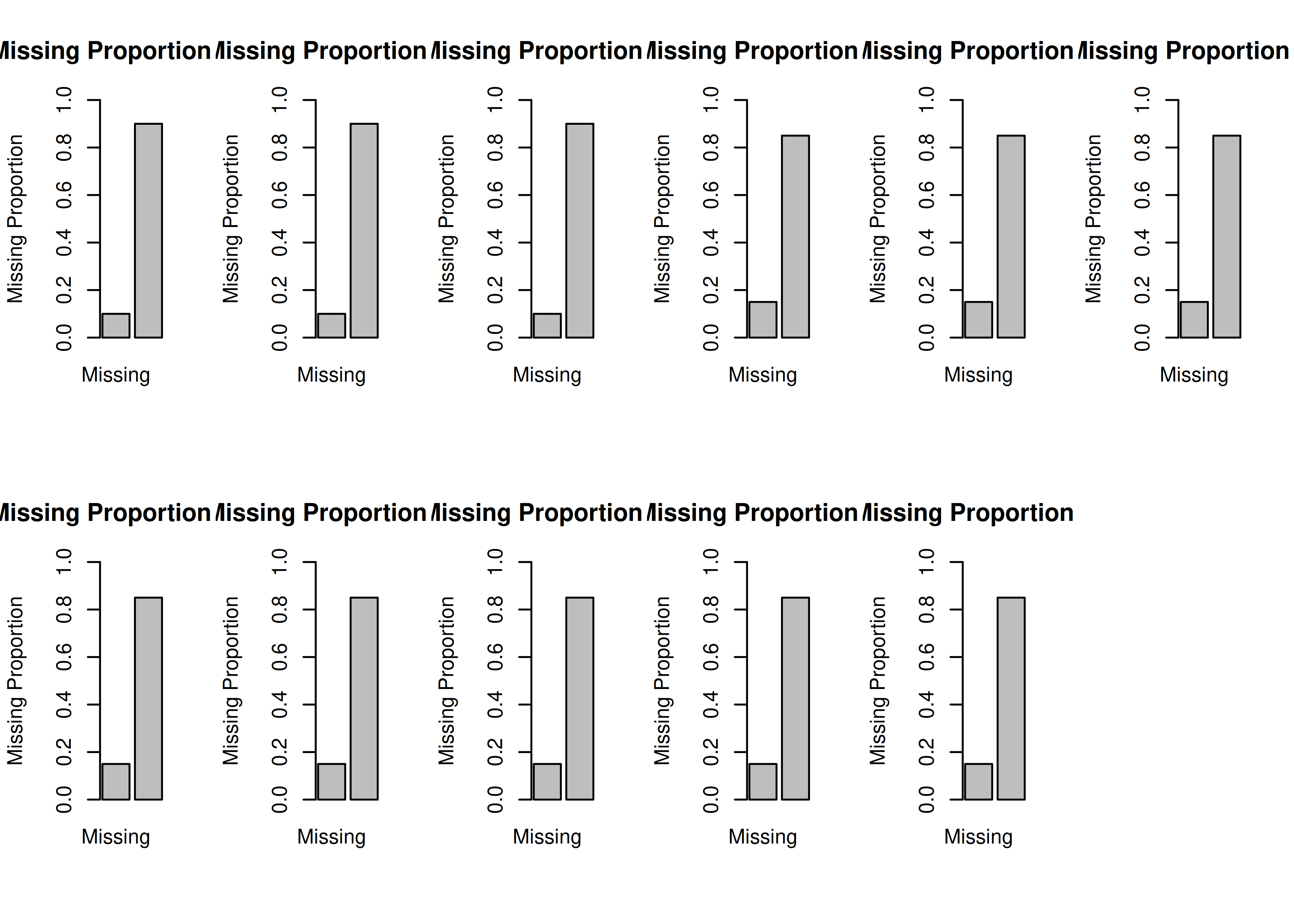
7.14.5 Specify Sample Sizes and Repetitions
Specify the sample sizes to evaluate in the Monte Carlo simulation and the number of repetitions per sample size.
7.14.6 Monte Carlo Simulation to Generate Data from the Population Parameter Values
Conduct Monte Carlo simulation with \(2\) repetitions per sample size \((N\text{s} = 150–700)\).
The multicore backend was used for parallel processing.
Parallel processing distributes a larger computation task across multiple computing processes or cores, and runs them simultaneously (in parallel) to speed up execution time (if multiple processes or cores are available).
If you choose to do processing in serial rather than parallel (by setting multicore = FALSE), you will need to run a special set.seed() command, prior to running the sim() command, to get reproducible results with those obtained from parallel processing: set.seed(seedNumber, "L'Ecuyer-CMRG"), where seedNumber is the value used for the seed.
Warning: this code takes a while to run based on \(551\) different sample sizes \((700 - 150 + 1)\) and \(2\) repetitions per sample size, for a total of \(1102\) iterations \(([700 - 150 + 1]\) sample sizes \(\times\) \(2\) repetitions per sample size \(= 1102\) iterations).
You can reduce the number of sample sizes and/or repetitions per sample size to be faster.
Code
Progress tracker is not available when 'multicore' is TRUE.Return the seed to the normal seed behavior so that future calls to set.seed() use the default settings:
7.14.7 Summary of Population Model
                 ind60=~x1 ind60=~x2 ind60=~x3 dem60=~y1 dem60=~y2 dem60=~y3
Population Value 0.7       0.7       0.7       0.7       0.7       0.7
                 dem60=~y4 dem65=~y5 dem65=~y6 dem65=~y7 dem65=~y8 dem60~ind60
Population Value 0.7       0.7       0.7       0.7       0.7       0.4
                 dem65~ind60 dem65~dem60 ind60~1 dem60~1 dem65~1 ind60~~ind60
Population Value 0.25        0.85        0       0       0       1
                 dem60~~dem60 dem65~~dem65 x1~~x1 x2~~x2 x3~~x3 y1~~y1 y2~~y2
Population Value 1            1            0.51   0.51   0.51   0.51   0.51
                 y3~~y3 y4~~y4 y5~~y5 y6~~y6 y7~~y7 y8~~y8 x1~1 x2~1 x3~1 y1~1
Population Value 0.51   0.51   0.51   0.51   0.51   0.51   0    0    0    0
                 y2~1 y3~1 y4~1 y5~1 y6~1 y7~1 y8~1
Population Value 0    0    0    0    0    0    0
7.14.8 Summary of Simulated Data
RESULT OBJECT
Model Type
[1] "lavaan"
========= Fit Indices Cutoffs ============
    N chisq.scaled       aic       bic rmsea.scaled cfi.scaled tli.scaled  srmr
1 150       70.294  4048.832  4165.404        0.060          1      1.027 0.057
2 288       67.290  7631.650  7760.196        0.050          1      1.022 0.049
3 425       64.307 11188.506 11328.938        0.041          1      1.017 0.042
4 562       61.324 14745.362 14897.681        0.031          1      1.012 0.034
5 700       58.319 18328.181 18492.473        0.021          1      1.007 0.027
========= Parameter Estimates and Standard Errors ============
            Estimate Average Estimate SD Average SE Power (Not equal 0) Std Est
ind60=~x1              0.698       0.075      0.070               1.000   0.700
ind60=~x2              0.698       0.075      0.070               1.000   0.700
ind60=~x3              0.697       0.073      0.070               1.000   0.698
dem60=~y1              0.698       0.081      0.078               1.000   0.708
dem60=~y2              0.698       0.077      0.077               1.000   0.710
dem60=~y3              0.696       0.078      0.077               1.000   0.707
dem60=~y4              0.692       0.081      0.077               1.000   0.701
dem65=~y5              0.690       0.079      0.071               1.000   0.793
dem65=~y6              0.690       0.080      0.071               1.000   0.795
dem65=~y7              0.689       0.079      0.072               1.000   0.794
dem65=~y8              0.690       0.081      0.072               1.000   0.794
dem60~ind60            0.403       0.096      0.092               0.989   0.370
dem65~ind60            0.260       0.108      0.105               0.713   0.178
dem65~dem60            0.866       0.162      0.141               1.000   0.634
x1~~x1                 0.502       0.081      0.076               0.997   0.507
x2~~x2                 0.502       0.084      0.076               0.998   0.507
x3~~x3                 0.505       0.080      0.077               0.998   0.509
y1~~y1                 0.561       0.090      0.086               0.999   0.496
y2~~y2                 0.557       0.094      0.085               1.000   0.494
y3~~y3                 0.563       0.092      0.086               1.000   0.498
y4~~y4                 0.572       0.092      0.087               0.999   0.505
y5~~y5                 0.589       0.100      0.093               1.000   0.369
y6~~y6                 0.583       0.101      0.091               1.000   0.367
y7~~y7                 0.584       0.099      0.091               1.000   0.368
y8~~y8                 0.586       0.105      0.092               1.000   0.368
intx1                  0.000       0.057      0.053               0.050  -0.002
intx2                  0.000       0.056      0.053               0.053  -0.002
intx3                  0.001       0.055      0.053               0.049  -0.001
inty1                  0.002       0.058      0.058               0.043  -0.001
inty2                  0.000       0.059      0.058               0.052  -0.002
inty3                  0.003       0.057      0.058               0.045   0.000
inty4                  0.004       0.060      0.058               0.056   0.001
inty5                  0.001       0.070      0.068               0.057  -0.002
inty6                  0.000       0.070      0.068               0.052  -0.003
inty7                  0.001       0.071      0.068               0.049  -0.002
inty8                  0.000       0.071      0.068               0.062  -0.003
            Std Est SD Std Ave SE r_coef.n r_se.n
ind60=~x1        0.055      0.051    0.053 -0.804
ind60=~x2        0.055      0.051   -0.011 -0.795
ind60=~x3        0.053      0.052    0.050 -0.789
dem60=~y1        0.051      0.048    0.032 -0.747
dem60=~y2        0.050      0.048   -0.012 -0.754
dem60=~y3        0.051      0.048   -0.013 -0.766
dem60=~y4        0.052      0.048    0.012 -0.742
dem65=~y5        0.038      0.035    0.106 -0.740
dem65=~y6        0.039      0.035    0.106 -0.739
dem65=~y7        0.037      0.035    0.107 -0.735
dem65=~y8        0.037      0.035    0.126 -0.757
dem60~ind60      0.075      0.072   -0.036 -0.796
dem65~ind60      0.071      0.070   -0.019 -0.800
dem65~dem60      0.070      0.063   -0.087 -0.678
x1~~x1           0.077      0.072    0.035 -0.733
x2~~x2           0.078      0.071    0.073 -0.737
x3~~x3           0.074      0.072    0.050 -0.726
y1~~y1           0.072      0.068    0.028 -0.531
y2~~y2           0.070      0.067    0.069 -0.558
y3~~y3           0.071      0.068    0.049 -0.634
y4~~y4           0.072      0.067   -0.050 -0.585
y5~~y5           0.060      0.056    0.054 -0.559
y6~~y6           0.062      0.055    0.025 -0.562
y7~~y7           0.058      0.056    0.002 -0.625
y8~~y8           0.058      0.056    0.019 -0.521
intx1            0.058      0.054    0.037 -0.919
intx2            0.056      0.054    0.028 -0.917
intx3            0.055      0.054    0.061 -0.921
inty1            0.056      0.055    0.002 -0.902
inty2            0.057      0.055   -0.020 -0.907
inty3            0.055      0.055   -0.014 -0.916
inty4            0.058      0.055   -0.056 -0.909
inty5            0.057      0.054    0.022 -0.904
inty6            0.056      0.054    0.003 -0.906
inty7            0.057      0.054    0.007 -0.909
inty8            0.057      0.054    0.027 -0.903
========= Correlation between Fit Indices ============
             chisq.scaled    aic    bic rmsea.scaled cfi.scaled tli.scaled
chisq.scaled        1.000 -0.175 -0.175        0.918     -0.826     -0.903
aic                -0.175  1.000  1.000       -0.386      0.422      0.305
bic                -0.175  1.000  1.000       -0.386      0.422      0.305
rmsea.scaled        0.918 -0.386 -0.386        1.000     -0.922     -0.933
cfi.scaled         -0.826  0.422  0.422       -0.922      1.000      0.944
tli.scaled         -0.903  0.305  0.305       -0.933      0.944      1.000
srmr                0.547 -0.805 -0.806        0.700     -0.717     -0.656
n                  -0.175  0.999  0.999       -0.386      0.422      0.305
               srmr      n
chisq.scaled  0.547 -0.175
aic          -0.805  0.999
bic          -0.806  0.999
rmsea.scaled  0.700 -0.386
cfi.scaled   -0.717  0.422
tli.scaled   -0.656  0.305
srmr          1.000 -0.805
n            -0.805  1.000
================== Replications =====================
Number of replications = 1102
Number of converged replications = 1102
Number of nonconverged replications:
   1. Nonconvergent Results = 0
   2. Nonconvergent results from multiple imputation = 0
   3. At least one SE were negative or NA = 0
   4. Nonpositive-definite latent or observed (residual) covariance matrix
      (e.g., Heywood case or linear dependency) = 0
NOTE: The sample size is varying.
NOTE: The data generation model is not the same as the analysis model. See the summary of the population underlying data generation by the summaryPopulation function.7.14.10 Time to Completion
============ Wall Time ============
  1. Error Checking and setting up data-generation and analysis template:        0.001
  2. Set combinations of n, pmMCAR, and pmMAR:                                   0.001
  3. Setting up simulation conditions for each replication:                      0.019
  4. Total time elapsed running all replications:                             1279.727
  5. Combining outputs from different replications:                              0.075

============ Average Time in Each Replication ============
  1. Data Generation:                                  0.082
  2. Impose Missing Values:                            0.014
  3. User-defined Data-Transformation Function:        0.000
  4. Main Data Analysis:                               2.705
  5. Extracting Outputs:                               1.810

============ Summary ============
  Start Time:                   2025-12-04 12:15:05
  End Time:                     2025-12-04 12:36:25
  Wall (Actual) Time:             1279.823
  System (Processors) Time:       5081.384
  Units:                        seconds
7.14.11 Cutoffs of Fit Indices

7.14.12 Statistical Power
7.14.12.1 Plot of Power to Detect Various Parameters as a Function of Sample Size
At \(\alpha = .05\); dashed horizontal line represents power (\(1 - \beta\)) of .8
Code
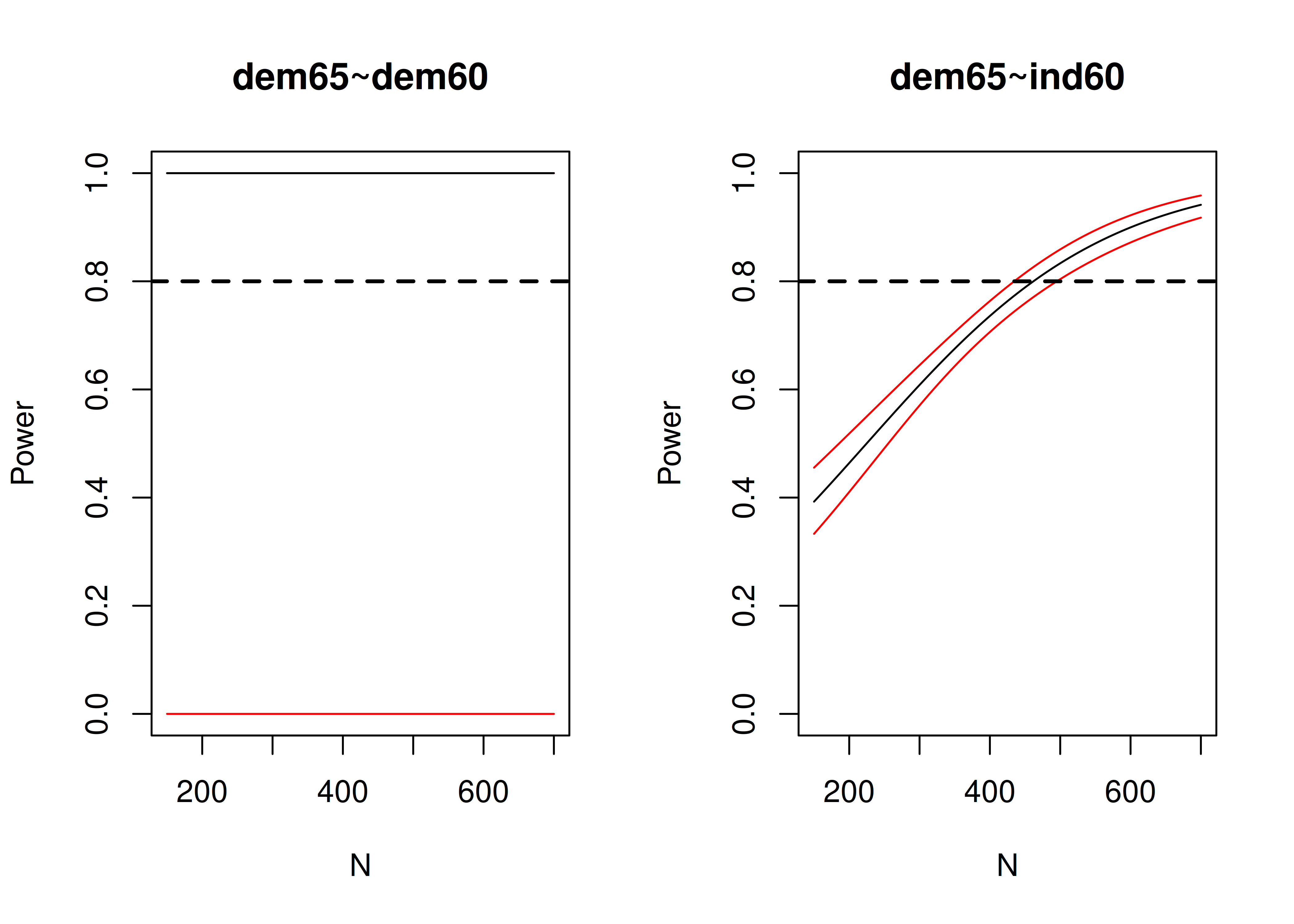
Figure 7.14: Plot of Power to Detect Various Parameters as a Function of Sample Size, From Monte Carlo Power Analysis.
7.14.12.2 Sample Size Needed to Detect a Given Parameter
At power (\(1 - \beta\)) = .80, \(\alpha = .05\)
Code
  ind60=~x1   ind60=~x2   ind60=~x3   dem60=~y1   dem60=~y2   dem60=~y3
        Inf         Inf         Inf         Inf         Inf         Inf
  dem60=~y4   dem65=~y5   dem65=~y6   dem65=~y7   dem65=~y8 dem60~ind60
        Inf         Inf         Inf         Inf         Inf         150
dem65~ind60 dem65~dem60      x1~~x1      x2~~x2      x3~~x3      y1~~y1
        476         Inf         150         150         150         150
     y2~~y2      y3~~y3      y4~~y4      y5~~y5      y6~~y6      y7~~y7
        Inf         Inf         150         Inf         Inf         Inf
     y8~~y8       intx1       intx2       intx3       inty1       inty2
        Inf          NA          NA          NA          NA          NA
      inty3       inty4       inty5       inty6       inty7       inty8
         NA          NA          NA          NA          NA          NA
7.14.12.3 Power to Detect Each Parameter at a Given Sample Size
At \(N = 200\), \(\alpha = .05\)
     iv.N ind60=~x1 ind60=~x2 ind60=~x3 dem60=~y1 dem60=~y2 dem60=~y3 dem60=~y4
[1,]  200         1         1         1         1         1         1         1
     dem65=~y5 dem65=~y6 dem65=~y7 dem65=~y8 dem60~ind60 dem65~ind60
[1,]         1         1         1         1   0.9556141   0.4424786
     dem65~dem60   x1~~x1    x2~~x2    x3~~x3    y1~~y1 y2~~y2 y3~~y3    y4~~y4
[1,]           1 0.989442 0.9955458 0.9928039 0.9968834      1      1 0.9999989
     y5~~y5 y6~~y6 y7~~y7 y8~~y8      intx1      intx2      intx3      inty1
[1,]      1      1      1      1 0.07074849 0.06634111 0.04408819 0.04152705
          inty2      inty3      inty4      inty5      inty6      inty7
[1,] 0.05062411 0.03905802 0.07232276 0.06501033 0.05624485 0.04991777
          inty8
[1,] 0.05576067
7.15 Generalizability Theory
There are also SEM approaches for performing generalizability theory analyses. The reader is referred to examples by Vispoel et al. (2018), Vispoel et al. (2019), Vispoel et al. (2022), and Vispoel et al. (2023).
7.16 Conclusion
Structural equation modeling (SEM) is an advanced modeling approach that allows estimating latent variables as the common variance from multiple measures. SEM holds promise to account for measurement error and method biases, which allows one to get more accurate estimates of constructs, people’s standing on constructs (i.e., individual differences), and associations between constructs.
7.17 Suggested Readings
MacCallum & Austin (2000)
7.18 Exercises
7.18.1 Questions
Note: Several of the following questions use data from the Children of the National Longitudinal Survey of Youth Survey (CNLSY). The CNLSY is a publicly available longitudinal data set provided by the Bureau of Labor Statistics (https://www.bls.gov/nls/nlsy79-children.htm#topical-guide; archived at https://perma.cc/EH38-HDRN). The CNLSY data file for these exercises is located on the book’s page of the Open Science Framework (https://osf.io/3pwza). Children’s behavior problems were rated in 1988 (time 1: T1) and then again in 1990 (time 2: T2) on the Behavior Problems Index (BPI). Below are the items corresponding to the Antisocial subscale of the BPI:
- cheats or tells lies
- bullies or is cruel/mean to others
- does not seem to feel sorry after misbehaving
- breaks things deliberately
- is disobedient at school
- has trouble getting along with teachers
- has sudden changes in mood or feeling
Fit a confirmatory factor analysis model to the seven items of the Antisocial subscale of the Behavior Problems Index at T1. Set the first indicator to be the referent indicator (to set the scale of the latent factor) by setting its loading to one. Allow the factor loadings of the other indicators to be freely estimated. Set the mean (intercept) of the latent factor to be zero. Do not allow the residuals to be correlated. Use full information maximum likelihood (FIML) to account for missing data. Use robust standard errors to account for non-normally distributed data.
- This is an over-simplification, but for now let us assume a model fits “well” if CFI \(\geq .95\), RMSEA \(< .08\), and SRMR \(< .08\) (Schreiber et al., 2006). Did the model fit well? What does this indicate?
- Examine the modification indices. Which modification would result in the greatest improvement in model fit? Why do you think this modification would improve model fit?
Fit the modified confirmatory factor analysis model to make the suggested revision you identified in
1b.- Provide a figure of the model with standardized coefficients.
- The modified model and the original model are considered “nested” models. The original model is nested within the modified model because the modified model includes all of the terms of the original model along with additional terms. Model fit of nested models can be directly compared with a chi-square difference test. Did the modified model fit better than the original model?
- Did the modified model fit well? What does this indicate? Which item is most strongly with the latent factor? Which item is most weakly associated with the latent factor?
- What is the estimate of internal consistency reliability of the items, based on coefficient omega?
Fit a confirmatory factor analysis model to the seven items of the Antisocial subscale of the Behavior Problems Index at both T1 and T2 simultaneously in the same model. Allow the items at T1 to load onto a different factor than the items at T2 (i.e., a two-factor model—one antisocial at each time point). Set the scale of the latent factors by standardizing the latent factors—set their means to one and their variances to zero. This allows you to freely estimate the factor loadings of all items (instead of setting a reference indicator). Estimate the covariance between the two latent factors. Treat exogenous covariates as random variables (whose means, variances, and covariances are estimated) by specifying
fixed.x = FALSE. Use full information maximum likelihood (FIML) to account for missing data. Use robust standard errors to account for non-normally distributed data. Apply the same modification you noted in 1b above to each factor.- Because the two latent factors are standardized, the “covariance” path between the two latent factors represents a correlation.
What is the correlation between the latent factors?
What is the correlation between the sum scores (
bpi_antisocialT1Sum,bpi_antisocialT2Sum)? Which is greater and why? - Change the covariance path to a regression path from the latent factor at T1 predicting the latent factor at T2.
Also include the sum score of anxious/depressed symptoms at T1 (
bpi_anxiousDepressedSum) as a predictor of antisocial behavior at T2. Do anxious/depressed symptoms at T1 predict antisocial behavior at T2 controlling for prior levels of antisocial behavior at T1? Interpret the findings.
- Because the two latent factors are standardized, the “covariance” path between the two latent factors represents a correlation.
What is the correlation between the latent factors?
What is the correlation between the sum scores (
You plan to conduct a study that would examine whether stress and harsh parenting predict children’s antisocial behavior. Your hypothesis is that stress and harsh parenting both lead to children’s antisocial behavior. You would like to apply for a grant to test these hypotheses, but you first want to know what sample size you would need to have adequate power to detect the hypothesized effects. Because you read this book, you remember that measurement error attenuates the associations you would observe, which would make it less likely that you would be able to detect the true effect (if there truly is an effect). As a result, you plan to assess each construct with multiple measurement methods/measures. You plan to model each construct with a latent variable in a structural equation modeling framework to account for measurement error and disattenuate the associations, which will make the associations more closely approximate the true effect and will make it more likely that you will detect the effect if it exists. You plan to assess stress with three methods (self-report, friend report, cortisol), harsh parenting with four methods (parents’ self-report, spousal report, child report, observation), and children’s antisocial behavior with four methods (parent report, teacher report, child report, observation).
You conduct a power analysis with the following assumptions that you made based on theory and prior empirical research:
- The factor loading for each measure on its latent variable is .75
- Stress influences children’s antisocial behavior with a regression coefficient of .20
- Harsh parenting influences children’s antisocial behavior with a regression coefficient of .45
- Stress influences harsh parenting with a regression coefficient of .4
Set the intercepts of the indicators to zero. Set the scale of the latent factors by standardizing the latent factors—set their means to one and their variances to zero. Do not estimate correlated errors. You expect each measure to show 10% missingness, and for missingness to be completely at random (MCAR). Use full information maximum likelihood (FIML) to handle missing values. As is common with measures in clinical psychology, you expect each measure to be positively skewed with a skewness of 2.5 and leptokurtic with a kurtosis of 5. Use robust standard errors to account for non-normally distributed data. Using a seed of 52242, an alpha level of .05, and one repetition per sample size, in the
simsempackage:- What sample size would you need to have adequate power to detect the effect of stress on antisocial behavior and the effect of harsh parenting on antisocial behavior?
- Due to financial and time constraints of the grant, you are only able to collect a sample size of 150. What power would you have to detect the effect of stress on antisocial behavior and the effect of harsh parenting on antisocial behavior?
- Your study finds that neither stress nor harsh parenting predicts antisocial behavior. How would you interpret each of these findings?
- Re-run the power analysis with normally distributed values (skewness \(= 0\), kurtosis \(= 0\)), using 50 repetitions with a sample size of 150. Did power to detect the hypothesized effects increase or decrease? What does this indicate?
7.18.2 Answers
- The model did not fit well according to CFI \((0.88)\) and RMSEA \((0.09)\). SRMR \((0.05)\) was acceptable. The poor model fit indicates that it is unlikely that the causal process described by the hypothesized model gave rise to the observed data.
- The modification that would result in the greatest model fit according to the modification indices is to allow indicators 5 and 6 to be correlated. These indicators reflect “disobedience at school” and “trouble getting along with teachers,” respectively. It is likely that allowing these two residuals to correlate would improve model fit because they both assess children’s behavior in the school context, and so they would continue to be associated with each other even after accounting for variance from the latent factor.
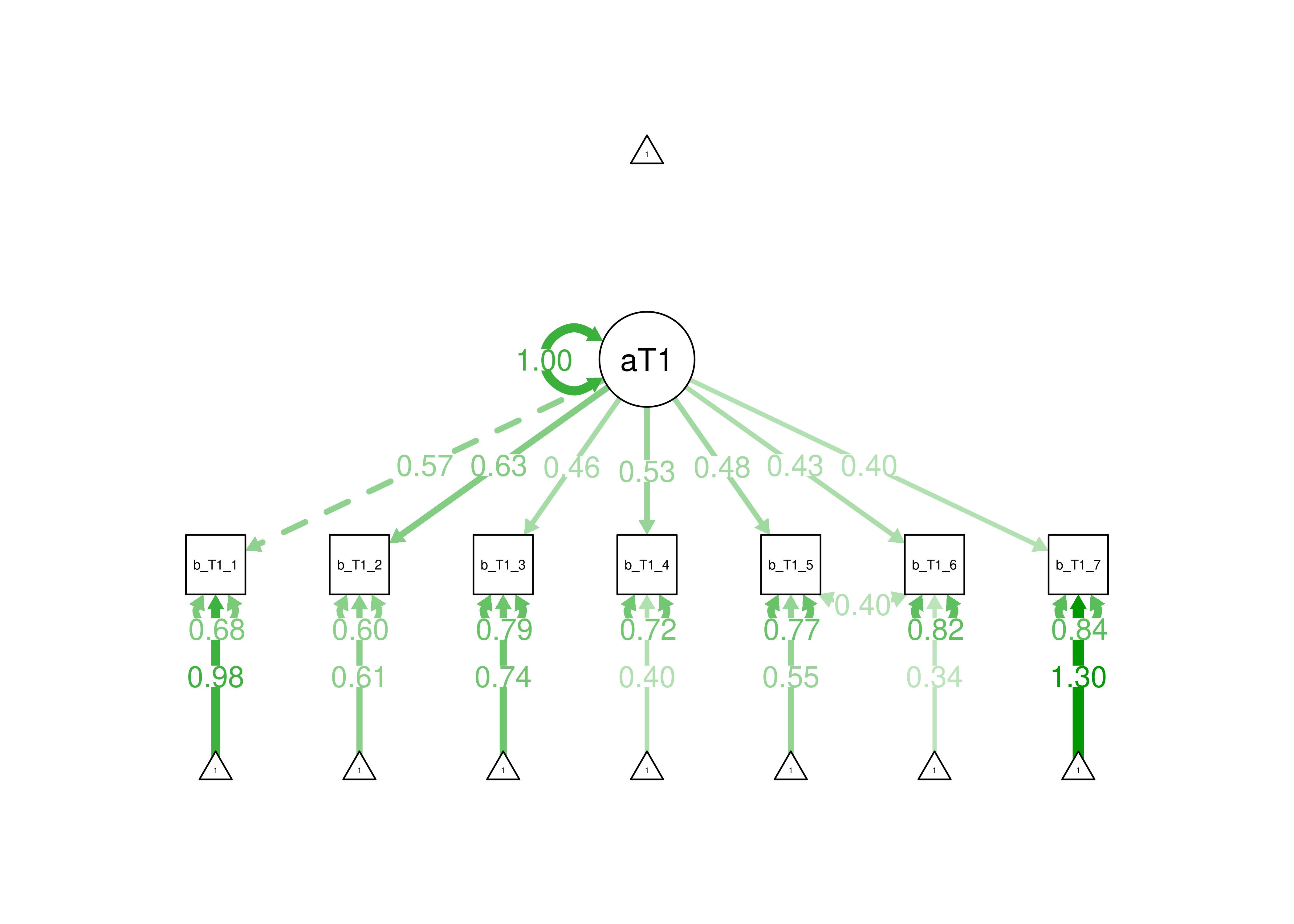
Figure 7.15: Figure of the Confirmatory Factor Analysis Model With Standardized Coefficients.
- The modified model \((\chi^2[df = 13] = 33.68)\) fit significantly better than the original model \((\chi^2[df = 14] = 391.38)\) according to a chi-square difference test \((\Delta\chi^2[df = 1] = 833.51, p < .001)\).
- The model fit well according to CFI \((0.9923114)\), RMSEA \((0.02416)\), and SRMR \((0.0133989)\). This indicates that there is evidence that one factor may do a good job of explaining the covariance among the indicators, especially when allowing the residuals of items 5 and 6 to correlate. The item that shows the strongest association with the latent factor is item 2 (“bullies or is cruel/mean to others”: standardized factor loading = \(.63\)). The item that shows the weakest association with the latent factor is item 7 (“sudden changes in mood or feeling”: standardized factor loading = \(.40\)). Thus, meanness seems more core to the construct of antisocial behavior compared to sudden mood changes.
- The estimate of internal consistency reliability of items, based on coefficient omega (\(\omega\)), is \(.68\).
- The correlation between the latent factor at T1 and T2 is \(\phi = .76\). The correlation between the sum score at T1 and T2 is \(r = .50\). This indicates that the correlation of individual differences across time (rank-order stability) is stronger for the latent factor than for the sum scores. This is likely because the latent factors account for measurement error whereas the sum scores do not, and associations are attenuated due to measurement error. Thus, the association of the latent factor at T1 and T2 likely more accurately reflects the “true” cross-time association of the construct (compared to the association of the sum scores at T1 and T2).
- Yes, anxious/depressed symptoms significantly predicted antisocial behavior at T2 while controlling for prior levels of antisocial behavior \((B = 0.11, β = .11, SE = 0.02, p < .001)\). That is, anxious/depressed symptoms predicted relative (rank-order) changes in antisocial behavior from T1 to T2. This suggests that anxiety/depression may be a pathway to antisocial behavior for some children. Because the data come from an observational design, however, we cannot infer causality. For instance, the association could owe to the opposite direction of effect (antisocial behavior could lead to anxiety/depression) or to a third variable (e.g., victimization could lead to both antisocial behavior and anxiety/depression; i.e., antisocial behavior and anxiety/depression could share a common cause).
- You would need a sample size of \(609\) to detect the effect of stress on children’s antisocial behavior. You would need a sample size of \(100\) to detect the effect of harsh parenting on children’s antisocial behavior.
- You would have a power of \(.22\) to detect the effect of stress on children’s antisocial behavior. You would have a power of \(.91\) to detect the effect of harsh parenting on children’s antisocial behavior.
- Because your study was well-powered to detect the effect of harsh parenting (\(\text{power} = .91\)) and you found no statistically significant association between harsh parenting and children’s antisocial behavior, it suggests that harsh parenting did not influence antisocial behavior in this sample (at least not with a large enough effect size to be practically significant). Because your study was under-powered to detect the effect of stress (\(\text{power} = .22\)) and you found no statistically significant association between stress and children’s antisocial behavior, we do not know whether you did not detect an association because (a) stress did not influence antisocial behavior in this sample (i.e., your hypotheses were incorrect), or (b) there was an effect of stress (i.e., your hypotheses were correct), but your sample size was too small and/or your measurements were too unreliable to detect the effect given the effect size.
- Power to detect the hypothesized effects increased when the data were normally distributed (compared to when the data were non-normally distributed). You would have a power of \(.40\) to detect the effect of stress on children’s antisocial behavior. You would have a power of \(1.00\) to detect the effect of harsh parenting on children’s antisocial behavior. This indicates that statistical power tends to be lower when data are non-normally distributed (compared to when data are normally distributed).