I want your feedback to make the book better for you and other readers. If you find typos, errors, or places where the text may be improved, please let me know. The best ways to provide feedback are by GitHub or hypothes.is annotations.
Opening an issue or submitting a pull request on GitHub: https://github.com/isaactpetersen/Principles-Psychological-Assessment
Adding an annotation using hypothes.is.
To add an annotation, select some text and then click the
symbol on the pop-up menu.
To see the annotations of others, click the
symbol in the upper right-hand corner of the page.
Chapter 14 Factor Analysis and Principal Component Analysis
“It can scarcely be denied that the supreme goal of all theory is to make the irreducible basic elements as simple and as few as possible without having to surrender the adequate representation of a single datum of experience.”
— Albert Einstein (1934, p. 165); sometimes paraphrased as “Everything should be made as simple as possible, but not simpler.”
14.1 Overview of Factor Analysis
Factor analysis is a class of latent variable models that is designated to identify the structure of a measure or set of measures, and ideally, a construct or set of constructs. It aims to identify the optimal latent structure for a group of variables. Factor analysis encompasses two general types: confirmatory factor analysis and exploratory factor analysis. Exploratory factor analysis (EFA) is a latent variable modeling approach that is used when the researcher has no a priori hypotheses about how a set of variables is structured. EFA seeks to identify the empirically optimal-fitting model in ways that balance accuracy (i.e., variance accounted for) and parsimony (i.e., simplicity). Confirmatory factor analysis (CFA) is a latent variable modeling approach that is used when a researcher wants to evaluate how well a hypothesized model fits, and the model can be examined in comparison to alternative models. Using a CFA approach, the researcher can pit models representing two theoretical frameworks against each other to see which better accounts for the observed data.
Factor analysis is considered to be a “pure” data-driven method for identifying the structure of the data, but the “truth” that we get depends heavily on the decisions we make regarding the parameters of our factor analysis (Floyd & Widaman, 1995; Sarstedt et al., 2024). The goal of factor analysis is to identify simple, parsimonious factors that underlie the “junk” (i.e., scores filled with measurement error) that we observe.
It used to take a long time to calculate a factor analysis because it was computed by hand. Now, it is fast to compute factor analysis with computers (e.g., oftentimes less than 30 ms). In the 1920s, Spearman developed factor analysis to understand the factor structure of intelligence. It was a long process—it took Spearman around one year to calculate the first factor analysis! Factor analysis takes a large dimension data set and simplifies it into a smaller set of factors that are thought to reflect underlying constructs. If you believe that nature is simple underneath, factor analysis gives nature a chance to display the simplicity that lives beneath the complexity on the surface. Spearman identified a single factor, g, that accounted for most of the covariation between the measures of intelligence.
Factor analysis involves observed (manifest) variables and unobserved (latent) factors. In a reflective model, it is assumed that the latent factor influences the manifest variables, and the latent factor therefore reflects the common (reliable) variance among the variables. A factor model potentially includes factor loadings, residuals (errors or disturbances), intercepts/means, covariances, and regression paths. A regression path indicates a hypothesis that one variable (or factor) influences another. The standardized regression coefficient represents the strength of association between the variables or factors. A factor loading is a regression path from a latent factor to an observed (manifest) variable. The standardized factor loading represents the strength of association between the variable and the latent factor. A residual is variance in a variable (or factor) that is unexplained by other variables or factors. An indicator’s intercept is the expected value of the variable when the factor(s) (onto which it loads) is equal to zero. Covariances are the associations between variables (or factors). A covariance path between two variables represents omitted shared cause(s) of the variables. For instance, if you depict a covariance path between two variables, it means that there is a shared cause of the two variables that is omitted from the model (for instance, if the common cause is not known or was not assessed).
In factor analysis, the relation between an indicator (\(\text{X}\)) and its underlying latent factor(s) (\(\text{F}\)) can be represented with a regression formula as in Equation (14.1):
\[\begin{equation} \text{X} = \lambda \cdot \text{F} + \text{Item Intercept} + \text{Error Term} \tag{14.1} \end{equation}\]
where:
- \(\text{X}\) is the observed value of the indicator
- \(\lambda\) is the factor loading, indicating the strength of the association between the indicator and the latent factor(s)
- \(\text{F}\) is the person’s value on the latent factor(s)
- \(\text{Item Intercept}\) represents the constant term that accounts for the expected value of the indicator when the latent factor(s) are zero
- \(\text{Error Term}\) is the residual, indicating the extent of variance in the indicator that is not explained by the latent factor(s)
When the latent factors are uncorrelated, the (standardized) error term for an indicator is calculated as 1 minus the sum of squared standardized factor loadings for a given item (including cross-loadings).
Another class of factor analysis models are higher-order (or hierarchical) factor models and bifactor models. Guidelines in using higher-order factor and bifactor models are discussed by Markon (2019).
Factor analysis is a powerful technique to help identify the factor structure that underlies a measure or construct. As discussed in Section 14.1.4, however, there are many decisions to make in factor analysis, in addition to questions about which variables to use, how to scale the variables, etc. (Floyd & Widaman, 1995; Sarstedt et al., 2024). If the variables going into a factor analysis are not well assessed, factor analysis will not rescue the factor structure. In such situations, there is likely to be the problem of garbage in, garbage out. Factor analysis depends on the covariation among variables. Given the extensive method variance that measures have, factor analysis (and principal component analysis) tends to extract method factors. Method factors are factors that are related to the methods being assessed rather than the construct of interest. However, multitrait-multimethod approaches to factor analysis (such as in Section 14.4.2.13) help better partition the variance in variables that reflects method variance versus construct variance, to get more accurate estimates of constructs.
Floyd & Widaman (1995) provide an overview of factor analysis for the development of clinical assessments.
14.1.1 Example Factor Models from Correlation Matrices
Before pursuing factor analysis, it is helpful to evaluate the extent to which the variables are intercorrelated. If the variables are not correlated (or are correlated only weakly), there is no reason to believe that a common factor influences them, and thus factor analysis would not be useful. So, before conducting a factor analysis, it is important to examine the correlation matrix of the variables to determine whether the variables intercorrelate strongly enough to justify a factor analysis.
Below, I provide some example factor models from various correlation matrices. Analytical examples of factor analysis are presented in Section 14.4.
Consider the example correlation matrix in Figure 14.1. Because all of the correlations are the same (\(r = .60\)), we expect there is approximately one factor for this pattern of data.
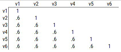
Figure 14.1: Example Correlation Matrix 1.
In a single-factor model fit to these data, the factor loadings are .77 and the residual error terms are .40, as depicted in Figure 14.2. The amount of common variance (\(R^2\)) that is accounted for by an indicator is estimated as the square of the standardized loading: \(.60 = .77 \times .77\). The amount of error for an indicator is estimated as: \(\text{error} = 1 - \text{common variance}\), so in this case, the amount of error is: \(.40 = 1 - .60\). The proportion of the total variance in indicators that is accounted for by the latent factor is the sum of the square of the standardized loadings divided by the number of indicators. That is, to calculate the proportion of the total variance in the variables that is accounted for by the latent factor, you would square the loadings, sum them up, and divide by the number of variables: \(\frac{.77^2 + .77^2 + .77^2 + .77^2 + .77^2 + .77^2}{6} = \frac{.60 + .60 + .60 + .60 + .60 + .60}{6} = .60\). Thus, the latent factor accounts for 60% of the variance in the indicators. In this model, the latent factor explains the covariance among the variables. If the answer is simple, a small and parsimonious model should be able to obtain the answer.
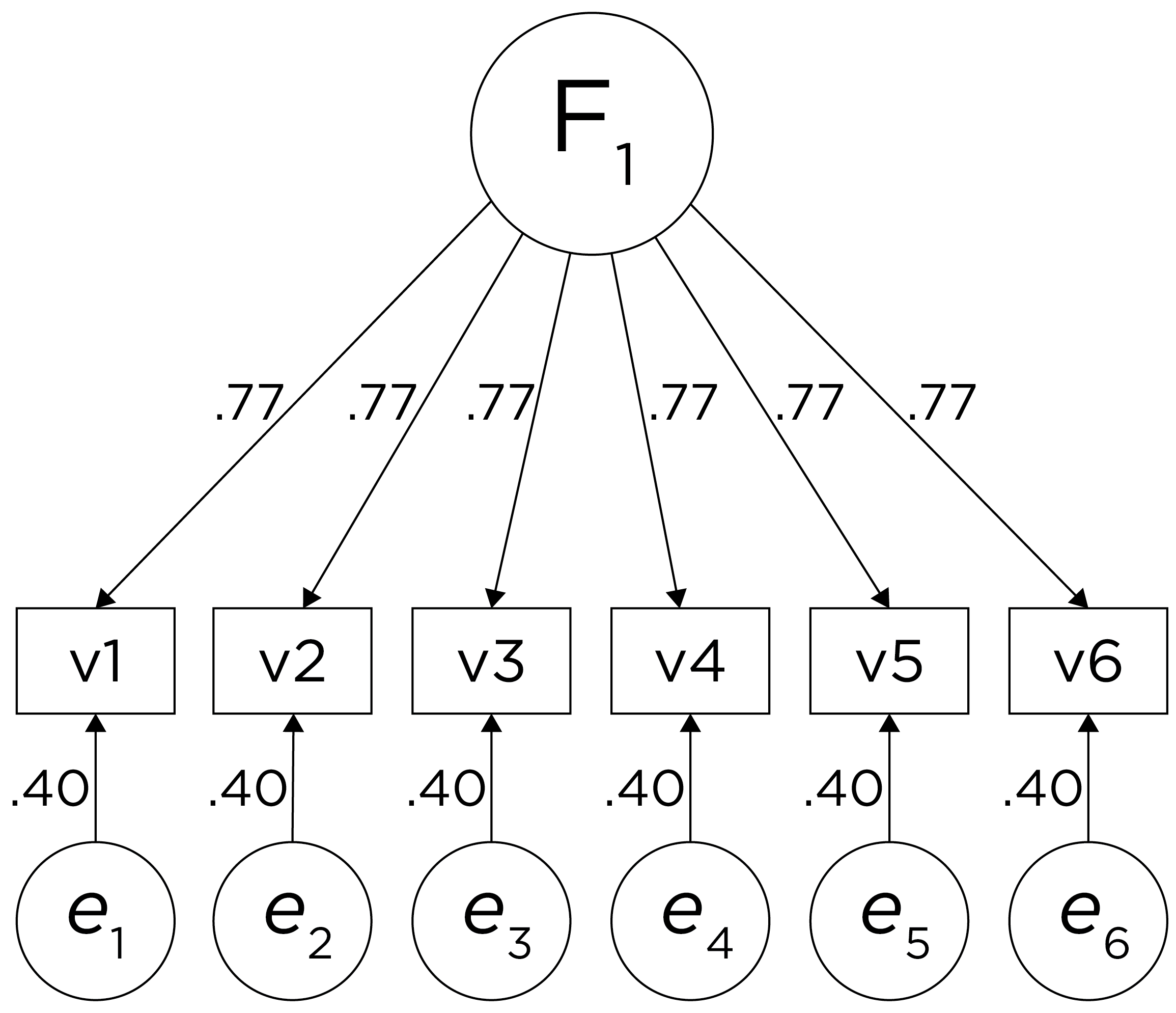
Figure 14.2: Example Confirmatory Factor Analysis Model: Unidimensional Model.
Consider a different correlation matrix in Figure 14.3. There is no common variance (correlations between the variables are zero), so there is no reason to believe there is a common factor that influences all of the variables. Variables that are not correlated cannot be related by a third variable, such as a common factor, so a common factor is not the right model.
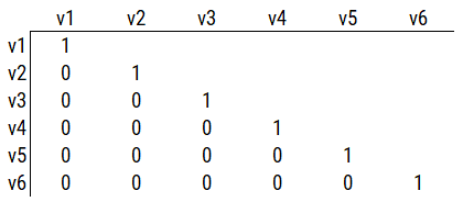
Figure 14.3: Example Correlation Matrix 2.
Consider another correlation matrix in Figure 14.4.
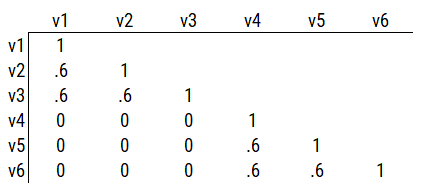
Figure 14.4: Example Correlation Matrix 3.
If you try to fit a single factor to this correlation matrix, it generates a factor model depicted in Figure 14.5. In this model, the first three variables have a factor loading of .77, but the remaining three variables have a factor loading of zero. This indicates that three remaining factors likely do not share a common factor with the first three variables.
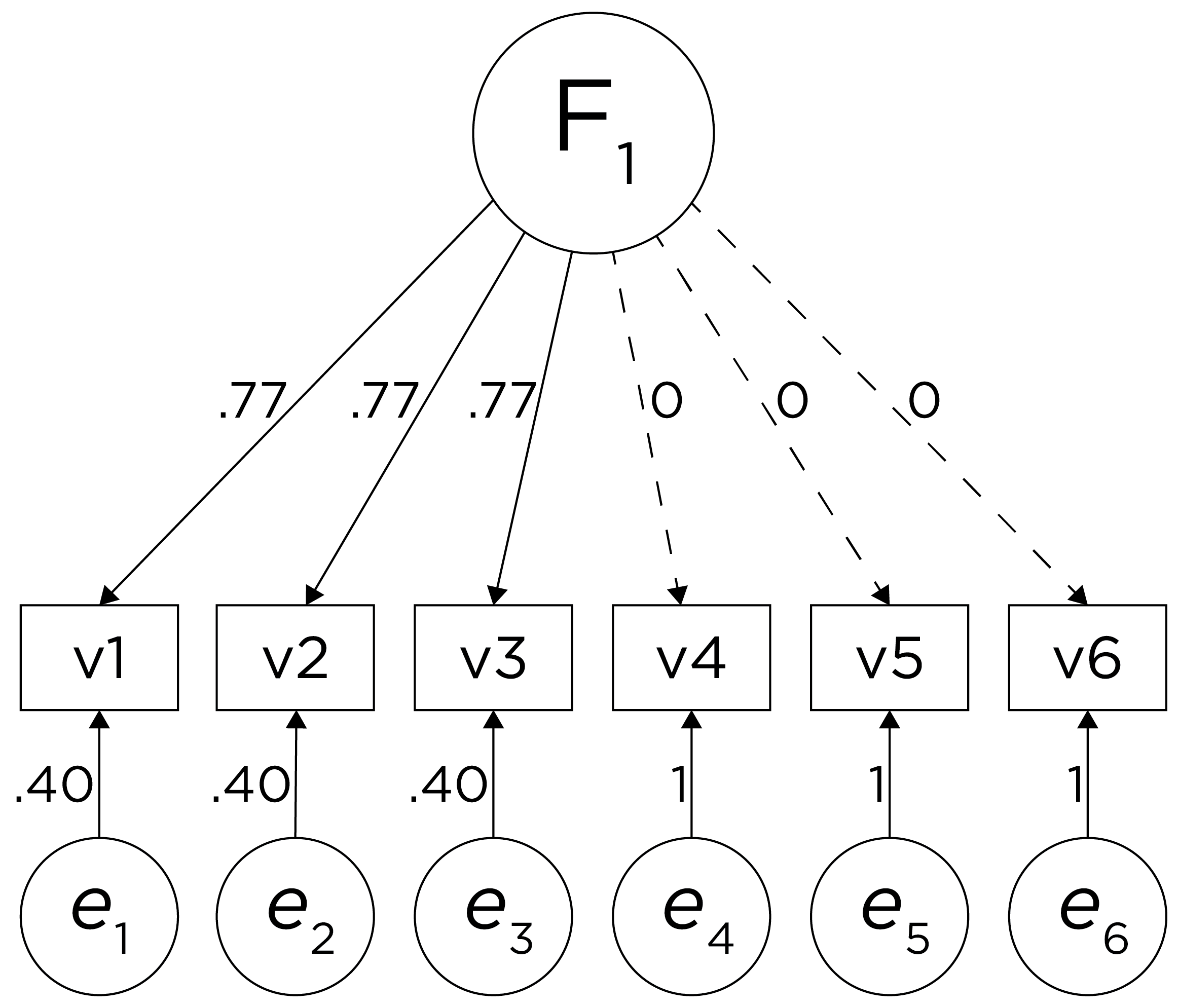
Figure 14.5: Example Confirmatory Factor Analysis Model: Multidimensional Model.
Therefore, a one-factor model is probably not correct; instead, the structure of the data is probably best represented by a two-factor model, as depicted in Figure 14.6. In the model, Factor 1 explains why measures 1, 2, and 3 are correlated, whereas Factor 2 explains why measures 4, 5, and 6 are correlated. A two-factor model thus explains why measures 1, 2, and 3 are not correlated with measures 4, 5, and 6. In this model, each latent factor accounts for 60% of the variance in the indicators that load onto it: \(\frac{.77^2 + .77^2 + .77^2}{3} = \frac{.60 + .60 + .60}{3} = .60\). Each latent factor accounts for 30% of the variance in all of the indicators: \(\frac{.77^2 + .77^2 + .77^2 + 0^2 + 0^2 + 0^2}{6} = \frac{.60 + .60 + .60 + 0 + 0 + 0}{6} = .30\).
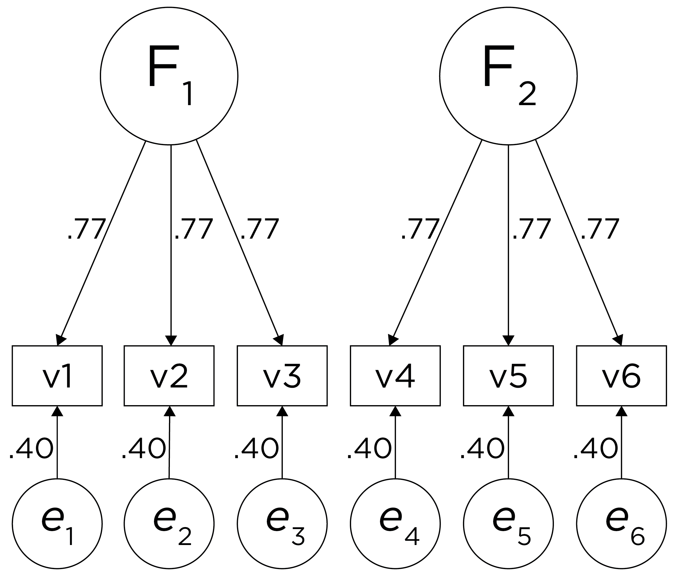
Figure 14.6: Example Confirmatory Factor Analysis Model: Two-Factor Model With Uncorrelated Factors.
Consider another correlation matrix in Figure 14.7.
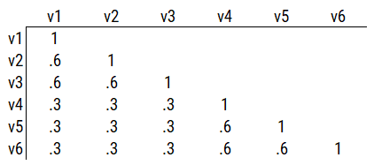
Figure 14.7: Example Correlation Matrix 4.
One way to model these data is depicted in Figure 14.8. In this model, the factor loadings are .77, the residual error terms are .40, and there is a covariance path of .50 for the association between Factor 1 and Factor 2. Going from the model to the correlation matrix is deterministic. If you know the model, you can calculate the correlation matrix. For instance, using path tracing rules (described in Section 4.1), the correlation of measures within a factor in this model is calculated as: \(0.60 = .77 \times .77\). Using path tracing rules, the correlation of measures across factors in this model is calculated as: \(.30 = .77 \times .50 \times .77\). In this model, each latent factor accounts for 60% of the variance in the indicators that load onto it: \(\frac{.77^2 + .77^2 + .77^2}{3} = \frac{.60 + .60 + .60}{3} = .60\). Each latent factor accounts for 37% of the variance in all of the indicators: \(\frac{.77^2 + .77^2 + .77^2 + (.50^2 \times .77^2) + (.50^2 \times .77^2) + (.50^2 \times .77^2)}{6} = \frac{.60 + .60 + .60 + .15 + .15 + .15}{6} = .37\).
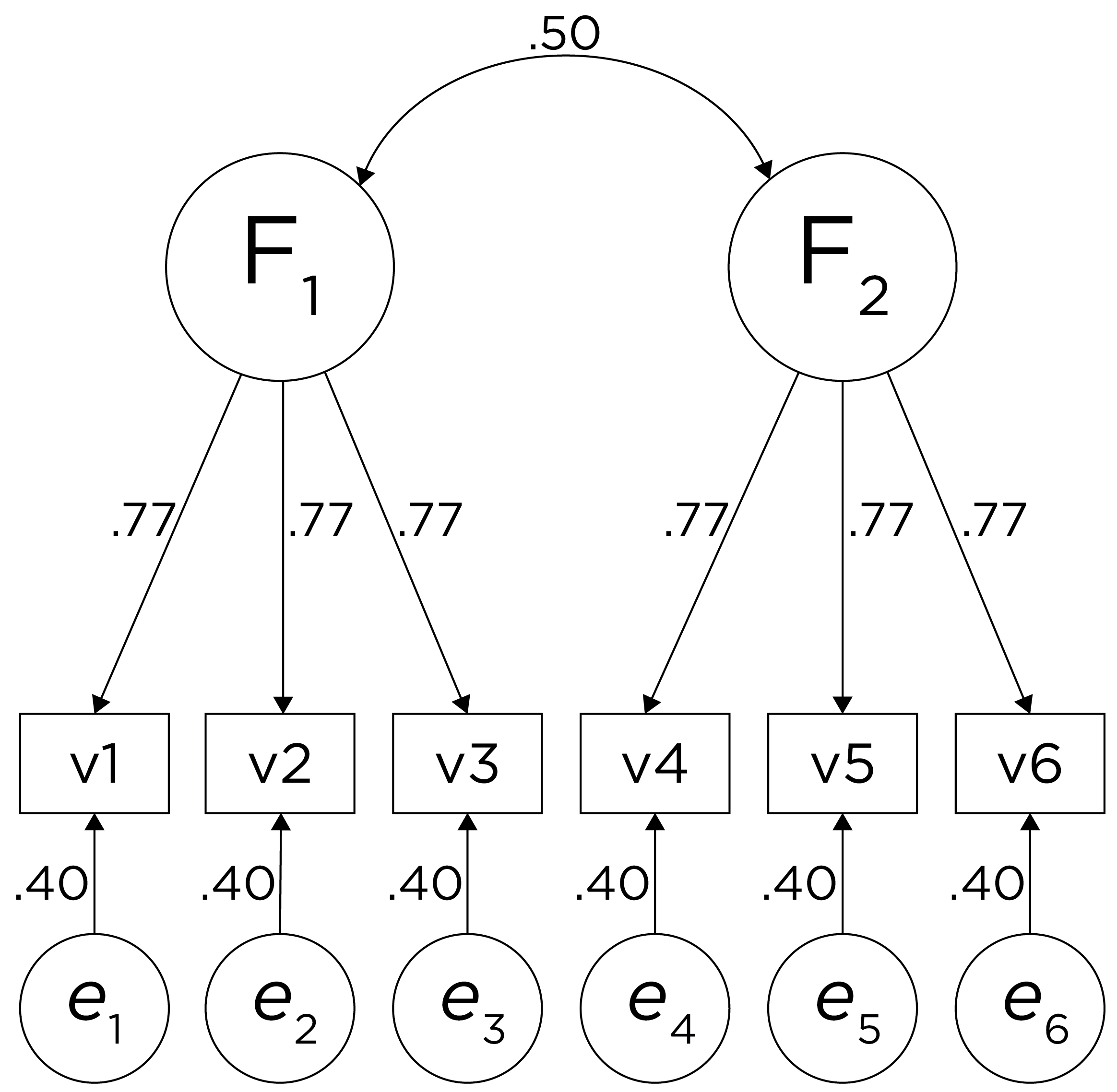
Figure 14.8: Example Confirmatory Factor Analysis Model: Two-Factor Model With Correlated Factors.
Although going from the model to the correlation matrix is deterministic, going from the correlation matrix to the model is not deterministic. If you know the correlation matrix, there may be many possible models. For instance, the model could also be the one depicted in Figure 14.9, with factor loadings of .77, residual error terms of .40, a regression path of .50, and a disturbance term of .75. The proportion of variance in Factor 2 that is explained by Factor 1 is calculated as: \(.25 = .50 \times .50\). The disturbance term is calculated as \(.75 = 1 - (.50 \times .50) = 1 - .25\). In this model, each latent factor accounts for 60% of the variance in the indicators that load onto it: \(\frac{.77^2 + .77^2 + .77^2}{3} = \frac{.60 + .60 + .60}{3} = .60\). Factor 1 accounts for 15% of the variance in the indicators that load onto Factor 2: \(\frac{(.50^2 \times .77^2) + (.50^2 \times .77^2) + (.50^2 \times .77^2)}{3} = \frac{.15 + .15 + .15}{3} = .15\). This model has the exact same fit as the previous model, but it has different implications. Unlike the previous model, in this model, there is a “causal” pathway from Factor 1 to Factor 2. However, the causal effect of Factor 1 does not account for all of the variance in Factor 2 because the correlation is only .50.
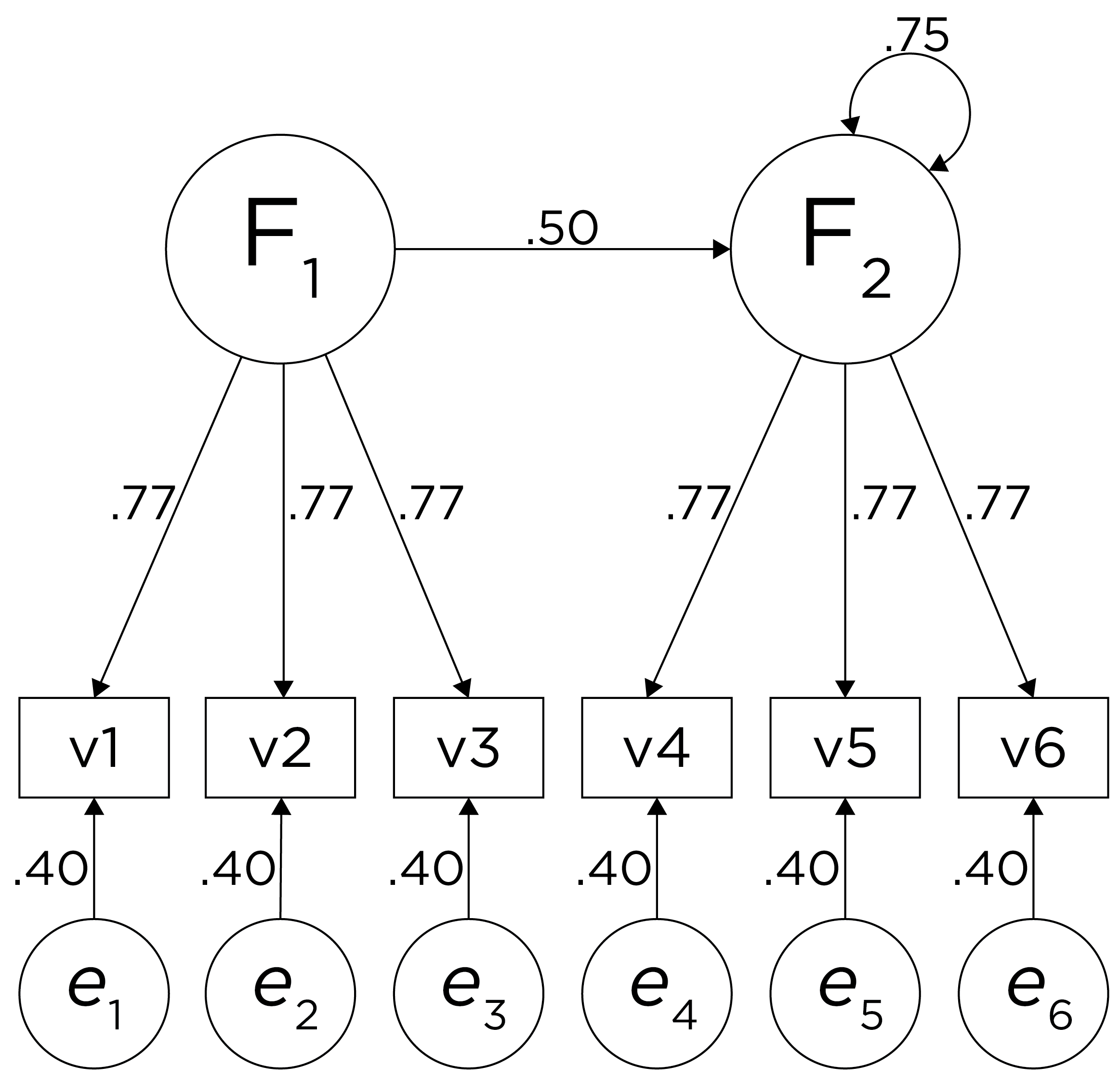
Figure 14.9: Example Confirmatory Factor Analysis Model: Two-Factor Model With Regression Path.
Alternatively, something else (e.g., another factor) could be explaining the data that we have not considered, as depicted in Figure 14.10. This is a higher-order factor model, in which there is a higher-order factor (\(A_1\)) that influences both lower-order factors, Factor 1 (\(F_1\)) and Factor 2 (\(F_2\)). The factor loadings from the lower order factors to the manifest variables are .77, the factor loading from the higher-order factor to the lower-order factors is .71, and the residual error terms are .40. This model has the exact same fit as the previous models. The proportion of variance in a lower-order factor (\(F_1\) or \(F_2\)) that is explained by the higher-order factor (\(A_1\)) is calculated as: \(.50 = .71 \times .71\). The disturbance term is calculated as \(.50 = 1 - (.71 \times .71) = 1 - .50\). Using path tracing rules, the correlation of measures across factors in this model is calculated as: \(.30 = .77 \times .71 \times .71 \times .77\). In this model, the higher-order factor (\(A_1\)) accounts for 30% of the variance in the indicators: \(\frac{(.77^2 \times .71^2) + (.77^2 \times .71^2) + (.77^2 \times .71^2) + (.77^2 \times .71^2) + (.77^2 \times .71^2) + (.77^2 \times .71^2)}{6} = \frac{.30 + .30 + .30 + .30 + .30 + .30}{6} = .30\).
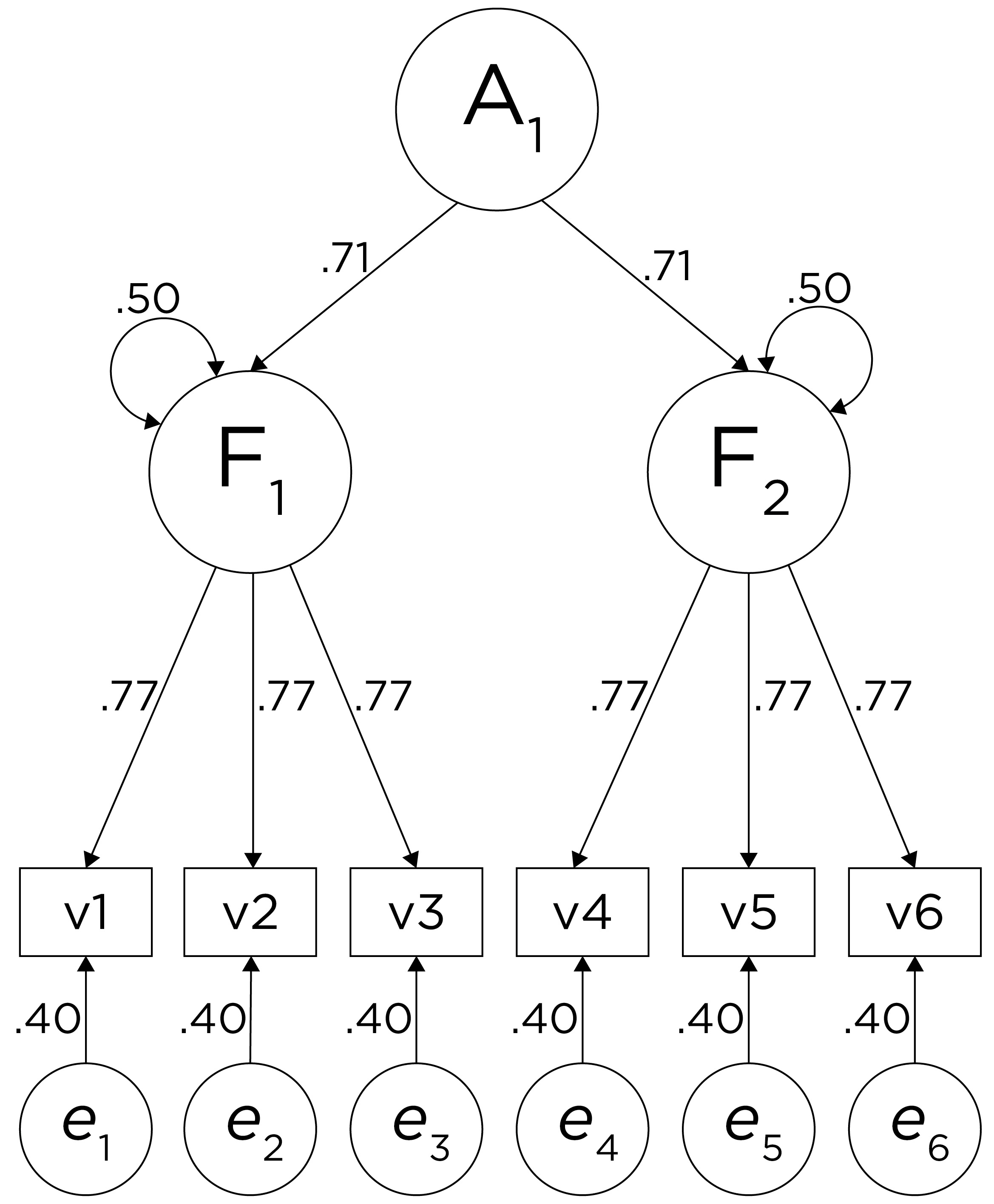
Figure 14.10: Example Confirmatory Factor Analysis Model: Higher-Order Factor Model.
Alternatively, there could be a single factor that ties measures 1, 2, and 3 together and measures 4, 5, and 6 together, as depicted in Figure 14.11. In this model, the measures no longer have merely random error: measures 1, 2, and 3 have correlated residuals—that is, they share error variance (i.e., systematic error); likewise, measures 4, 5, and 6 have correlated residuals. This model has the exact same fit as the previous models. The amount of common variance (\(R^2\)) that is accounted for by an indicator is estimated as the square of the standardized loading: \(.30 = .55 \times .55\). The amount of error for an indicator is estimated as: \(\text{error} = 1 - \text{common variance}\), so in this case, the amount of error is: \(.70 = 1 - .30\). Using path tracing rules, the correlation of measures within a factor in this model is calculated as: \(.60 = (.55 \times .55) + (.70 \times .43 \times .70) + (.70 \times .43 \times .43 \times .70)\). The correlation of measures across factors in this model is calculated as: \(.30 = .55 \times .55\). In this model, the latent factor accounts for 30% of the variance in the indicators: \(\frac{.55^2 + .55^2 + .55^2 + .55^2 + .55^2 + .55^2}{6} = \frac{.30 + .30 + .30 + .30 + .30 + .30}{6} = .30\).
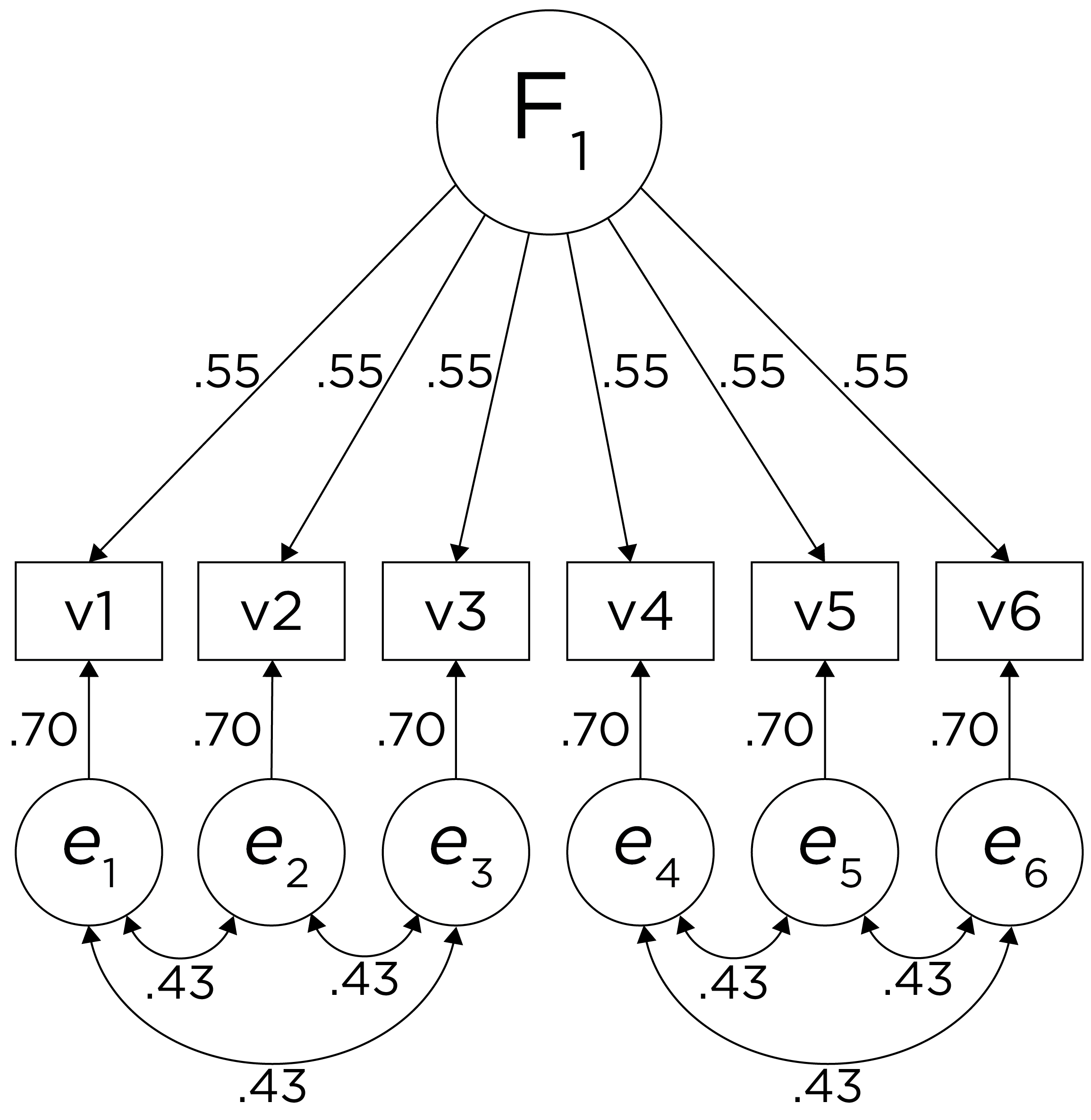
Figure 14.11: Example Confirmatory Factor Analysis Model: Unidimensional Model With Correlated Residuals.
Alternatively, there could be a single factor that influences measures 1, 2, 3, 4, 5, and 6 in addition to a method bias factor (e.g., a particular measurement method, item stem, reverse-worded item, or another method bias) that influences measures 4, 5, and 6 equally, as depicted in Figure 14.12. In this model, measures 4, 5, and 6 have cross-loadings—that is, they load onto more than one latent factor. This model has the exact same fit as the previous models. The amount of common variance (\(R^2\)) that is accounted for by an indicator is estimated as the sum of the squared standardized loadings: \(.60 = .77 \times .77 = (.39 \times .39) + (.67 \times .67)\). The amount of error for an indicator is estimated as: \(\text{error} = 1 - \text{common variance}\), so in this case, the amount of error is: \(.40 = 1 - .60\). Using path tracing rules, the correlation of measures within a factor in this model is calculated as: \(.60 = (.77 \times .77) = (.39 \times .39) + (.67 \times .67)\). The correlation of measures across factors in this model is calculated as: \(.30 = .77 \times .39\). In this model, the first latent factor accounts for 37% of the variance in the indicators: \(\frac{.77^2 + .77^2 + .77^2 + .39^2 + .39^2 + .39^2}{6} = \frac{.59 + .59 + .59 + .15 + .15 + .15}{6} = .30\). The second latent factor accounts for 45% of the variance in its indicators: \(\frac{.67^2 + .67^2 + .67^2}{3} = \frac{.45 + .45 + .45}{3} = .45\).
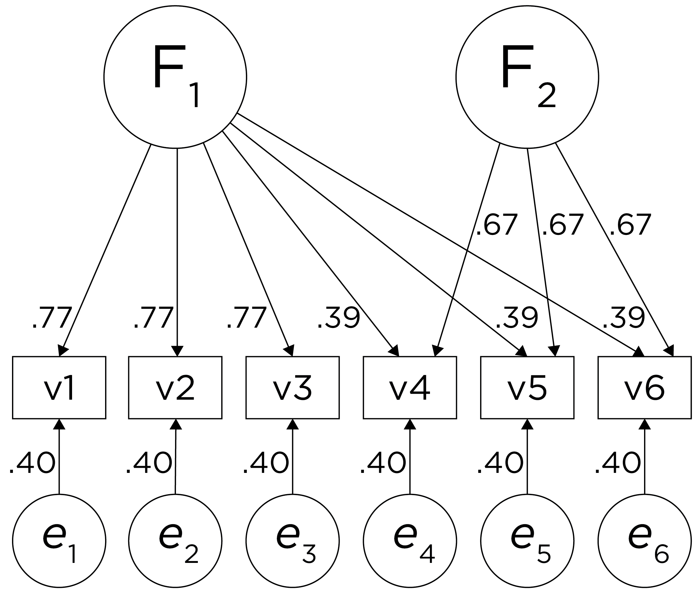
Figure 14.12: Example Confirmatory Factor Analysis Model: Two-Factor Model With Cross-Loadings.
14.1.2 Indeterminacy
There could be many more models that have the same fit to the data. Thus, factor analysis has indeterminacy because all of these models can explain these same data equally well, with all having different theoretical meaning. Factor indeterminacy reflects uncertainty (Rigdon et al., 2019a). The goal of factor analysis is for the model to look at the data and induce the model. However, most data matrices in real life are very complicated—much more complicated than in these examples.
This is why we do not calculate our own factor analysis by hand; use a stats program! It is important to think about the possibility of other models to determine how confident you can be in your data model. For every fully specified factor model—i.e., where the relevant paths are all defined, there is one and only one predictive data matrix (correlation matrix). However, each data matrix can produce many different factor models. Equivalent models are different models with the same degrees of freedom that have the same fit to the data. Rules for generating equivalent models are provided by S. Lee & Hershberger (1990). There is no way to distinguish which of these factor models is correct from the data matrix alone. Any given data matrix can predict an infinite number of factor models that accurately represent the data structure (Raykov & Marcoulides, 2001)—so we make decisions that determine what type of factor solution our data will yield. In general, factor indeterminacy—and the uncertainty it creates—tends to be greater in models with fewer items and where those items have smaller factor loadings and larger residual variances (Rigdon et al., 2019a). Conversely, factor indeterminacy is lower when there are many items per latent factor, and when loadings and factor correlations are strong (Rigdon et al., 2019b). Further, factor indeterminacy is compounded when creating factor scores for use in separate analyses [rather than estimating the associations within the same model; Rigdon et al. (2019a)]. Thus, where possible, it is preferable to estimate associations between factors and other variables within the same model.
Many models could explain your data, and there are many more models that do not explain the data. For equally good-fitting models, decide based on interpretability. If you have strong theory, decide based on theory and things outside of factor analysis!
14.1.3 Practical Considerations
There are important considerations for doing factor analysis in real life with complex data. Traditionally, researchers had to consider what kind of data they have, and they often assumed interval-level data even though data in psychology are often not interval data. In the past, factor analysis was not good with categorical and dichotomous (e.g., True/False) data because the variance then is largely determined by the mean. So, we need something more complicated for dichotomous data. More solutions are available now for factor analysis with ordinal and dichotomous data, but it is generally best to have at least four ordered categories to perform factor analysis.
The necessary sample size depends on the complexity of the true factor structure. If there is a strong single factor for 30 items, then \(N = 50\) is plenty. But if there are five factors and some correlated errors, then the sample size will need to be closer to ~5,000. Factor analysis can recover the truth when the world is simple. However, nature is often not simple, and it may end in the distortion of nature instead of nature itself.
Recommendations for factor analysis are described by Sellbom & Tellegen (2019).
14.1.4 Decisions to Make in Factor Analysis
There are many decisions to make in factor analysis (Floyd & Widaman, 1995; Sarstedt et al., 2024). These decisions can have important impacts on the resulting solution. Decisions include things such as:
- What variables to include in the model and how to scale them
- Method of factor extraction: factor analysis or PCA
- If factor analysis, the kind of factor analysis: EFA or CFA
- How many factors to retain
- If EFA or PCA, whether and how to rotate factors (factor rotation)
- Model selection and interpretation
14.1.4.1 1. Variables to Include and their Scaling
The first decision when conducting a factor analysis is which variables to include and the scaling of those variables. What factors (or components) you extract can differ widely depending on what variables you include in the analysis. For example, if you include many variables from the same source (e.g., self-report), it is possible that you will extract a factor that represents the common variance among the variables from that source (i.e., the self-reported variables). This would be considered a method factor, which works against the goal of estimating latent factors that represent the constructs of interest (as opposed to the measurement methods used to estimate those constructs).
An additional consideration is the scaling of the variables. Before performing a PCA, it is generally important to ensure that the variables included in the PCA are on the same scale. PCA seeks to identify components that explain variance in the data, so if the variables are not on the same scale, some variables may contribute considerably more variance than others. A common way of ensuring that variables are on the same scale is to standardize them using, for example, z-scores that have a mean of zero and standard deviation of one. By contrast, factor analysis can better accommodate variables that are on different scales.
14.1.4.2 2. Method of Factor Extraction
The second decision is to select the method of factor extraction. This is the algorithm that is going to try to identify factors. There are two main families of factor or component extraction: analytic or principal components. The principal components approach is called principal component analysis (PCA). PCA is not really a form factor analysis; rather, it is useful for data reduction (Lilienfeld et al., 2015). The analytic family includes factor analysis approaches such as principal axis factoring and maximum likelihood factor analysis. The distinction between factor analysis and PCA is depicted in Figure 14.13.
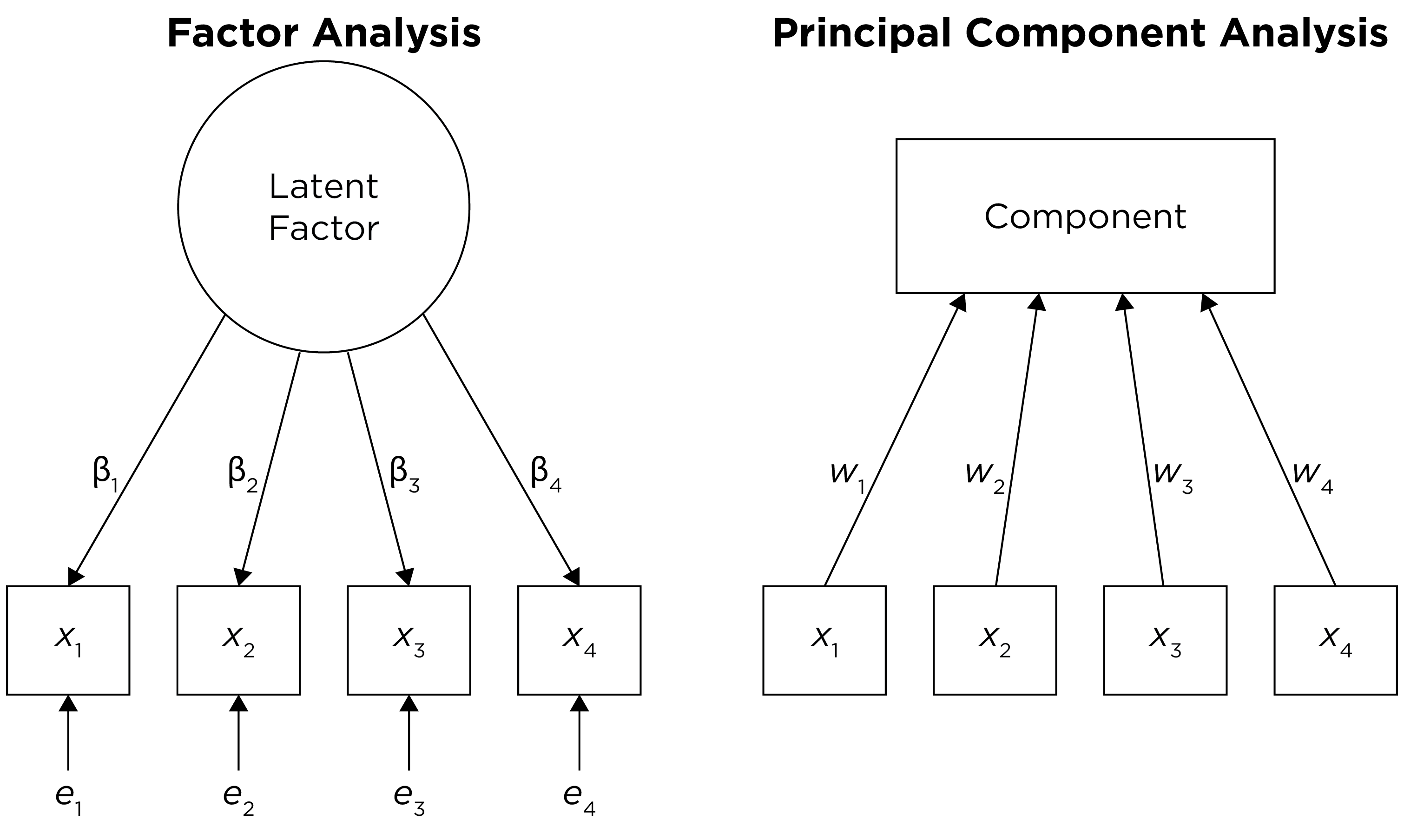
Figure 14.13: Distinction Between Factor Analysis and Principal Component Analysis.
14.1.4.2.1 Principal Component Analysis
Principal component analysis (PCA) is used if you want to reduce your data matrix. PCA composites represent the variances of an observed measure in as economical a fashion as possible, with no latent underlying variables. The goal of PCA is to identify a smaller number of components that explain as much variance in a set of variables as possible. It is an atheoretical way to decompose a matrix. PCA involves decomposition of a data matrix into a set of eigenvectors, which are transformations of the old variables.
The eigenvectors attempt to simplify the data in the matrix. PCA takes the data matrix and identifies the weighted sum of all variables that does the best job at explaining variance: these are the principal components, also called eigenvectors. Principal components reflect optimally weighted sums. In this way, PCA is a formative model (by contrast, factor analysis applies a reflective model).
PCA decomposes the data matrix into any number of components—as many as the number of variables, which will always account for all variance. After the model is fit, you can look at the results and discard the components which likely reflect error variance. Judgments about which factors to retain are based on empirical criteria in conjunction with theory to select a parsimonious number of components that account for the majority of variance.
The eigenvalue reflects the amount of variance explained by the component (eigenvector). When using a varimax (orthogonal) rotation, an eigenvalue for a component is calculated as the sum of squared standardized component loadings on that component. When using oblique rotation, however, the items explain more variance than is attributable to their factor loadings because the factors are correlated.
PCA pulls the first principal component out (i.e., the eigenvector that explains the most variance) and makes a new data matrix: i.e., new correlation matrix. Then the PCA pulls out the component that explains the next most variance—i.e., the eigenvector with the next largest eigenvalue, and it does this for all components, equal to the same number of variables. For instance, if there are six variables, it will iteratively extract an additional component up to six components. You can extract as many eigenvectors as there are variables. If you extract all six components, the data matrix left over will be the same as the correlation matrix in Figure 14.3. That is, the remaining variables (as part of the leftover data matrix) will be entirely uncorrelated with each other, because six components explain 100% of the variance from six variables. In other words, you can explain (6) variables with (6) new things!
However, it does no good if you have to use all (6) components because there is no data reduction from the original number of variables. When the goal is data reduction (as in PCA), the hope is that the first few components will explain most of the variance, so we can explain the variability in the data with fewer components than there are variables.
The sum of all eigenvalues is equal to the number of variables in the analysis. PCA does not have the same assumptions as factor analysis, which assumes that measures are partly from common variance and error. But if you estimate (6) eigenvectors and only keep (2), the model is a two-component model and whatever left becomes error. Therefore, PCA does not have the same assumptions as factor analysis, but it often ends up in the same place.
Most people who want to conduct a factor analysis use PCA, but PCA is not really factor analysis (Lilienfeld et al., 2015). PCA is what SPSS can do quickly. But computers are so fast now—just do a real factor analysis! Factor analysis better handles error than PCA—factor analysis assumes that what is in the variable is the combination of common construct variance and error. By contrast, PCA assumes that the measures have no measurement error.
14.1.4.2.2 Factor Analysis
Factor analysis is an analytic approach to factor extraction. Factor analysis is a special case of structural equation modeling (SEM). Factor analysis is an analytic technique that is interested in the factor structure of a measure or set of measures. Factor analysis is a theoretical approach that considers that there are latent theoretical constructs that influence the scores on particular variables. It assumes that part of the explanation for each variable is shared between variables (i.e., common variance), and that part of it is unique variance. The unique variance is considered error. In reality, part of the unique variance is random error and part of it is specific variance—systematic variance unique to the item, which may reflect either a unique facet of the construct or systematic error such as method bias that is specific to the item. The portion of common variance in an item (i.e., the portion of variance that is shared with other variables) is called communality, which is the proportion of the item’s variance that is explained by the latent factors (i.e., the \(R^2\) of an item). In factor analysis and PCA, communality of an item is estimated as the sum of squared standardized loadings for an item across all retained factors/components. The average variance extracted (AVE) is a factor-level index that represents the average communality across all items that load on a given factor. For an individual item, the unique variance (error + specific variance) is: \(1 - \text{communality}\). The common variance is thought to be a purer estimate of the latent construct than the total variance of the item, which includes error variance. However, the common variance includes all variance that is shared across all variables, including construct variance (i.e., true score variance) and systematic error such as method bias.
There are several types of factor analysis, including principal axis factoring and maximum likelihood factor analysis. Factor analysis can be used to test measurement/factorial invariance and for multitrait-multimethod designs. One example of a MTMM model in factor analysis is the correlated traits correlated methods model (Tackett, Lang, et al., 2019).
There are several differences between (real) factor analysis versus PCA. Factor analysis has greater sophistication than PCA, but greater sophistication often results in greater assumptions. Factor analysis does not always work; the data may not always fit to a factor analysis model; therefore, use PCA as a second/last option. PCA can decompose any data matrix; it always works. PCA is okay if you are not interested in the factor structure. PCA uses all variance of variables and assumes variables have no error, so it does not account for measurement error. PCA is good if you just want to form a linear composite and if the causal structure is formative (rather than reflective). However, if you are interested in the factor structure, use factor analysis, which estimates a latent variable that accounts for the common variance and discards error variance. Factor analysis is useful for the identification of latent constructs—i.e., underlying dimensions or factors that explain (cause) scores on items.
14.1.4.3 3. EFA or CFA
A third decision is the kind of factor analysis to use: exploratory factor analysis (EFA) or confirmatory factor analysis (CFA).
14.1.4.3.1 Exploratory Factor Analysis (EFA)
Exploratory factor analysis (EFA) is used if you have no a priori hypotheses about the factor structure of the model, but you would like to understand the latent variables represented by your items.
EFA is partly induced from the data. You feed in the data and let the program build the factor model. You can set some parameters going in, including how to extract or rotate the factors. The factors are extracted from the data without specifying the number and pattern of loadings between the items and the latent factors (Bollen, 2002). All cross-loadings are freely estimated.
14.1.4.3.2 Confirmatory Factor Analysis (CFA)
Confirmatory factor analysis (CFA) is used to (dis)confirm a priori hypotheses about the factor structure of the model. CFA is a test of the hypothesis. In CFA, you specify the model and ask how well this model represents the data. The researcher specifies the number, meaning, associations, and pattern of free parameters in the factor loading matrix (Bollen, 2002). A key advantage of CFA is the ability to directly compare alternative models (i.e., factor structures), which is valuable for theory testing (Strauss & Smith, 2009). For instance, you could use CFA to test whether the variance in several measures’ scores is best explained with one factor or two factors. In CFA, cross-loadings are not estimated unless the researcher specifies them.
14.1.4.3.3 Exploratory Structural Equation Modeling (ESEM)
In real life, there is not a clear distinction between EFA and CFA. In CFA, researchers often set only half of the constraints, and let the data fill in the rest. Moreover, our initial hypothesized CFA model is often not a good fit to the data—especially for models with many items (Floyd & Widaman, 1995)—and requires modification for adequate fit, such as cross loadings and correlated residuals. Such modifications are often made based on empirical criteria (e.g., modification indices) rather than our initial hypothesis. In EFA, researchers often set constraints and assumptions. Moreover, the initial items for the EFA were selected by the researcher, who often has expectations about the number and types of factors that will be extracted. Thus, the line between EFA and CFA is often blurred. There is an exploratory–confirmatory continuum, and the important thing is to report which aspects of your modeling approach were exploratory and which were confirmatory.
EFA and CFA can be considered special cases of exploratory structural equation modeling (ESEM), which combines features of EFA, CFA, and SEM (Marsh et al., 2014). ESEM can include any combination of exploratory (i.e., EFA) and confirmatory (CFA) factors. ESEM, unlike traditional CFA models, typically estimates all cross-loadings—at least for the exploratory factors. If a CFA model without cross-loadings and correlated residuals fits as well as an ESEM model with all cross-loadings, the CFA model should be retained for its simplicity. However, ESEM models often fit better than CFA models because requiring no cross-loadings is an unrealistic expectation of items from many psychological instruments (Marsh et al., 2014). The correlations between factors tend to be positively biased when fitting CFA models without cross-loadings, which leads to challenges in using CFA to establish discriminant validity (Marsh et al., 2014). Thus, compared to CFA, ESEM has the potential to more accurately estimate factor correlations and establish discriminant validity (Marsh et al., 2014). Moreover, ESEM can be useful in a multitrait-multimethod framework. We provide examples of ESEM in Section 14.4.3.
14.1.4.4 4. How Many Factors to Retain
A goal of factor analysis and PCA is simplification or parsimony, while still explaining as much variance as possible. The hope is that you can have fewer factors that explain the associations between the variables than the number of observed variables. The fewer the number of factors retained, the greater the parsimony, but the greater the amount of information that is discarded (i.e., the less the variance accounted for in the variables). The more factors we retain, the less the amount of information that is discarded (i.e., more variance is accounted for in the variables), but the less the parsimony. But how do you decide on the number of factors (in factor analysis) or components (in PCA)?
There are a number of criteria that one can use to help determine how many factors/components to keep:
- Kaiser-Guttman criterion (Kaiser, 1960): in PCA, components with eigenvalues greater than 1
- or, for factor analysis, factors with eigenvalues greater than zero
- Cattell’s scree test (Cattell, 1966): the “elbow” (inflection point) in a scree plot minus one; sometimes operationalized with optimal coordinates (OC) or the acceleration factor (AF)
- Parallel analysis: factors that explain more variance than randomly simulated data
- Very simple structure (VSS) criterion: larger is better
- Velicer’s minimum average partial (MAP) test: smaller is better
- Akaike information criterion (AIC): smaller is better
- Bayesian information criterion (BIC): smaller is better
- Sample size-adjusted BIC (SABIC): smaller is better
- Root mean square error of approximation (RMSEA): smaller is better
- Chi-square difference test: smaller is better; a significant test indicates that the more complex model is significantly better fitting than the less complex model
- Standardized root mean square residual (SRMR): smaller is better
- Comparative Fit Index (CFI): larger is better
- Tucker Lewis Index (TLI): larger is better
There is not necessarily a “correct” criterion to use in determining how many factors to keep, so it is generally recommended that researchers use multiple criteria in combination with theory and interpretability.
A scree plot from a factor analysis or PCA provides lots of information. A scree plot has the factor number on the x-axis and the eigenvalue on the y-axis. The eigenvalue is the variance accounted for by a factor; when using a varimax (orthogonal) rotation, an eigenvalue (or factor variance) is calculated as the sum of squared standardized factor (or component) loadings on that factor. An example of a scree plot is in Figure 14.14.
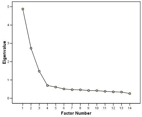
Figure 14.14: Example of a Scree Plot.
The total variance is equal to the number of variables you have, so one eigenvalue is approximately one variable’s worth of variance. In a factor analysis and PCA, the first factor (or component) accounts for the most variance, the second factor accounts for the second-most variance, and so on. The more factors you add, the less variance is explained by the additional factor.
One criterion for how many factors to keep is the Kaiser-Guttman criterion. According to the Kaiser-Guttman criterion (Kaiser, 1960), you should keep any factors whose eigenvalue is greater than 1. That is, for the sake of simplicity, parsimony, and data reduction, you should take any factors that explain more than a single variable would explain. According to the Kaiser-Guttman criterion, we would keep three factors from Figure 14.14 that have eigenvalues greater than 1. The default in SPSS is to retain factors with eigenvalues greater than 1. However, keeping factors whose eigenvalue is greater than 1 is not the most correct rule. If you let SPSS do this, you may get many factors with eigenvalues around 1 (e.g., factors with an eigenvalue ~ 1.0001) that are not adding so much that it is worth the added complexity. The Kaiser-Guttman criterion usually results in keeping too many factors. Factors with small eigenvalues around 1 could reflect error shared across variables. For instance, factors with small eigenvalues could reflect method variance (i.e., method factor), such as a self-report factor that turns up as a factor in factor analysis, but that may be useless to you as a conceptual factor of a construct of interest.
Another criterion is Cattell’s scree test (Cattell, 1966), which involves selecting the number of factors from looking at the scree plot. “Scree” refers to the rubble of stones at the bottom of a mountain. According to Cattell’s scree test, you should keep the factors before the last steep drop in eigenvalues—i.e., the factors before the rubble, where the slope approaches zero. The beginning of the scree (or rubble), where the slope approaches zero, is called the “elbow” of a scree plot. Using Cattell’s scree test, you retain the number of factors that explain the most variance prior to the explained variance drop-off, because, ultimately, you want to include only as many factors in which you gain substantially more by the inclusion of these factors. That is, you would keep the number of factors at the elbow of the scree plot minus one. If the last steep drop occurs from Factor 4 to Factor 5 and the elbow is at Factor 5, we would keep four factors. In Figure 14.14, the last steep drop in eigenvalues occurs from Factor 3 to Factor 4; the elbow of the scree plot occurs at Factor 4. We would keep the number of factors at the elbow minus one. Thus, using Cattell’s scree test, we would keep three factors based on Figure 14.14.
There are more sophisticated ways of using a scree plot, but they usually end up at a similar decision. Examples of more sophisticated tests include parallel analysis and very simple structure (VSS) plots. In a parallel analysis, you examine where the eigenvalues from observed data and random data converge, so you do not retain a factor that explains less variance than would be expected by random chance. A parallel analysis can be helpful when you have many variables and one factor accounts for the majority of the variance such that the elbow is at Factor 2 (which would result in keeping one factor), but you have theoretical reasons to select more than one factor. An example in which parallel analysis may be helpful is with neurophysiological data. For instance, parallel analysis can be helpful when conducting temporo-spatial PCA of event-related potential (ERP) data in which you want to separate multiple time windows and multiple spatial locations despite a predominant signal during a given time window and spatial location (Dien, 2012).
In general, my recommendation is to use Cattell’s scree test, and then test the factor solutions with plus or minus one factor. You should never accept PCA components with eigenvalues less than one (or factors with eigenvalues less than zero), because they are likely to be largely composed of error. If you are using maximum likelihood factor analysis, you can compare the fit of various models with model fit criteria to see which model fits best for its parsimony. A model will always fit better when you add additional parameters or factors, so you examine if there is significant improvement in model fit when adding the additional factor—that is, we keep adding complexity until additional complexity does not buy us much. Always try a factor solution that is one less and one more than suggested by Cattell’s scree test to buffer your final solution because the purpose of factor analysis is to explain things and to have interpretability. Even if all rules or indicators suggest to keep X number of factors, maybe \(\pm\) one factor helps clarify things. Even though factor analysis is empirical, theory and interpretatability should also inform decisions.
14.1.4.5 5. Factor Rotation
The next step if using EFA or PCA is, possibly, to rotate the factors to make them more interpretable and simple, which is the whole goal. To interpret the results of a factor analysis, we examine the factor matrix. The columns refer to the different factors; the rows refer to the different observed variables. The cells in the table are the factor loadings—they are basically the correlation between the variable and the factor. Our goal is to achieve a model with simple structure because it is easily interpretable. Simple structure means that every variable loads perfectly on one and only one factor, as operationalized by a matrix of factor loadings with values of one and zero and nothing else. An example of a factor matrix that follows simple structure is depicted in Figure 14.15.
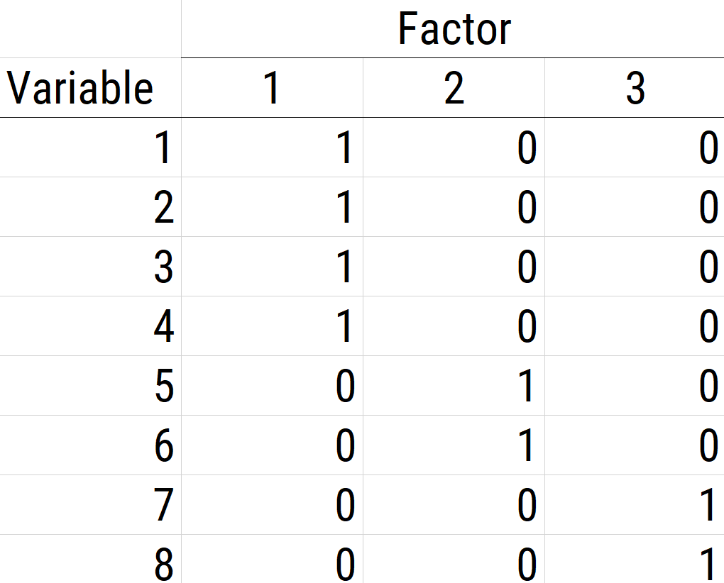
Figure 14.15: Example of a Factor Matrix That Follows Simple Structure.
An example of a measurement model that follows simple structure is depicted in Figure 14.16. Each variable loads onto one and only one factor, which makes it easy to interpret the meaning of each factor, because a given factor represents the common variance among the items that load onto it.
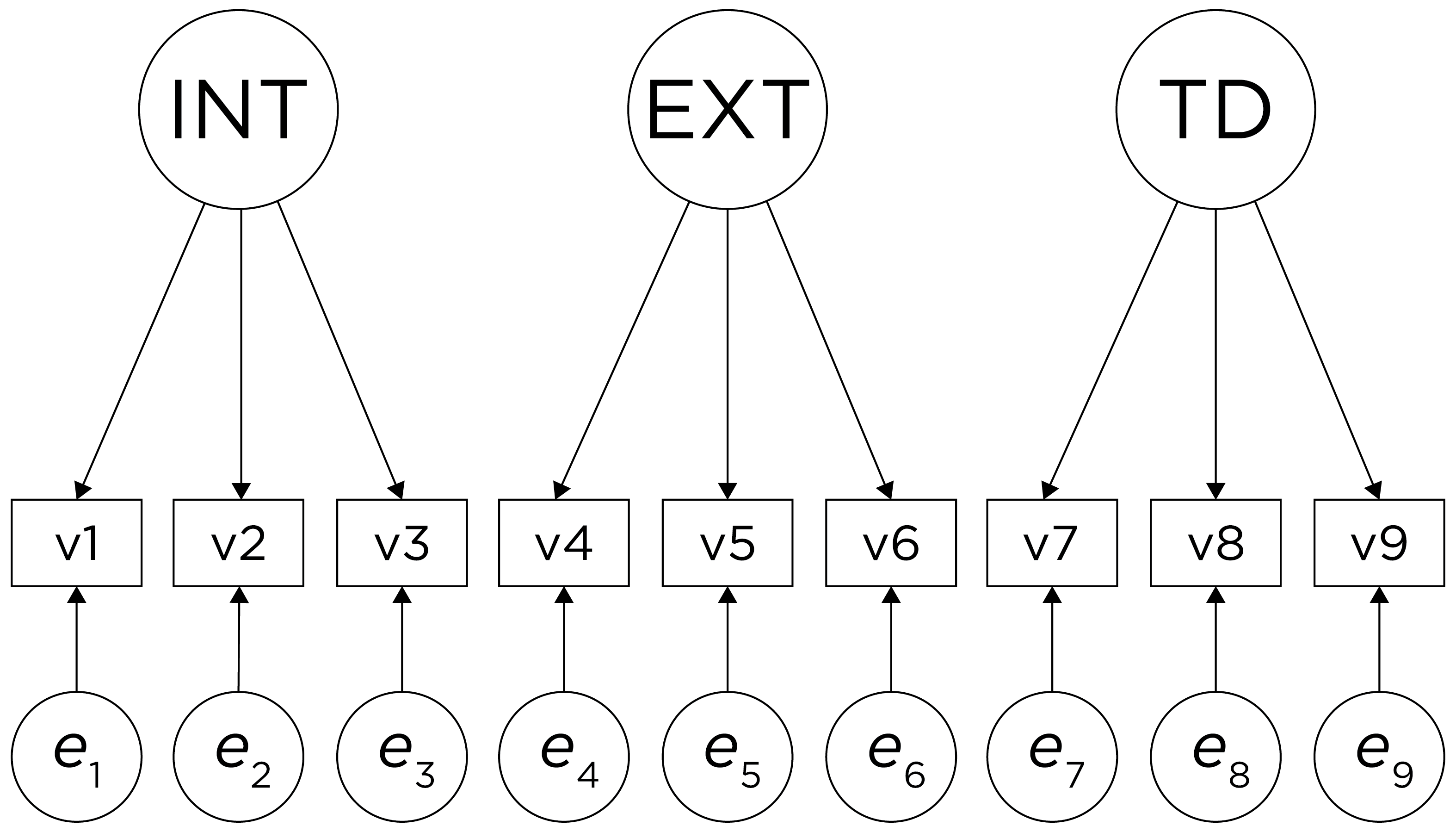
Figure 14.16: Example of a Measurement Model That Follows Simple Structure. ‘INT’ = internalizing problems; ‘EXT’ = externalizing problems; ‘TD’ = thought-disordered problems.
However, pure simple structure only occurs in simulations, not in real-life data. In reality, our measurement model in an unrotated factor analysis model might look like the model in Figure 14.17. In this example, the measurement model does not show simple structure because the items have cross-loadings—that is, the items load onto more than one factor. The cross-loadings make it difficult to interpret the factors, because all of the items load onto all of the factors, so the factors are not very distinct from each other, which makes it difficult to interpret what the factors mean.
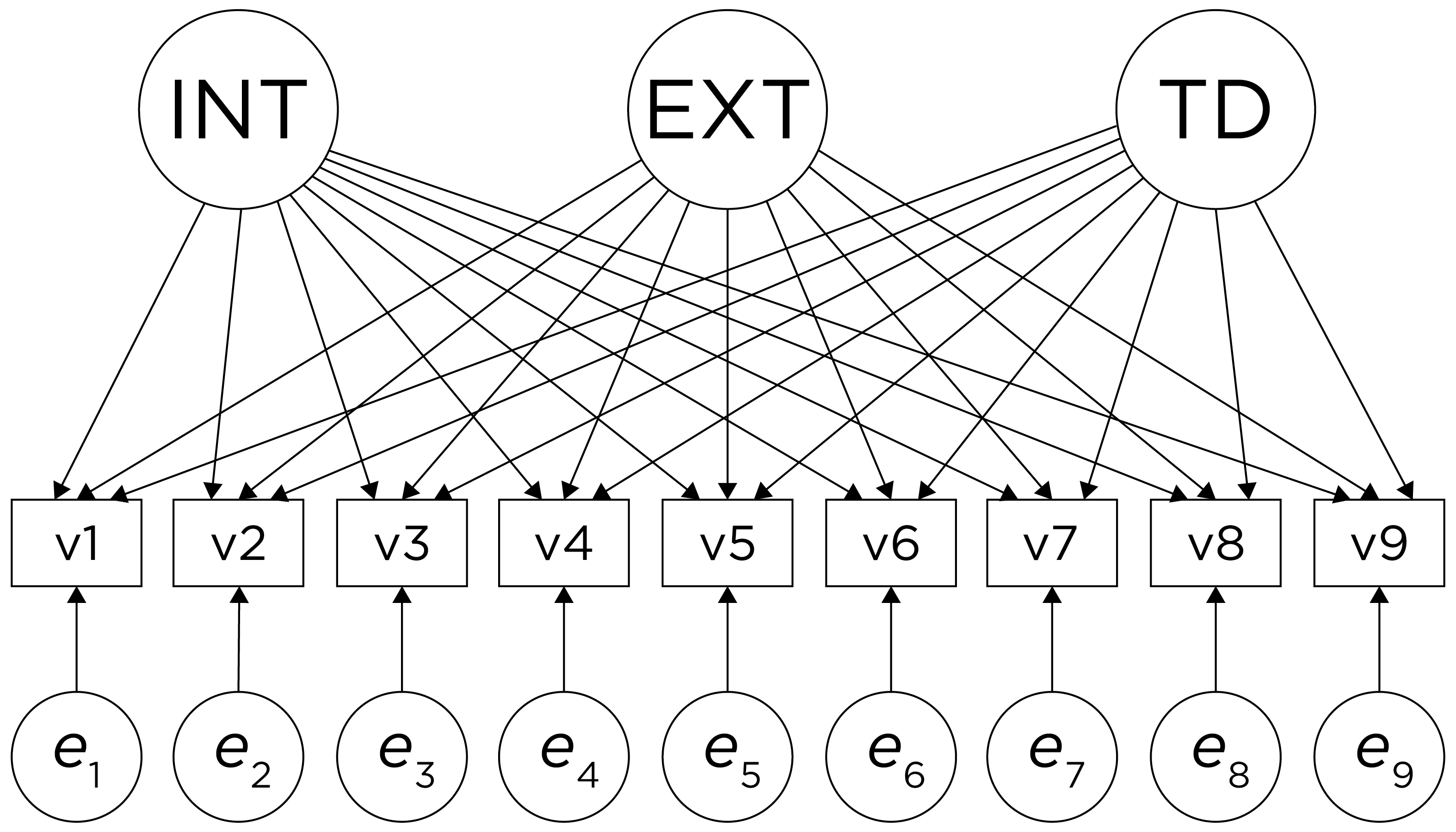
Figure 14.17: Example of a Measurement Model That Does Not Follow Simple Structure. ‘INT’ = internalizing problems; ‘EXT’ = externalizing problems; ‘TD’ = thought-disordered problems.
As a result of the challenges of interpretability caused by cross-loadings, factor rotations are often performed. An example of an unrotated factor matrix is in Figure 14.18.
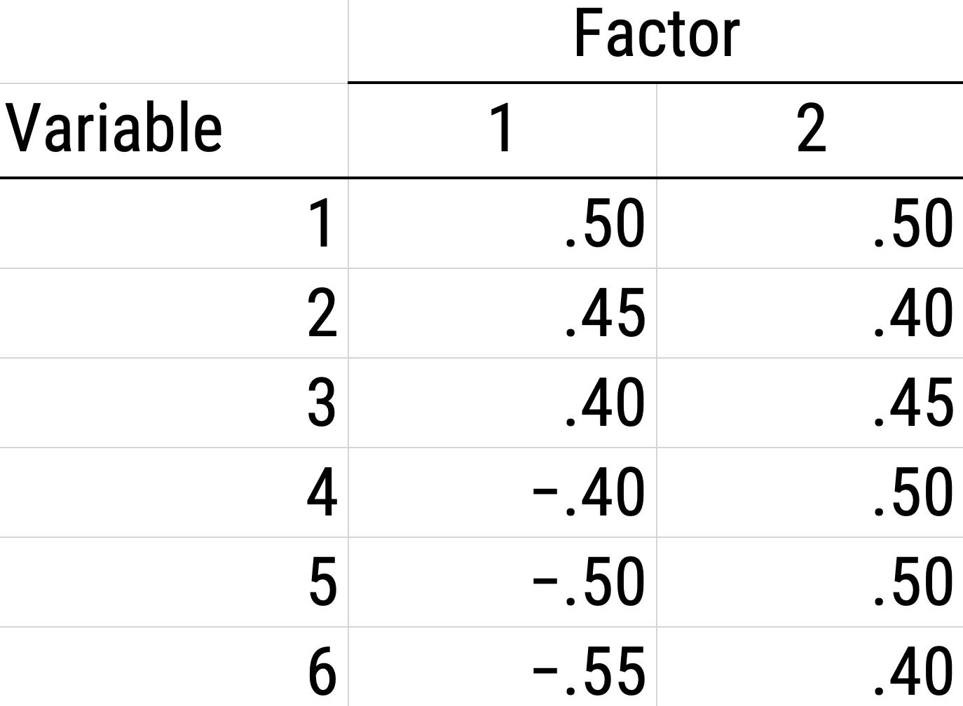
Figure 14.18: Example of a Factor Matrix.
In the example factor matrix in Figure 14.18, the factor analysis is not very helpful—it tells us very little because it did not distinguish between the two factors. The variables have similar loadings on Factor 1 and Factor 2. An example of a unrotated factor solution is in Figure 14.19. In the figure, all of the variables are in the midst of the quadrants—they are not on the factors’ axes. Thus, the factors are not very informative.
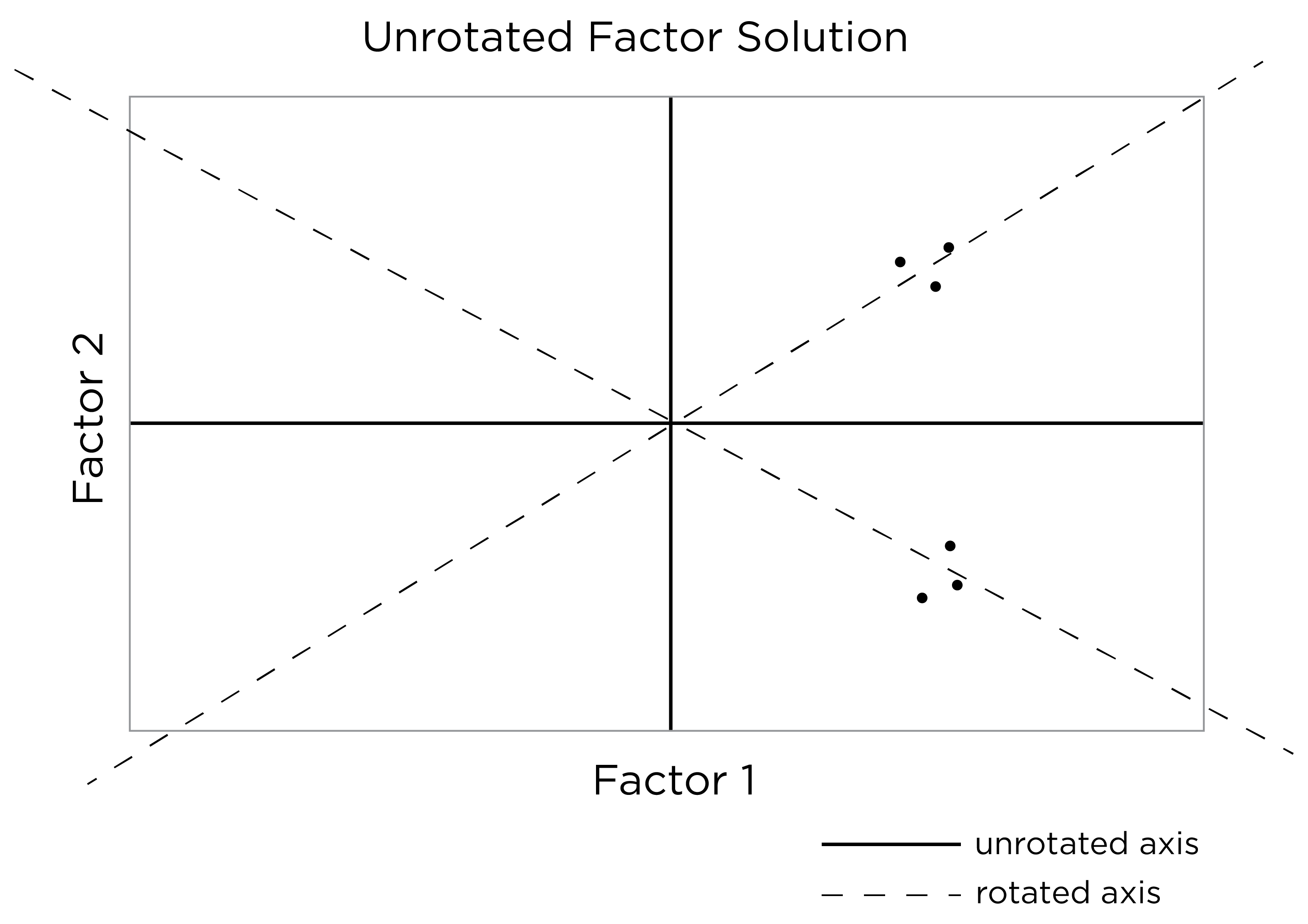
Figure 14.19: Example of an Unrotated Factor Solution.
As a result, to improve the interpretability of the factor analysis, we can do what is called rotation. Rotation leverages the idea that there are infinite solutions to the factor analysis model that fit equally well. Rotation involves changing the orientation of the factors by changing the axes so that variables end up with very high (close to one or negative one) or very low (close to zero) loadings, so that it is clear which factors include which variables (and which factors each variable most strongly loads onto). That is, rotation rescales the factors and tries to identify the ideal solution (factor) for each variable. Rotation occurs by changing the variables’ loadings while keeping the structure of correlations among the variables intact (Field et al., 2012). Moreover, rotation does not change the variance explained by factors. Rotation searches for simple structure and keeps searching until it finds a minimum (i.e., the closest as possible to simple structure). After rotation, if the rotation was successful for imposing simple structure, each factor will have loadings close to one (or negative one) for some variables and close to zero for other variables. The goal of factor rotation is to achieve simple structure, to help make it easier to interpret the meaning of the factors.
To perform factor rotation, orthogonal rotations are often used. Orthogonal rotations make the rotated factors uncorrelated. An example of a commonly used orthogonal rotation is varimax rotation. Varimax rotation maximizes the sum of the variance of the squared loadings (i.e., so that items have either a very high or very low loading on a factor) and yields axes with a 90-degree angle.
An example of a factor matrix following an orthogonal rotation is depicted in Figure 14.20. An example of a factor solution following an orthogonal rotation is depicted in Figure 14.21.
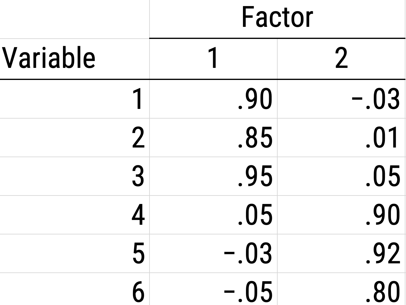
Figure 14.20: Example of a Rotated Factor Matrix.
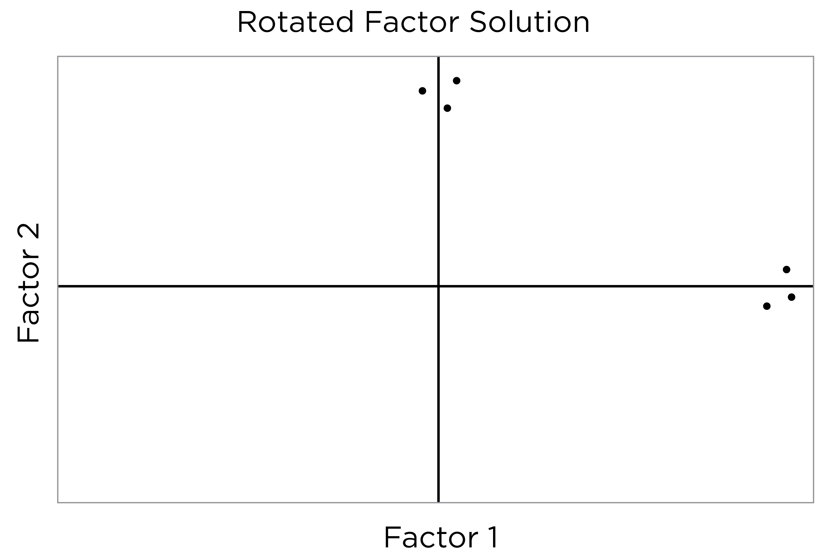
Figure 14.21: Example of a Rotated Factor Solution.
An example of a factor matrix from SPSS following an orthogonal rotation is depicted in Figure 14.22.
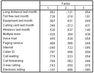
Figure 14.22: Example of a Rotated Factor Matrix From SPSS.
An example of a factor structure from an orthogonal rotation is in Figure 14.23.
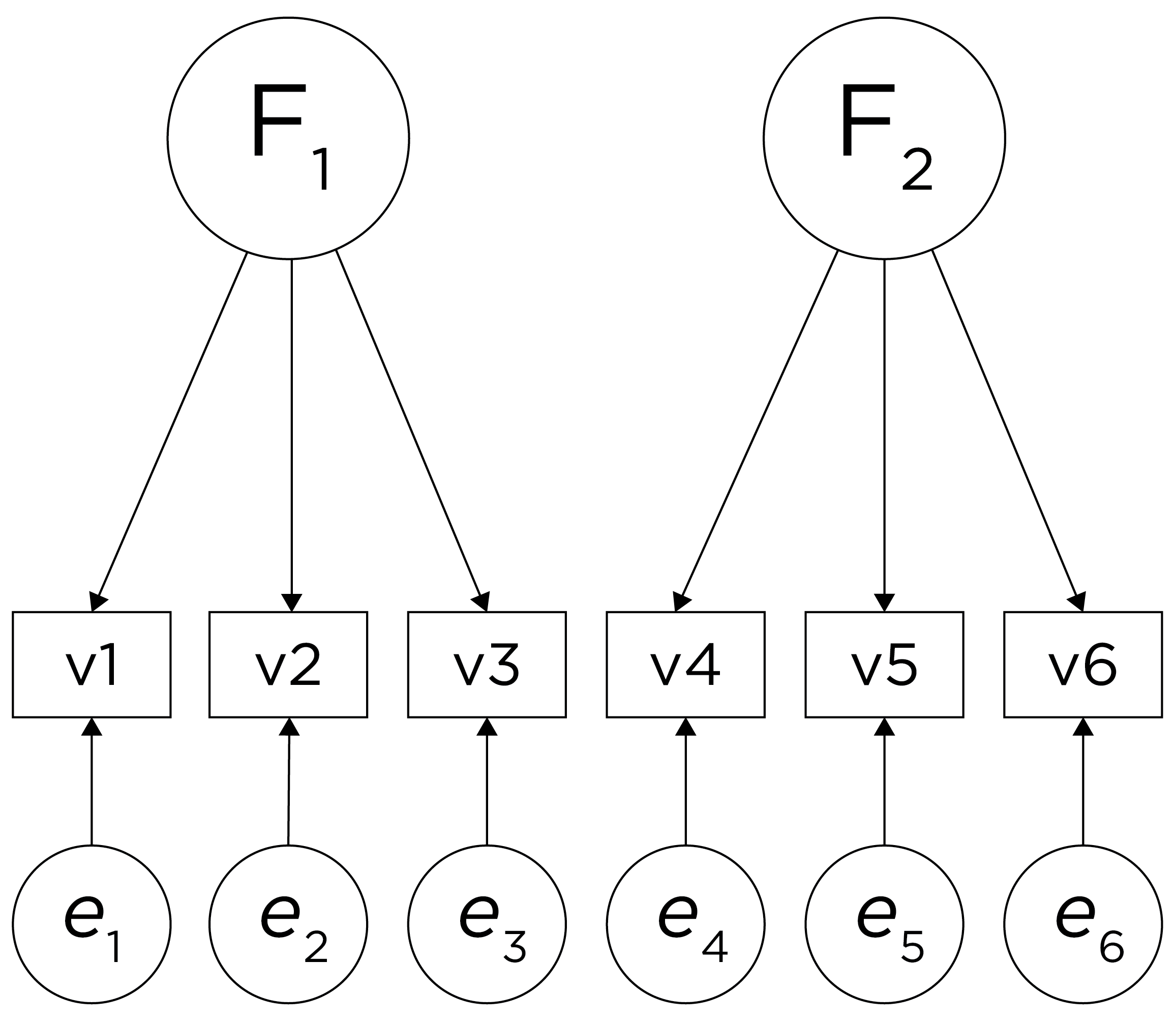
Figure 14.23: Example of a Factor Structure From an Orthogonal Rotation.
Sometimes, however, the two factors and their constituent variables may be correlated. Examples of two correlated factors may be depression and anxiety. When the two factors are correlated in reality, if we make them uncorrelated, this would result in an inaccurate model. Oblique rotation allows for factors to be correlated and yields axes with an angle of less than 90 degrees. However, if the factors have low correlation (e.g., .2 or less), you can likely continue with orthogonal rotation. Nevertheless, just because an oblique rotation allows for correlated factors does not mean that the factors will be correlated, so oblique rotation provides greater flexibility than orthogonal rotation. An example of a factor structure from an oblique rotation is in Figure 14.24. Results from an oblique rotation are more complicated than orthogonal rotation—they provide lots of output and are more complicated to interpret. In addition, oblique rotation might not yield a smooth answer if you have a relatively small sample size.
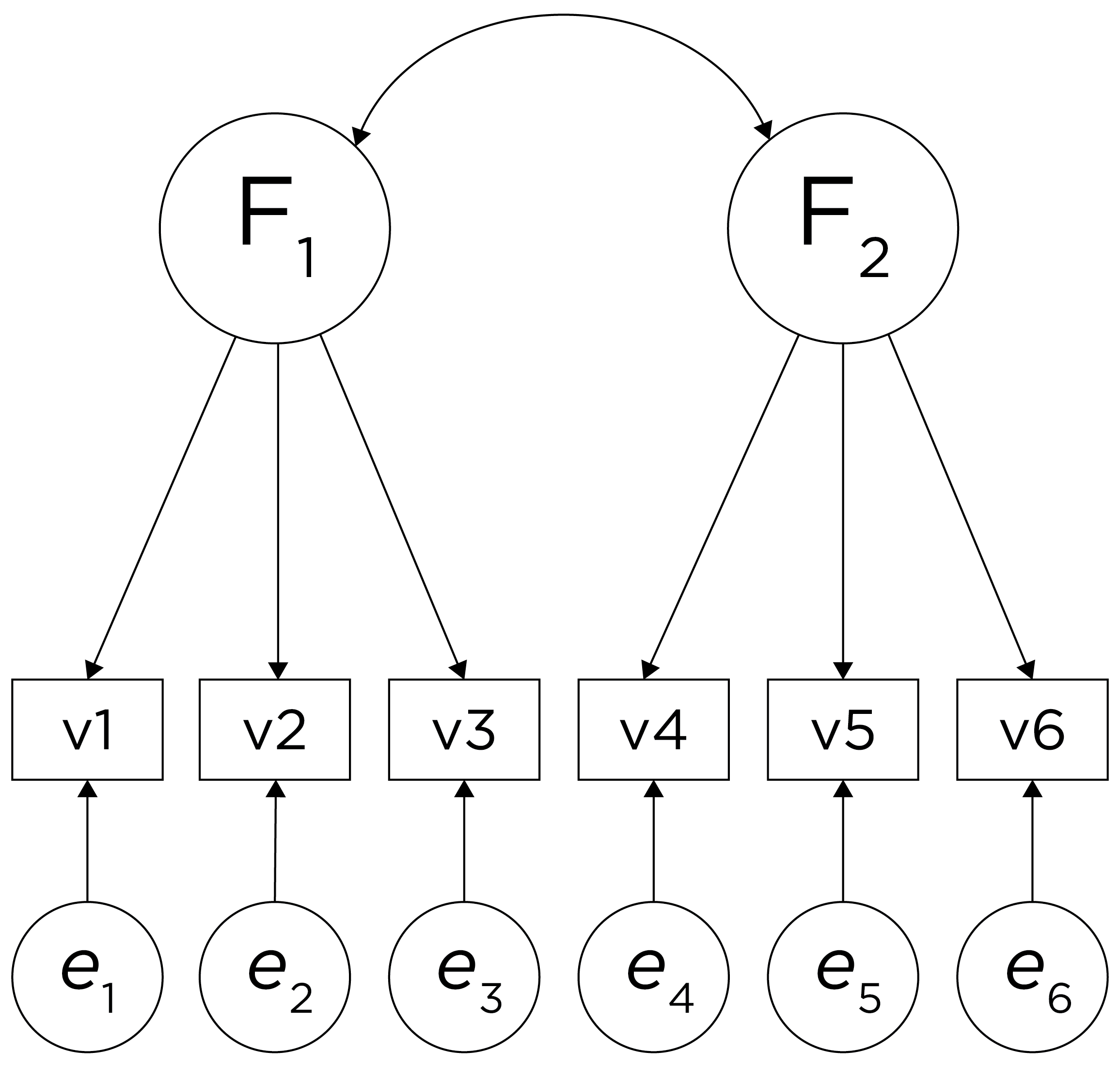
Figure 14.24: Example of a Factor Structure From an Oblique Rotation.
As an example of rotation based on interpretability, consider the Five-Factor Model of Personality (the Big Five), which goes by the acronym, OCEAN: Openness, Conscientiousness, Extraversion, Agreeableness, and Neuroticism. Although the five factors of personality are somewhat correlated, we can use rotation to ensure they are maximally independent. Upon rotation, extraversion and neuroticism are essentially uncorrelated, as depicted in Figure 14.25. The other pole of extraversion is intraversion and the other pole of neuroticism might be emotional stability or calmness.
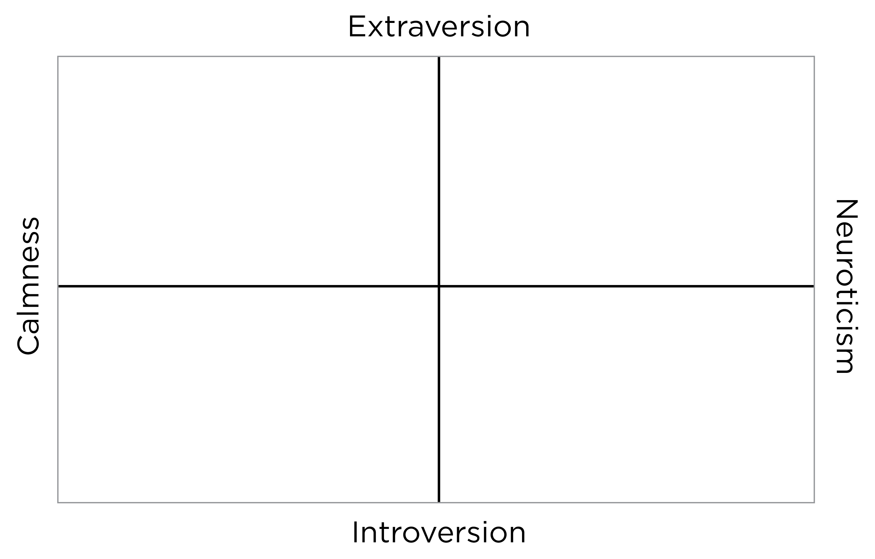
Figure 14.25: Example of a Factor Rotation of Neuroticism and Extraversion.
Simple structure is achieved when each variable loads highly onto as few factors as possible (i.e., each item has only one significant or primary loading). Oftentimes this is not the case, so we choose our rotation method in order to decide if the factors can be correlated (an oblique rotation) or if the factors will be uncorrelated (an orthogonal rotation). If the factors are not correlated with each other, use an orthogonal rotation. The correlation between an item and a factor is a factor loading, which is simply a way to ask how much a variable is correlated with the underlying factor. However, its interpretation is more complicated if there are correlated factors!
An orthogonal rotation (e.g., varimax) can help with simplicity of interpretation because it seeks to yield simple structure without cross-loadings. Cross-loadings are instances where a variable loads onto multiple factors. My recommendation would always be to use an orthogonal rotation if you have reason to believe that finding simple structure in your data is possible; otherwise, the factors are extremely difficult to interpret—what exactly does a cross-loading even mean? However, you should always try an oblique rotation, too, to see how strongly the factors are correlated. If the factors are not correlated, an oblique rotation will resolve to yield similar results as an orthogonal rotation (and thus may be preferred over othogonal rotation given its flexibility). Examples of oblique rotations include oblimin and promax.
14.1.4.6 6. Model Selection and Interpretation
The next step of factor analysis is selecting and interpreting the model. One data matrix can lead to many different (correct) models—you must choose one based on the factor structure and theory. Use theory to interpret the model and label the factors. When interpreting others’ findings, do not rely just on the factor labels—look at the actual items to determine what they assess. What they are called matters much less than what the actual items are! This calls to mind the jingle-jangle fallacy. The jingle fallacy is the erroneous assumption that two different things are the same because they have the same label; the jangle fallacy is the erroneous assumption that two identical or near-identical things are different because they have different labels. Thus, it is important to evaluate the measures and what they actually assess, and not just to rely on labels and what they intend to assess.
14.1.5 The Downfall of Factor Analysis
The downfall of factor analysis is cross-validation. Cross-validating a factor structure would mean getting the same factor structure with a new sample. We want factor structures to show good replicability across samples. However, cross-validation often falls apart. The way to attempt to replicate a factor structure in an independent sample is to use CFA to set everything up and test the hypothesized factor structure in the independent sample.
14.1.6 What to Do with Factors
What can you do with factors once you have them? In SEM, factors have meaning. You can use them as predictors, mediators, moderators, or outcomes. And, using latent factors in SEM helps disattenuate associations for measurement error, as described in Section 5.6.3. People often want to use factors outside of SEM, but there is confusion here: When researchers find that three variables load onto Factor A, the researchers often combine those three using a sum or average—but this is not accurate. If you just add or average them, this ignores the factor loadings and the error. A mean or sum score is a measurement model that assumes that all items have the same factor loading (i.e., a loading of 1) and no error (residual of 0), which is unrealistic. Another solution is to form a linear composite by adding and weighting the variables by the factor loadings, which retains the differences in correlations (i.e., a weighted sum), but this still ignores the estimated error, so it still may not be generalizable and meaningful. At the same time, weighted sums may be less generalizable than unit-weighted composites where each variable is given equal weight (Garb & Wood, 2019; Wainer, 1976) because some variability in factor loadings likely reflects sampling error.
A comparison of various measurement models is in Table 14.1.
| Measurement Model | Items’ Factor Loadings | Items’ Residuals/Error |
|---|---|---|
| Mean/Sum Score | All are the same (fixed to 1) | Assumes items are measured without error (fixed to 0) |
| PCA or Weighted Mean/Sum Score | Allowed to differ | Assumes items are measured without error (fixed to 0) |
| Latent Variable Modeling (CFA, EFA, SEM, IRT) | Allowed to differ | Estimates error for each item |
14.1.7 Missing Data Handling
The PCA default in SPSS is listwise deletion of missing data: if a participant is missing data on any variable, the subject gets excluded from the analysis, so you might end up with too few participants.
Instead, use a correlation matrix with pairwise deletion for PCA with missing data.
Maximum likelihood factor analysis can make use of all available data points for a participant, even if they are missing some data points.
Mplus, which is often used for SEM and factor analysis, will notify you if you are removing many participants in CFA/EFA.
The lavaan package (Rosseel et al., 2022) in R also notifies you if you are removing participants in CFA/SEM models.
14.1.8 Troubleshooting Improper Solutions
A PCA will always converge; however, a factor analysis model may not converge. If a factor analysis model does not converge, you will need to modify the model to get it to converge. Model identification is described here.
In addition, a factor analysis model may converge but be improper. For example, if the factor analysis model has a negative residual variance or correlation above 1, the model is improper. A negative residual variance is also called a Heywood case. Problematic parameters such as a negative residual variance or correlation above 1 can lead to problems with other parameters in the model. It is thus preferable to avoid or address improper solutions. A negative residual variance or correlation above 1 could be caused by a variety of things such as a misspecified model, too many factors, too few indicators per factor, or too few participants (relative to the complexity of the model). Another issue that could arise is a non-positive definite matrix. A non-positive definite matrix could also be caused by a variety of things such as multicollinearity or singularity, variables with zero variance, too many variables relative to the sample size, or too many factors.
Here are various ways you may troubleshoot improper solutions in factor analysis:
- Modify the model to be a represent a truer representation of the data-generating process
- Simplify the model
- Estimate fewer paths/parameters
- Reduce the number of factors estimated/extracted
- Reduce the number of variables included
- Increase the sample size
- Increase the number of indicators per factor
- Examine the data for outliers
- Drop the offending item that has a negative residual variance (if theoretically justifiable because the item may be poorly performing)
- Use different starting values
- Test whether the negative residual variance is significantly different from zero; if not, can consider fixing it to zero (though this is not an ideal solution)
- Examine the data for possible outliers
- Use regularization with constraints so the residual variances do not become negative
14.2 Getting Started
14.2.1 Load Libraries
Code
library("petersenlab") #to install: install.packages("remotes"); remotes::install_github("DevPsyLab/petersenlab")
library("lavaan")
library("psych")
library("corrplot")
library("nFactors")
library("semPlot")
library("lavaan")
library("semTools")
library("dagitty")
library("BifactorIndicesCalculator") #to install: install.packages("remotes"); remotes::install_github("ddueber/BifactorIndicesCalculator")
library("kableExtra")
library("MOTE")
library("tidyverse")
library("here")
library("tinytex")
library("knitr")
library("rmarkdown")14.2.3 Prepare Data
14.2.3.1 Add Missing Data
Adding missing data to dataframes helps make examples more realistic to real-life data and helps you get in the habit of programming to account for missing data. For reproducibility, I set the seed below. Using the same seed will yield the same answer every time. There is nothing special about this particular seed.
HolzingerSwineford1939 is a data set from the lavaan package (Rosseel et al., 2022) that contains mental ability test scores (x1–x9) for seventh- and eighth-grade children.
Code
set.seed(52242)

varNames <- names(HolzingerSwineford1939)
dimensionsDf <- dim(HolzingerSwineford1939)
unlistedDf <- unlist(HolzingerSwineford1939)
unlistedDf[sample(
  1:length(unlistedDf),
  size = .15 * length(unlistedDf))] <- NA
HolzingerSwineford1939 <- as.data.frame(matrix(
  unlistedDf,
  ncol = dimensionsDf[2]))
names(HolzingerSwineford1939) <- varNames
vars <- c("x1","x2","x3","x4","x5","x6","x7","x8","x9")
14.3 Descriptive Statistics and Correlations
Before conducting a factor analysis, it is important examine descriptive statistics and correlations among variables.
14.3.1 Descriptive Statistics
Descriptive statistics are presented in Table ??.
Code
summaryTable <- HolzingerSwineford1939 %>%
  dplyr::select(all_of(vars)) %>%
  summarise(across(
    everything(),
    .fns = list(
      n = ~ length(na.omit(.)),
      missingness = ~ mean(is.na(.)) * 100,
      M = ~ mean(., na.rm = TRUE),
      SD = ~ sd(., na.rm = TRUE),
      min = ~ min(., na.rm = TRUE),
      max = ~ max(., na.rm = TRUE),
      skewness = ~ psych::skew(., na.rm = TRUE),
      kurtosis = ~ kurtosi(., na.rm = TRUE)),
    .names = "{.col}.{.fn}")) %>%
  pivot_longer(
    cols = everything(),
    names_to = c("variable","index"),
    names_sep = "\\.") %>%
  pivot_wider(
    names_from = index,
    values_from = value)

summaryTableTransposed <- summaryTable[-1] %>%
  t() %>%
  as.data.frame() %>%
  setNames(summaryTable$variable) %>%
  round(., digits = 2)

summaryTableTransposed
14.3.2 Correlations
           x1          x2        x3        x4        x5        x6          x7
x1 1.00000000  0.31671519 0.4592132 0.4009470 0.3060026 0.3204367  0.04336147
x2 0.31671519  1.00000000 0.3373084 0.1474393 0.1925946 0.1686010 -0.08744963
x3 0.45921315  0.33730843 1.0000000 0.1770624 0.1504923 0.1930589  0.08771510
x4 0.40094704  0.14743932 0.1770624 1.0000000 0.7314651 0.6796334  0.14825470
x5 0.30600259  0.19259455 0.1504923 0.7314651 1.0000000 0.6931306  0.10592715
x6 0.32043667  0.16860100 0.1930589 0.6796334 0.6931306 1.0000000  0.09881660
x7 0.04336147 -0.08744963 0.0877151 0.1482547 0.1059272 0.0988166  1.00000000
x8 0.25775028  0.09357234 0.2012953 0.1297963 0.2134497 0.1856636  0.48743045
x9 0.34289304  0.20083617 0.3959389 0.1917355 0.2605835 0.1805793  0.34622036
           x8        x9
x1 0.25775028 0.3428930
x2 0.09357234 0.2008362
x3 0.20129535 0.3959389
x4 0.12979634 0.1917355
x5 0.21344970 0.2605835
x6 0.18566357 0.1805793
x7 0.48743045 0.3462204
x8 1.00000000 0.4637719
x9 0.46377193 1.0000000
Correlation matrices of various types using the cor.table() function from the petersenlab package (Petersen, 2025) are in Tables 14.2, 14.3, and 14.4.
Code
| x1 | x2 | x3 | x4 | x5 | x6 | x7 | x8 | x9 | |
|---|---|---|---|---|---|---|---|---|---|
| 1. x1.r | 1.00 | .32*** | .46*** | .40*** | .31*** | .32*** | .04 | .26*** | .34*** |
| 2. sig | NA | .00 | .00 | .00 | .00 | .00 | .52 | .00 | .00 |
| 3. n | 251 | 221 | 211 | 208 | 215 | 205 | 221 | 219 | 215 |
| 4. x2.r | .32*** | 1.00 | .34*** | .15* | .19*** | .17* | -.09 | .09 | .20*** |
| 5. sig | .00 | NA | .00 | .03 | .00 | .01 | .18 | .16 | .00 |
| 6. n | 221 | 265 | 225 | 227 | 228 | 216 | 234 | 227 | 229 |
| 7. x3.r | .46*** | .34*** | 1.00 | .18* | .15* | .19* | .09 | .20*** | .40*** |
| 8. sig | .00 | .00 | NA | .01 | .03 | .01 | .19 | .00 | .00 |
| 9. n | 211 | 225 | 255 | 211 | 215 | 206 | 227 | 219 | 220 |
| 10. x4.r | .40*** | .15* | .18* | 1.00 | .73*** | .68*** | .15* | .13† | .19*** |
| 11. sig | .00 | .03 | .01 | NA | .00 | .00 | .03 | .06 | .00 |
| 12. n | 208 | 227 | 211 | 252 | 216 | 209 | 224 | 217 | 215 |
| 13. x5.r | .31*** | .19*** | .15* | .73*** | 1.00 | .69*** | .11 | .21*** | .26*** |
| 14. sig | .00 | .00 | .03 | .00 | NA | .00 | .11 | .00 | .00 |
| 15. n | 215 | 228 | 215 | 216 | 259 | 217 | 226 | 222 | 219 |
| 16. x6.r | .32*** | .17* | .19* | .68*** | .69*** | 1.00 | .10 | .19* | .18* |
| 17. sig | .00 | .01 | .01 | .00 | .00 | NA | .15 | .01 | .01 |
| 18. n | 205 | 216 | 206 | 209 | 217 | 248 | 218 | 214 | 209 |
| 19. x7.r | .04 | -.09 | .09 | .15* | .11 | .10 | 1.00 | .49*** | .35*** |
| 20. sig | .52 | .18 | .19 | .03 | .11 | .15 | NA | .00 | .00 |
| 21. n | 221 | 234 | 227 | 224 | 226 | 218 | 266 | 231 | 226 |
| 22. x8.r | .26*** | .09 | .20*** | .13† | .21*** | .19* | .49*** | 1.00 | .46*** |
| 23. sig | .00 | .16 | .00 | .06 | .00 | .01 | .00 | NA | .00 |
| 24. n | 219 | 227 | 219 | 217 | 222 | 214 | 231 | 259 | 222 |
| 25. x9.r | .34*** | .20*** | .40*** | .19*** | .26*** | .18* | .35*** | .46*** | 1.00 |
| 26. sig | .00 | .00 | .00 | .00 | .00 | .01 | .00 | .00 | NA |
| 27. n | 215 | 229 | 220 | 215 | 219 | 209 | 226 | 222 | 257 |
| x1 | x2 | x3 | x4 | x5 | x6 | x7 | x8 | x9 | |
|---|---|---|---|---|---|---|---|---|---|
| 1. x1 | 1.00 | ||||||||
| 2. x2 | .32*** | 1.00 | |||||||
| 3. x3 | .46*** | .34*** | 1.00 | ||||||
| 4. x4 | .40*** | .15* | .18* | 1.00 | |||||
| 5. x5 | .31*** | .19*** | .15* | .73*** | 1.00 | ||||
| 6. x6 | .32*** | .17* | .19* | .68*** | .69*** | 1.00 | |||
| 7. x7 | .04 | -.09 | .09 | .15* | .11 | .10 | 1.00 | ||
| 8. x8 | .26*** | .09 | .20*** | .13† | .21*** | .19* | .49*** | 1.00 | |
| 9. x9 | .34*** | .20*** | .40*** | .19*** | .26*** | .18* | .35*** | .46*** | 1.00 |
| x1 | x2 | x3 | x4 | x5 | x6 | x7 | x8 | x9 | |
|---|---|---|---|---|---|---|---|---|---|
| 1. x1 | 1.00 | ||||||||
| 2. x2 | .32 | 1.00 | |||||||
| 3. x3 | .46 | .34 | 1.00 | ||||||
| 4. x4 | .40 | .15 | .18 | 1.00 | |||||
| 5. x5 | .31 | .19 | .15 | .73 | 1.00 | ||||
| 6. x6 | .32 | .17 | .19 | .68 | .69 | 1.00 | |||
| 7. x7 | .04 | -.09 | .09 | .15 | .11 | .10 | 1.00 | ||
| 8. x8 | .26 | .09 | .20 | .13 | .21 | .19 | .49 | 1.00 | |
| 9. x9 | .34 | .20 | .40 | .19 | .26 | .18 | .35 | .46 | 1.00 |
Pairs panel plots were generated using the psych package (Revelle, 2022).
Correlation plots were generated using the corrplot package (Wei & Simko, 2021).
A pairs panel plot is in Figure 14.26.
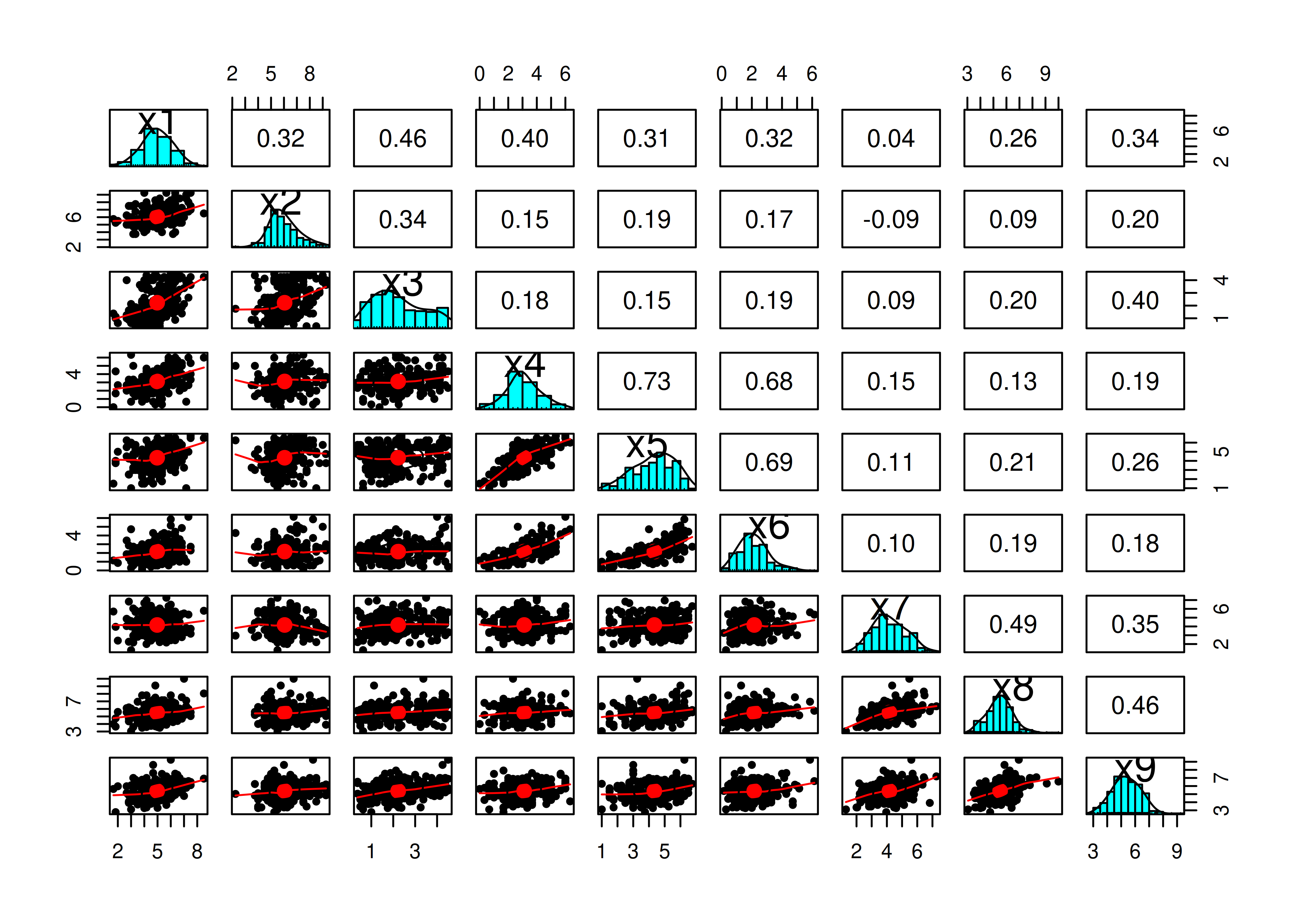
Figure 14.26: Pairs Panel Plot.
A correlation plot is in Figure 14.27.
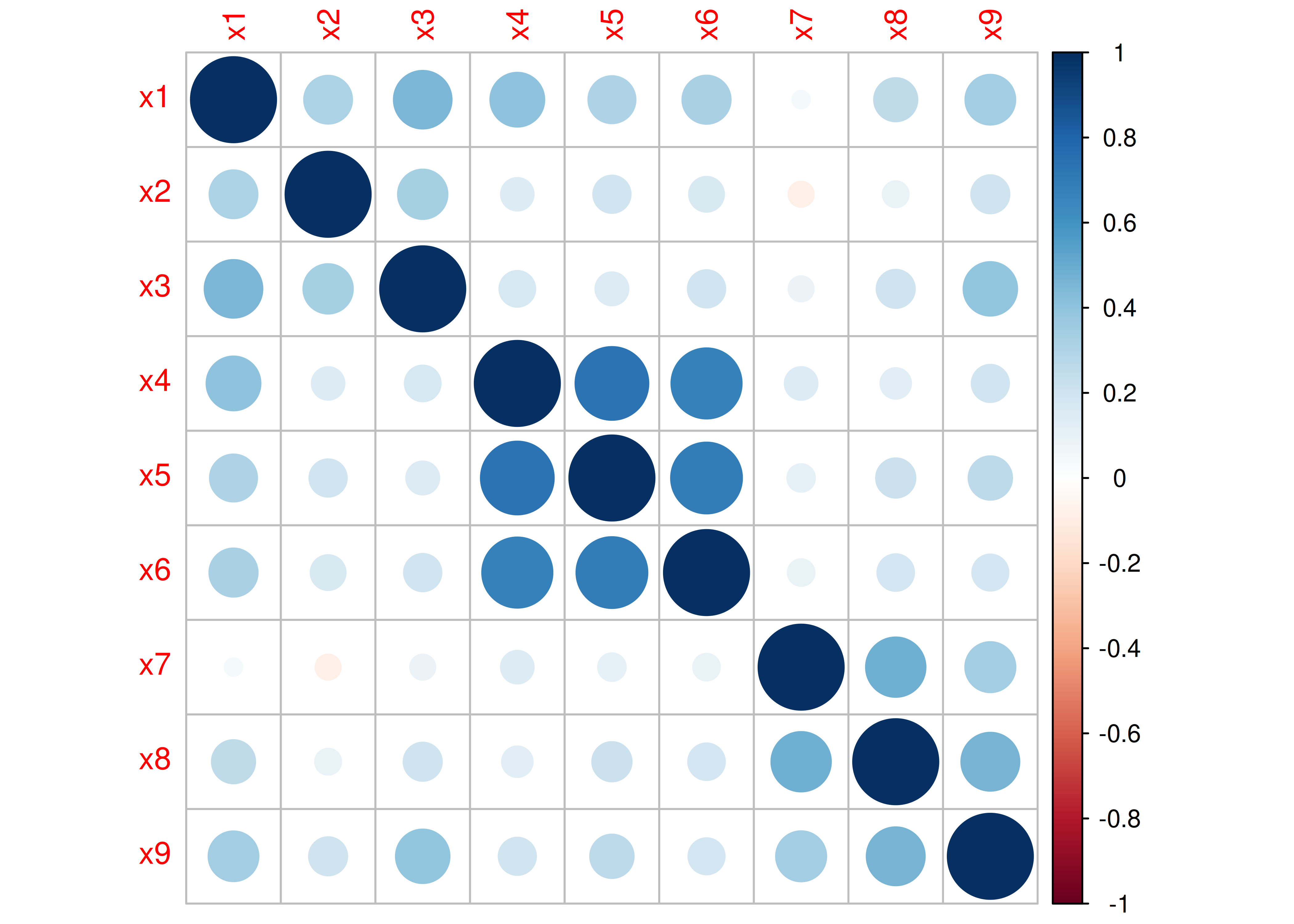
Figure 14.27: Correlation Plot.
14.3.3 Kaiser-Meyer-Oklin (KMO) Test
The Kaiser-Meyer-Oklin (KMO) measure of sampling adequacy (Kaiser, 1970; Kaiser & Rice, 1974) evaluates the extent to which a set of variables is suitable for factor analysis. It indicates the proportion of variance in your variables that might be caused by underlying factors, where a higher proportion indicates the data are potentially more suitable for factor analysis. The following criteria are used for evaluating KMO (Kaiser, 1974):
- Above 0.90 - Marvelous
- 0.80 to 0.90 - Meritorious
- 0.7 to 0.80 - Average
- 0.60 to 0.70 - Mediocre
- 0.50 to 0.60 - Terrible
- Below 0.50 - Unacceptable
Kaiser-Meyer-Olkin factor adequacy
Call: psych::KMO(r = HolzingerSwineford1939[, vars])
Overall MSA =  0.74
MSA for each item =
  x1   x2   x3   x4   x5   x6   x7   x8   x9
0.77 0.78 0.74 0.72 0.74 0.82 0.58 0.68 0.78
14.3.4 Determinant of a Correlation Matrix
The determinant of a correlation matrix can be used to evaluate the potential for multicollinearity, which can be problematic in factor analysis. For purposes of pursuing factor analysis, the determinant of the correlation matrix should be greater than 0.00001 (Field et al., 2012).
Code
[1] 0.0471407214.3.5 Bartlett’s Test of Sphericity
Bartlett’s test of sphericity evaluates whether the correlations between the variables are significantly different from zero. A significant Bartlett’s test indicates that the correlations between the variables significantly differ from zero and that factor analysis may be able to be used.
$chisq
[1] 290.6978

$p.value
[1] 1.378106e-41

$df
[1] 36
14.4 Factor Analysis
14.4.1 Exploratory Factor Analysis (EFA)
I introduced exploratory factor analysis (EFA) models in Section 14.1.4.3.1.
14.4.1.1 Determine number of factors
Determine the number of factors to retain using the Scree plot and Very Simple Structure plot.
14.4.1.1.1 Scree Plot
Scree plots were generated using the psych (Revelle, 2022) and nFactors (Raiche & Magis, 2020) packages.
The optimal coordinates and the acceleration factor attempt to operationalize the Cattell scree test: i.e., the “elbow” of the scree plot (Ruscio & Roche, 2012).
The optimal coordinators factor is quantified using a series of linear equations to determine whether observed eigenvalues exceed the predicted values.
The acceleration factor is quantified using the acceleration of the curve, that is, the second derivative.
The Kaiser-Guttman rule states to keep principal components whose eigenvalues are greater than 1.
However, for exploratory factor analysis (as opposed to PCA), the criterion is to keep the factors whose eigenvalues are greater than zero (i.e., not the factors whose eigenvalues are greater than 1) (Dinno, 2014).
The number of factors to keep would depend on which criteria one uses. Based on the rule to keep factors whose eigenvalues are greater than zero and based on the parallel test, we would keep three factors. However, based on the Cattell scree test (as operationalized by the optimal coordinates and acceleration factor), we would keep one factor. Therefore, interpretability of the factors would be important for deciding between whether to keep one, two, or three factors.
A scree plot from a parallel analysis is in Figure 14.28.
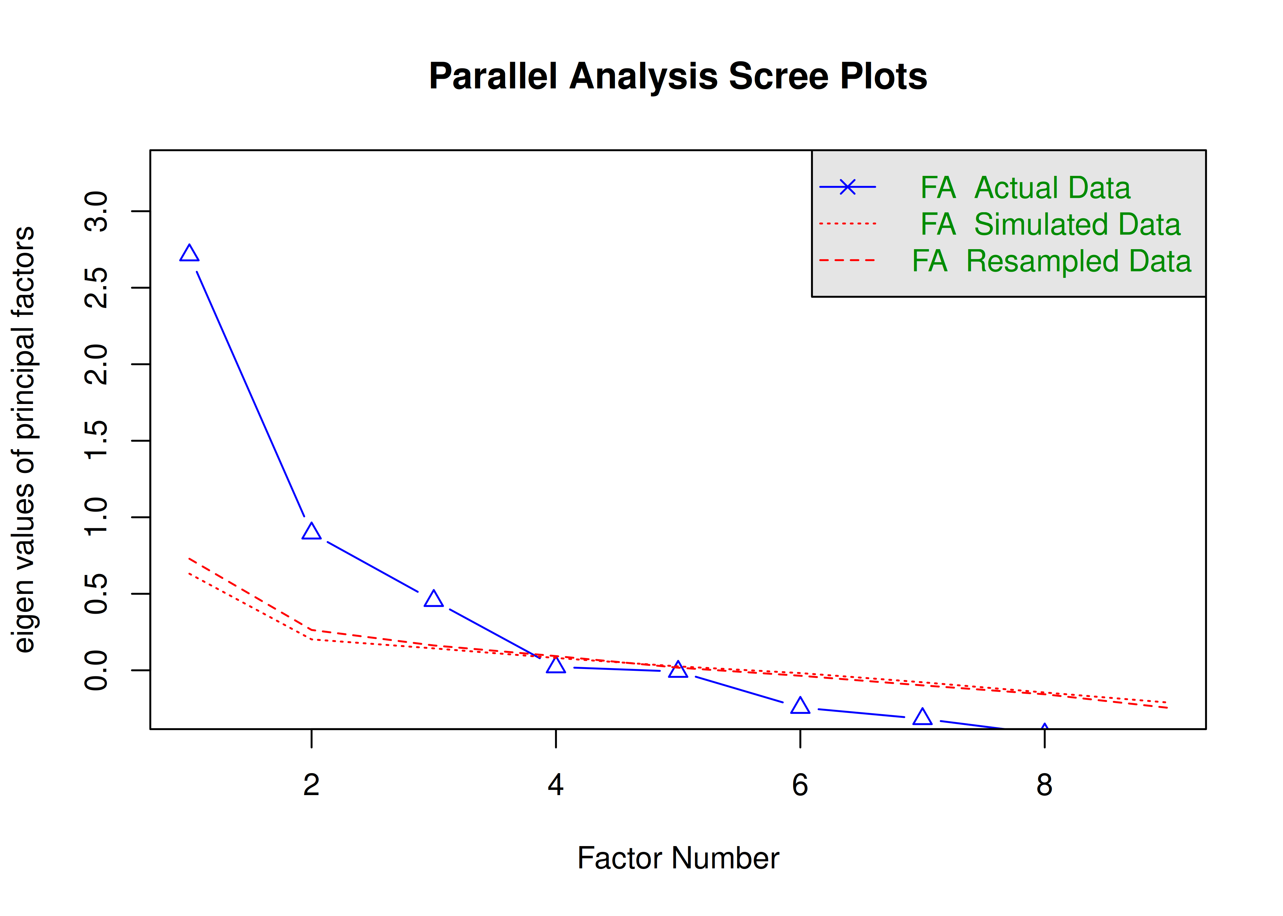
Figure 14.28: Scree Plot from Parallel Analysis in Exploratory Factor Analysis.
Parallel analysis suggests that the number of factors = 3 and the number of components = NA A scree plot from EFA is in Figure 14.29.
Code
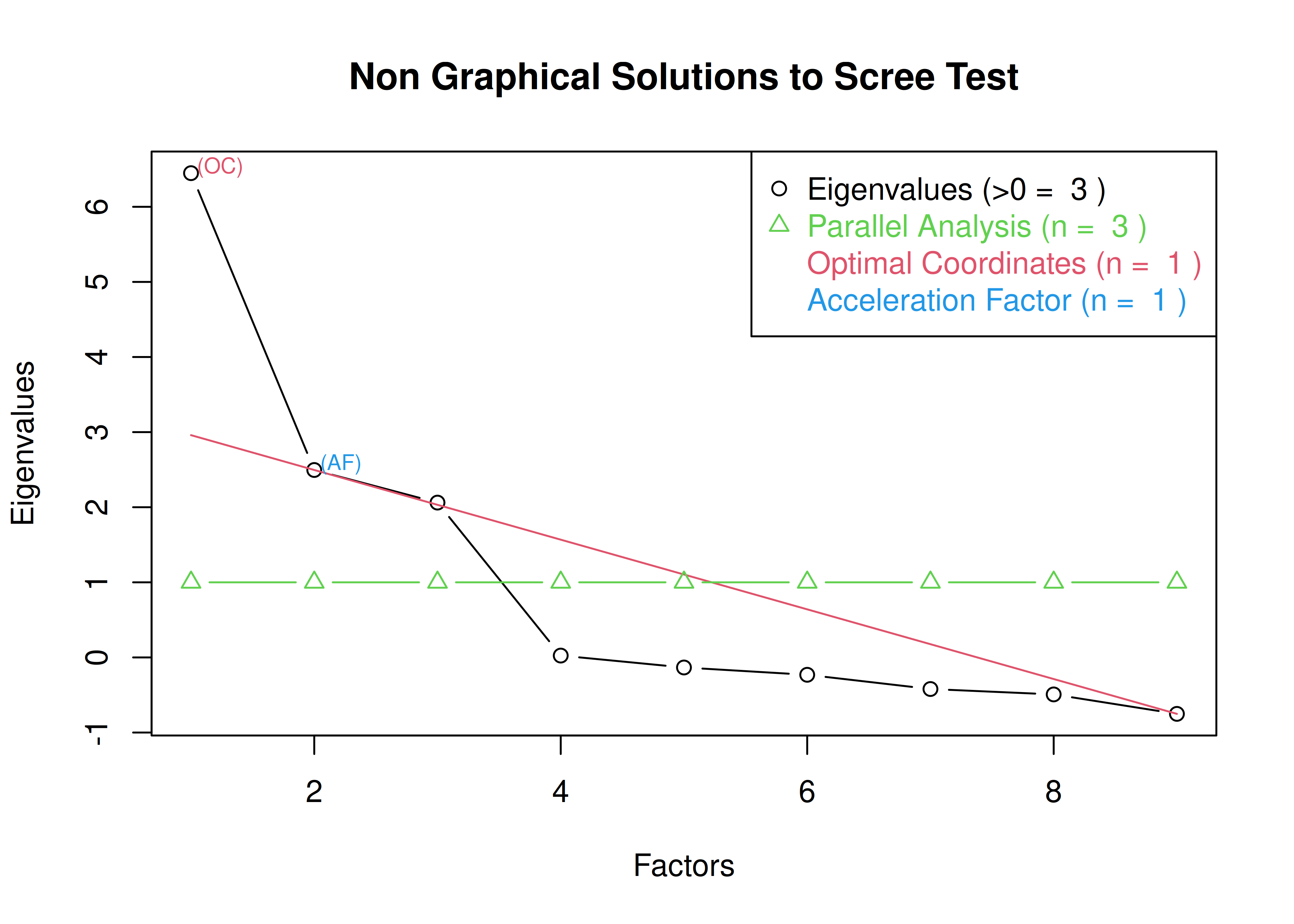
Figure 14.29: Scree Plot in Exploratory Factor Analysis.
14.4.1.1.2 Very Simple Structure (VSS) Plot
The very simple structure (VSS) is another criterion that can be used to determine the optimal number of factors or components to retain.
Using the VSS criterion, the optimal number of factors to retain is the number of factors that maximizes the VSS criterion (Revelle & Rocklin, 1979).
The VSS criterion is evaluated with models in which factor loadings for a given item that are less than the maximum factor loading for that item are suppressed to zero, thus forcing simple structure (i.e., no cross-loadings).
The goal is finding a factor structure with interpretability so that factors are clearly distinguishable.
Thus, we want to identify the number of factors with the highest VSS criterion (i.e., the highest line).
Very simple structure (VSS) plots were generated using the psych package (Revelle, 2022).
The output also provides additional criteria by which to determine the optimal number of factors, each for which lower values are better, including the Velicer minimum average partial (MAP) test, the Bayesian information criterion (BIC), the sample size-adjusted BIC (SABIC), and the root mean square error of approximation (RMSEA).
14.4.1.1.2.1 Orthogonal (Varimax) rotation
In the example with orthogonal rotation below, the VSS criterion is highest with 3 or 4 factors. A three-factor solution is supported by the lowest BIC, whereas a four-factor solution is supported by the lowest SABIC.
A VSS plot is in Figure 14.30.
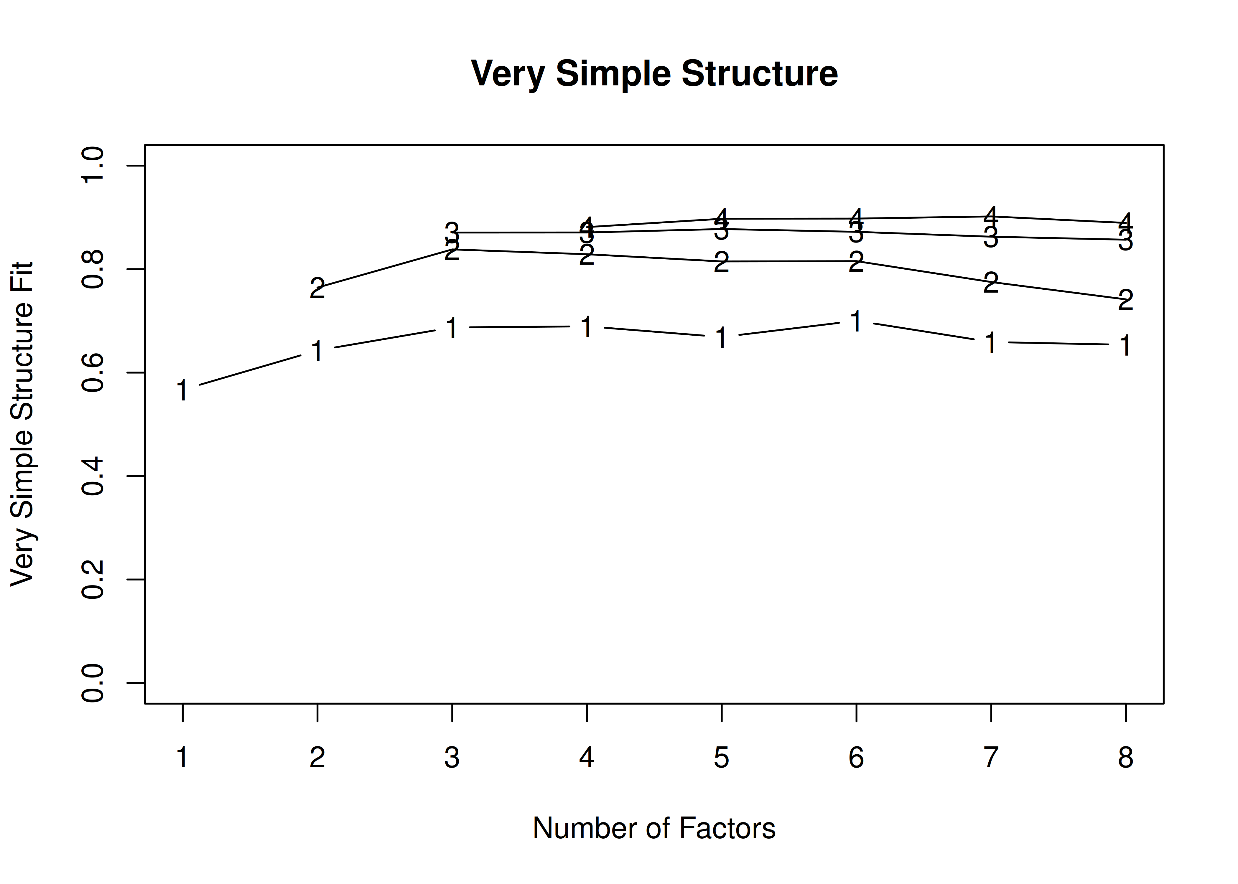
Figure 14.30: Very Simple Structure Plot With Orthogonal Rotation in Exploratory Factor Analysis.
Very Simple Structure
Call: vss(x = HolzingerSwineford1939[, vars], rotate = "varimax", fm = "ml")
VSS complexity 1 achieves a maximimum of 0.7  with  4  factors
VSS complexity 2 achieves a maximimum of 0.84  with  3  factors

The Velicer MAP achieves a minimum of 0.07  with  2  factors
BIC achieves a minimum of  -32.61  with  3  factors
Sample Size adjusted BIC achieves a minimum of  -5.65  with  4  factors

Statistics by number of factors
  vss1 vss2   map dof   chisq    prob sqresid  fit RMSEA   BIC  SABIC complex
1 0.57 0.00 0.078  27 3.2e+02 2.3e-52     7.1 0.57 0.191 168.4 254.05     1.0
2 0.64 0.76 0.067  19 1.4e+02 1.2e-20     3.9 0.76 0.146  32.5  92.75     1.2
3 0.69 0.84 0.071  12 3.6e+01 3.4e-04     2.1 0.87 0.081 -32.6   5.45     1.3
4 0.69 0.83 0.125   6 9.6e+00 1.4e-01     2.0 0.88 0.044 -24.7  -5.65     1.4
5 0.67 0.81 0.199   1 1.8e+00 1.8e-01     1.6 0.90 0.050  -3.9  -0.77     1.5
6 0.70 0.82 0.403  -3 2.6e-08      NA     1.6 0.91    NA    NA     NA     1.5
7 0.66 0.78 0.447  -6 0.0e+00      NA     1.4 0.91    NA    NA     NA     1.6
8 0.65 0.74 1.000  -8 0.0e+00      NA     1.3 0.92    NA    NA     NA     1.7
   eChisq    SRMR eCRMS  eBIC
1 5.5e+02 1.6e-01 0.184 396.3
2 1.6e+02 8.7e-02 0.119  53.8
3 1.2e+01 2.3e-02 0.040 -56.7
4 4.5e+00 1.4e-02 0.035 -29.7
5 8.0e-01 6.1e-03 0.036  -4.9
6 1.3e-08 7.7e-07    NA    NA
7 2.1e-13 3.1e-09    NA    NA
8 2.1e-16 1.0e-10    NA    NA
Multiple VSS-related fit indices are in Figure 14.31.
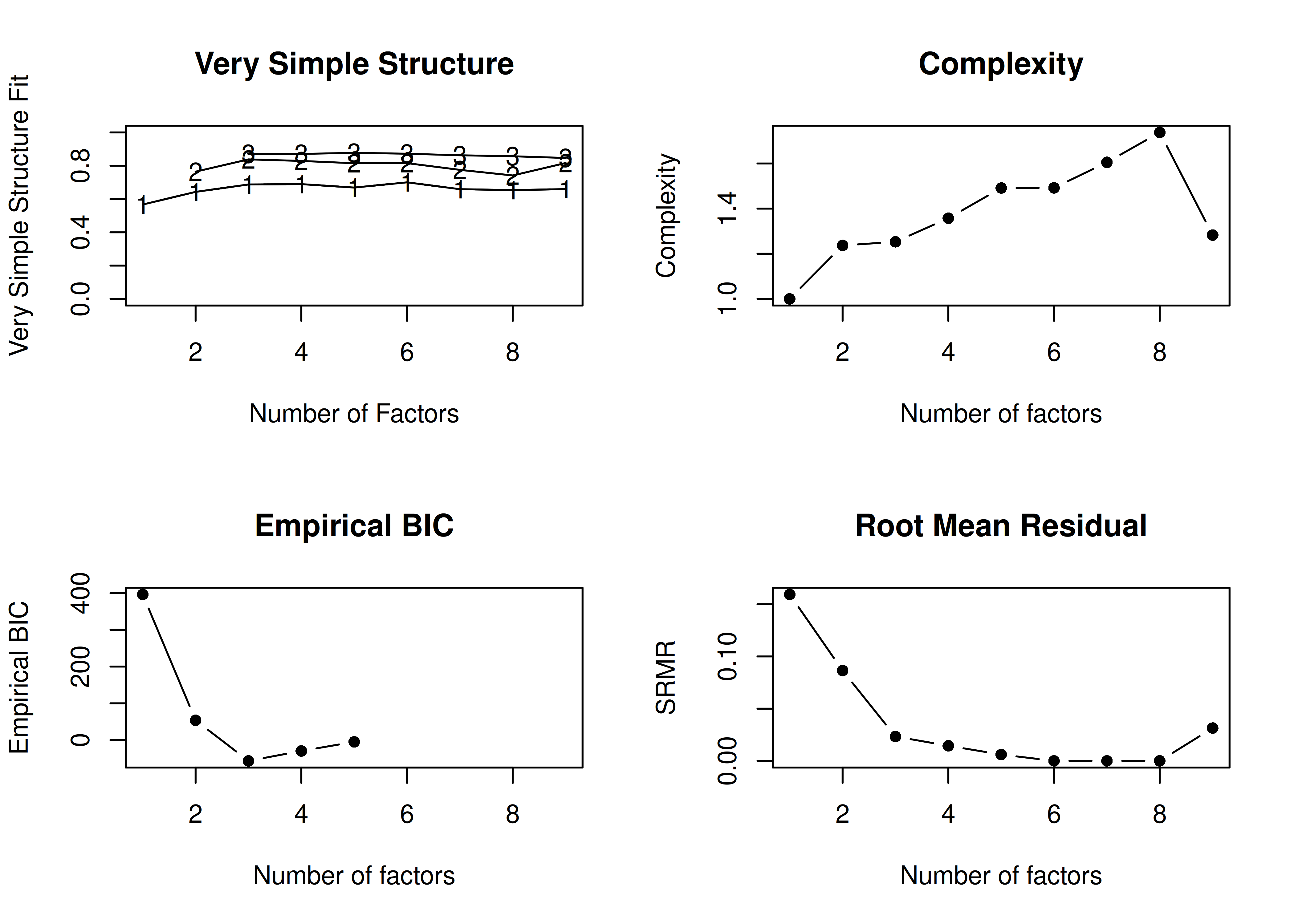
Figure 14.31: Very Simple Structure-Related Indices With Orthogonal Rotation in Exploratory Factor Analysis.
Number of factors
Call: vss(x = x, n = n, rotate = rotate, diagonal = diagonal, fm = fm,
    n.obs = n.obs, plot = FALSE, title = title, use = use, cor = cor)
VSS complexity 1 achieves a maximimum of Although the vss.max shows  6  factors, it is probably more reasonable to think about  4  factors
VSS complexity 2 achieves a maximimum of 0.84  with  3  factors
The Velicer MAP achieves a minimum of 0.07  with  2  factors
Empirical BIC achieves a minimum of  -56.69  with  3  factors
Sample Size adjusted BIC achieves a minimum of  -5.65  with  4  factors

Statistics by number of factors
  vss1 vss2   map dof   chisq    prob sqresid  fit RMSEA   BIC  SABIC complex
1 0.57 0.00 0.078  27 3.2e+02 2.3e-52     7.1 0.57 0.191 168.4 254.05     1.0
2 0.64 0.76 0.067  19 1.4e+02 1.2e-20     3.9 0.76 0.146  32.5  92.75     1.2
3 0.69 0.84 0.071  12 3.6e+01 3.4e-04     2.1 0.87 0.081 -32.6   5.45     1.3
4 0.69 0.83 0.125   6 9.6e+00 1.4e-01     2.0 0.88 0.044 -24.7  -5.65     1.4
5 0.67 0.81 0.199   1 1.8e+00 1.8e-01     1.6 0.90 0.050  -3.9  -0.77     1.5
6 0.70 0.82 0.403  -3 2.6e-08      NA     1.6 0.91    NA    NA     NA     1.5
7 0.66 0.78 0.447  -6 0.0e+00      NA     1.4 0.91    NA    NA     NA     1.6
8 0.65 0.74 1.000  -8 0.0e+00      NA     1.3 0.92    NA    NA     NA     1.7
9 0.66 0.82    NA  -9 4.4e+01      NA     2.5 0.85    NA    NA     NA     1.3
   eChisq    SRMR eCRMS  eBIC
1 5.5e+02 1.6e-01 0.184 396.3
2 1.6e+02 8.7e-02 0.119  53.8
3 1.2e+01 2.3e-02 0.040 -56.7
4 4.5e+00 1.4e-02 0.035 -29.7
5 8.0e-01 6.1e-03 0.036  -4.9
6 1.3e-08 7.7e-07    NA    NA
7 2.1e-13 3.1e-09    NA    NA
8 2.1e-16 1.0e-10    NA    NA
9 2.1e+01 3.1e-02    NA    NA
14.4.1.1.2.2 Oblique (Oblimin) rotation
In the example with oblique rotation below, the VSS criterion is highest with 3 factors. A three-factor solution is supported by the lowest BIC.
A VSS plot is in Figure 14.32.
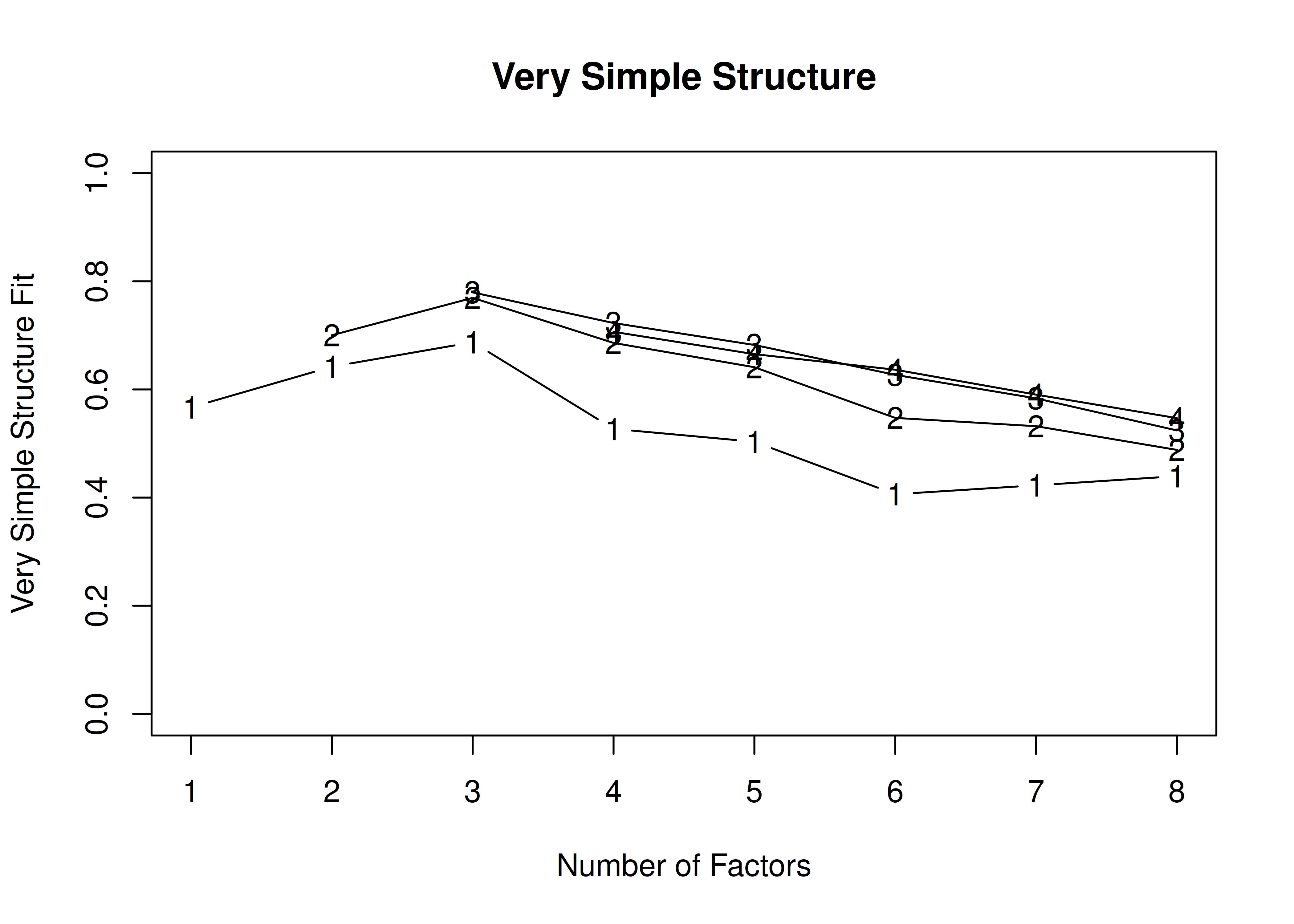
Figure 14.32: Very Simple Structure Plot With Oblique Rotation in Exploratory Factor Analysis.
Very Simple Structure
Call: vss(x = HolzingerSwineford1939[, vars], rotate = "oblimin", fm = "ml")
VSS complexity 1 achieves a maximimum of 0.69  with  3  factors
VSS complexity 2 achieves a maximimum of 0.77  with  3  factors

The Velicer MAP achieves a minimum of 0.07  with  2  factors
BIC achieves a minimum of  -32.61  with  3  factors
Sample Size adjusted BIC achieves a minimum of  -5.65  with  4  factors

Statistics by number of factors
  vss1 vss2   map dof   chisq    prob sqresid  fit RMSEA   BIC  SABIC complex
1 0.57 0.00 0.078  27 3.2e+02 2.3e-52     7.1 0.57 0.191 168.4 254.05     1.0
2 0.64 0.70 0.067  19 1.4e+02 1.2e-20     4.9 0.70 0.146  32.5  92.75     1.2
3 0.69 0.77 0.071  12 3.6e+01 3.4e-04     3.6 0.78 0.081 -32.6   5.45     1.2
4 0.53 0.69 0.125   6 9.6e+00 1.4e-01     4.8 0.71 0.044 -24.7  -5.65     1.4
5 0.50 0.64 0.199   1 1.8e+00 1.8e-01     5.3 0.68 0.050  -3.9  -0.77     1.5
6 0.41 0.55 0.403  -3 2.6e-08      NA     6.1 0.63    NA    NA     NA     1.8
7 0.42 0.53 0.447  -6 0.0e+00      NA     6.8 0.59    NA    NA     NA     1.5
8 0.44 0.49 1.000  -8 0.0e+00      NA     7.5 0.55    NA    NA     NA     1.5
   eChisq    SRMR eCRMS  eBIC
1 5.5e+02 1.6e-01 0.184 396.3
2 1.6e+02 8.7e-02 0.119  53.8
3 1.2e+01 2.3e-02 0.040 -56.7
4 4.5e+00 1.4e-02 0.035 -29.7
5 8.0e-01 6.1e-03 0.036  -4.9
6 1.3e-08 7.7e-07    NA    NA
7 2.1e-13 3.1e-09    NA    NA
8 2.1e-16 1.0e-10    NA    NA
Multiple VSS-related fit indices are in Figure 14.33.
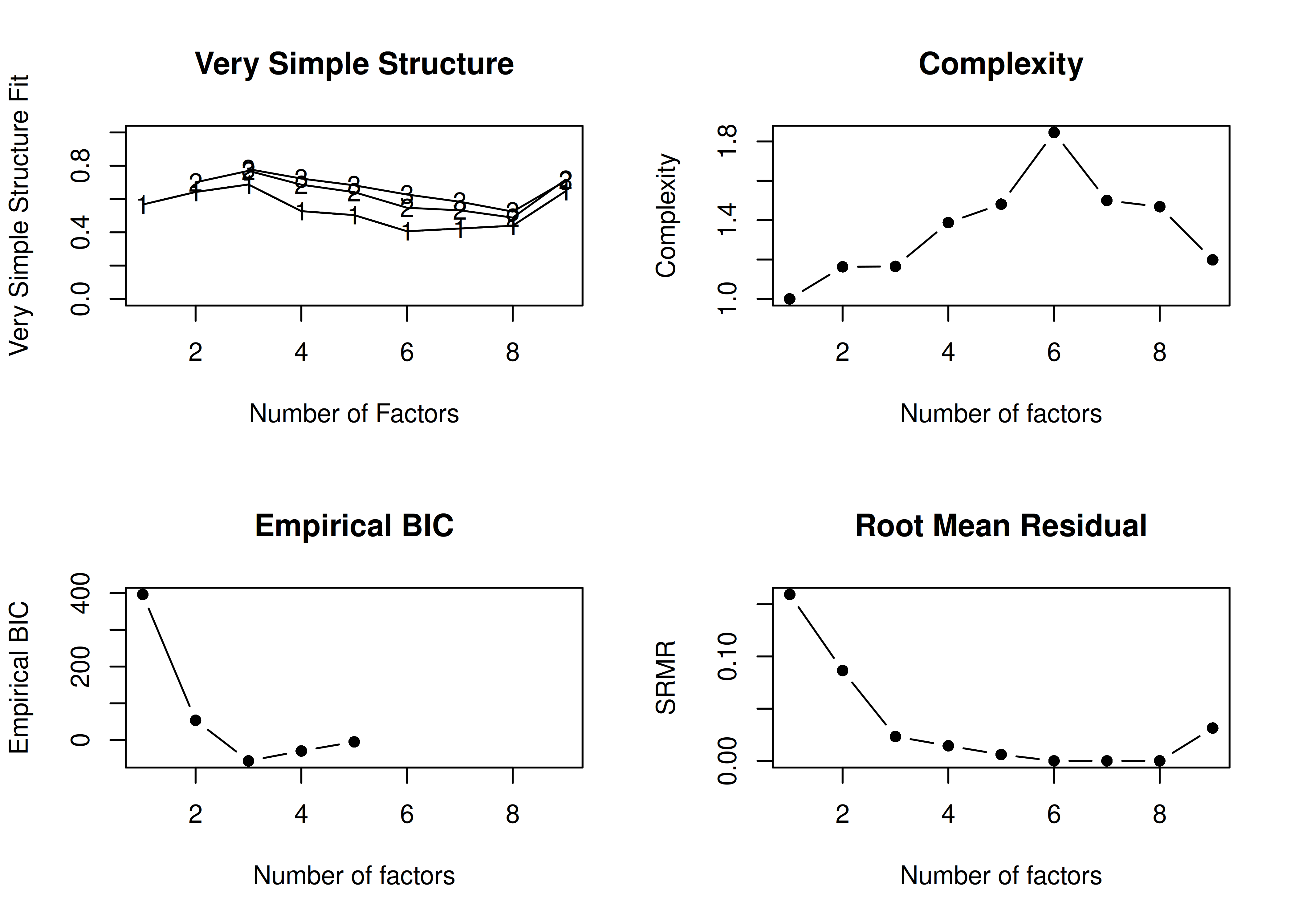
Figure 14.33: Very Simple Structure-Related Indices With Oblique Rotation in Exploratory Factor Analysis.
Number of factors
Call: vss(x = x, n = n, rotate = rotate, diagonal = diagonal, fm = fm,
    n.obs = n.obs, plot = FALSE, title = title, use = use, cor = cor)
VSS complexity 1 achieves a maximimum of 0.69  with  3  factors
VSS complexity 2 achieves a maximimum of 0.77  with  3  factors
The Velicer MAP achieves a minimum of 0.07  with  2  factors
Empirical BIC achieves a minimum of  -56.69  with  3  factors
Sample Size adjusted BIC achieves a minimum of  -5.65  with  4  factors

Statistics by number of factors
  vss1 vss2   map dof   chisq    prob sqresid  fit RMSEA   BIC  SABIC complex
1 0.57 0.00 0.078  27 3.2e+02 2.3e-52     7.1 0.57 0.191 168.4 254.05     1.0
2 0.64 0.70 0.067  19 1.4e+02 1.2e-20     4.9 0.70 0.146  32.5  92.75     1.2
3 0.69 0.77 0.071  12 3.6e+01 3.4e-04     3.6 0.78 0.081 -32.6   5.45     1.2
4 0.53 0.69 0.125   6 9.6e+00 1.4e-01     4.8 0.71 0.044 -24.7  -5.65     1.4
5 0.50 0.64 0.199   1 1.8e+00 1.8e-01     5.3 0.68 0.050  -3.9  -0.77     1.5
6 0.41 0.55 0.403  -3 2.6e-08      NA     6.1 0.63    NA    NA     NA     1.8
7 0.42 0.53 0.447  -6 0.0e+00      NA     6.8 0.59    NA    NA     NA     1.5
8 0.44 0.49 1.000  -8 0.0e+00      NA     7.5 0.55    NA    NA     NA     1.5
9 0.65 0.72    NA  -9 4.4e+01      NA     4.5 0.73    NA    NA     NA     1.2
   eChisq    SRMR eCRMS  eBIC
1 5.5e+02 1.6e-01 0.184 396.3
2 1.6e+02 8.7e-02 0.119  53.8
3 1.2e+01 2.3e-02 0.040 -56.7
4 4.5e+00 1.4e-02 0.035 -29.7
5 8.0e-01 6.1e-03 0.036  -4.9
6 1.3e-08 7.7e-07    NA    NA
7 2.1e-13 3.1e-09    NA    NA
8 2.1e-16 1.0e-10    NA    NA
9 2.1e+01 3.1e-02    NA    NA
14.4.1.1.2.3 No rotation
In the example with no rotation below, the VSS criterion is highest with 3 or 4 factors. A three-factor solution is supported by the lowest BIC, whereas a four-factor solution is supported by the lowest SABIC.
A VSS plot is in Figure 14.34.

Figure 14.34: Very Simple Structure Plot With no Rotation in Exploratory Factor Analysis.
Number of factors
Call: vss(x = x, n = n, rotate = rotate, diagonal = diagonal, fm = fm,
    n.obs = n.obs, plot = FALSE, title = title, use = use, cor = cor)
VSS complexity 1 achieves a maximimum of 0.62  with  2  factors
VSS complexity 2 achieves a maximimum of 0.8  with  5  factors
The Velicer MAP achieves a minimum of 0.07  with  2  factors
Empirical BIC achieves a minimum of  -56.69  with  3  factors
Sample Size adjusted BIC achieves a minimum of  -5.65  with  4  factors

Statistics by number of factors
  vss1 vss2   map dof   chisq    prob sqresid  fit RMSEA   BIC  SABIC complex
1 0.57 0.00 0.078  27 3.2e+02 2.3e-52     7.1 0.57 0.191 168.4 254.05     1.0
2 0.62 0.76 0.067  19 1.4e+02 1.2e-20     3.9 0.76 0.146  32.5  92.75     1.5
3 0.61 0.77 0.071  12 3.6e+01 3.4e-04     2.1 0.87 0.081 -32.6   5.45     1.9
4 0.62 0.77 0.125   6 9.6e+00 1.4e-01     2.0 0.88 0.044 -24.7  -5.65     1.8
5 0.44 0.80 0.199   1 1.8e+00 1.8e-01     1.6 0.90 0.050  -3.9  -0.77     2.3
6 0.57 0.69 0.403  -3 2.6e-08      NA     1.6 0.91    NA    NA     NA     2.4
7 0.61 0.77 0.447  -6 5.2e-13      NA     1.4 0.91    NA    NA     NA     2.2
8 0.62 0.77 1.000  -8 0.0e+00      NA     1.3 0.92    NA    NA     NA     2.3
9 0.56 0.74    NA  -9 4.4e+01      NA     2.5 0.85    NA    NA     NA     2.0
   eChisq    SRMR eCRMS  eBIC
1 5.5e+02 1.6e-01 0.184 396.3
2 1.6e+02 8.7e-02 0.119  53.8
3 1.2e+01 2.3e-02 0.040 -56.7
4 4.5e+00 1.4e-02 0.035 -29.7
5 8.0e-01 6.1e-03 0.036  -4.9
6 1.3e-08 7.7e-07    NA    NA
7 2.1e-13 3.1e-09    NA    NA
8 2.1e-16 1.0e-10    NA    NA
9 2.1e+01 3.1e-02    NA    NA
Multiple VSS-related fit indices are in Figure 14.35.
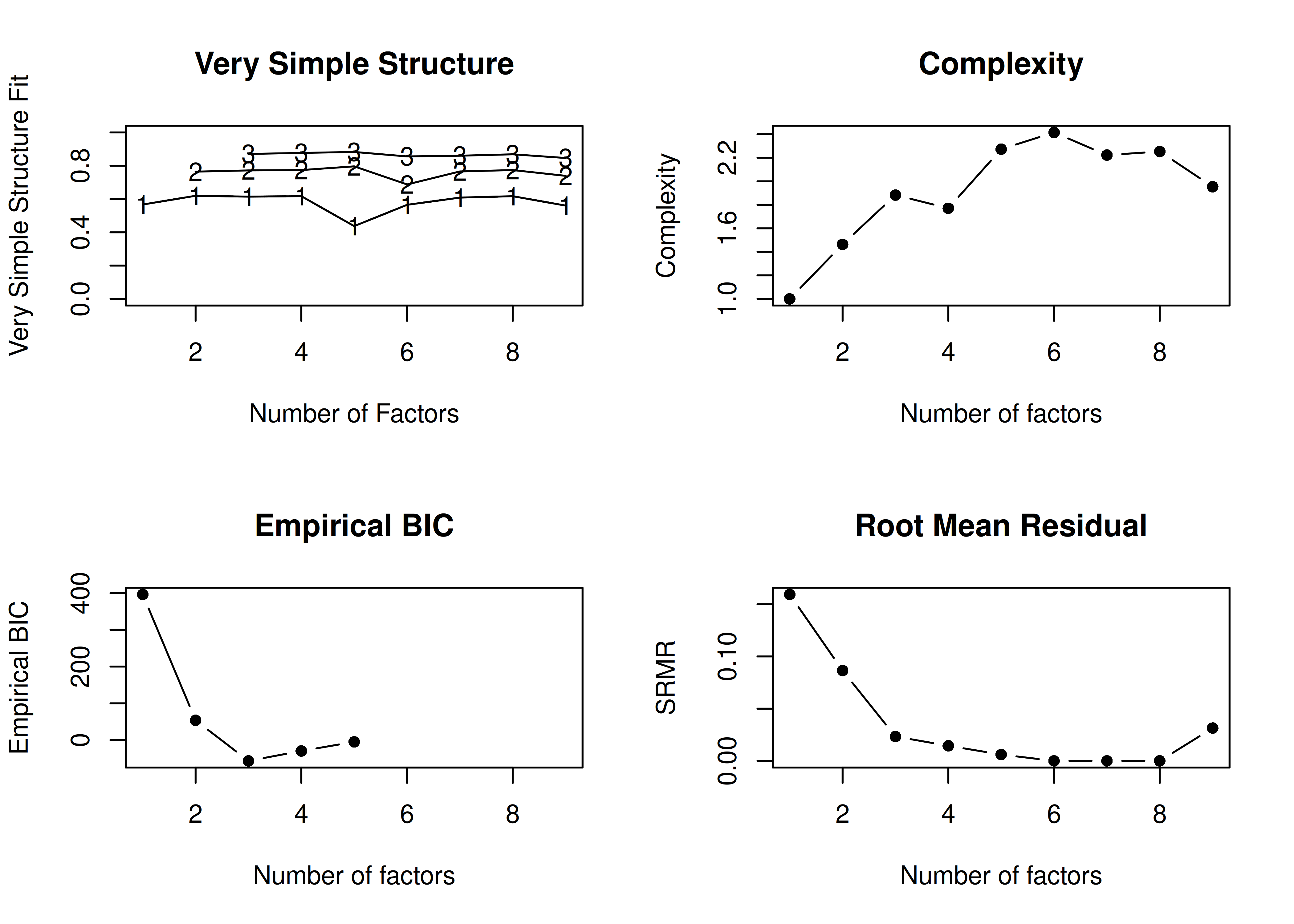
Figure 14.35: Very Simple Structure-Related Indices With no Rotation in Exploratory Factor Analysis.
Number of factors
Call: vss(x = x, n = n, rotate = rotate, diagonal = diagonal, fm = fm,
    n.obs = n.obs, plot = FALSE, title = title, use = use, cor = cor)
VSS complexity 1 achieves a maximimum of 0.62  with  2  factors
VSS complexity 2 achieves a maximimum of 0.8  with  5  factors
The Velicer MAP achieves a minimum of 0.07  with  2  factors
Empirical BIC achieves a minimum of  -56.69  with  3  factors
Sample Size adjusted BIC achieves a minimum of  -5.65  with  4  factors

Statistics by number of factors
  vss1 vss2   map dof   chisq    prob sqresid  fit RMSEA   BIC  SABIC complex
1 0.57 0.00 0.078  27 3.2e+02 2.3e-52     7.1 0.57 0.191 168.4 254.05     1.0
2 0.62 0.76 0.067  19 1.4e+02 1.2e-20     3.9 0.76 0.146  32.5  92.75     1.5
3 0.61 0.77 0.071  12 3.6e+01 3.4e-04     2.1 0.87 0.081 -32.6   5.45     1.9
4 0.62 0.77 0.125   6 9.6e+00 1.4e-01     2.0 0.88 0.044 -24.7  -5.65     1.8
5 0.44 0.80 0.199   1 1.8e+00 1.8e-01     1.6 0.90 0.050  -3.9  -0.77     2.3
6 0.57 0.69 0.403  -3 2.6e-08      NA     1.6 0.91    NA    NA     NA     2.4
7 0.61 0.77 0.447  -6 5.2e-13      NA     1.4 0.91    NA    NA     NA     2.2
8 0.62 0.77 1.000  -8 0.0e+00      NA     1.3 0.92    NA    NA     NA     2.3
9 0.56 0.74    NA  -9 4.4e+01      NA     2.5 0.85    NA    NA     NA     2.0
   eChisq    SRMR eCRMS  eBIC
1 5.5e+02 1.6e-01 0.184 396.3
2 1.6e+02 8.7e-02 0.119  53.8
3 1.2e+01 2.3e-02 0.040 -56.7
4 4.5e+00 1.4e-02 0.035 -29.7
5 8.0e-01 6.1e-03 0.036  -4.9
6 1.3e-08 7.7e-07    NA    NA
7 2.1e-13 3.1e-09    NA    NA
8 2.1e-16 1.0e-10    NA    NA
9 2.1e+01 3.1e-02    NA    NA
14.4.1.2 Run factor analysis
Exploratory factor analysis (EFA) models were fit using the fa() function of the psych package (Revelle, 2022) and the sem() and efa() functions of the lavaan package (Rosseel et al., 2022).
14.4.1.2.1 Orthogonal (Varimax) rotation
14.4.1.2.1.1 psych
Fit a different model with each number of possible factors:
Code
efa1factorOrthogonal <- fa(
  r = HolzingerSwineford1939[,vars],
  nfactors = 1,
  rotate = "varimax",
  fm = "ml")

efa2factorOrthogonal <- fa(
  r = HolzingerSwineford1939[,vars],
  nfactors = 2,
  rotate = "varimax",
  fm = "ml")

efa3factorOrthogonal <- fa(
  r = HolzingerSwineford1939[,vars],
  nfactors = 3,
  rotate = "varimax",
  fm = "ml")

efa4factorOrthogonal <- fa(
  r = HolzingerSwineford1939[,vars],
  nfactors = 4,
  rotate = "varimax",
  fm = "ml")

efa5factorOrthogonal <- fa(
  r = HolzingerSwineford1939[,vars],
  nfactors = 5,
  rotate = "varimax",
  fm = "ml")

efa6factorOrthogonal <- fa(
  r = HolzingerSwineford1939[,vars],
  nfactors = 6,
  rotate = "varimax",
  fm = "ml")

efa7factorOrthogonal <- fa(
  r = HolzingerSwineford1939[,vars],
  nfactors = 7,
  rotate = "varimax",
  fm = "ml")

efa8factorOrthogonal <- fa(
  r = HolzingerSwineford1939[,vars],
  nfactors = 8,
  rotate = "varimax",
  fm = "ml")

efa9factorOrthogonal <- fa(
  r = HolzingerSwineford1939[,vars],
  nfactors = 9,
  rotate = "varimax",
  fm = "ml")
14.4.1.2.1.2 lavaan
Model syntax is specified below:
Code
efa1factorLavaan_syntax <- '
 # EFA Factor Loadings
 efa("efa1")*f1 =~ x1 + x2 + x3 + x4 + x5 + x6 + x7 + x8 + x9
'

efa2factorLavaan_syntax <- '
 # EFA Factor Loadings
 efa("efa1")*f1 +
 efa("efa1")*f2 =~ x1 + x2 + x3 + x4 + x5 + x6 + x7 + x8 + x9
'

efa3factorLavaan_syntax <- '
 # EFA Factor Loadings
 efa("efa1")*f1 +
 efa("efa1")*f2 +
 efa("efa1")*f3 =~ x1 + x2 + x3 + x4 + x5 + x6 + x7 + x8 + x9
'

efa4factorLavaan_syntax <- '
 # EFA Factor Loadings
 efa("efa1")*f1 +
 efa("efa1")*f2 +
 efa("efa1")*f3 +
 efa("efa1")*f4 =~ x1 + x2 + x3 + x4 + x5 + x6 + x7 + x8 + x9
'

efa5factorLavaan_syntax <- '
 # EFA Factor Loadings
 efa("efa1")*f1 +
 efa("efa1")*f2 +
 efa("efa1")*f3 +
 efa("efa1")*f4 +
 efa("efa1")*f5 =~ x1 + x2 + x3 + x4 + x5 + x6 + x7 + x8 + x9
'

efa6factorLavaan_syntax <- '
 # EFA Factor Loadings
 efa("efa1")*f1 +
 efa("efa1")*f2 +
 efa("efa1")*f3 +
 efa("efa1")*f4 +
 efa("efa1")*f5 +
 efa("efa1")*f6 =~ x1 + x2 + x3 + x4 + x5 + x6 + x7 + x8 + x9
'

efa7factorLavaan_syntax <- '
 # EFA Factor Loadings
 efa("efa1")*f1 +
 efa("efa1")*f2 +
 efa("efa1")*f3 +
 efa("efa1")*f4 +
 efa("efa1")*f5 +
 efa("efa1")*f6 +
 efa("efa1")*f7 =~ x1 + x2 + x3 + x4 + x5 + x6 + x7 + x8 + x9
'

efa8factorLavaan_syntax <- '
 # EFA Factor Loadings
 efa("efa1")*f1 +
 efa("efa1")*f2 +
 efa("efa1")*f3 +
 efa("efa1")*f4 +
 efa("efa1")*f5 +
 efa("efa1")*f6 +
 efa("efa1")*f7 +
 efa("efa1")*f8 =~ x1 + x2 + x3 + x4 + x5 + x6 + x7 + x8 + x9
'

efa9factorLavaan_syntax <- '
 # EFA Factor Loadings
 efa("efa1")*f1 +
 efa("efa1")*f2 +
 efa("efa1")*f3 +
 efa("efa1")*f4 +
 efa("efa1")*f5 +
 efa("efa1")*f6 +
 efa("efa1")*f7 +
 efa("efa1")*f8 +
 efa("efa1")*f9 =~ x1 + x2 + x3 + x4 + x5 + x6 + x7 + x8 + x9
'
The models are fitted below:
Code
efa1factorOrthogonalLavaan_fit <- sem(
  efa1factorLavaan_syntax,
  data = HolzingerSwineford1939,
  information = "observed",
  missing = "ML",
  estimator = "MLR",
  rotation = "varimax",
  meanstructure = TRUE,
  rotation.args = list(orthogonal = TRUE))

efa2factorOrthogonalLavaan_fit <- sem(
  efa2factorLavaan_syntax,
  data = HolzingerSwineford1939,
  information = "observed",
  missing = "ML",
  estimator = "MLR",
  rotation = "varimax",
  meanstructure = TRUE,
  rotation.args = list(orthogonal = TRUE))

efa3factorOrthogonalLavaan_fit <- sem(
  efa3factorLavaan_syntax,
  data = HolzingerSwineford1939,
  information = "observed",
  missing = "ML",
  estimator = "MLR",
  rotation = "varimax",
  meanstructure = TRUE,
  rotation.args = list(orthogonal = TRUE))

efa4factorOrthogonalLavaan_fit <- sem(
  efa4factorLavaan_syntax,
  data = HolzingerSwineford1939,
  information = "observed",
  missing = "ML",
  estimator = "MLR",
  rotation = "varimax",
  meanstructure = TRUE,
  rotation.args = list(orthogonal = TRUE))

efa5factorOrthogonalLavaan_fit <- sem(
  efa5factorLavaan_syntax,
  data = HolzingerSwineford1939,
  information = "observed",
  missing = "ML",
  estimator = "MLR",
  rotation = "varimax",
  meanstructure = TRUE,
  rotation.args = list(orthogonal = TRUE))

efa6factorOrthogonalLavaan_fit <- sem(
  efa6factorLavaan_syntax,
  data = HolzingerSwineford1939,
  information = "observed",
  missing = "ML",
  estimator = "MLR",
  rotation = "varimax",
  meanstructure = TRUE,
  rotation.args = list(orthogonal = TRUE))

efa7factorOrthogonalLavaan_fit <- sem(
  efa7factorLavaan_syntax,
  data = HolzingerSwineford1939,
  information = "observed",
  missing = "ML",
  estimator = "MLR",
  rotation = "varimax",
  meanstructure = TRUE,
  rotation.args = list(orthogonal = TRUE))

efa8factorOrthogonalLavaan_fit <- sem(
  efa8factorLavaan_syntax,
  data = HolzingerSwineford1939,
  information = "observed",
  missing = "ML",
  estimator = "MLR",
  rotation = "varimax",
  meanstructure = TRUE,
  rotation.args = list(orthogonal = TRUE))

efa9factorOrthogonalLavaan_fit <- sem(
  efa9factorLavaan_syntax,
  data = HolzingerSwineford1939,
  information = "observed",
  missing = "ML",
  estimator = "MLR",
  rotation = "varimax",
  meanstructure = TRUE,
  rotation.args = list(orthogonal = TRUE))
The efa() wrapper can fit multiple orthogonal EFA models in one function call:
Code
The efa() wrapper can also fit individual orthogonal EFA models (with output = "lavaan"):
Code
efaFactor1OrthogonalLavaan_fit <- efa(
  data = HolzingerSwineford1939,
  ov.names = vars,
  nfactors = 1,
  rotation = "varimax",
  missing = "ML",
  estimator = "MLR",
  meanstructure = TRUE,
  rotation.args = list(orthogonal = TRUE),
  output = "lavaan"
)

efaFactor2OrthogonalLavaan_fit <- efa(
  data = HolzingerSwineford1939,
  ov.names = vars,
  nfactors = 2,
  rotation = "varimax",
  missing = "ML",
  estimator = "MLR",
  meanstructure = TRUE,
  rotation.args = list(orthogonal = TRUE),
  output = "lavaan"
)

efaFactor3OrthogonalLavaan_fit <- efa(
  data = HolzingerSwineford1939,
  ov.names = vars,
  nfactors = 3,
  rotation = "varimax",
  missing = "ML",
  estimator = "MLR",
  meanstructure = TRUE,
  rotation.args = list(orthogonal = TRUE),
  output = "lavaan"
)

efaFactor4OrthogonalLavaan_fit <- efa(
  data = HolzingerSwineford1939,
  ov.names = vars,
  nfactors = 4,
  rotation = "varimax",
  missing = "ML",
  estimator = "MLR",
  meanstructure = TRUE,
  rotation.args = list(orthogonal = TRUE),
  output = "lavaan"
)

efaFactor5OrthogonalLavaan_fit <- efa(
  data = HolzingerSwineford1939,
  ov.names = vars,
  nfactors = 5,
  rotation = "varimax",
  missing = "ML",
  estimator = "MLR",
  meanstructure = TRUE,
  rotation.args = list(orthogonal = TRUE),
  output = "lavaan"
)
14.4.1.2.2 Oblique (Oblimin) rotation
14.4.1.2.2.1 psych
Fit a different model with each number of possible factors:
Code
efa1factorOblique <- fa(
  r = HolzingerSwineford1939[,vars],
  nfactors = 1,
  rotate = "oblimin",
  fm = "ml")

efa2factorOblique <- fa(
  r = HolzingerSwineford1939[,vars],
  nfactors = 2,
  rotate = "oblimin",
  fm = "ml")

efa3factorOblique <- fa(
  r = HolzingerSwineford1939[,vars],
  nfactors = 3,
  rotate = "oblimin",
  fm = "ml")

efa4factorOblique <- fa(
  r = HolzingerSwineford1939[,vars],
  nfactors = 4,
  rotate = "oblimin",
  fm = "ml")

efa5factorOblique <- fa(
  r = HolzingerSwineford1939[,vars],
  nfactors = 5,
  rotate = "oblimin",
  fm = "ml")

efa6factorOblique <- fa(
  r = HolzingerSwineford1939[,vars],
  nfactors = 6,
  rotate = "oblimin",
  fm = "ml")

efa7factorOblique <- fa(
  r = HolzingerSwineford1939[,vars],
  nfactors = 7,
  rotate = "oblimin",
  fm = "ml")

efa8factorOblique <- fa(
  r = HolzingerSwineford1939[,vars],
  nfactors = 8,
  rotate = "oblimin",
  fm = "ml") #no convergence

efa9factorOblique <- fa(
  r = HolzingerSwineford1939[,vars],
  nfactors = 9,
  rotate = "oblimin",
  fm = "ml")
14.4.1.2.2.2 lavaan
The models are fitted below:
Code
# settings to mimic Mplus
mplusRotationArgs <-
  list(
    rstarts = 30,
    row.weights = "none",
    algorithm = "gpa",
    orthogonal = FALSE,
    jac.init.rot = TRUE,
    std.ov = TRUE, # row standard = correlation
    geomin.epsilon = 0.0001)

efa1factorObliqueLavaan_fit <- sem(
  efa1factorLavaan_syntax,
  data = HolzingerSwineford1939,
  information = "observed",
  missing = "ML",
  estimator = "MLR",
  rotation = "geomin",
  meanstructure = TRUE,
  rotation.args = mplusRotationArgs)

efa2factorObliqueLavaan_fit <- sem(
  efa2factorLavaan_syntax,
  data = HolzingerSwineford1939,
  information = "observed",
  missing = "ML",
  estimator = "MLR",
  rotation = "geomin",
  meanstructure = TRUE,
  rotation.args = mplusRotationArgs)

efa3factorObliqueLavaan_fit <- sem(
  efa3factorLavaan_syntax,
  data = HolzingerSwineford1939,
  information = "observed",
  missing = "ML",
  estimator = "MLR",
  rotation = "geomin",
  meanstructure = TRUE,
  rotation.args = mplusRotationArgs)

efa4factorObliqueLavaan_fit <- sem(
  efa4factorLavaan_syntax,
  data = HolzingerSwineford1939,
  information = "observed",
  missing = "ML",
  estimator = "MLR",
  rotation = "geomin",
  meanstructure = TRUE,
  rotation.args = mplusRotationArgs)

efa5factorObliqueLavaan_fit <- sem(
  efa5factorLavaan_syntax,
  data = HolzingerSwineford1939,
  information = "observed",
  missing = "ML",
  estimator = "MLR",
  rotation = "geomin",
  meanstructure = TRUE,
  rotation.args = mplusRotationArgs)

efa6factorObliqueLavaan_fit <- sem(
  efa6factorLavaan_syntax,
  data = HolzingerSwineford1939,
  information = "observed",
  missing = "ML",
  estimator = "MLR",
  rotation = "geomin",
  meanstructure = TRUE,
  rotation.args = mplusRotationArgs)

efa7factorObliqueLavaan_fit <- sem(
  efa7factorLavaan_syntax,
  data = HolzingerSwineford1939,
  information = "observed",
  missing = "ML",
  estimator = "MLR",
  rotation = "geomin",
  meanstructure = TRUE,
  rotation.args = mplusRotationArgs)

efa8factorObliqueLavaan_fit <- sem(
  efa8factorLavaan_syntax,
  data = HolzingerSwineford1939,
  information = "observed",
  missing = "ML",
  estimator = "MLR",
  rotation = "geomin",
  meanstructure = TRUE,
  rotation.args = mplusRotationArgs)

efa9factorObliqueLavaan_fit <- sem(
  efa9factorLavaan_syntax,
  data = HolzingerSwineford1939,
  information = "observed",
  missing = "ML",
  estimator = "MLR",
  rotation = "geomin",
  meanstructure = TRUE,
  rotation.args = mplusRotationArgs)
The efa() wrapper can fit multiple oblique EFA models in one function call:
Code
The efa() wrapper can also fit individual oblique EFA models (with output = "lavaan"):
Code
efaFactor1ObliqueLavaan_fit <- efa(
  data = HolzingerSwineford1939,
  ov.names = vars,
  nfactors = 1,
  rotation = "geomin",
  missing = "ML",
  estimator = "MLR",
  meanstructure = TRUE,
  rotation.args = mplusRotationArgs,
  output = "lavaan"
)

efaFactor2ObliqueLavaan_fit <- efa(
  data = HolzingerSwineford1939,
  ov.names = vars,
  nfactors = 2,
  rotation = "geomin",
  missing = "ML",
  estimator = "MLR",
  meanstructure = TRUE,
  rotation.args = mplusRotationArgs,
  output = "lavaan"
)

efaFactor3ObliqueLavaan_fit <- efa(
  data = HolzingerSwineford1939,
  ov.names = vars,
  nfactors = 3,
  rotation = "geomin",
  missing = "ML",
  estimator = "MLR",
  meanstructure = TRUE,
  rotation.args = mplusRotationArgs,
  output = "lavaan"
)

efaFactor4ObliqueLavaan_fit <- efa(
  data = HolzingerSwineford1939,
  ov.names = vars,
  nfactors = 4,
  rotation = "geomin",
  missing = "ML",
  estimator = "MLR",
  meanstructure = TRUE,
  rotation.args = mplusRotationArgs,
  output = "lavaan"
)

efaFactor5ObliqueLavaan_fit <- efa(
  data = HolzingerSwineford1939,
  ov.names = vars,
  nfactors = 5,
  rotation = "geomin",
  missing = "ML",
  estimator = "MLR",
  meanstructure = TRUE,
  rotation.args = mplusRotationArgs,
  output = "lavaan"
)
14.4.1.3 Factor Loadings
14.4.1.3.1 Orthogonal (Varimax) rotation
14.4.1.3.1.1 psych
The factor loadings and summaries of the model results are below:
Factor Analysis using method =  ml
Call: fa(r = HolzingerSwineford1939[, vars], nfactors = 1, rotate = "varimax",
    fm = "ml")
Standardized loadings (pattern matrix) based upon correlation matrix
    ML1    h2   u2 com
x1 0.45 0.202 0.80   1
x2 0.24 0.056 0.94   1
x3 0.27 0.071 0.93   1
x4 0.84 0.710 0.29   1
x5 0.85 0.722 0.28   1
x6 0.80 0.636 0.36   1
x7 0.17 0.029 0.97   1
x8 0.26 0.068 0.93   1
x9 0.32 0.099 0.90   1

                ML1
SS loadings    2.59
Proportion Var 0.29

Mean item complexity =  1
Test of the hypothesis that 1 factor is sufficient.

df null model =  36  with the objective function =  3.05 with Chi Square =  904.68
df of  the model are 27  and the objective function was  1.09

The root mean square of the residuals (RMSR) is  0.16
The df corrected root mean square of the residuals is  0.18

The harmonic n.obs is  222 with the empirical chi square  406.89  with prob <  2e-69
The total n.obs was  301  with Likelihood Chi Square =  322.51  with prob <  2.3e-52

Tucker Lewis Index of factoring reliability =  0.545
RMSEA index =  0.191  and the 90 % confidence intervals are  0.173 0.21
BIC =  168.42
Fit based upon off diagonal values = 0.75
Measures of factor score adequacy
                                                   ML1
Correlation of (regression) scores with factors   0.94
Multiple R square of scores with factors          0.88
Minimum correlation of possible factor scores 0.76Factor Analysis using method = ml
Call: fa(r = HolzingerSwineford1939[, vars], nfactors = 2, rotate = "varimax",
fm = "ml")
Standardized loadings (pattern matrix) based upon correlation matrix
ML1 ML2 h2 u2 com
x1 0.34 0.43 0.301 0.70 1.9
x2 0.17 0.25 0.092 0.91 1.7
x3 0.13 0.48 0.252 0.75 1.1
x4 0.85 0.14 0.737 0.26 1.1
x5 0.83 0.19 0.726 0.27 1.1
x6 0.79 0.15 0.643 0.36 1.1
x7 0.05 0.44 0.198 0.80 1.0
x8 0.09 0.62 0.388 0.61 1.0
x9 0.11 0.75 0.576 0.42 1.0
ML1 ML2
SS loadings 2.22 1.70
Proportion Var 0.25 0.19
Cumulative Var 0.25 0.43
Proportion Explained 0.57 0.43
Cumulative Proportion 0.57 1.00
Mean item complexity = 1.2
Test of the hypothesis that 2 factors are sufficient.
df null model = 36 with the objective function = 3.05 with Chi Square = 904.68
df of the model are 19 and the objective function was 0.48
The root mean square of the residuals (RMSR) is 0.09
The df corrected root mean square of the residuals is 0.12
The harmonic n.obs is 222 with the empirical chi square 120.59 with prob < 8.6e-17
The total n.obs was 301 with Likelihood Chi Square = 140.93 with prob < 1.2e-20
Tucker Lewis Index of factoring reliability = 0.733
RMSEA index = 0.146 and the 90 % confidence intervals are 0.124 0.169
BIC = 32.49
Fit based upon off diagonal values = 0.93
Measures of factor score adequacy
ML1 ML2
Correlation of (regression) scores with factors 0.93 0.85
Multiple R square of scores with factors 0.86 0.72
Minimum correlation of possible factor scores 0.73 0.45Factor Analysis using method = ml
Call: fa(r = HolzingerSwineford1939[, vars], nfactors = 3, rotate = "varimax",
fm = "ml")
Standardized loadings (pattern matrix) based upon correlation matrix
ML1 ML3 ML2 h2 u2 com
x1 0.28 0.61 0.13 0.47 0.53 1.5
x2 0.11 0.49 -0.04 0.26 0.74 1.1
x3 0.05 0.69 0.16 0.50 0.50 1.1
x4 0.83 0.17 0.08 0.73 0.27 1.1
x5 0.84 0.14 0.13 0.74 0.26 1.1
x6 0.78 0.17 0.09 0.64 0.36 1.1
x7 0.07 -0.08 0.69 0.49 0.51 1.1
x8 0.10 0.17 0.71 0.54 0.46 1.2
x9 0.11 0.42 0.54 0.48 0.52 2.0
ML1 ML3 ML2
SS loadings 2.12 1.38 1.35
Proportion Var 0.24 0.15 0.15
Cumulative Var 0.24 0.39 0.54
Proportion Explained 0.44 0.28 0.28
Cumulative Proportion 0.44 0.72 1.00
Mean item complexity = 1.3
Test of the hypothesis that 3 factors are sufficient.
df null model = 36 with the objective function = 3.05 with Chi Square = 904.68
df of the model are 12 and the objective function was 0.12
The root mean square of the residuals (RMSR) is 0.02
The df corrected root mean square of the residuals is 0.04
The harmonic n.obs is 222 with the empirical chi square 8.6 with prob < 0.74
The total n.obs was 301 with Likelihood Chi Square = 35.88 with prob < 0.00034
Tucker Lewis Index of factoring reliability = 0.917
RMSEA index = 0.081 and the 90 % confidence intervals are 0.052 0.113
BIC = -32.61
Fit based upon off diagonal values = 0.99
Measures of factor score adequacy
ML1 ML3 ML2
Correlation of (regression) scores with factors 0.93 0.82 0.84
Multiple R square of scores with factors 0.86 0.67 0.71
Minimum correlation of possible factor scores 0.71 0.34 0.41Factor Analysis using method = ml
Call: fa(r = HolzingerSwineford1939[, vars], nfactors = 4, rotate = "varimax",
fm = "ml")
Standardized loadings (pattern matrix) based upon correlation matrix
ML1 ML4 ML3 ML2 h2 u2 com
x1 0.26 0.63 0.13 0.13 0.50 0.499 1.5
x2 0.11 0.50 -0.04 -0.08 0.27 0.734 1.2
x3 0.05 0.67 0.17 0.02 0.48 0.522 1.1
x4 0.89 0.17 0.08 0.40 1.00 0.005 1.5
x5 0.93 0.14 0.13 -0.32 1.00 0.005 1.3
x6 0.71 0.19 0.10 0.01 0.55 0.449 1.2
x7 0.07 -0.10 0.74 0.12 0.58 0.417 1.1
x8 0.08 0.19 0.68 -0.07 0.52 0.484 1.2
x9 0.12 0.42 0.53 -0.07 0.48 0.520 2.1
ML1 ML4 ML3 ML2
SS loadings 2.27 1.41 1.38 0.31
Proportion Var 0.25 0.16 0.15 0.03
Cumulative Var 0.25 0.41 0.56 0.60
Proportion Explained 0.42 0.26 0.26 0.06
Cumulative Proportion 0.42 0.68 0.94 1.00
Mean item complexity = 1.4
Test of the hypothesis that 4 factors are sufficient.
df null model = 36 with the objective function = 3.05 with Chi Square = 904.68
df of the model are 6 and the objective function was 0.03
The root mean square of the residuals (RMSR) is 0.01
The df corrected root mean square of the residuals is 0.04
The harmonic n.obs is 222 with the empirical chi square 3.28 with prob < 0.77
The total n.obs was 301 with Likelihood Chi Square = 9.57 with prob < 0.14
Tucker Lewis Index of factoring reliability = 0.975
RMSEA index = 0.044 and the 90 % confidence intervals are 0 0.095
BIC = -24.67
Fit based upon off diagonal values = 1
Measures of factor score adequacy
ML1 ML4 ML3 ML2
Correlation of (regression) scores with factors 0.99 0.83 0.85 0.99
Multiple R square of scores with factors 0.99 0.68 0.73 0.98
Minimum correlation of possible factor scores 0.97 0.36 0.46 0.96Factor Analysis using method = ml
Call: fa(r = HolzingerSwineford1939[, vars], nfactors = 5, rotate = "varimax",
fm = "ml")
Standardized loadings (pattern matrix) based upon correlation matrix
ML1 ML4 ML5 ML2 ML3 h2 u2 com
x1 0.28 0.61 0.02 0.13 -0.15 0.49 0.505 1.6
x2 0.11 0.48 -0.11 0.05 0.06 0.26 0.739 1.3
x3 0.04 0.72 0.14 0.01 0.00 0.54 0.455 1.1
x4 0.89 0.17 0.12 -0.03 -0.31 0.94 0.061 1.4
x5 0.91 0.14 0.05 0.09 0.36 1.00 0.005 1.4
x6 0.72 0.19 0.04 0.08 0.00 0.56 0.437 1.2
x7 0.07 -0.04 0.74 0.22 -0.03 0.60 0.396 1.2
x8 0.09 0.18 0.40 0.89 0.01 1.00 0.005 1.5
x9 0.12 0.46 0.42 0.23 0.12 0.46 0.535 2.8
ML1 ML4 ML5 ML2 ML3
SS loadings 2.27 1.45 0.94 0.93 0.27
Proportion Var 0.25 0.16 0.10 0.10 0.03
Cumulative Var 0.25 0.41 0.52 0.62 0.65
Proportion Explained 0.39 0.25 0.16 0.16 0.05
Cumulative Proportion 0.39 0.64 0.80 0.95 1.00
Mean item complexity = 1.5
Test of the hypothesis that 5 factors are sufficient.
df null model = 36 with the objective function = 3.05 with Chi Square = 904.68
df of the model are 1 and the objective function was 0.01
The root mean square of the residuals (RMSR) is 0.01
The df corrected root mean square of the residuals is 0.04
The harmonic n.obs is 222 with the empirical chi square 0.55 with prob < 0.46
The total n.obs was 301 with Likelihood Chi Square = 1.77 with prob < 0.18
Tucker Lewis Index of factoring reliability = 0.968
RMSEA index = 0.05 and the 90 % confidence intervals are 0 0.172
BIC = -3.94
Fit based upon off diagonal values = 1
Measures of factor score adequacy
ML1 ML4 ML5 ML2 ML3
Correlation of (regression) scores with factors 0.99 0.84 0.78 0.95 0.93
Multiple R square of scores with factors 0.97 0.70 0.60 0.91 0.87
Minimum correlation of possible factor scores 0.94 0.40 0.20 0.82 0.73Factor Analysis using method = ml
Call: fa(r = HolzingerSwineford1939[, vars], nfactors = 6, rotate = "varimax",
fm = "ml")
Standardized loadings (pattern matrix) based upon correlation matrix
ML1 ML4 ML2 ML6 ML3 ML5 h2 u2 com
x1 0.25 0.61 0.13 0.20 0.14 -0.03 0.51 0.489 1.8
x2 0.11 0.47 -0.04 -0.04 0.09 0.05 0.25 0.748 1.2
x3 0.05 0.75 0.15 -0.03 -0.18 -0.06 0.63 0.374 1.2
x4 0.84 0.17 0.08 0.44 -0.06 -0.03 0.94 0.060 1.6
x5 0.90 0.15 0.12 -0.11 0.05 0.32 0.95 0.049 1.4
x6 0.79 0.18 0.09 -0.06 0.04 -0.19 0.70 0.298 1.3
x7 0.07 -0.09 0.75 0.07 -0.21 -0.04 0.62 0.376 1.2
x8 0.09 0.18 0.75 -0.05 0.28 -0.01 0.68 0.321 1.4
x9 0.10 0.43 0.51 -0.01 -0.01 0.13 0.47 0.530 2.2
ML1 ML4 ML2 ML6 ML3 ML5
SS loadings 2.23 1.47 1.45 0.25 0.19 0.16
Proportion Var 0.25 0.16 0.16 0.03 0.02 0.02
Cumulative Var 0.25 0.41 0.57 0.60 0.62 0.64
Proportion Explained 0.39 0.25 0.25 0.04 0.03 0.03
Cumulative Proportion 0.39 0.64 0.89 0.94 0.97 1.00
Mean item complexity = 1.5
Test of the hypothesis that 6 factors are sufficient.
df null model = 36 with the objective function = 3.05 with Chi Square = 904.68
df of the model are -3 and the objective function was 0
The root mean square of the residuals (RMSR) is 0
The df corrected root mean square of the residuals is NA
The harmonic n.obs is 222 with the empirical chi square 0 with prob < NA
The total n.obs was 301 with Likelihood Chi Square = 0 with prob < NA
Tucker Lewis Index of factoring reliability = 1.042
Fit based upon off diagonal values = 1
Measures of factor score adequacy
ML1 ML4 ML2 ML6 ML3
Correlation of (regression) scores with factors 0.96 0.85 0.88 0.81 0.58
Multiple R square of scores with factors 0.93 0.73 0.78 0.66 0.34
Minimum correlation of possible factor scores 0.86 0.45 0.55 0.32 -0.32
ML5
Correlation of (regression) scores with factors 0.68
Multiple R square of scores with factors 0.46
Minimum correlation of possible factor scores -0.07Factor Analysis using method = ml
Call: fa(r = HolzingerSwineford1939[, vars], nfactors = 7, rotate = "varimax",
fm = "ml")
Standardized loadings (pattern matrix) based upon correlation matrix
ML1 ML3 ML4 ML7 ML5 ML2 ML6 h2 u2 com
x1 0.24 0.12 0.50 0.58 0.06 0.00 0.01 0.66 0.3413 2.4
x2 0.12 -0.04 0.52 0.06 -0.01 0.02 0.19 0.33 0.6697 1.4
x3 0.06 0.16 0.70 0.14 0.02 -0.03 -0.19 0.57 0.4300 1.4
x4 0.83 0.09 0.10 0.20 0.50 -0.02 -0.02 0.99 0.0058 1.8
x5 0.91 0.12 0.13 0.02 -0.09 0.32 0.06 0.99 0.0146 1.4
x6 0.79 0.09 0.15 0.08 -0.04 -0.20 -0.01 0.70 0.2999 1.3
x7 0.06 0.69 -0.07 -0.04 0.10 -0.02 -0.14 0.52 0.4786 1.2
x8 0.09 0.77 0.13 0.14 -0.10 -0.03 0.19 0.69 0.3135 1.3
x9 0.11 0.53 0.41 0.09 0.00 0.13 -0.07 0.49 0.5133 2.2
ML1 ML3 ML4 ML7 ML5 ML2 ML6
SS loadings 2.24 1.43 1.24 0.44 0.28 0.16 0.14
Proportion Var 0.25 0.16 0.14 0.05 0.03 0.02 0.02
Cumulative Var 0.25 0.41 0.55 0.59 0.63 0.64 0.66
Proportion Explained 0.38 0.24 0.21 0.07 0.05 0.03 0.02
Cumulative Proportion 0.38 0.62 0.83 0.90 0.95 0.98 1.00
Mean item complexity = 1.6
Test of the hypothesis that 7 factors are sufficient.
df null model = 36 with the objective function = 3.05 with Chi Square = 904.68
df of the model are -6 and the objective function was 0
The root mean square of the residuals (RMSR) is 0
The df corrected root mean square of the residuals is NA
The harmonic n.obs is 222 with the empirical chi square 0 with prob < NA
The total n.obs was 301 with Likelihood Chi Square = 0 with prob < NA
Tucker Lewis Index of factoring reliability = 1.042
Fit based upon off diagonal values = 1
Measures of factor score adequacy
ML1 ML3 ML4 ML7 ML5
Correlation of (regression) scores with factors 0.97 0.87 0.80 0.65 0.89
Multiple R square of scores with factors 0.94 0.76 0.64 0.42 0.79
Minimum correlation of possible factor scores 0.88 0.52 0.28 -0.16 0.59
ML2 ML6
Correlation of (regression) scores with factors 0.70 0.47
Multiple R square of scores with factors 0.50 0.22
Minimum correlation of possible factor scores -0.01 -0.55Factor Analysis using method = ml
Call: fa(r = HolzingerSwineford1939[, vars], nfactors = 8, rotate = "varimax",
fm = "ml")
Standardized loadings (pattern matrix) based upon correlation matrix
ML1 ML3 ML4 ML7 ML6 ML2 ML5 ML8 h2 u2 com
x1 0.23 0.12 0.44 0.62 0.07 0.05 0.00 0.01 0.65 0.3462 2.3
x2 0.11 -0.03 0.57 0.07 0.01 0.00 0.02 -0.10 0.36 0.6438 1.2
x3 0.06 0.14 0.60 0.24 0.18 0.01 -0.05 0.25 0.54 0.4648 2.1
x4 0.82 0.08 0.08 0.22 0.02 0.50 -0.02 0.02 0.99 0.0140 1.9
x5 0.92 0.10 0.13 0.03 0.13 -0.10 0.29 -0.06 0.99 0.0091 1.3
x6 0.79 0.10 0.15 0.10 -0.02 -0.03 -0.22 0.04 0.71 0.2884 1.3
x7 0.06 0.72 -0.09 -0.04 0.04 0.11 0.01 0.16 0.57 0.4309 1.2
x8 0.10 0.74 0.14 0.14 0.06 -0.10 -0.02 -0.16 0.64 0.3580 1.3
x9 0.11 0.49 0.33 0.12 0.48 0.01 0.02 0.02 0.61 0.3912 3.0
ML1 ML3 ML4 ML7 ML6 ML2 ML5 ML8
SS loadings 2.24 1.37 1.07 0.54 0.29 0.28 0.14 0.13
Proportion Var 0.25 0.15 0.12 0.06 0.03 0.03 0.02 0.01
Cumulative Var 0.25 0.40 0.52 0.58 0.61 0.64 0.66 0.67
Proportion Explained 0.37 0.23 0.18 0.09 0.05 0.05 0.02 0.02
Cumulative Proportion 0.37 0.60 0.77 0.86 0.91 0.96 0.98 1.00
Mean item complexity = 1.7
Test of the hypothesis that 8 factors are sufficient.
df null model = 36 with the objective function = 3.05 with Chi Square = 904.68
df of the model are -8 and the objective function was 0
The root mean square of the residuals (RMSR) is 0
The df corrected root mean square of the residuals is NA
The harmonic n.obs is 222 with the empirical chi square 0 with prob < NA
The total n.obs was 301 with Likelihood Chi Square = 0 with prob < NA
Tucker Lewis Index of factoring reliability = 1.042
Fit based upon off diagonal values = 1
Measures of factor score adequacy
ML1 ML3 ML4 ML7 ML6
Correlation of (regression) scores with factors 0.97 0.86 0.75 0.67 0.55
Multiple R square of scores with factors 0.95 0.74 0.56 0.45 0.30
Minimum correlation of possible factor scores 0.89 0.48 0.12 -0.10 -0.39
ML2 ML5 ML8
Correlation of (regression) scores with factors 0.89 0.67 0.46
Multiple R square of scores with factors 0.79 0.45 0.21
Minimum correlation of possible factor scores 0.59 -0.10 -0.58Factor Analysis using method = ml
Call: fa(r = HolzingerSwineford1939[, vars], nfactors = 9, rotate = "varimax",
fm = "ml")
Standardized loadings (pattern matrix) based upon correlation matrix
ML1 ML3 ML2 ML4 ML6 ML9 ML5 ML7 ML8 h2 u2 com
x1 0.29 0.59 0.14 0.07 0 0 0 0 0 0.45 0.55 1.6
x2 0.11 0.49 -0.03 -0.06 0 0 0 0 0 0.26 0.74 1.1
x3 0.07 0.61 0.18 0.03 0 0 0 0 0 0.41 0.59 1.2
x4 0.81 0.17 0.09 0.04 0 0 0 0 0 0.70 0.30 1.1
x5 0.81 0.15 0.14 -0.03 0 0 0 0 0 0.69 0.31 1.1
x6 0.77 0.17 0.09 -0.01 0 0 0 0 0 0.62 0.38 1.1
x7 0.07 -0.06 0.64 0.03 0 0 0 0 0 0.41 0.59 1.1
x8 0.10 0.18 0.66 -0.02 0 0 0 0 0 0.47 0.53 1.2
x9 0.11 0.40 0.53 -0.02 0 0 0 0 0 0.46 0.54 2.0
ML1 ML3 ML2 ML4 ML6 ML9 ML5 ML7 ML8
SS loadings 2.02 1.24 1.20 0.01 0.0 0.0 0.0 0.0 0.0
Proportion Var 0.22 0.14 0.13 0.00 0.0 0.0 0.0 0.0 0.0
Cumulative Var 0.22 0.36 0.50 0.50 0.5 0.5 0.5 0.5 0.5
Proportion Explained 0.45 0.28 0.27 0.00 0.0 0.0 0.0 0.0 0.0
Cumulative Proportion 0.45 0.73 1.00 1.00 1.0 1.0 1.0 1.0 1.0
Mean item complexity = 1.3
Test of the hypothesis that 9 factors are sufficient.
df null model = 36 with the objective function = 3.05 with Chi Square = 904.68
df of the model are -9 and the objective function was 0.15
The root mean square of the residuals (RMSR) is 0.03
The df corrected root mean square of the residuals is NA
The harmonic n.obs is 222 with the empirical chi square 15.66 with prob < NA
The total n.obs was 301 with Likelihood Chi Square = 43.91 with prob < NA
Tucker Lewis Index of factoring reliability = 1.249
Fit based upon off diagonal values = 0.99
Measures of factor score adequacy
ML1 ML3 ML2 ML4 ML6 ML9
Correlation of (regression) scores with factors 0.90 0.76 0.78 0.14 0 0
Multiple R square of scores with factors 0.81 0.58 0.61 0.02 0 0
Minimum correlation of possible factor scores 0.61 0.17 0.22 -0.96 -1 -1
ML5 ML7 ML8
Correlation of (regression) scores with factors 0 0 0
Multiple R square of scores with factors 0 0 0
Minimum correlation of possible factor scores -1 -1 -114.4.1.3.1.2 lavaan
The factor loadings and summaries of the model results are below:
This is lavaan 0.6-20 -- running exploratory factor analysis

  Estimator                                         ML
  Rotation method                   VARIMAX ORTHOGONAL
  Rotation algorithm (rstarts)                GPA (30)
  Standardized metric                             TRUE
  Row weights                                   Kaiser

  Number of observations                           301
  Number of missing patterns                        75

Overview models:
                    aic      bic    sabic   chisq df pvalue   cfi rmsea
  nfactors = 1 6655.547 6755.639 6670.010 235.316 27  0.000 0.664 0.190
  nfactors = 2 6536.011 6665.760 6554.760 112.999 19  0.000 0.865 0.148
  nfactors = 3 6468.608 6624.307 6491.107  23.723 12  0.022 0.988 0.080
  nfactors = 4 6464.728 6642.669 6490.440   5.251  6  0.512 1.000 0.000
  nfactors = 5 6469.292 6665.769 6497.683   0.365  1  0.546    NA 0.000

Eigenvalues correlation matrix:

    ev1     ev2     ev3     ev4     ev5     ev6     ev7     ev8     ev9
  3.220   1.621   1.380   0.689   0.569   0.542   0.461   0.289   0.229

Number of factors:  1

Standardized loadings: (* = significant at 1% level)

       f1       unique.var   communalities
x1  0.447*           0.800           0.200
x2      .*           0.944           0.056
x3      .*           0.928           0.072
x4  0.829*           0.313           0.687
x5  0.851*           0.276           0.724
x6  0.817*           0.332           0.668
x7      .*           0.964           0.036
x8      .*           0.926           0.074
x9  0.335*           0.888           0.112

                           f1
Sum of squared loadings 2.629
Proportion of total     1.000
Proportion var          0.292
Cumulative var          0.292

Number of factors:  2

Standardized loadings: (* = significant at 1% level)

       f1      f2       unique.var   communalities
x1  0.323*  0.427*           0.714           0.286
x2      .       .            0.907           0.093
x3      .   0.495*           0.742           0.258
x4  0.840*      .            0.279           0.721
x5  0.842*      .*           0.259           0.741
x6  0.796*      .            0.333           0.667
x7          0.438*           0.804           0.196
x8          0.612*           0.619           0.381
x9      .   0.737*           0.441           0.559

                              f1    f2 total
Sum of sq (ortho) loadings 2.215 1.686 3.900
Proportion of total        0.568 0.432 1.000
Proportion var             0.246 0.187 0.433
Cumulative var             0.246 0.433 0.433

Number of factors:  3

Standardized loadings: (* = significant at 1% level)

       f1      f2      f3       unique.var   communalities
x1  0.620*      .*      .            0.531           0.469
x2  0.497*      .                    0.741           0.259
x3  0.689*              .            0.493           0.507
x4      .   0.830*                   0.284           0.716
x5      .   0.854*      .            0.241           0.759
x6      .*  0.782*                   0.336           0.664
x7                  0.706*           0.487           0.513
x8      .           0.689*           0.488           0.512
x9  0.402*      .   0.536*           0.533           0.467

                              f2    f1    f3 total
Sum of sq (ortho) loadings 2.143 1.385 1.338 4.865
Proportion of total        0.440 0.285 0.275 1.000
Proportion var             0.238 0.154 0.149 0.541
Cumulative var             0.238 0.392 0.541 0.541

Number of factors:  4

Standardized loadings: (* = significant at 1% level)

       f1      f2      f3      f4       unique.var   communalities
x1  0.634*              .*      .            0.516           0.484
x2  0.502*                                   0.733           0.267
x3  0.677*                      .*           0.506           0.494
x4      .   0.435   0.886*                   0.000           1.000
x5      .       .   0.943*      .            0.000           1.000
x6      .*          0.718*      .            0.422           0.578
x7      .       .*          0.756*           0.396           0.604
x8      .*                  0.657*           0.521           0.479
x9  0.414*              .*  0.527*           0.522           0.478

                              f3    f1    f4    f2 total
Sum of sq (ortho) loadings 2.293 1.417 1.357 0.317 5.384
Proportion of total        0.426 0.263 0.252 0.059 1.000
Proportion var             0.255 0.157 0.151 0.035 0.598
Cumulative var             0.255 0.412 0.563 0.598 0.598

Number of factors:  5

Standardized loadings: (* = significant at 1% level)

       f1      f2      f3      f4      f5       unique.var   communalities
x1  0.603*      .               .*      .            0.517           0.483
x2  0.473*      .*                                   0.748           0.252
x3  0.462*  0.871*                      .*           0.000           1.000
x4      .           0.444   0.882*                   0.000           1.000
x5      .               .   0.942*      .            0.000           1.000
x6      .*                  0.719*      .            0.423           0.577
x7      .               .           0.761*           0.333           0.667
x8      .                           0.688*           0.475           0.525
x9  0.338*      .               .*  0.534*           0.547           0.453

                              f4    f5    f1    f2    f3 total
Sum of sq (ortho) loadings 2.282 1.418 1.092 0.847 0.316 5.955
Proportion of total        0.383 0.238 0.183 0.142 0.053 1.000
Proportion var             0.254 0.158 0.121 0.094 0.035 0.662
Cumulative var             0.254 0.411 0.533 0.627 0.662 0.662
Code
lavaan 0.6-20 ended normally after 30 iterations

  Estimator                                         ML
  Optimization method                           NLMINB
  Number of model parameters                        27

  Rotation method                   VARIMAX ORTHOGONAL
  Rotation algorithm (rstarts)                GPA (30)
  Standardized metric                             TRUE
  Row weights                                   Kaiser

  Number of observations                           301
  Number of missing patterns                        75

Model Test User Model:
                                              Standard      Scaled
  Test Statistic                               239.990     235.316
  Degrees of freedom                                27          27
  P-value (Chi-square)                           0.000       0.000
  Scaling correction factor                                  1.020
    Yuan-Bentler correction (Mplus variant)

Model Test Baseline Model:

  Test statistic                               693.305     646.574
  Degrees of freedom                                36          36
  P-value                                        0.000       0.000
  Scaling correction factor                                  1.072

User Model versus Baseline Model:

  Comparative Fit Index (CFI)                    0.676       0.659
  Tucker-Lewis Index (TLI)                       0.568       0.545

  Robust Comparative Fit Index (CFI)                         0.664
  Robust Tucker-Lewis Index (TLI)                            0.552

Loglikelihood and Information Criteria:

  Loglikelihood user model (H0)              -3300.774   -3300.774
  Scaling correction factor                                  1.108
      for the MLR correction
  Loglikelihood unrestricted model (H1)      -3180.778   -3180.778
  Scaling correction factor                                  1.064
      for the MLR correction

  Akaike (AIC)                                6655.547    6655.547
  Bayesian (BIC)                              6755.639    6755.639
  Sample-size adjusted Bayesian (SABIC)       6670.010    6670.010

Root Mean Square Error of Approximation:

  RMSEA                                          0.162       0.160
  90 Percent confidence interval - lower         0.143       0.142
  90 Percent confidence interval - upper         0.181       0.179
  P-value H_0: RMSEA <= 0.050                    0.000       0.000
  P-value H_0: RMSEA >= 0.080                    1.000       1.000

  Robust RMSEA                                               0.190
  90 Percent confidence interval - lower                     0.167
  90 Percent confidence interval - upper                     0.214
  P-value H_0: Robust RMSEA <= 0.050                         0.000
  P-value H_0: Robust RMSEA >= 0.080                         1.000

Standardized Root Mean Square Residual:

  SRMR                                           0.129       0.129

Parameter Estimates:

  Standard errors                             Sandwich
  Information bread                           Observed
  Observed information based on                Hessian

Latent Variables:
                   Estimate  Std.Err  z-value  P(>|z|)   Std.lv  Std.all
  f1 =~ efa1
    x1                0.517    0.087    5.944    0.000    0.517    0.447
    x2                0.273    0.083    3.277    0.001    0.273    0.236
    x3                0.303    0.087    3.506    0.000    0.303    0.269
    x4                0.973    0.067   14.475    0.000    0.973    0.829
    x5                1.100    0.066   16.748    0.000    1.100    0.851
    x6                0.851    0.068   12.576    0.000    0.851    0.817
    x7                0.203    0.078    2.590    0.010    0.203    0.189
    x8                0.276    0.077    3.584    0.000    0.276    0.272
    x9                0.341    0.082    4.154    0.000    0.341    0.335

Intercepts:
                   Estimate  Std.Err  z-value  P(>|z|)   Std.lv  Std.all
   .x1                4.961    0.072   69.035    0.000    4.961    4.290
   .x2                6.058    0.071   85.159    0.000    6.058    5.232
   .x3                2.222    0.070   31.650    0.000    2.222    1.971
   .x4                3.098    0.071   43.846    0.000    3.098    2.639
   .x5                4.356    0.078   56.050    0.000    4.356    3.369
   .x6                2.188    0.064   34.213    0.000    2.188    2.101
   .x7                4.173    0.066   63.709    0.000    4.173    3.895
   .x8                5.516    0.063   87.910    0.000    5.516    5.433
   .x9                5.407    0.063   85.469    0.000    5.407    5.303

Variances:
                   Estimate  Std.Err  z-value  P(>|z|)   Std.lv  Std.all
   .x1                1.069    0.116    9.243    0.000    1.069    0.800
   .x2                1.266    0.136    9.282    0.000    1.266    0.944
   .x3                1.179    0.086   13.758    0.000    1.179    0.928
   .x4                0.431    0.062    6.913    0.000    0.431    0.313
   .x5                0.461    0.073    6.349    0.000    0.461    0.276
   .x6                0.360    0.056    6.458    0.000    0.360    0.332
   .x7                1.107    0.085   13.003    0.000    1.107    0.964
   .x8                0.955    0.114    8.347    0.000    0.955    0.926
   .x9                0.923    0.088   10.486    0.000    0.923    0.888
    f1                1.000                               1.000    1.000

R-Square:
                   Estimate
    x1                0.200
    x2                0.056
    x3                0.072
    x4                0.687
    x5                0.724
    x6                0.668
    x7                0.036
    x8                0.074
    x9                0.112
Code
lavaan 0.6-20 ended normally after 37 iterations

  Estimator                                         ML
  Optimization method                           NLMINB
  Number of model parameters                        36
  Row rank of the constraints matrix                 1

  Rotation method                   VARIMAX ORTHOGONAL
  Rotation algorithm (rstarts)                GPA (30)
  Standardized metric                             TRUE
  Row weights                                   Kaiser

  Number of observations                           301
  Number of missing patterns                        75

Model Test User Model:
                                              Standard      Scaled
  Test Statistic                               104.454     112.999
  Degrees of freedom                                19          19
  P-value (Chi-square)                           0.000       0.000
  Scaling correction factor                                  0.924
    Yuan-Bentler correction (Mplus variant)

Model Test Baseline Model:

  Test statistic                               693.305     646.574
  Degrees of freedom                                36          36
  P-value                                        0.000       0.000
  Scaling correction factor                                  1.072

User Model versus Baseline Model:

  Comparative Fit Index (CFI)                    0.870       0.846
  Tucker-Lewis Index (TLI)                       0.754       0.708

  Robust Comparative Fit Index (CFI)                         0.865
  Robust Tucker-Lewis Index (TLI)                            0.745

Loglikelihood and Information Criteria:

  Loglikelihood user model (H0)              -3233.006   -3233.006
  Scaling correction factor                                  1.140
      for the MLR correction
  Loglikelihood unrestricted model (H1)      -3180.778   -3180.778
  Scaling correction factor                                  1.064
      for the MLR correction

  Akaike (AIC)                                6536.011    6536.011
  Bayesian (BIC)                              6665.760    6665.760
  Sample-size adjusted Bayesian (SABIC)       6554.760    6554.760

Root Mean Square Error of Approximation:

  RMSEA                                          0.122       0.128
  90 Percent confidence interval - lower         0.100       0.105
  90 Percent confidence interval - upper         0.146       0.152
  P-value H_0: RMSEA <= 0.050                    0.000       0.000
  P-value H_0: RMSEA >= 0.080                    0.999       1.000

  Robust RMSEA                                               0.148
  90 Percent confidence interval - lower                     0.118
  90 Percent confidence interval - upper                     0.180
  P-value H_0: Robust RMSEA <= 0.050                         0.000
  P-value H_0: Robust RMSEA >= 0.080                         1.000

Standardized Root Mean Square Residual:

  SRMR                                           0.073       0.073

Parameter Estimates:

  Standard errors                             Sandwich
  Information bread                           Observed
  Observed information based on                Hessian

Latent Variables:
                   Estimate  Std.Err  z-value  P(>|z|)   Std.lv  Std.all
  f1 =~ efa1
    x1                0.372    0.108    3.444    0.001    0.372    0.323
    x2                0.186    0.104    1.779    0.075    0.186    0.160
    x3                0.125    0.095    1.318    0.188    0.125    0.111
    x4                0.986    0.069   14.255    0.000    0.986    0.840
    x5                1.090    0.068   15.951    0.000    1.090    0.842
    x6                0.827    0.061   13.454    0.000    0.827    0.796
    x7                0.064    0.061    1.065    0.287    0.064    0.060
    x8                0.082    0.056    1.459    0.145    0.082    0.081
    x9                0.128    0.072    1.760    0.078    0.128    0.125
  f2 =~ efa1
    x1                0.492    0.157    3.128    0.002    0.492    0.427
    x2                0.301    0.145    2.080    0.038    0.301    0.260
    x3                0.558    0.144    3.877    0.000    0.558    0.495
    x4                0.151    0.068    2.224    0.026    0.151    0.128
    x5                0.231    0.076    3.035    0.002    0.231    0.178
    x6                0.189    0.079    2.401    0.016    0.189    0.182
    x7                0.470    0.144    3.264    0.001    0.470    0.438
    x8                0.619    0.121    5.137    0.000    0.619    0.612
    x9                0.751    0.074   10.172    0.000    0.751    0.737

Covariances:
                   Estimate  Std.Err  z-value  P(>|z|)   Std.lv  Std.all
  f1 ~~
    f2               -0.000                              -0.000   -0.000

Intercepts:
                   Estimate  Std.Err  z-value  P(>|z|)   Std.lv  Std.all
   .x1                4.964    0.072   69.307    0.000    4.964    4.300
   .x2                6.058    0.071   85.415    0.000    6.058    5.231
   .x3                2.202    0.069   31.736    0.000    2.202    1.955
   .x4                3.096    0.071   43.802    0.000    3.096    2.635
   .x5                4.348    0.078   55.599    0.000    4.348    3.357
   .x6                2.187    0.064   34.263    0.000    2.187    2.105
   .x7                4.177    0.065   64.157    0.000    4.177    3.898
   .x8                5.516    0.062   89.366    0.000    5.516    5.447
   .x9                5.399    0.063   85.200    0.000    5.399    5.297

Variances:
                   Estimate  Std.Err  z-value  P(>|z|)   Std.lv  Std.all
   .x1                0.951    0.115    8.250    0.000    0.951    0.714
   .x2                1.216    0.129    9.398    0.000    1.216    0.907
   .x3                0.942    0.143    6.610    0.000    0.942    0.742
   .x4                0.385    0.069    5.546    0.000    0.385    0.279
   .x5                0.435    0.078    5.558    0.000    0.435    0.259
   .x6                0.360    0.056    6.485    0.000    0.360    0.333
   .x7                0.924    0.127    7.295    0.000    0.924    0.804
   .x8                0.635    0.130    4.869    0.000    0.635    0.619
   .x9                0.459    0.090    5.076    0.000    0.459    0.441
    f1                1.000                               1.000    1.000
    f2                1.000                               1.000    1.000

R-Square:
                   Estimate
    x1                0.286
    x2                0.093
    x3                0.258
    x4                0.721
    x5                0.741
    x6                0.667
    x7                0.196
    x8                0.381
    x9                0.559
Code
lavaan 0.6-20 ended normally after 49 iterations

  Estimator                                         ML
  Optimization method                           NLMINB
  Number of model parameters                        45
  Row rank of the constraints matrix                 3

  Rotation method                   VARIMAX ORTHOGONAL
  Rotation algorithm (rstarts)                GPA (30)
  Standardized metric                             TRUE
  Row weights                                   Kaiser

  Number of observations                           301
  Number of missing patterns                        75

Model Test User Model:
                                              Standard      Scaled
  Test Statistic                                23.051      23.723
  Degrees of freedom                                12          12
  P-value (Chi-square)                           0.027       0.022
  Scaling correction factor                                  0.972
    Yuan-Bentler correction (Mplus variant)

Model Test Baseline Model:

  Test statistic                               693.305     646.574
  Degrees of freedom                                36          36
  P-value                                        0.000       0.000
  Scaling correction factor                                  1.072

User Model versus Baseline Model:

  Comparative Fit Index (CFI)                    0.983       0.981
  Tucker-Lewis Index (TLI)                       0.950       0.942

  Robust Comparative Fit Index (CFI)                         0.988
  Robust Tucker-Lewis Index (TLI)                            0.964

Loglikelihood and Information Criteria:

  Loglikelihood user model (H0)              -3192.304   -3192.304
  Scaling correction factor                                  1.090
      for the MLR correction
  Loglikelihood unrestricted model (H1)      -3180.778   -3180.778
  Scaling correction factor                                  1.064
      for the MLR correction

  Akaike (AIC)                                6468.608    6468.608
  Bayesian (BIC)                              6624.307    6624.307
  Sample-size adjusted Bayesian (SABIC)       6491.107    6491.107

Root Mean Square Error of Approximation:

  RMSEA                                          0.055       0.057
  90 Percent confidence interval - lower         0.018       0.020
  90 Percent confidence interval - upper         0.089       0.091
  P-value H_0: RMSEA <= 0.050                    0.358       0.329
  P-value H_0: RMSEA >= 0.080                    0.124       0.144

  Robust RMSEA                                               0.080
  90 Percent confidence interval - lower                     0.000
  90 Percent confidence interval - upper                     0.141
  P-value H_0: Robust RMSEA <= 0.050                         0.183
  P-value H_0: Robust RMSEA >= 0.080                         0.556

Standardized Root Mean Square Residual:

  SRMR                                           0.020       0.020

Parameter Estimates:

  Standard errors                             Sandwich
  Information bread                           Observed
  Observed information based on                Hessian

Latent Variables:
                   Estimate  Std.Err  z-value  P(>|z|)   Std.lv  Std.all
  f1 =~ efa1
    x1                0.718    0.101    7.098    0.000    0.718    0.620
    x2                0.574    0.094    6.104    0.000    0.574    0.497
    x3                0.776    0.094    8.264    0.000    0.776    0.689
    x4                0.159    0.068    2.330    0.020    0.159    0.135
    x5                0.166    0.077    2.165    0.030    0.166    0.128
    x6                0.216    0.064    3.367    0.001    0.216    0.208
    x7               -0.096    0.079   -1.214    0.225   -0.096   -0.090
    x8                0.178    0.076    2.329    0.020    0.178    0.176
    x9                0.410    0.084    4.899    0.000    0.410    0.402
  f2 =~ efa1
    x1                0.304    0.075    4.032    0.000    0.304    0.263
    x2                0.121    0.067    1.800    0.072    0.121    0.104
    x3                0.053    0.056    0.940    0.347    0.053    0.047
    x4                0.976    0.071   13.648    0.000    0.976    0.830
    x5                1.108    0.072   15.472    0.000    1.108    0.854
    x6                0.813    0.060   13.439    0.000    0.813    0.782
    x7                0.084    0.052    1.598    0.110    0.084    0.078
    x8                0.079    0.052    1.520    0.128    0.079    0.078
    x9                0.136    0.056    2.421    0.015    0.136    0.133
  f3 =~ efa1
    x1                0.145    0.075    1.934    0.053    0.145    0.125
    x2               -0.040    0.065   -0.613    0.540   -0.040   -0.034
    x3                0.194    0.080    2.421    0.015    0.194    0.172
    x4                0.106    0.055    1.919    0.055    0.106    0.090
    x5                0.143    0.075    1.901    0.057    0.143    0.110
    x6                0.100    0.049    2.035    0.042    0.100    0.097
    x7                0.754    0.118    6.383    0.000    0.754    0.706
    x8                0.698    0.103    6.783    0.000    0.698    0.689
    x9                0.547    0.072    7.552    0.000    0.547    0.536

Covariances:
                   Estimate  Std.Err  z-value  P(>|z|)   Std.lv  Std.all
  f1 ~~
    f2                0.000                               0.000    0.000
    f3                0.000                               0.000    0.000
  f2 ~~
    f3                0.000                               0.000    0.000

Intercepts:
                   Estimate  Std.Err  z-value  P(>|z|)   Std.lv  Std.all
   .x1                4.974    0.071   69.866    0.000    4.974    4.297
   .x2                6.047    0.070   86.533    0.000    6.047    5.230
   .x3                2.221    0.069   32.224    0.000    2.221    1.971
   .x4                3.095    0.071   43.794    0.000    3.095    2.634
   .x5                4.341    0.078   55.604    0.000    4.341    3.347
   .x6                2.188    0.064   34.270    0.000    2.188    2.104
   .x7                4.177    0.064   64.895    0.000    4.177    3.914
   .x8                5.520    0.062   89.727    0.000    5.520    5.449
   .x9                5.401    0.063   86.038    0.000    5.401    5.297

Variances:
                   Estimate  Std.Err  z-value  P(>|z|)   Std.lv  Std.all
   .x1                0.711    0.121    5.855    0.000    0.711    0.531
   .x2                0.991    0.119    8.325    0.000    0.991    0.741
   .x3                0.626    0.124    5.040    0.000    0.626    0.493
   .x4                0.393    0.073    5.413    0.000    0.393    0.284
   .x5                0.406    0.084    4.836    0.000    0.406    0.241
   .x6                0.364    0.054    6.681    0.000    0.364    0.336
   .x7                0.555    0.174    3.188    0.001    0.555    0.487
   .x8                0.501    0.117    4.291    0.000    0.501    0.488
   .x9                0.554    0.073    7.638    0.000    0.554    0.533
    f1                1.000                               1.000    1.000
    f2                1.000                               1.000    1.000
    f3                1.000                               1.000    1.000

R-Square:
                   Estimate
    x1                0.469
    x2                0.259
    x3                0.507
    x4                0.716
    x5                0.759
    x6                0.664
    x7                0.513
    x8                0.512
    x9                0.467
Code
lavaan 0.6-20 ended normally after 597 iterations

  Estimator                                         ML
  Optimization method                           NLMINB
  Number of model parameters                        54
  Row rank of the constraints matrix                 6

  Rotation method                   VARIMAX ORTHOGONAL
  Rotation algorithm (rstarts)                GPA (30)
  Standardized metric                             TRUE
  Row weights                                   Kaiser

  Number of observations                           301
  Number of missing patterns                        75

Model Test User Model:
                                              Standard      Scaled
  Test Statistic                                 5.184       5.166
  Degrees of freedom                                 6           6
  P-value (Chi-square)                           0.520       0.523
  Scaling correction factor                                  1.003
    Yuan-Bentler correction (Mplus variant)

Model Test Baseline Model:

  Test statistic                               693.305     646.574
  Degrees of freedom                                36          36
  P-value                                        0.000       0.000
  Scaling correction factor                                  1.072

User Model versus Baseline Model:

  Comparative Fit Index (CFI)                    1.000       1.000
  Tucker-Lewis Index (TLI)                       1.007       1.008

  Robust Comparative Fit Index (CFI)                         1.000
  Robust Tucker-Lewis Index (TLI)                              Inf

Loglikelihood and Information Criteria:

  Loglikelihood user model (H0)              -3183.370   -3183.370
  Scaling correction factor                                  1.072
      for the MLR correction
  Loglikelihood unrestricted model (H1)      -3180.778   -3180.778
  Scaling correction factor                                  1.064
      for the MLR correction

  Akaike (AIC)                                6462.741    6462.741
  Bayesian (BIC)                              6640.682    6640.682
  Sample-size adjusted Bayesian (SABIC)       6488.453    6488.453

Root Mean Square Error of Approximation:

  RMSEA                                          0.000       0.000
  90 Percent confidence interval - lower         0.000       0.000
  90 Percent confidence interval - upper         0.069       0.069
  P-value H_0: RMSEA <= 0.050                    0.844       0.845
  P-value H_0: RMSEA >= 0.080                    0.021       0.020

  Robust RMSEA                                               0.000
  90 Percent confidence interval - lower                     0.000
  90 Percent confidence interval - upper                     0.000
  P-value H_0: Robust RMSEA <= 0.050                            NA
  P-value H_0: Robust RMSEA >= 0.080                            NA

Standardized Root Mean Square Residual:

  SRMR                                           0.013       0.013

Parameter Estimates:

  Standard errors                             Sandwich
  Information bread                           Observed
  Observed information based on                Hessian

Latent Variables:
                   Estimate  Std.Err  z-value  P(>|z|)   Std.lv  Std.all
  f1 =~ efa1
    x1                0.754    0.101    7.462    0.000    0.754    0.653
    x2                0.603    0.087    6.918    0.000    0.603    0.522
    x3                0.728    0.082    8.912    0.000    0.728    0.647
    x4                0.109    0.144    0.753    0.451    0.109    0.093
    x5                0.169    0.109    1.550    0.121    0.169    0.130
    x6                0.303    0.116    2.616    0.009    0.303    0.291
    x7               -0.112    0.072   -1.568    0.117   -0.112   -0.105
    x8                0.204    0.071    2.884    0.004    0.204    0.202
    x9                0.430    0.081    5.303    0.000    0.430    0.422
  f2 =~ efa1
    x1                0.229    0.165    1.386    0.166    0.229    0.198
    x2                0.061    0.072    0.839    0.401    0.061    0.052
    x3                0.058    0.083    0.696    0.486    0.058    0.051
    x4                1.689    0.819    2.062    0.039    1.689    1.440
    x5                0.524    0.441    1.189    0.234    0.524    0.404
    x6                0.465    0.262    1.771    0.077    0.465    0.447
    x7                0.091    0.055    1.641    0.101    0.091    0.085
    x8                0.029    0.056    0.520    0.603    0.029    0.029
    x9                0.087    0.074    1.167    0.243    0.087    0.085
  f3 =~ efa1
    x1                0.035    0.253    0.138    0.891    0.035    0.030
    x2                0.019    0.136    0.137    0.891    0.019    0.016
    x3               -0.000    0.012   -0.013    0.990   -0.000   -0.000
    x4                0.040    0.367    0.110    0.913    0.040    0.034
    x5                5.127   32.783    0.156    0.876    5.127    3.945
    x6                0.127    0.856    0.148    0.882    0.127    0.122
    x7                0.002    0.022    0.092    0.926    0.002    0.002
    x8                0.017    0.119    0.142    0.887    0.017    0.017
    x9                0.037    0.249    0.148    0.882    0.037    0.036
  f4 =~ efa1
    x1                0.142    0.072    1.968    0.049    0.142    0.122
    x2               -0.046    0.059   -0.772    0.440   -0.046   -0.039
    x3                0.198    0.075    2.618    0.009    0.198    0.175
    x4                0.062    0.078    0.804    0.421    0.062    0.053
    x5                0.117    0.055    2.145    0.032    0.117    0.090
    x6                0.140    0.067    2.085    0.037    0.140    0.135
    x7                0.782    0.097    8.059    0.000    0.782    0.732
    x8                0.678    0.084    8.067    0.000    0.678    0.671
    x9                0.539    0.071    7.622    0.000    0.539    0.528

Covariances:
                   Estimate  Std.Err  z-value  P(>|z|)   Std.lv  Std.all
  f1 ~~
    f2                0.000                               0.000    0.000
    f3               -0.000                              -0.000   -0.000
    f4                0.000                               0.000    0.000
  f2 ~~
    f3               -0.000                              -0.000   -0.000
    f4               -0.000                              -0.000   -0.000
  f3 ~~
    f4               -0.000                              -0.000   -0.000

Intercepts:
                   Estimate  Std.Err  z-value  P(>|z|)   Std.lv  Std.all
   .x1                4.975    0.071   70.064    0.000    4.975    4.304
   .x2                6.046    0.070   86.350    0.000    6.046    5.227
   .x3                2.221    0.069   32.192    0.000    2.221    1.972
   .x4                3.092    0.070   43.893    0.000    3.092    2.636
   .x5                4.340    0.078   55.458    0.000    4.340    3.340
   .x6                2.193    0.064   34.043    0.000    2.193    2.109
   .x7                4.178    0.064   64.955    0.000    4.178    3.911
   .x8                5.519    0.061   89.827    0.000    5.519    5.455
   .x9                5.406    0.062   86.844    0.000    5.406    5.305

Variances:
                   Estimate  Std.Err  z-value  P(>|z|)   Std.lv  Std.all
   .x1                0.693    0.123    5.640    0.000    0.693    0.519
   .x2                0.968    0.117    8.266    0.000    0.968    0.723
   .x3                0.696    0.104    6.695    0.000    0.696    0.549
   .x4               -1.495    2.773   -0.539    0.590   -1.495   -1.087
   .x5              -24.912  336.529   -0.074    0.941  -24.912  -14.753
   .x6                0.738    0.216    3.422    0.001    0.738    0.683
   .x7                0.509    0.139    3.662    0.000    0.509    0.446
   .x8                0.520    0.100    5.217    0.000    0.520    0.508
   .x9                0.554    0.071    7.780    0.000    0.554    0.534
    f1                1.000                               1.000    1.000
    f2                1.000                               1.000    1.000
    f3                1.000                               1.000    1.000
    f4                1.000                               1.000    1.000

R-Square:
                   Estimate
    x1                0.481
    x2                0.277
    x3                0.451
    x4                   NA
    x5                   NA
    x6                0.317
    x7                0.554
    x8                0.492
    x9                0.466
Code
lavaan 0.6-20 did NOT end normally after 10000 iterations
** WARNING ** Estimates below are most likely unreliable

  Estimator                                         ML
  Optimization method                           NLMINB
  Number of model parameters                        63
  Row rank of the constraints matrix                10

  Rotation method                   VARIMAX ORTHOGONAL
  Rotation algorithm (rstarts)                GPA (30)
  Standardized metric                             TRUE
  Row weights                                   Kaiser

  Number of observations                           301
  Number of missing patterns                        75


Parameter Estimates:

  Standard errors                             Sandwich
  Information bread                           Observed
  Observed information based on                Hessian

Latent Variables:
                   Estimate   Std.Err  z-value       P(>|z|)   Std.lv   Std.all
  f1 =~ efa1
    x1                 0.704    0.125         5.622    0.000     0.704    0.610
    x2                 0.608    0.106         5.732    0.000     0.608    0.525
    x3                 0.413    0.057         7.294    0.000     0.413    0.367
    x4                 0.118    0.077         1.531    0.126     0.118    0.101
    x5                 0.203    0.108         1.872    0.061     0.203    0.156
    x6                 0.298    0.122         2.440    0.015     0.298    0.287
    x7                -0.204    0.097        -2.103    0.035    -0.204   -0.191
    x8                 0.210    0.085         2.467    0.014     0.210    0.207
    x9                 0.386    0.102         3.782    0.000     0.386    0.379
  f2 =~ efa1
    x1                 0.013    0.003         3.815    0.000     0.013    0.011
    x2                 0.009    0.003         3.335    0.001     0.009    0.008
    x3                20.364    0.002     10305.983    0.000    20.364   18.099
    x4                 0.001    0.002         0.769    0.442     0.001    0.001
    x5                 0.001    0.002         0.368    0.713     0.001    0.001
    x6                 0.004    0.002         1.647    0.099     0.004    0.004
    x7                 0.003    0.002         1.354    0.176     0.003    0.003
    x8                 0.002    0.002         0.816    0.415     0.002    0.002
    x9                 0.009    0.002         3.870    0.000     0.009    0.009
  f3 =~ efa1
    x1                 0.260    0.125         2.087    0.037     0.260    0.225
    x2                 0.064    0.048         1.332    0.183     0.064    0.056
    x3                 0.070    0.045         1.574    0.115     0.070    0.062
    x4                 1.474    0.533         2.764    0.006     1.474    1.256
    x5                 0.572    0.141         4.045    0.000     0.572    0.440
    x6                 0.536    0.213         2.517    0.012     0.536    0.515
    x7                 0.109    0.052         2.085    0.037     0.109    0.102
    x8                 0.037    0.041         0.901    0.368     0.037    0.037
    x9                 0.094    0.046         2.031    0.042     0.094    0.092
  f4 =~ efa1
    x1                 0.004    0.002         2.210    0.027     0.004    0.004
    x2                 0.002    0.001         1.501    0.133     0.002    0.002
    x3                 0.000    0.001         0.369    0.712     0.000    0.000
    x4                 0.007    0.005         1.453    0.146     0.007    0.006
    x5                32.444    0.002     14238.628    0.000    32.444   24.947
    x6                 0.018    0.005         3.703    0.000     0.018    0.017
    x7                 0.000    0.002         0.028    0.978     0.000    0.000
    x8                 0.003    0.002         1.704    0.088     0.003    0.003
    x9                 0.005    0.001         3.415    0.001     0.005    0.005
  f5 =~ efa1
    x1                 0.181    0.078         2.324    0.020     0.181    0.157
    x2                -0.007    0.047        -0.140    0.889    -0.007   -0.006
    x3                 0.156    0.051         3.068    0.002     0.156    0.138
    x4                 0.065    0.050         1.297    0.195     0.065    0.056
    x5                 0.124    0.052         2.365    0.018     0.124    0.095
    x6                 0.147    0.065         2.257    0.024     0.147    0.142
    x7                 0.801    0.097         8.260    0.000     0.801    0.749
    x8                 0.686    0.082         8.400    0.000     0.686    0.678
    x9                 0.551    0.074         7.457    0.000     0.551    0.541

Covariances:
                   Estimate   Std.Err  z-value  P(>|z|)   Std.lv   Std.all
  f1 ~~
    f2                 0.000                                0.000    0.000
    f3                 0.000                                0.000    0.000
    f4                 0.000                                0.000    0.000
    f5                 0.000                                0.000    0.000
  f2 ~~
    f3                 0.000                                0.000    0.000
    f4                 0.000                                0.000    0.000
    f5                -0.000                               -0.000   -0.000
  f3 ~~
    f4                -0.000                               -0.000   -0.000
    f5                -0.000                               -0.000   -0.000
  f4 ~~
    f5                -0.000                               -0.000   -0.000

Intercepts:
                   Estimate   Std.Err  z-value       P(>|z|)   Std.lv   Std.all
   .x1                 4.978    0.071        70.320    0.000     4.978    4.310
   .x2                 6.046    0.070        86.310    0.000     6.046    5.225
   .x3                 2.224    0.069        32.266    0.000     2.224    1.977
   .x4                 3.092    0.070        43.892    0.000     3.092    2.635
   .x5                 4.340    0.078        55.468    0.000     4.340    3.337
   .x6                 2.193    0.064        34.042    0.000     2.193    2.108
   .x7                 4.179    0.064        64.913    0.000     4.179    3.907
   .x8                 5.519    0.061        89.931    0.000     5.519    5.457
   .x9                 5.405    0.062        86.822    0.000     5.405    5.307

Variances:
                   Estimate   Std.Err  z-value       P(>|z|)   Std.lv   Std.all
   .x1                 0.737    0.150         4.921    0.000     0.737    0.552
   .x2                 0.965    0.137         7.045    0.000     0.965    0.721
   .x3              -413.622    0.000  -8531872.291    0.000  -413.622 -326.724
   .x4                -0.815    1.561        -0.522    0.601    -0.815   -0.592
   .x5             -1051.282    0.000 -29555246.687    0.000 -1051.282 -621.555
   .x6                 0.684    0.174         3.925    0.000     0.684    0.632
   .x7                 0.449    0.150         2.987    0.003     0.449    0.392
   .x8                 0.507    0.091         5.587    0.000     0.507    0.496
   .x9                 0.576    0.080         7.229    0.000     0.576    0.555
    f1                 1.000                                     1.000    1.000
    f2                 1.000                                     1.000    1.000
    f3                 1.000                                     1.000    1.000
    f4                 1.000                                     1.000    1.000
    f5                 1.000                                     1.000    1.000

R-Square:
                   Estimate
    x1                 0.448
    x2                 0.279
    x3                    NA
    x4                    NA
    x5                    NA
    x6                 0.368
    x7                 0.608
    x8                 0.504
    x9                 0.445
Code
Error in if (!is.finite(X2) || !is.finite(df) || !is.finite(X2.null) || : missing value where TRUE/FALSE neededCode
Error in if (!is.finite(X2) || !is.finite(df) || !is.finite(X2.null) || : missing value where TRUE/FALSE neededCode
Error in if (!is.finite(X2) || !is.finite(df) || !is.finite(X2.null) || : missing value where TRUE/FALSE neededCode
Error in if (!is.finite(X2) || !is.finite(df) || !is.finite(X2.null) || : missing value where TRUE/FALSE needed14.4.1.3.2 Oblique (Oblimin) rotation
14.4.1.3.2.1 psych
The factor loadings and summaries of the model results are below:
Factor Analysis using method =  ml
Call: fa(r = HolzingerSwineford1939[, vars], nfactors = 1, rotate = "oblimin",
    fm = "ml")
Standardized loadings (pattern matrix) based upon correlation matrix
    ML1    h2   u2 com
x1 0.45 0.202 0.80   1
x2 0.24 0.056 0.94   1
x3 0.27 0.071 0.93   1
x4 0.84 0.710 0.29   1
x5 0.85 0.722 0.28   1
x6 0.80 0.636 0.36   1
x7 0.17 0.029 0.97   1
x8 0.26 0.068 0.93   1
x9 0.32 0.099 0.90   1

                ML1
SS loadings    2.59
Proportion Var 0.29

Mean item complexity =  1
Test of the hypothesis that 1 factor is sufficient.

df null model =  36  with the objective function =  3.05 with Chi Square =  904.68
df of  the model are 27  and the objective function was  1.09

The root mean square of the residuals (RMSR) is  0.16
The df corrected root mean square of the residuals is  0.18

The harmonic n.obs is  222 with the empirical chi square  406.89  with prob <  2e-69
The total n.obs was  301  with Likelihood Chi Square =  322.51  with prob <  2.3e-52

Tucker Lewis Index of factoring reliability =  0.545
RMSEA index =  0.191  and the 90 % confidence intervals are  0.173 0.21
BIC =  168.42
Fit based upon off diagonal values = 0.75
Measures of factor score adequacy
                                                   ML1
Correlation of (regression) scores with factors   0.94
Multiple R square of scores with factors          0.88
Minimum correlation of possible factor scores 0.76Factor Analysis using method = ml
Call: fa(r = HolzingerSwineford1939[, vars], nfactors = 2, rotate = "oblimin",
fm = "ml")
Standardized loadings (pattern matrix) based upon correlation matrix
ML1 ML2 h2 u2 com
x1 0.28 0.38 0.301 0.70 1.8
x2 0.13 0.23 0.092 0.91 1.6
x3 0.05 0.48 0.252 0.75 1.0
x4 0.87 -0.03 0.737 0.26 1.0
x5 0.84 0.03 0.726 0.27 1.0
x6 0.80 -0.01 0.643 0.36 1.0
x7 -0.03 0.46 0.198 0.80 1.0
x8 -0.02 0.63 0.388 0.61 1.0
x9 -0.02 0.77 0.576 0.42 1.0
ML1 ML2
SS loadings 2.25 1.66
Proportion Var 0.25 0.18
Cumulative Var 0.25 0.43
Proportion Explained 0.57 0.43
Cumulative Proportion 0.57 1.00
With factor correlations of
ML1 ML2
ML1 1.00 0.36
ML2 0.36 1.00
Mean item complexity = 1.2
Test of the hypothesis that 2 factors are sufficient.
df null model = 36 with the objective function = 3.05 with Chi Square = 904.68
df of the model are 19 and the objective function was 0.48
The root mean square of the residuals (RMSR) is 0.09
The df corrected root mean square of the residuals is 0.12
The harmonic n.obs is 222 with the empirical chi square 120.59 with prob < 8.6e-17
The total n.obs was 301 with Likelihood Chi Square = 140.93 with prob < 1.2e-20
Tucker Lewis Index of factoring reliability = 0.733
RMSEA index = 0.146 and the 90 % confidence intervals are 0.124 0.169
BIC = 32.49
Fit based upon off diagonal values = 0.93
Measures of factor score adequacy
ML1 ML2
Correlation of (regression) scores with factors 0.94 0.87
Multiple R square of scores with factors 0.88 0.75
Minimum correlation of possible factor scores 0.77 0.50Factor Analysis using method = ml
Call: fa(r = HolzingerSwineford1939[, vars], nfactors = 3, rotate = "oblimin",
fm = "ml")
Standardized loadings (pattern matrix) based upon correlation matrix
ML1 ML3 ML2 h2 u2 com
x1 0.20 0.59 0.00 0.47 0.53 1.2
x2 0.05 0.51 -0.14 0.26 0.74 1.2
x3 -0.06 0.71 0.04 0.50 0.50 1.0
x4 0.86 0.01 -0.02 0.73 0.27 1.0
x5 0.86 -0.02 0.04 0.74 0.26 1.0
x6 0.79 0.02 -0.01 0.64 0.36 1.0
x7 0.03 -0.15 0.73 0.49 0.51 1.1
x8 0.01 0.11 0.69 0.54 0.46 1.1
x9 0.01 0.39 0.47 0.48 0.52 1.9
ML1 ML3 ML2
SS loadings 2.19 1.37 1.29
Proportion Var 0.24 0.15 0.14
Cumulative Var 0.24 0.40 0.54
Proportion Explained 0.45 0.28 0.27
Cumulative Proportion 0.45 0.73 1.00
With factor correlations of
ML1 ML3 ML2
ML1 1.00 0.35 0.23
ML3 0.35 1.00 0.28
ML2 0.23 0.28 1.00
Mean item complexity = 1.2
Test of the hypothesis that 3 factors are sufficient.
df null model = 36 with the objective function = 3.05 with Chi Square = 904.68
df of the model are 12 and the objective function was 0.12
The root mean square of the residuals (RMSR) is 0.02
The df corrected root mean square of the residuals is 0.04
The harmonic n.obs is 222 with the empirical chi square 8.6 with prob < 0.74
The total n.obs was 301 with Likelihood Chi Square = 35.88 with prob < 0.00034
Tucker Lewis Index of factoring reliability = 0.917
RMSEA index = 0.081 and the 90 % confidence intervals are 0.052 0.113
BIC = -32.61
Fit based upon off diagonal values = 0.99
Measures of factor score adequacy
ML1 ML3 ML2
Correlation of (regression) scores with factors 0.94 0.85 0.85
Multiple R square of scores with factors 0.88 0.72 0.73
Minimum correlation of possible factor scores 0.77 0.44 0.45Factor Analysis using method = ml
Call: fa(r = HolzingerSwineford1939[, vars], nfactors = 4, rotate = "oblimin",
fm = "ml")
Standardized loadings (pattern matrix) based upon correlation matrix
ML4 ML1 ML2 ML3 h2 u2 com
x1 0.63 -0.04 0.25 -0.01 0.50 0.499 1.3
x2 0.50 0.13 -0.06 -0.16 0.27 0.734 1.4
x3 0.70 -0.06 0.01 0.03 0.48 0.522 1.0
x4 0.04 0.07 0.94 0.02 1.00 0.005 1.0
x5 -0.03 0.98 0.04 0.00 1.00 0.005 1.0
x6 0.08 0.43 0.35 0.01 0.55 0.449 2.0
x7 -0.13 -0.08 0.12 0.78 0.58 0.417 1.1
x8 0.18 0.14 -0.12 0.63 0.52 0.484 1.3
x9 0.42 0.14 -0.10 0.43 0.48 0.520 2.3
ML4 ML1 ML2 ML3
SS loadings 1.45 1.39 1.26 1.26
Proportion Var 0.16 0.15 0.14 0.14
Cumulative Var 0.16 0.32 0.46 0.60
Proportion Explained 0.27 0.26 0.24 0.24
Cumulative Proportion 0.27 0.53 0.76 1.00
With factor correlations of
ML4 ML1 ML2 ML3
ML4 1.00 0.30 0.25 0.24
ML1 0.30 1.00 0.68 0.18
ML2 0.25 0.68 1.00 0.12
ML3 0.24 0.18 0.12 1.00
Mean item complexity = 1.4
Test of the hypothesis that 4 factors are sufficient.
df null model = 36 with the objective function = 3.05 with Chi Square = 904.68
df of the model are 6 and the objective function was 0.03
The root mean square of the residuals (RMSR) is 0.01
The df corrected root mean square of the residuals is 0.04
The harmonic n.obs is 222 with the empirical chi square 3.28 with prob < 0.77
The total n.obs was 301 with Likelihood Chi Square = 9.57 with prob < 0.14
Tucker Lewis Index of factoring reliability = 0.975
RMSEA index = 0.044 and the 90 % confidence intervals are 0 0.095
BIC = -24.67
Fit based upon off diagonal values = 1
Measures of factor score adequacy
ML4 ML1 ML2 ML3
Correlation of (regression) scores with factors 0.85 1.00 1.00 0.86
Multiple R square of scores with factors 0.73 0.99 0.99 0.73
Minimum correlation of possible factor scores 0.45 0.99 0.99 0.47Factor Analysis using method = ml
Call: fa(r = HolzingerSwineford1939[, vars], nfactors = 5, rotate = "oblimin",
fm = "ml")
Standardized loadings (pattern matrix) based upon correlation matrix
ML4 ML1 ML3 ML2 ML5 h2 u2 com
x1 0.54 -0.08 0.31 0.15 -0.14 0.49 0.505 2.0
x2 0.45 0.13 -0.05 0.05 -0.21 0.26 0.739 1.7
x3 0.76 -0.01 -0.01 -0.06 0.05 0.54 0.455 1.0
x4 0.00 0.06 0.92 -0.02 0.05 0.94 0.061 1.0
x5 -0.01 0.98 0.03 0.00 -0.01 1.00 0.005 1.0
x6 0.04 0.38 0.40 0.07 -0.05 0.56 0.437 2.1
x7 0.00 -0.03 0.09 0.09 0.72 0.60 0.396 1.1
x8 -0.01 0.00 -0.01 1.00 0.02 1.00 0.005 1.0
x9 0.47 0.19 -0.12 0.12 0.30 0.46 0.535 2.4
ML4 ML1 ML3 ML2 ML5
SS loadings 1.37 1.32 1.30 1.13 0.73
Proportion Var 0.15 0.15 0.14 0.13 0.08
Cumulative Var 0.15 0.30 0.44 0.57 0.65
Proportion Explained 0.23 0.23 0.22 0.19 0.12
Cumulative Proportion 0.23 0.46 0.68 0.88 1.00
With factor correlations of
ML4 ML1 ML3 ML2 ML5
ML4 1.00 0.25 0.28 0.34 0.08
ML1 0.25 1.00 0.71 0.24 0.08
ML3 0.28 0.71 1.00 0.14 0.07
ML2 0.34 0.24 0.14 1.00 0.54
ML5 0.08 0.08 0.07 0.54 1.00
Mean item complexity = 1.5
Test of the hypothesis that 5 factors are sufficient.
df null model = 36 with the objective function = 3.05 with Chi Square = 904.68
df of the model are 1 and the objective function was 0.01
The root mean square of the residuals (RMSR) is 0.01
The df corrected root mean square of the residuals is 0.04
The harmonic n.obs is 222 with the empirical chi square 0.55 with prob < 0.46
The total n.obs was 301 with Likelihood Chi Square = 1.77 with prob < 0.18
Tucker Lewis Index of factoring reliability = 0.968
RMSEA index = 0.05 and the 90 % confidence intervals are 0 0.172
BIC = -3.94
Fit based upon off diagonal values = 1
Measures of factor score adequacy
ML4 ML1 ML3 ML2 ML5
Correlation of (regression) scores with factors 0.86 1.00 0.97 1.00 0.82
Multiple R square of scores with factors 0.73 0.99 0.94 0.99 0.67
Minimum correlation of possible factor scores 0.46 0.99 0.88 0.99 0.35Factor Analysis using method = ml
Call: fa(r = HolzingerSwineford1939[, vars], nfactors = 6, rotate = "oblimin",
fm = "ml")
Standardized loadings (pattern matrix) based upon correlation matrix
ML4 ML1 ML3 ML2 ML6 ML5 h2 u2 com
x1 0.34 -0.07 0.38 0.30 -0.26 -0.02 0.51 0.489 3.8
x2 0.34 0.14 -0.02 0.11 -0.26 -0.01 0.25 0.748 2.5
x3 0.83 -0.01 -0.03 -0.07 0.04 0.06 0.63 0.374 1.0
x4 -0.04 0.09 0.87 -0.05 0.06 0.08 0.94 0.060 1.1
x5 -0.01 0.92 0.04 0.00 -0.02 0.04 0.95 0.049 1.0
x6 0.08 0.11 0.09 0.08 -0.01 0.65 0.70 0.298 1.2
x7 0.07 -0.04 0.10 0.17 0.69 -0.01 0.62 0.376 1.2
x8 -0.05 0.02 -0.05 0.78 0.12 0.06 0.68 0.321 1.1
x9 0.37 0.25 0.00 0.29 0.17 -0.18 0.47 0.530 3.8
ML4 ML1 ML3 ML2 ML6 ML5
SS loadings 1.19 1.11 1.10 1.02 0.72 0.61
Proportion Var 0.13 0.12 0.12 0.11 0.08 0.07
Cumulative Var 0.13 0.26 0.38 0.49 0.57 0.64
Proportion Explained 0.21 0.19 0.19 0.18 0.13 0.11
Cumulative Proportion 0.21 0.40 0.59 0.77 0.89 1.00
With factor correlations of
ML4 ML1 ML3 ML2 ML6 ML5
ML4 1.00 0.19 0.30 0.45 -0.07 0.09
ML1 0.19 1.00 0.69 0.27 0.07 0.74
ML3 0.30 0.69 1.00 0.20 0.03 0.70
ML2 0.45 0.27 0.20 1.00 0.45 0.07
ML6 -0.07 0.07 0.03 0.45 1.00 -0.02
ML5 0.09 0.74 0.70 0.07 -0.02 1.00
Mean item complexity = 1.8
Test of the hypothesis that 6 factors are sufficient.
df null model = 36 with the objective function = 3.05 with Chi Square = 904.68
df of the model are -3 and the objective function was 0
The root mean square of the residuals (RMSR) is 0
The df corrected root mean square of the residuals is NA
The harmonic n.obs is 222 with the empirical chi square 0 with prob < NA
The total n.obs was 301 with Likelihood Chi Square = 0 with prob < NA
Tucker Lewis Index of factoring reliability = 1.042
Fit based upon off diagonal values = 1
Measures of factor score adequacy
ML4 ML1 ML3 ML2 ML6 ML5
Correlation of (regression) scores with factors 0.86 0.97 0.97 0.87 0.81 0.88
Multiple R square of scores with factors 0.74 0.95 0.93 0.76 0.66 0.77
Minimum correlation of possible factor scores 0.48 0.90 0.86 0.51 0.32 0.53Factor Analysis using method = ml
Call: fa(r = HolzingerSwineford1939[, vars], nfactors = 7, rotate = "oblimin",
fm = "ml")
Standardized loadings (pattern matrix) based upon correlation matrix
ML3 ML2 ML1 ML4 ML6 ML5 ML7 h2 u2 com
x1 0.04 0.01 0.06 0.04 0.75 0.00 -0.02 0.66 0.3413 1.0
x2 0.09 0.02 0.12 0.21 -0.01 -0.02 0.49 0.33 0.6697 1.6
x3 -0.06 -0.05 -0.03 0.64 0.17 0.11 0.09 0.57 0.4300 1.3
x4 -0.02 0.02 0.96 -0.02 0.02 0.02 0.01 0.99 0.0058 1.0
x5 -0.01 0.96 0.02 -0.01 0.00 0.03 0.00 0.99 0.0146 1.0
x6 0.06 0.09 0.07 0.04 0.00 0.70 -0.01 0.70 0.2999 1.1
x7 0.50 -0.04 0.16 0.18 -0.14 -0.02 -0.28 0.52 0.4786 2.4
x8 0.84 0.00 -0.04 -0.05 0.07 0.05 0.04 0.69 0.3135 1.0
x9 0.33 0.23 0.01 0.39 0.07 -0.15 -0.01 0.49 0.5133 3.1
ML3 ML2 ML1 ML4 ML6 ML5 ML7
SS loadings 1.19 1.09 1.08 0.81 0.76 0.62 0.39
Proportion Var 0.13 0.12 0.12 0.09 0.08 0.07 0.04
Cumulative Var 0.13 0.25 0.37 0.46 0.55 0.62 0.66
Proportion Explained 0.20 0.18 0.18 0.14 0.13 0.10 0.06
Cumulative Proportion 0.20 0.38 0.57 0.70 0.83 0.94 1.00
With factor correlations of
ML3 ML2 ML1 ML4 ML6 ML5 ML7
ML3 1.00 0.24 0.15 0.42 0.23 0.09 -0.27
ML2 0.24 1.00 0.71 0.15 0.32 0.76 0.11
ML1 0.15 0.71 1.00 0.17 0.41 0.74 -0.07
ML4 0.42 0.15 0.17 1.00 0.53 0.10 0.17
ML6 0.23 0.32 0.41 0.53 1.00 0.36 0.46
ML5 0.09 0.76 0.74 0.10 0.36 1.00 0.15
ML7 -0.27 0.11 -0.07 0.17 0.46 0.15 1.00
Mean item complexity = 1.5
Test of the hypothesis that 7 factors are sufficient.
df null model = 36 with the objective function = 3.05 with Chi Square = 904.68
df of the model are -6 and the objective function was 0
The root mean square of the residuals (RMSR) is 0
The df corrected root mean square of the residuals is NA
The harmonic n.obs is 222 with the empirical chi square 0 with prob < NA
The total n.obs was 301 with Likelihood Chi Square = 0 with prob < NA
Tucker Lewis Index of factoring reliability = 1.042
Fit based upon off diagonal values = 1
Measures of factor score adequacy
ML3 ML2 ML1 ML4 ML6 ML5
Correlation of (regression) scores with factors 0.88 0.99 1.00 0.81 0.85 0.89
Multiple R square of scores with factors 0.77 0.98 0.99 0.66 0.73 0.79
Minimum correlation of possible factor scores 0.55 0.97 0.99 0.32 0.46 0.58
ML7
Correlation of (regression) scores with factors 0.72
Multiple R square of scores with factors 0.52
Minimum correlation of possible factor scores 0.05Factor Analysis using method = ml
Call: fa(r = HolzingerSwineford1939[, vars], nfactors = 8, rotate = "oblimin",
fm = "ml")
Standardized loadings (pattern matrix) based upon correlation matrix
ML1 ML3 ML2 ML4 ML6 ML5 ML7 ML8 h2 u2 com
x1 0.03 -0.01 0.06 0.79 0.00 -0.01 -0.01 0.00 0.65 0.3462 1.0
x2 0.04 -0.04 0.09 -0.02 -0.01 -0.03 0.61 0.00 0.36 0.6438 1.1
x3 -0.04 0.05 -0.12 0.27 0.17 0.13 0.26 0.31 0.54 0.4648 4.4
x4 0.01 0.01 0.94 0.03 0.02 0.04 0.02 -0.01 0.99 0.0140 1.0
x5 0.99 0.00 0.00 0.00 0.00 0.00 0.00 0.00 0.99 0.0091 1.0
x6 0.02 -0.01 0.04 -0.02 -0.01 0.81 -0.02 0.01 0.71 0.2884 1.0
x7 0.01 0.75 0.08 -0.06 0.01 -0.04 -0.07 0.10 0.57 0.4309 1.1
x8 0.01 0.59 -0.10 0.12 0.11 0.09 0.09 -0.23 0.64 0.3580 1.7
x9 0.01 0.00 0.03 -0.02 0.79 -0.01 -0.02 0.00 0.61 0.3912 1.0
ML1 ML3 ML2 ML4 ML6 ML5 ML7 ML8
SS loadings 1.03 1.00 0.98 0.82 0.77 0.75 0.53 0.18
Proportion Var 0.11 0.11 0.11 0.09 0.09 0.08 0.06 0.02
Cumulative Var 0.11 0.23 0.33 0.43 0.51 0.59 0.65 0.67
Proportion Explained 0.17 0.16 0.16 0.14 0.13 0.12 0.09 0.03
Cumulative Proportion 0.17 0.33 0.50 0.63 0.76 0.88 0.97 1.00
With factor correlations of
ML1 ML3 ML2 ML4 ML6 ML5 ML7 ML8
ML1 1.00 0.14 0.72 0.31 0.31 0.81 0.21 -0.10
ML3 0.14 1.00 0.11 0.17 0.63 0.18 -0.01 -0.16
ML2 0.72 0.11 1.00 0.37 0.16 0.76 0.07 0.11
ML4 0.31 0.17 0.37 1.00 0.57 0.45 0.67 0.08
ML6 0.31 0.63 0.16 0.57 1.00 0.30 0.50 0.08
ML5 0.81 0.18 0.76 0.45 0.30 1.00 0.29 -0.01
ML7 0.21 -0.01 0.07 0.67 0.50 0.29 1.00 0.12
ML8 -0.10 -0.16 0.11 0.08 0.08 -0.01 0.12 1.00
Mean item complexity = 1.5
Test of the hypothesis that 8 factors are sufficient.
df null model = 36 with the objective function = 3.05 with Chi Square = 904.68
df of the model are -8 and the objective function was 0
The root mean square of the residuals (RMSR) is 0
The df corrected root mean square of the residuals is NA
The harmonic n.obs is 222 with the empirical chi square 0 with prob < NA
The total n.obs was 301 with Likelihood Chi Square = 0 with prob < NA
Tucker Lewis Index of factoring reliability = 1.042
Fit based upon off diagonal values = 1
Measures of factor score adequacy
ML1 ML3 ML2 ML4 ML6 ML5
Correlation of (regression) scores with factors 1.00 0.86 0.99 0.87 0.87 0.92
Multiple R square of scores with factors 0.99 0.74 0.98 0.75 0.76 0.84
Minimum correlation of possible factor scores 0.98 0.49 0.97 0.50 0.51 0.68
ML7 ML8
Correlation of (regression) scores with factors 0.78 0.59
Multiple R square of scores with factors 0.61 0.35
Minimum correlation of possible factor scores 0.23 -0.29Factor Analysis using method = ml
Call: fa(r = HolzingerSwineford1939[, vars], nfactors = 9, rotate = "oblimin",
fm = "ml")
Standardized loadings (pattern matrix) based upon correlation matrix
ML1 ML2 ML3 ML4 ML9 ML5 ML6 ML7 ML8 h2 u2 com
x1 0.15 0.01 0.59 0.00 0 0 0 0 0 0.45 0.55 1.1
x2 0.07 -0.13 0.38 0.17 0 0 0 0 0 0.26 0.74 1.7
x3 -0.07 0.06 0.60 0.07 0 0 0 0 0 0.41 0.59 1.1
x4 0.81 -0.02 0.06 -0.06 0 0 0 0 0 0.70 0.30 1.0
x5 0.84 0.04 -0.05 0.04 0 0 0 0 0 0.69 0.31 1.0
x6 0.79 -0.01 0.00 0.01 0 0 0 0 0 0.62 0.38 1.0
x7 0.02 0.67 -0.11 -0.06 0 0 0 0 0 0.41 0.59 1.1
x8 0.02 0.65 0.06 0.05 0 0 0 0 0 0.47 0.53 1.0
x9 0.01 0.47 0.28 0.09 0 0 0 0 0 0.46 0.54 1.7
ML1 ML2 ML3 ML4 ML9 ML5 ML6 ML7 ML8
SS loadings 2.07 1.15 1.11 0.14 0.0 0.0 0.0 0.0 0.0
Proportion Var 0.23 0.13 0.12 0.02 0.0 0.0 0.0 0.0 0.0
Cumulative Var 0.23 0.36 0.48 0.50 0.5 0.5 0.5 0.5 0.5
Proportion Explained 0.46 0.26 0.25 0.03 0.0 0.0 0.0 0.0 0.0
Cumulative Proportion 0.46 0.72 0.97 1.00 1.0 1.0 1.0 1.0 1.0
With factor correlations of
ML1 ML2 ML3 ML4 ML9 ML5 ML6 ML7 ML8
ML1 1.00 0.26 0.43 0.03 0 0 0 0 0
ML2 0.26 1.00 0.33 0.18 0 0 0 0 0
ML3 0.43 0.33 1.00 0.67 0 0 0 0 0
ML4 0.03 0.18 0.67 1.00 0 0 0 0 0
ML9 0.00 0.00 0.00 0.00 1 0 0 0 0
ML5 0.00 0.00 0.00 0.00 0 1 0 0 0
ML6 0.00 0.00 0.00 0.00 0 0 1 0 0
ML7 0.00 0.00 0.00 0.00 0 0 0 1 0
ML8 0.00 0.00 0.00 0.00 0 0 0 0 1
Mean item complexity = 1.2
Test of the hypothesis that 9 factors are sufficient.
df null model = 36 with the objective function = 3.05 with Chi Square = 904.68
df of the model are -9 and the objective function was 0.15
The root mean square of the residuals (RMSR) is 0.03
The df corrected root mean square of the residuals is NA
The harmonic n.obs is 222 with the empirical chi square 15.66 with prob < NA
The total n.obs was 301 with Likelihood Chi Square = 43.91 with prob < NA
Tucker Lewis Index of factoring reliability = 1.249
Fit based upon off diagonal values = 0.99
Measures of factor score adequacy
ML1 ML2 ML3 ML4 ML9 ML5
Correlation of (regression) scores with factors 0.92 0.81 0.82 0.61 0 0
Multiple R square of scores with factors 0.84 0.65 0.67 0.38 0 0
Minimum correlation of possible factor scores 0.69 0.30 0.33 -0.25 -1 -1
ML6 ML7 ML8
Correlation of (regression) scores with factors 0 0 0
Multiple R square of scores with factors 0 0 0
Minimum correlation of possible factor scores -1 -1 -114.4.1.3.2.2 lavaan
The factor loadings and summaries of the model results are below:
This is lavaan 0.6-20 -- running exploratory factor analysis

  Estimator                                         ML
  Rotation method                       GEOMIN OBLIQUE
  Geomin epsilon                                 1e-04
  Rotation algorithm (rstarts)                GPA (30)
  Standardized metric                             TRUE
  Row weights                                     None

  Number of observations                           301
  Number of missing patterns                        75

Overview models:
                    aic      bic    sabic   chisq df pvalue   cfi rmsea
  nfactors = 1 6655.547 6755.639 6670.010 235.316 27  0.000 0.664 0.190
  nfactors = 2 6536.011 6665.760 6554.760 112.999 19  0.000 0.868 0.152
  nfactors = 3 6468.608 6624.307 6491.107  23.723 12  0.022 1.000 0.099
  nfactors = 4 6464.728 6642.669 6490.440   5.251  6  0.512    NA 0.000
  nfactors = 5 6469.292 6665.769 6497.683   0.365  1  0.546    NA 0.000

Eigenvalues correlation matrix:

    ev1     ev2     ev3     ev4     ev5     ev6     ev7     ev8     ev9
  3.220   1.621   1.380   0.689   0.569   0.542   0.461   0.289   0.229

Number of factors:  1

Standardized loadings: (* = significant at 1% level)

       f1       unique.var   communalities
x1  0.447*           0.800           0.200
x2      .*           0.944           0.056
x3      .*           0.928           0.072
x4  0.829*           0.313           0.687
x5  0.851*           0.276           0.724
x6  0.817*           0.332           0.668
x7      .*           0.964           0.036
x8      .*           0.926           0.074
x9  0.335*           0.888           0.112

                           f1
Sum of squared loadings 2.629
Proportion of total     1.000
Proportion var          0.292
Cumulative var          0.292

Number of factors:  2

Standardized loadings: (* = significant at 1% level)

       f1      f2       unique.var   communalities
x1      .*  0.377*           0.714           0.286
x2      .       .            0.907           0.093
x3          0.496*           0.742           0.258
x4  0.866*                   0.279           0.721
x5  0.860*                   0.259           0.741
x6  0.810*                   0.333           0.667
x7          0.447*           0.804           0.196
x8          0.625*           0.619           0.381
x9          0.746*           0.441           0.559

                              f1    f2 total
Sum of sq (obliq) loadings 2.270 1.630 3.900
Proportion of total        0.582 0.418 1.000
Proportion var             0.252 0.181 0.433
Cumulative var             0.252 0.433 0.433

Factor correlations: (* = significant at 1% level)

       f1      f2
f1  1.000
f2  0.362*  1.000

Number of factors:  3

Standardized loadings: (* = significant at 1% level)

       f1      f2      f3       unique.var   communalities
x1  0.632*      .                    0.531           0.469
x2  0.505*              .            0.741           0.259
x3  0.753*      .                    0.493           0.507
x4          0.843*                   0.284           0.716
x5          0.869*                   0.241           0.759
x6          0.774*                   0.336           0.664
x7                  0.708*           0.487           0.513
x8      .           0.630*           0.488           0.512
x9  0.487*          0.424*           0.533           0.467

                              f2    f1    f3 total
Sum of sq (obliq) loadings 2.126 1.596 1.143 4.865
Proportion of total        0.437 0.328 0.235 1.000
Proportion var             0.236 0.177 0.127 0.541
Cumulative var             0.236 0.414 0.541 0.541

Factor correlations: (* = significant at 1% level)

       f1      f2      f3
f1  1.000
f2  0.396*  1.000
f3  0.112   0.107   1.000

Number of factors:  4

Standardized loadings: (* = significant at 1% level)

       f1      f2      f3      f4       unique.var   communalities
x1  0.663*      .                            0.516           0.484
x2  0.525*                      .            0.733           0.267
x3  0.761*      .       .                    0.506           0.494
x4          0.431*  0.730*                   0.000           1.000
x5         -0.385*  1.110*                   0.000           1.000
x6      .           0.688*                   0.422           0.578
x7              .           0.767*           0.396           0.604
x8  0.317*                  0.581*           0.521           0.479
x9  0.524*                  0.392*           0.522           0.478

                              f3    f1    f4    f2 total
Sum of sq (obliq) loadings 2.189 1.692 1.136 0.366 5.384
Proportion of total        0.407 0.314 0.211 0.068 1.000
Proportion var             0.243 0.188 0.126 0.041 0.598
Cumulative var             0.243 0.431 0.558 0.598 0.598

Factor correlations: (* = significant at 1% level)

       f1      f2      f3      f4
f1  1.000
f2  0.078   1.000
f3  0.413*  0.446   1.000
f4  0.116  -0.070   0.057   1.000

Number of factors:  5

Standardized loadings: (* = significant at 1% level)

       f1      f2      f3      f4      f5       unique.var   communalities
x1          0.492   0.338*              .            0.517           0.483
x2          0.461*      .                            0.748           0.252
x3  1.002*                                           0.000           1.000
x4              .   0.734*  0.446                    0.000           1.000
x5                          1.023*                   0.000           1.000
x6                      .*  0.589*                   0.423           0.577
x7         -0.615*                  0.861*           0.333           0.667
x8      .                           0.825*           0.475           0.525
x9                                  0.591*           0.547           0.453

                              f4    f5    f1    f3    f2 total
Sum of sq (obliq) loadings 1.794 1.540 0.981 0.951 0.689 5.955
Proportion of total        0.301 0.259 0.165 0.160 0.116 1.000
Proportion var             0.199 0.171 0.109 0.106 0.077 0.662
Cumulative var             0.199 0.370 0.479 0.585 0.662 0.662

Factor correlations: (* = significant at 1% level)

       f1      f2      f3      f4      f5
f1  1.000
f2  0.611*  1.000
f3  0.195   0.007   1.000
f4  0.159   0.252   0.423   1.000
f5  0.538*  0.428   0.114   0.328   1.000
Code
lavaan 0.6-20 ended normally after 30 iterations

  Estimator                                         ML
  Optimization method                           NLMINB
  Number of model parameters                        27

  Rotation method                       GEOMIN OBLIQUE
  Geomin epsilon                                 1e-04
  Rotation algorithm (rstarts)                GPA (30)
  Standardized metric                             TRUE
  Row weights                                     None

  Number of observations                           301
  Number of missing patterns                        75

Model Test User Model:
                                              Standard      Scaled
  Test Statistic                               239.990     235.316
  Degrees of freedom                                27          27
  P-value (Chi-square)                           0.000       0.000
  Scaling correction factor                                  1.020
    Yuan-Bentler correction (Mplus variant)

Model Test Baseline Model:

  Test statistic                               693.305     646.574
  Degrees of freedom                                36          36
  P-value                                        0.000       0.000
  Scaling correction factor                                  1.072

User Model versus Baseline Model:

  Comparative Fit Index (CFI)                    0.676       0.659
  Tucker-Lewis Index (TLI)                       0.568       0.545

  Robust Comparative Fit Index (CFI)                         0.664
  Robust Tucker-Lewis Index (TLI)                            0.552

Loglikelihood and Information Criteria:

  Loglikelihood user model (H0)              -3300.774   -3300.774
  Scaling correction factor                                  1.108
      for the MLR correction
  Loglikelihood unrestricted model (H1)      -3180.778   -3180.778
  Scaling correction factor                                  1.064
      for the MLR correction

  Akaike (AIC)                                6655.547    6655.547
  Bayesian (BIC)                              6755.639    6755.639
  Sample-size adjusted Bayesian (SABIC)       6670.010    6670.010

Root Mean Square Error of Approximation:

  RMSEA                                          0.162       0.160
  90 Percent confidence interval - lower         0.143       0.142
  90 Percent confidence interval - upper         0.181       0.179
  P-value H_0: RMSEA <= 0.050                    0.000       0.000
  P-value H_0: RMSEA >= 0.080                    1.000       1.000

  Robust RMSEA                                               0.190
  90 Percent confidence interval - lower                     0.167
  90 Percent confidence interval - upper                     0.214
  P-value H_0: Robust RMSEA <= 0.050                         0.000
  P-value H_0: Robust RMSEA >= 0.080                         1.000

Standardized Root Mean Square Residual:

  SRMR                                           0.129       0.129

Parameter Estimates:

  Standard errors                             Sandwich
  Information bread                           Observed
  Observed information based on                Hessian

Latent Variables:
                   Estimate  Std.Err  z-value  P(>|z|)   Std.lv  Std.all
  f1 =~ efa1
    x1                0.517    0.087    5.944    0.000    0.517    0.447
    x2                0.273    0.083    3.277    0.001    0.273    0.236
    x3                0.303    0.087    3.506    0.000    0.303    0.269
    x4                0.973    0.067   14.475    0.000    0.973    0.829
    x5                1.100    0.066   16.748    0.000    1.100    0.851
    x6                0.851    0.068   12.576    0.000    0.851    0.817
    x7                0.203    0.078    2.590    0.010    0.203    0.189
    x8                0.276    0.077    3.584    0.000    0.276    0.272
    x9                0.341    0.082    4.154    0.000    0.341    0.335

Intercepts:
                   Estimate  Std.Err  z-value  P(>|z|)   Std.lv  Std.all
   .x1                4.961    0.072   69.035    0.000    4.961    4.290
   .x2                6.058    0.071   85.159    0.000    6.058    5.232
   .x3                2.222    0.070   31.650    0.000    2.222    1.971
   .x4                3.098    0.071   43.846    0.000    3.098    2.639
   .x5                4.356    0.078   56.050    0.000    4.356    3.369
   .x6                2.188    0.064   34.213    0.000    2.188    2.101
   .x7                4.173    0.066   63.709    0.000    4.173    3.895
   .x8                5.516    0.063   87.910    0.000    5.516    5.433
   .x9                5.407    0.063   85.469    0.000    5.407    5.303

Variances:
                   Estimate  Std.Err  z-value  P(>|z|)   Std.lv  Std.all
   .x1                1.069    0.116    9.243    0.000    1.069    0.800
   .x2                1.266    0.136    9.282    0.000    1.266    0.944
   .x3                1.179    0.086   13.758    0.000    1.179    0.928
   .x4                0.431    0.062    6.913    0.000    0.431    0.313
   .x5                0.461    0.073    6.349    0.000    0.461    0.276
   .x6                0.360    0.056    6.458    0.000    0.360    0.332
   .x7                1.107    0.085   13.003    0.000    1.107    0.964
   .x8                0.955    0.114    8.347    0.000    0.955    0.926
   .x9                0.923    0.088   10.486    0.000    0.923    0.888
    f1                1.000                               1.000    1.000

R-Square:
                   Estimate
    x1                0.200
    x2                0.056
    x3                0.072
    x4                0.687
    x5                0.724
    x6                0.668
    x7                0.036
    x8                0.074
    x9                0.112
Code
lavaan 0.6-20 ended normally after 37 iterations

  Estimator                                         ML
  Optimization method                           NLMINB
  Number of model parameters                        37
  Row rank of the constraints matrix                 2

  Rotation method                       GEOMIN OBLIQUE
  Geomin epsilon                                 1e-04
  Rotation algorithm (rstarts)                GPA (30)
  Standardized metric                             TRUE
  Row weights                                     None

  Number of observations                           301
  Number of missing patterns                        75

Model Test User Model:
                                              Standard      Scaled
  Test Statistic                               104.454     112.999
  Degrees of freedom                                19          19
  P-value (Chi-square)                           0.000       0.000
  Scaling correction factor                                  0.924
    Yuan-Bentler correction (Mplus variant)

Model Test Baseline Model:

  Test statistic                               693.305     646.574
  Degrees of freedom                                36          36
  P-value                                        0.000       0.000
  Scaling correction factor                                  1.072

User Model versus Baseline Model:

  Comparative Fit Index (CFI)                    0.870       0.846
  Tucker-Lewis Index (TLI)                       0.754       0.708

  Robust Comparative Fit Index (CFI)                         0.868
  Robust Tucker-Lewis Index (TLI)                            0.749

Loglikelihood and Information Criteria:

  Loglikelihood user model (H0)              -3233.006   -3233.006
  Scaling correction factor                                  1.140
      for the MLR correction
  Loglikelihood unrestricted model (H1)      -3180.778   -3180.778
  Scaling correction factor                                  1.064
      for the MLR correction

  Akaike (AIC)                                6536.011    6536.011
  Bayesian (BIC)                              6665.760    6665.760
  Sample-size adjusted Bayesian (SABIC)       6554.760    6554.760

Root Mean Square Error of Approximation:

  RMSEA                                          0.122       0.128
  90 Percent confidence interval - lower         0.100       0.105
  90 Percent confidence interval - upper         0.146       0.152
  P-value H_0: RMSEA <= 0.050                    0.000       0.000
  P-value H_0: RMSEA >= 0.080                    0.999       1.000

  Robust RMSEA                                               0.152
  90 Percent confidence interval - lower                     0.120
  90 Percent confidence interval - upper                     0.186
  P-value H_0: Robust RMSEA <= 0.050                         0.000
  P-value H_0: Robust RMSEA >= 0.080                         1.000

Standardized Root Mean Square Residual:

  SRMR                                           0.073       0.073

Parameter Estimates:

  Standard errors                             Sandwich
  Information bread                           Observed
  Observed information based on                Hessian

Latent Variables:
                   Estimate  Std.Err  z-value  P(>|z|)   Std.lv  Std.all
  f1 =~ efa1
    x1                0.308    0.115    2.685    0.007    0.308    0.267
    x2                0.144    0.116    1.240    0.215    0.144    0.124
    x3                0.034    0.102    0.339    0.734    0.034    0.031
    x4                1.017    0.080   12.762    0.000    1.017    0.866
    x5                1.113    0.069   16.232    0.000    1.113    0.860
    x6                0.842    0.065   12.867    0.000    0.842    0.810
    x7               -0.014    0.095   -0.149    0.881   -0.014   -0.013
    x8               -0.022    0.093   -0.242    0.809   -0.022   -0.022
    x9                0.003    0.020    0.159    0.873    0.003    0.003
  f2 =~ efa1
    x1                0.435    0.167    2.614    0.009    0.435    0.377
    x2                0.275    0.159    1.731    0.083    0.275    0.238
    x3                0.558    0.157    3.550    0.000    0.558    0.496
    x4               -0.058    0.080   -0.729    0.466   -0.058   -0.049
    x5                0.003    0.012    0.252    0.801    0.003    0.002
    x6                0.017    0.073    0.234    0.815    0.017    0.016
    x7                0.479    0.162    2.963    0.003    0.479    0.447
    x8                0.633    0.139    4.542    0.000    0.633    0.625
    x9                0.761    0.074   10.322    0.000    0.761    0.746

Covariances:
                   Estimate  Std.Err  z-value  P(>|z|)   Std.lv  Std.all
  f1 ~~
    f2                0.362    0.082    4.390    0.000    0.362    0.362

Intercepts:
                   Estimate  Std.Err  z-value  P(>|z|)   Std.lv  Std.all
   .x1                4.964    0.072   69.307    0.000    4.964    4.300
   .x2                6.058    0.071   85.415    0.000    6.058    5.231
   .x3                2.202    0.069   31.736    0.000    2.202    1.955
   .x4                3.096    0.071   43.802    0.000    3.096    2.635
   .x5                4.348    0.078   55.599    0.000    4.348    3.357
   .x6                2.187    0.064   34.263    0.000    2.187    2.105
   .x7                4.177    0.065   64.157    0.000    4.177    3.898
   .x8                5.516    0.062   89.366    0.000    5.516    5.447
   .x9                5.399    0.063   85.200    0.000    5.399    5.297

Variances:
                   Estimate  Std.Err  z-value  P(>|z|)   Std.lv  Std.all
   .x1                0.951    0.115    8.250    0.000    0.951    0.714
   .x2                1.216    0.129    9.398    0.000    1.216    0.907
   .x3                0.942    0.143    6.610    0.000    0.942    0.742
   .x4                0.385    0.069    5.546    0.000    0.385    0.279
   .x5                0.435    0.078    5.558    0.000    0.435    0.259
   .x6                0.360    0.056    6.485    0.000    0.360    0.333
   .x7                0.924    0.127    7.295    0.000    0.924    0.804
   .x8                0.635    0.130    4.869    0.000    0.635    0.619
   .x9                0.459    0.090    5.076    0.000    0.459    0.441
    f1                1.000                               1.000    1.000
    f2                1.000                               1.000    1.000

R-Square:
                   Estimate
    x1                0.286
    x2                0.093
    x3                0.258
    x4                0.721
    x5                0.741
    x6                0.667
    x7                0.196
    x8                0.381
    x9                0.559
Code
lavaan 0.6-20 ended normally after 49 iterations

  Estimator                                         ML
  Optimization method                           NLMINB
  Number of model parameters                        48
  Row rank of the constraints matrix                 6

  Rotation method                       GEOMIN OBLIQUE
  Geomin epsilon                                 1e-04
  Rotation algorithm (rstarts)                GPA (30)
  Standardized metric                             TRUE
  Row weights                                     None

  Number of observations                           301
  Number of missing patterns                        75

Model Test User Model:
                                              Standard      Scaled
  Test Statistic                                23.051      23.723
  Degrees of freedom                                12          12
  P-value (Chi-square)                           0.027       0.022
  Scaling correction factor                                  0.972
    Yuan-Bentler correction (Mplus variant)

Model Test Baseline Model:

  Test statistic                               693.305     646.574
  Degrees of freedom                                36          36
  P-value                                        0.000       0.000
  Scaling correction factor                                  1.072

User Model versus Baseline Model:

  Comparative Fit Index (CFI)                    0.983       0.981
  Tucker-Lewis Index (TLI)                       0.950       0.942

  Robust Comparative Fit Index (CFI)                         1.000
  Robust Tucker-Lewis Index (TLI)                            1.012

Loglikelihood and Information Criteria:

  Loglikelihood user model (H0)              -3192.304   -3192.304
  Scaling correction factor                                  1.090
      for the MLR correction
  Loglikelihood unrestricted model (H1)      -3180.778   -3180.778
  Scaling correction factor                                  1.064
      for the MLR correction

  Akaike (AIC)                                6468.608    6468.608
  Bayesian (BIC)                              6624.307    6624.307
  Sample-size adjusted Bayesian (SABIC)       6491.107    6491.107

Root Mean Square Error of Approximation:

  RMSEA                                          0.055       0.057
  90 Percent confidence interval - lower         0.018       0.020
  90 Percent confidence interval - upper         0.089       0.091
  P-value H_0: RMSEA <= 0.050                    0.358       0.329
  P-value H_0: RMSEA >= 0.080                    0.124       0.144

  Robust RMSEA                                               0.099
  90 Percent confidence interval - lower                     0.000
  90 Percent confidence interval - upper                     0.189
  P-value H_0: Robust RMSEA <= 0.050                         0.169
  P-value H_0: Robust RMSEA >= 0.080                         0.687

Standardized Root Mean Square Residual:

  SRMR                                           0.020       0.020

Parameter Estimates:

  Standard errors                             Sandwich
  Information bread                           Observed
  Observed information based on                Hessian

Latent Variables:
                   Estimate  Std.Err  z-value  P(>|z|)   Std.lv  Std.all
  f1 =~ efa1
    x1                0.732    0.117    6.277    0.000    0.732    0.632
    x2                0.584    0.091    6.402    0.000    0.584    0.505
    x3                0.848    0.103    8.206    0.000    0.848    0.753
    x4                0.006    0.077    0.079    0.937    0.006    0.005
    x5               -0.005    0.033   -0.151    0.880   -0.005   -0.004
    x6                0.097    0.078    1.231    0.218    0.097    0.093
    x7               -0.001    0.002   -0.475    0.635   -0.001   -0.001
    x8                0.284    0.114    2.486    0.013    0.284    0.280
    x9                0.496    0.095    5.244    0.000    0.496    0.487
  f2 =~ efa1
    x1                0.139    0.123    1.134    0.257    0.139    0.120
    x2               -0.008    0.040   -0.199    0.843   -0.008   -0.007
    x3               -0.145    0.118   -1.226    0.220   -0.145   -0.129
    x4                0.991    0.082   12.070    0.000    0.991    0.843
    x5                1.127    0.073   15.377    0.000    1.127    0.869
    x6                0.804    0.066   12.258    0.000    0.804    0.774
    x7                0.060    0.103    0.587    0.557    0.060    0.056
    x8               -0.008    0.034   -0.220    0.826   -0.008   -0.007
    x9                0.008    0.042    0.186    0.853    0.008    0.008
  f3 =~ efa1
    x1               -0.043    0.122   -0.353    0.724   -0.043   -0.037
    x2               -0.180    0.114   -1.569    0.117   -0.180   -0.155
    x3                0.006    0.010    0.611    0.541    0.006    0.006
    x4                0.007    0.072    0.102    0.919    0.007    0.006
    x5                0.034    0.086    0.399    0.690    0.034    0.026
    x6               -0.001    0.008   -0.161    0.872   -0.001   -0.001
    x7                0.756    0.125    6.062    0.000    0.756    0.708
    x8                0.638    0.130    4.913    0.000    0.638    0.630
    x9                0.432    0.092    4.700    0.000    0.432    0.424

Covariances:
                   Estimate  Std.Err  z-value  P(>|z|)   Std.lv  Std.all
  f1 ~~
    f2                0.396    0.122    3.255    0.001    0.396    0.396
    f3                0.112    0.125    0.897    0.370    0.112    0.112
  f2 ~~
    f3                0.107    0.135    0.798    0.425    0.107    0.107

Intercepts:
                   Estimate  Std.Err  z-value  P(>|z|)   Std.lv  Std.all
   .x1                4.974    0.071   69.866    0.000    4.974    4.297
   .x2                6.047    0.070   86.533    0.000    6.047    5.230
   .x3                2.221    0.069   32.224    0.000    2.221    1.971
   .x4                3.095    0.071   43.794    0.000    3.095    2.634
   .x5                4.341    0.078   55.604    0.000    4.341    3.347
   .x6                2.188    0.064   34.270    0.000    2.188    2.104
   .x7                4.177    0.064   64.895    0.000    4.177    3.914
   .x8                5.520    0.062   89.727    0.000    5.520    5.449
   .x9                5.401    0.063   86.038    0.000    5.401    5.297

Variances:
                   Estimate  Std.Err  z-value  P(>|z|)   Std.lv  Std.all
   .x1                0.711    0.121    5.855    0.000    0.711    0.531
   .x2                0.991    0.119    8.325    0.000    0.991    0.741
   .x3                0.626    0.124    5.040    0.000    0.626    0.493
   .x4                0.393    0.073    5.413    0.000    0.393    0.284
   .x5                0.406    0.084    4.836    0.000    0.406    0.241
   .x6                0.364    0.054    6.681    0.000    0.364    0.336
   .x7                0.555    0.174    3.187    0.001    0.555    0.487
   .x8                0.501    0.117    4.291    0.000    0.501    0.488
   .x9                0.554    0.073    7.638    0.000    0.554    0.533
    f1                1.000                               1.000    1.000
    f2                1.000                               1.000    1.000
    f3                1.000                               1.000    1.000

R-Square:
                   Estimate
    x1                0.469
    x2                0.259
    x3                0.507
    x4                0.716
    x5                0.759
    x6                0.664
    x7                0.513
    x8                0.512
    x9                0.467
Code
lavaan 0.6-20 ended normally after 597 iterations

  Estimator                                         ML
  Optimization method                           NLMINB
  Number of model parameters                        60
  Row rank of the constraints matrix                12

  Rotation method                       GEOMIN OBLIQUE
  Geomin epsilon                                 1e-04
  Rotation algorithm (rstarts)                GPA (30)
  Standardized metric                             TRUE
  Row weights                                     None

  Number of observations                           301
  Number of missing patterns                        75

Model Test User Model:
                                              Standard      Scaled
  Test Statistic                                 5.184       5.166
  Degrees of freedom                                 6           6
  P-value (Chi-square)                           0.520       0.523
  Scaling correction factor                                  1.003
    Yuan-Bentler correction (Mplus variant)

Model Test Baseline Model:

  Test statistic                               693.305     646.574
  Degrees of freedom                                36          36
  P-value                                        0.000       0.000
  Scaling correction factor                                  1.072

User Model versus Baseline Model:

  Comparative Fit Index (CFI)                    1.000       1.000
  Tucker-Lewis Index (TLI)                       1.007       1.008

  Robust Comparative Fit Index (CFI)                            NA
  Robust Tucker-Lewis Index (TLI)                               NA

Loglikelihood and Information Criteria:

  Loglikelihood user model (H0)              -3183.370   -3183.370
  Scaling correction factor                                  1.072
      for the MLR correction
  Loglikelihood unrestricted model (H1)      -3180.778   -3180.778
  Scaling correction factor                                  1.064
      for the MLR correction

  Akaike (AIC)                                6462.741    6462.741
  Bayesian (BIC)                              6640.682    6640.682
  Sample-size adjusted Bayesian (SABIC)       6488.453    6488.453

Root Mean Square Error of Approximation:

  RMSEA                                          0.000       0.000
  90 Percent confidence interval - lower         0.000       0.000
  90 Percent confidence interval - upper         0.069       0.069
  P-value H_0: RMSEA <= 0.050                    0.844       0.845
  P-value H_0: RMSEA >= 0.080                    0.021       0.020

  Robust RMSEA                                               0.000
  90 Percent confidence interval - lower                        NA
  90 Percent confidence interval - upper                        NA
  P-value H_0: Robust RMSEA <= 0.050                            NA
  P-value H_0: Robust RMSEA >= 0.080                            NA

Standardized Root Mean Square Residual:

  SRMR                                           0.013       0.013

Parameter Estimates:

  Standard errors                             Sandwich
  Information bread                           Observed
  Observed information based on                Hessian

Latent Variables:
                   Estimate  Std.Err  z-value  P(>|z|)   Std.lv  Std.all
  f1 =~ efa1
    x1                0.741    0.107    6.915    0.000    0.741    0.642
    x2                0.650    0.109    5.987    0.000    0.650    0.562
    x3                0.707    0.116    6.106    0.000    0.707    0.627
    x4               -0.000    0.001   -0.149    0.881   -0.000   -0.000
    x5               -0.000    0.001   -0.051    0.959   -0.000   -0.000
    x6                0.248    0.124    2.000    0.045    0.248    0.239
    x7               -0.370    0.156   -2.366    0.018   -0.370   -0.347
    x8                0.001    0.002    0.566    0.572    0.001    0.001
    x9                0.281    0.091    3.085    0.002    0.281    0.276
  f2 =~ efa1
    x1                0.185    0.136    1.361    0.174    0.185    0.160
    x2                0.038    0.063    0.600    0.549    0.038    0.033
    x3               -0.001    0.033   -0.030    0.976   -0.001   -0.001
    x4                1.798    0.981    1.832    0.067    1.798    1.533
    x5                0.000    0.001    0.021    0.984    0.000    0.000
    x6                0.452    0.306    1.479    0.139    0.452    0.435
    x7                0.003    0.027    0.095    0.924    0.003    0.002
    x8               -0.068    0.053   -1.292    0.197   -0.068   -0.068
    x9               -0.002    0.027   -0.072    0.943   -0.002   -0.002
  f3 =~ efa1
    x1                0.001    0.013    0.083    0.934    0.001    0.001
    x2               -0.004    0.028   -0.140    0.889   -0.004   -0.003
    x3               -0.030    0.206   -0.146    0.884   -0.030   -0.027
    x4               -0.000    0.004   -0.100    0.920   -0.000   -0.000
    x5                5.158   32.416    0.159    0.874    5.158    3.969
    x6                0.105    0.699    0.151    0.880    0.105    0.101
    x7               -0.004    0.019   -0.229    0.819   -0.004   -0.004
    x8                0.002    0.026    0.064    0.949    0.002    0.002
    x9                0.014    0.095    0.146    0.884    0.014    0.014
  f4 =~ efa1
    x1               -0.001    0.006   -0.190    0.849   -0.001   -0.001
    x2               -0.150    0.121   -1.239    0.215   -0.150   -0.130
    x3                0.108    0.135    0.801    0.423    0.108    0.096
    x4               -0.365    0.618   -0.591    0.554   -0.365   -0.311
    x5               -0.000    0.003   -0.057    0.955   -0.000   -0.000
    x6                0.001    0.003    0.425    0.671    0.001    0.001
    x7                0.877    0.137    6.395    0.000    0.877    0.821
    x8                0.732    0.084    8.670    0.000    0.732    0.723
    x9                0.528    0.081    6.548    0.000    0.528    0.518

Covariances:
                   Estimate  Std.Err  z-value  P(>|z|)   Std.lv  Std.all
  f1 ~~
    f2                0.215    0.094    2.291    0.022    0.215    0.215
    f3                0.081    0.514    0.157    0.875    0.081    0.081
    f4                0.423    0.130    3.252    0.001    0.423    0.423
  f2 ~~
    f3                0.135    0.836    0.161    0.872    0.135    0.135
    f4                0.376    0.195    1.924    0.054    0.376    0.376
  f3 ~~
    f4                0.068    0.411    0.164    0.870    0.068    0.068

Intercepts:
                   Estimate  Std.Err  z-value  P(>|z|)   Std.lv  Std.all
   .x1                4.975    0.071   70.064    0.000    4.975    4.304
   .x2                6.046    0.070   86.350    0.000    6.046    5.227
   .x3                2.221    0.069   32.192    0.000    2.221    1.972
   .x4                3.092    0.070   43.893    0.000    3.092    2.636
   .x5                4.340    0.078   55.458    0.000    4.340    3.340
   .x6                2.193    0.064   34.043    0.000    2.193    2.109
   .x7                4.178    0.064   64.955    0.000    4.178    3.911
   .x8                5.519    0.061   89.827    0.000    5.519    5.455
   .x9                5.406    0.062   86.843    0.000    5.406    5.305

Variances:
                   Estimate  Std.Err  z-value  P(>|z|)   Std.lv  Std.all
   .x1                0.693    0.123    5.641    0.000    0.693    0.519
   .x2                0.968    0.117    8.266    0.000    0.968    0.723
   .x3                0.696    0.104    6.700    0.000    0.696    0.549
   .x4               -1.495    2.773   -0.539    0.590   -1.495   -1.087
   .x5              -24.912  334.376   -0.075    0.941  -24.912  -14.753
   .x6                0.738    0.215    3.430    0.001    0.738    0.683
   .x7                0.509    0.139    3.662    0.000    0.509    0.446
   .x8                0.520    0.100    5.217    0.000    0.520    0.508
   .x9                0.554    0.071    7.780    0.000    0.554    0.534
    f1                1.000                               1.000    1.000
    f2                1.000                               1.000    1.000
    f3                1.000                               1.000    1.000
    f4                1.000                               1.000    1.000

R-Square:
                   Estimate
    x1                0.481
    x2                0.277
    x3                0.451
    x4                   NA
    x5                   NA
    x6                0.317
    x7                0.554
    x8                0.492
    x9                0.466
Code
Error in qr.default(object@Model@con.jac): NA/NaN/Inf in foreign function call (arg 1)Code
Error in if (!is.finite(X2) || !is.finite(df) || !is.finite(X2.null) || : missing value where TRUE/FALSE neededCode
Error in if (!is.finite(X2) || !is.finite(df) || !is.finite(X2.null) || : missing value where TRUE/FALSE neededCode
Error in if (!is.finite(X2) || !is.finite(df) || !is.finite(X2.null) || : missing value where TRUE/FALSE neededCode
Error in if (!is.finite(X2) || !is.finite(df) || !is.finite(X2.null) || : missing value where TRUE/FALSE needed14.4.1.4 Estimates of Model Fit
14.4.1.4.1 Orthogonal (Varimax) rotation
Fit indices are generated using the syntax below.
14.4.1.4.1.1 psych
   x1    x2    x3    x4    x5    x6    x7    x8    x9
x1  0.53
x2 -0.01  0.74
x3  0.00  0.00  0.50
x4  0.05 -0.03  0.00  0.27
x5 -0.04  0.03 -0.02  0.00  0.26
x6 -0.02  0.00  0.02 -0.01  0.01  0.36
x7 -0.02 -0.03  0.03  0.04 -0.04 -0.01  0.51
x8  0.03  0.02 -0.03 -0.04  0.02  0.02  0.00  0.46
x9 -0.02  0.00  0.02 -0.02  0.04 -0.02  0.00  0.00  0.52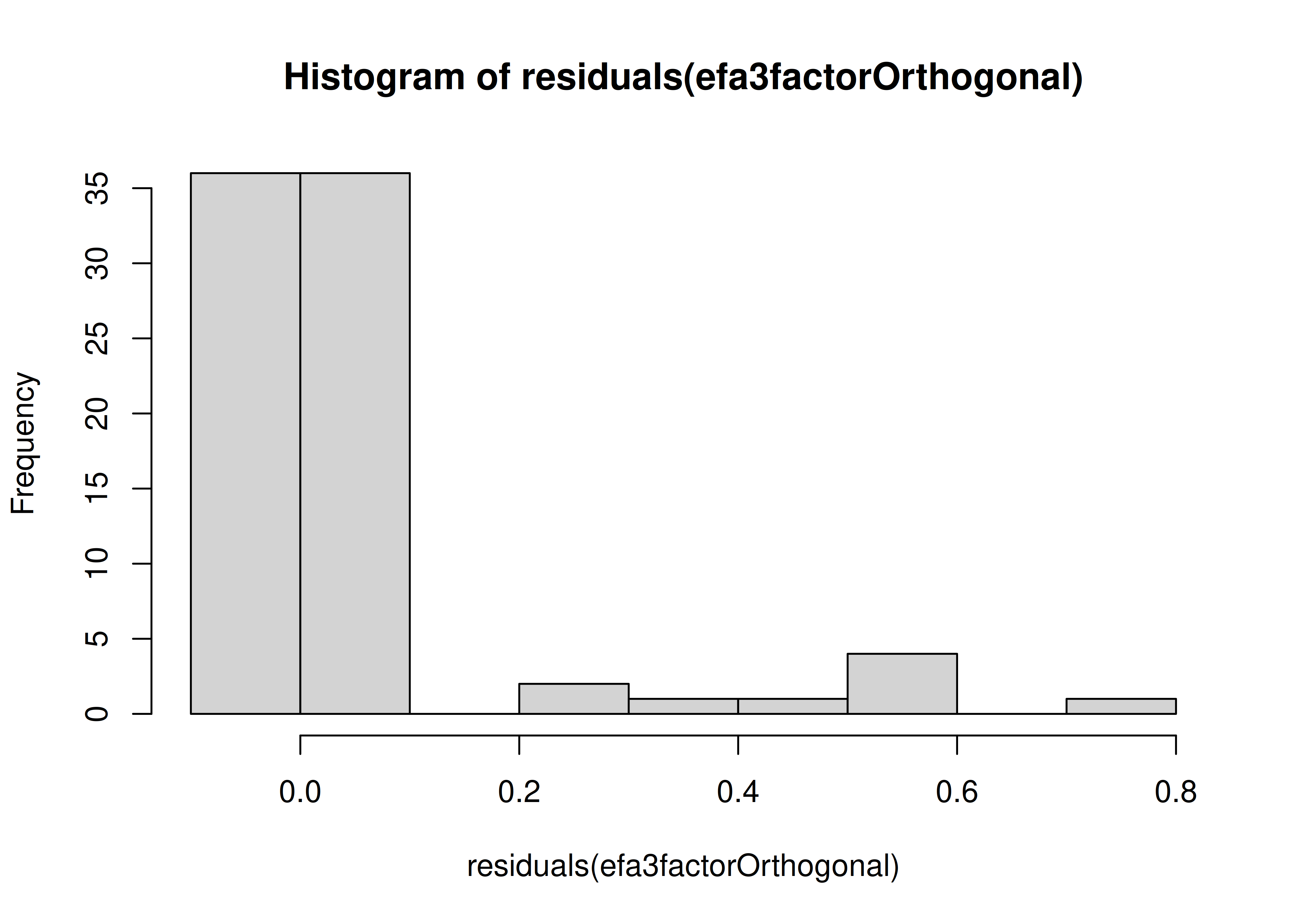
             x1            x2            x3            x4           x5
x1  0.525604637 -0.0121613494  0.0020909443  0.0481340574 -0.036771251
x2 -0.012161349  0.7448898000  0.0006576074 -0.0296115336  0.030848053
x3  0.002090944  0.0006576074  0.5019212070  0.0006260792 -0.015163678
x4  0.048134057 -0.0296115336  0.0006260792  0.2668740282 -0.001827322
x5 -0.036771251  0.0308480531 -0.0151636779 -0.0018273222  0.263188714
x6 -0.015033262  0.0001545610  0.0206794944 -0.0051858959  0.007660701
x7 -0.018931574 -0.0310098503  0.0281289383  0.0445961395 -0.035368460
x8  0.032636590  0.0241116342 -0.0347251123 -0.0359074265  0.016406036
x9 -0.017156197  0.0017870132  0.0158438483 -0.0168211784  0.036038114
             x6           x7           x8           x9
x1 -0.015033262 -0.018931574  0.032636590 -0.017156197
x2  0.000154561 -0.031009850  0.024111634  0.001787013
x3  0.020679494  0.028128938 -0.034725112  0.015843848
x4 -0.005185896  0.044596140 -0.035907426 -0.016821178
x5  0.007660701 -0.035368460  0.016406036  0.036038114
x6  0.360031487 -0.006967004  0.019779865 -0.024899374
x7 -0.006967004  0.505427999  0.002550111 -0.003589245
x8  0.019779865  0.002550111  0.460332518 -0.001611445
x9 -0.024899374 -0.003589245 -0.001611445  0.519163584
14.4.1.4.1.2 lavaan
Code
                      nfct=1  nfct=2  nfct=3  nfct=4  nfct=5
chisq                239.990 104.454  23.051   7.171   1.736
df                    27.000  19.000  12.000   6.000   1.000
pvalue                 0.000   0.000   0.027   0.305   0.188
chisq.scaled         235.316 112.999  23.723   5.251   0.365
df.scaled             27.000  19.000  12.000   6.000   1.000
pvalue.scaled          0.000   0.000   0.022   0.512   0.546
chisq.scaling.factor   1.020   0.924   0.972   1.366   4.755
baseline.chisq       693.305 693.305 693.305 693.305 693.305
baseline.df           36.000  36.000  36.000  36.000  36.000
baseline.pvalue        0.000   0.000   0.000   0.000   0.000
rmsea                  0.162   0.122   0.055   0.025   0.049
cfi                    0.676   0.870   0.983   0.998   0.999
tli                    0.568   0.754   0.950   0.989   0.960
srmr                   0.129   0.073   0.020   0.012   0.006
rmsea.robust           0.190   0.148   0.080   0.000   0.000
cfi.robust             0.664   0.865   0.988   1.000      NA
tli.robust 0.552 0.745 0.964 Inf NA$type
[1] "cor.bollen"
$cov
x1 x2 x3 x4 x5 x6 x7 x8 x9
x1 0.000
x2 -0.008 0.000
x3 0.001 -0.004 0.000
x4 0.040 -0.022 -0.001 0.000
x5 -0.019 0.013 -0.031 -0.004 0.000
x6 -0.034 0.015 0.024 -0.002 0.005 0.000
x7 -0.034 -0.037 0.027 0.035 -0.043 0.001 0.000
x8 0.027 0.029 -0.041 -0.044 0.016 0.016 -0.007 0.000
x9 -0.010 0.013 0.014 -0.033 0.042 -0.024 -0.009 -0.002 0.000
$mean
x1 x2 x3 x4 x5 x6 x7 x8 x9
0.003 -0.001 0.003 -0.003 -0.001 0.005 0.003 -0.001 0.003 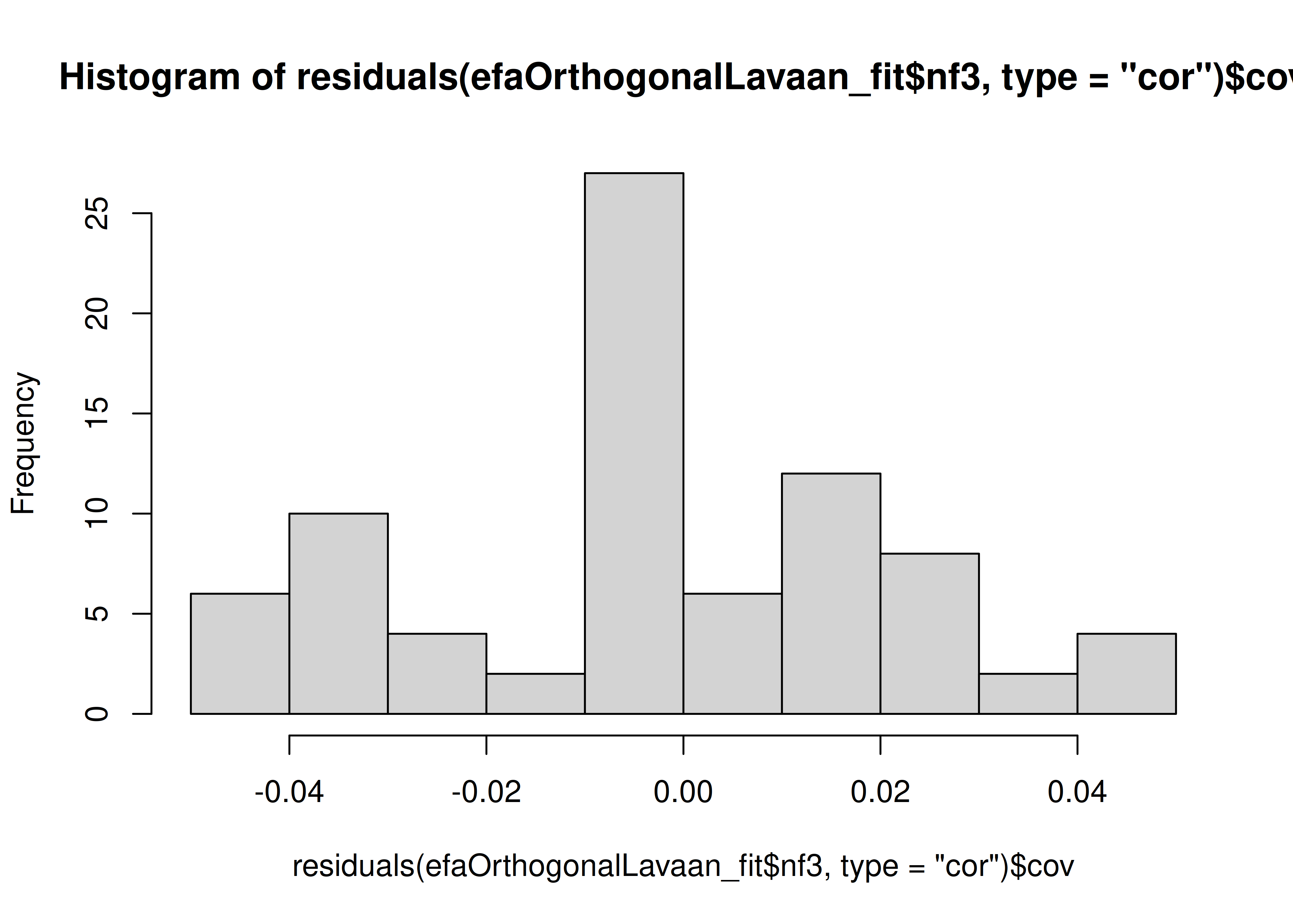
$type
[1] "cor.bollen"

$cov
       x1     x2     x3     x4     x5     x6     x7     x8     x9
x1  0.000
x2 -0.008  0.000
x3  0.001 -0.004  0.000
x4  0.040 -0.022 -0.001  0.000
x5 -0.019  0.013 -0.031 -0.004  0.000
x6 -0.034  0.015  0.024 -0.002  0.005  0.000
x7 -0.034 -0.037  0.027  0.035 -0.043  0.001  0.000
x8  0.027  0.029 -0.041 -0.044  0.016  0.016 -0.007  0.000
x9 -0.010  0.013  0.014 -0.033  0.042 -0.024 -0.009 -0.002  0.000

$mean
    x1     x2     x3     x4     x5     x6     x7     x8     x9
0.003 -0.001 0.003 -0.003 -0.001 0.005 0.003 -0.001 0.003 14.4.1.4.2 Oblique (Oblimin) rotation
14.4.1.4.2.1 psych
x1 x2 x3 x4 x5 x6 x7 x8 x9
x1 0.53
x2 -0.01 0.74
x3 0.00 0.00 0.50
x4 0.05 -0.03 0.00 0.27
x5 -0.04 0.03 -0.02 0.00 0.26
x6 -0.02 0.00 0.02 -0.01 0.01 0.36
x7 -0.02 -0.03 0.03 0.04 -0.04 -0.01 0.51
x8 0.03 0.02 -0.03 -0.04 0.02 0.02 0.00 0.46
x9 -0.02 0.00 0.02 -0.02 0.04 -0.02 0.00 0.00 0.52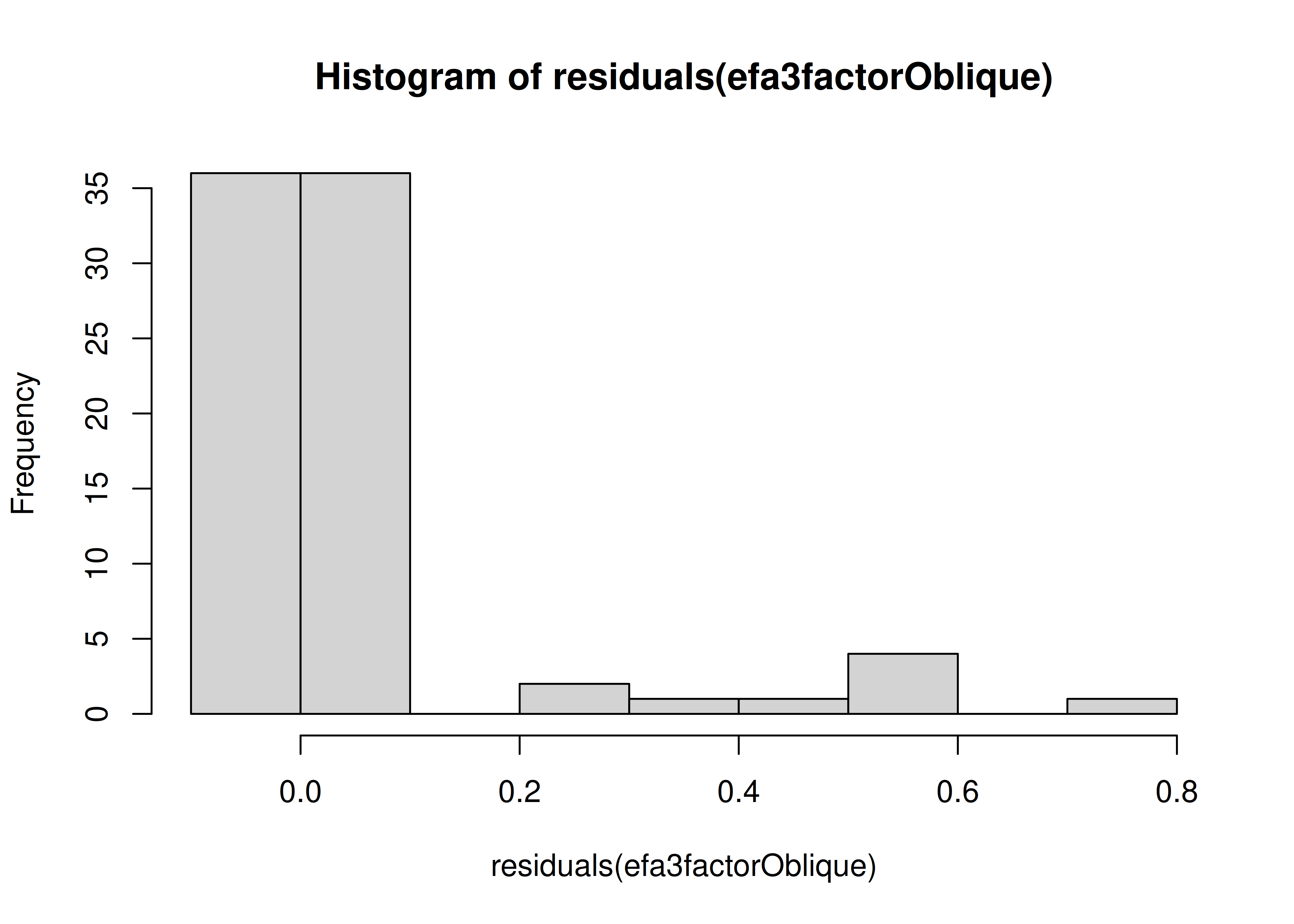
x1 x2 x3 x4 x5 x6
x1 0.609006606 0.005778083 0.04785250 0.224197219 0.149160462 0.151645536
x2 0.005778083 0.721805449 -0.01628447 0.094316026 0.164366228 0.116982126
x3 0.047852500 -0.016284471 0.48637804 0.219885172 0.215321248 0.226439421
x4 0.224197219 0.094316026 0.21988517 0.265514062 -0.001939637 -0.001399424
x5 0.149160462 0.164366228 0.21532125 -0.001939637 0.263236280 0.012613464
x6 0.151645536 0.116982126 0.22643942 -0.001399424 0.012613464 0.368286166
x7 0.129266226 0.087907675 0.17257093 0.141351101 0.052104575 0.084024198
x8 0.189010607 0.130179709 0.09641742 0.133399799 0.181072446 0.178880766
x9 0.111498418 0.068099418 0.10214055 0.191433127 0.246193720 0.170825288
x7 x8 x9
x1 0.129266226 0.189010607 0.11149842
x2 0.087907675 0.130179709 0.06809942
x3 0.172570930 0.096417423 0.10214055
x4 0.141351101 0.133399799 0.19143313
x5 0.052104575 0.181072446 0.24619372
x6 0.084024198 0.178880766 0.17082529
x7 0.448517388 0.001914572 0.06229779
x8 0.001914572 0.508094015 0.09255410
x9 0.062297795 0.092554098 0.6254431114.4.1.4.2.2 lavaan
Code
nfct=1 nfct=2 nfct=3 nfct=4 nfct=5
chisq 239.990 104.454 23.051 7.171 1.736
df 27.000 19.000 12.000 6.000 1.000
pvalue 0.000 0.000 0.027 0.305 0.188
chisq.scaled 235.316 112.999 23.723 5.251 0.365
df.scaled 27.000 19.000 12.000 6.000 1.000
pvalue.scaled 0.000 0.000 0.022 0.512 0.546
chisq.scaling.factor 1.020 0.924 0.972 1.366 4.755
baseline.chisq 693.305 693.305 693.305 693.305 693.305
baseline.df 36.000 36.000 36.000 36.000 36.000
baseline.pvalue 0.000 0.000 0.000 0.000 0.000
rmsea 0.162 0.122 0.055 0.025 0.049
cfi 0.676 0.870 0.983 0.998 0.999
tli 0.568 0.754 0.950 0.989 0.960
srmr 0.129 0.073 0.020 0.012 0.006
rmsea.robust 0.190 0.152 0.099 0.000 0.000
cfi.robust 0.664 0.868 1.000 NA NA
tli.robust 0.552 0.749 1.012 NA NA$type
[1] "cor.bollen"
$cov
x1 x2 x3 x4 x5 x6 x7 x8 x9
x1 0.000
x2 -0.008 0.000
x3 0.001 -0.004 0.000
x4 0.040 -0.022 -0.001 0.000
x5 -0.019 0.013 -0.031 -0.004 0.000
x6 -0.034 0.015 0.024 -0.002 0.005 0.000
x7 -0.034 -0.037 0.027 0.035 -0.043 0.001 0.000
x8 0.027 0.029 -0.041 -0.044 0.016 0.016 -0.007 0.000
x9 -0.010 0.013 0.014 -0.033 0.042 -0.024 -0.009 -0.002 0.000
$mean
x1 x2 x3 x4 x5 x6 x7 x8 x9
0.003 -0.001 0.003 -0.003 -0.001 0.005 0.003 -0.001 0.003 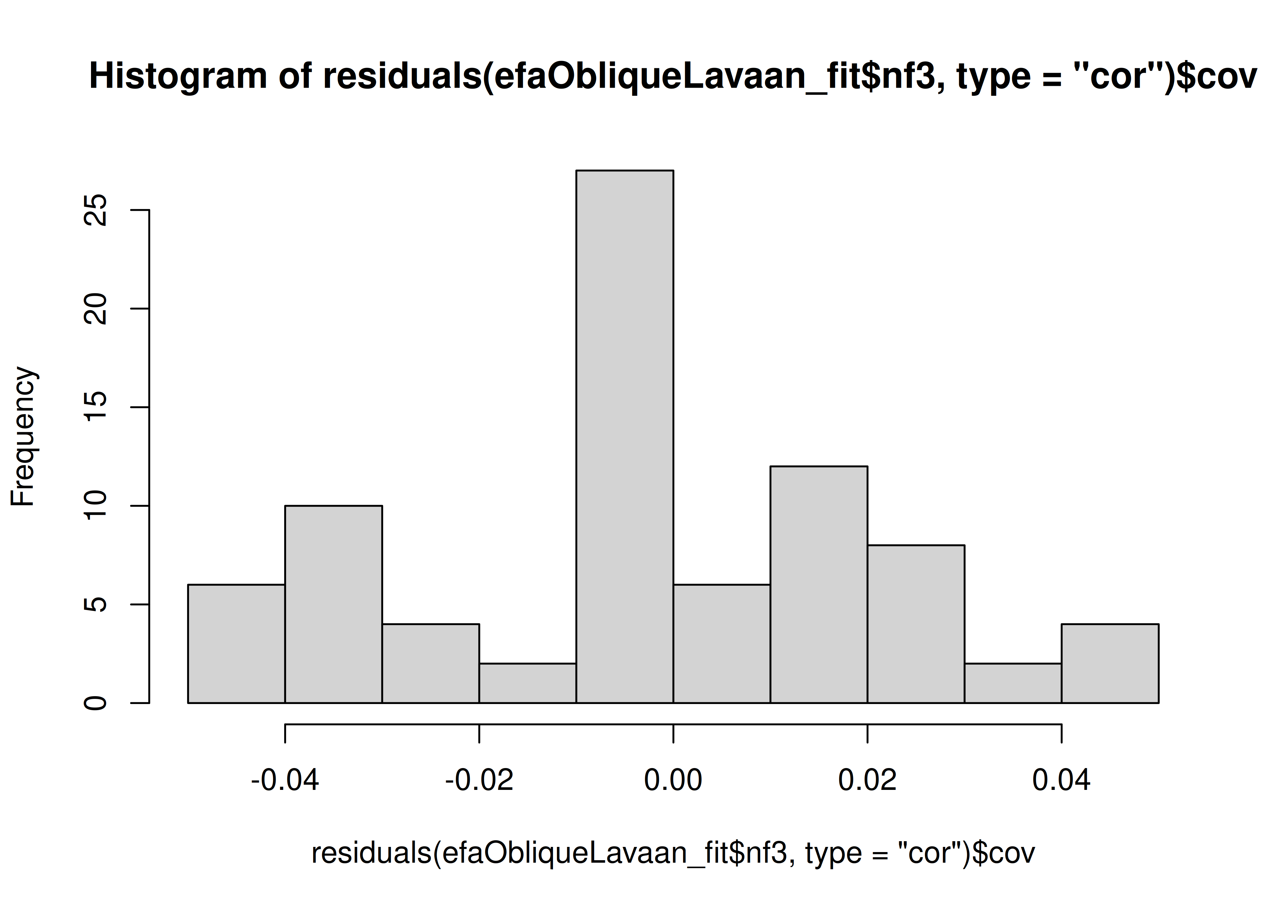
$type
[1] "cor.bollen"

$cov
       x1     x2     x3     x4     x5     x6     x7     x8     x9
x1  0.000
x2 -0.008  0.000
x3  0.001 -0.004  0.000
x4  0.040 -0.022 -0.001  0.000
x5 -0.019  0.013 -0.031 -0.004  0.000
x6 -0.034  0.015  0.024 -0.002  0.005  0.000
x7 -0.034 -0.037  0.027  0.035 -0.043  0.001  0.000
x8  0.027  0.029 -0.041 -0.044  0.016  0.016 -0.007  0.000
x9 -0.010  0.013  0.014 -0.033  0.042 -0.024 -0.009 -0.002  0.000

$mean
    x1     x2     x3     x4     x5     x6     x7     x8     x9
0.003 -0.001 0.003 -0.003 -0.001 0.005 0.003 -0.001 0.003 14.4.1.6 Plots
Biplots were generated using the psych package (Revelle, 2022).
Pairs panel plots were generated using the psych package (Revelle, 2022).
Correlation plots were generated using the corrplot package (Wei & Simko, 2021).
14.4.1.6.1 Orthogonal (Varimax) rotation
A scree plot from a model with orthogonal rotation is in Figure 14.36.
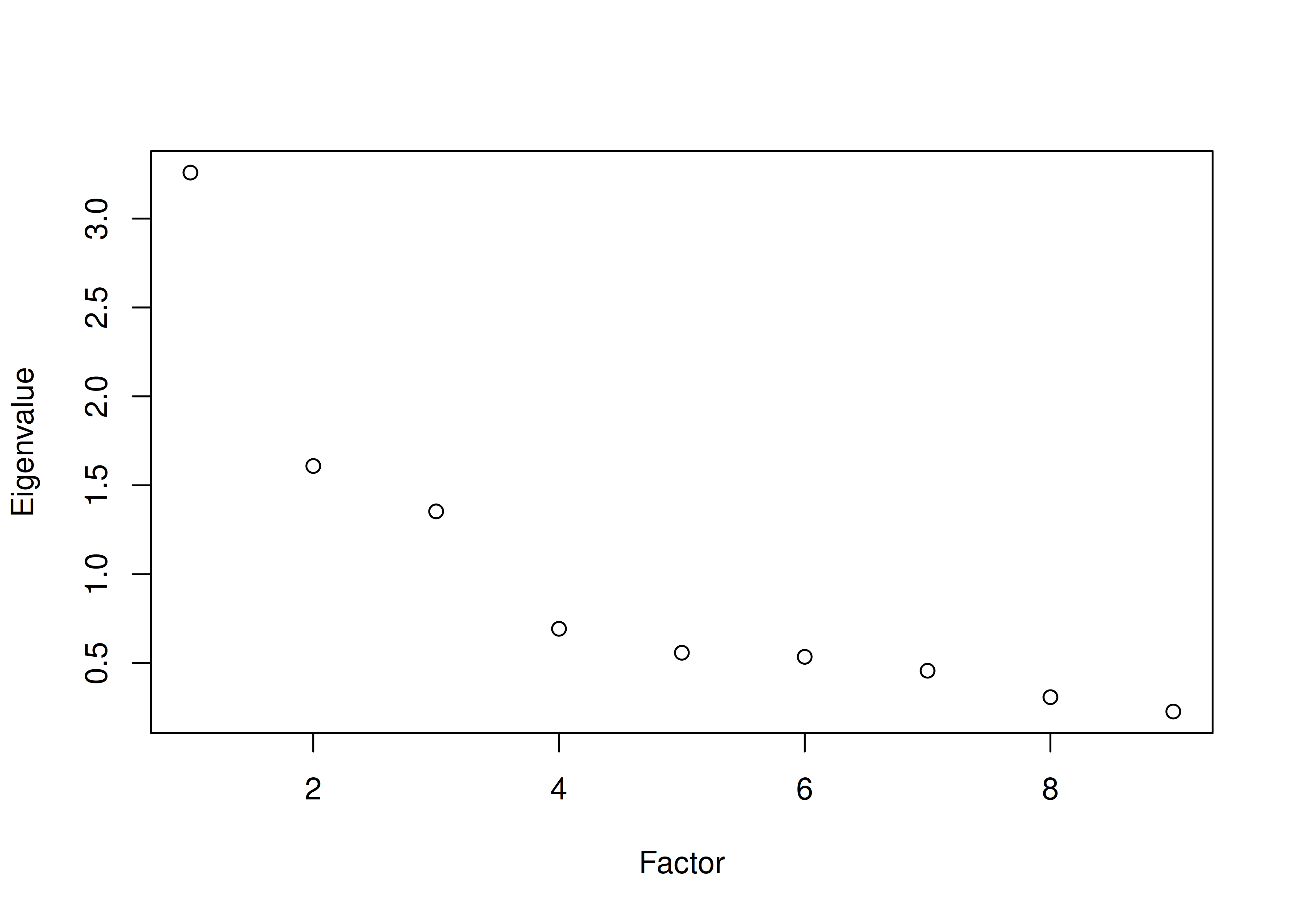
Figure 14.36: Scree Plot With Orthogonal Rotation in Exploratory Factor Analysis: psych.
A scree plot based on factor loadings from lavaan is in Figure 14.37.
When the factors are uncorrelated (orthogonal rotation), the eigenvalue for a factor is calculated as the sum of squared standardized factor loadings across all items, as described in Section 14.1.4.2.1.
Code
param1Factor <- parameterEstimates(
efa1factorOrthogonalLavaan_fit,
standardized = TRUE)
param2Factor <- parameterEstimates(
efa2factorOrthogonalLavaan_fit,
standardized = TRUE)
param3Factor <- parameterEstimates(
efa3factorOrthogonalLavaan_fit,
standardized = TRUE)
param4Factor <- parameterEstimates(
efa4factorOrthogonalLavaan_fit,
standardized = TRUE)
param5Factor <- parameterEstimates(
efa5factorOrthogonalLavaan_fit,
standardized = TRUE)
param6Factor <- parameterEstimates(
efa6factorOrthogonalLavaan_fit,
standardized = TRUE)
param7Factor <- parameterEstimates(
efa7factorOrthogonalLavaan_fit,
standardized = TRUE)
param8Factor <- parameterEstimates(
efa8factorOrthogonalLavaan_fit,
standardized = TRUE)
param9Factor <- parameterEstimates(
efa9factorOrthogonalLavaan_fit,
standardized = TRUE)
factorNames <- c("f1","f2","f3","f4","f5","f6","f7","f8","f9")
loadings1Factor <- param1Factor[which(
param1Factor$lhs %in% factorNames &
param1Factor$rhs %in% vars),
c("lhs","std.all")]
loadings2Factor <- param2Factor[which(
param2Factor$lhs %in% factorNames &
param2Factor$rhs %in% vars),
c("lhs","std.all")]
loadings3Factor <- param3Factor[which(
param3Factor$lhs %in% factorNames &
param3Factor$rhs %in% vars),
c("lhs","std.all")]
loadings4Factor <- param4Factor[which(
param4Factor$lhs %in% factorNames &
param4Factor$rhs %in% vars),
c("lhs","std.all")]
loadings5Factor <- param5Factor[which(
param5Factor$lhs %in% factorNames &
param5Factor$rhs %in% vars),
c("lhs","std.all")]
loadings6Factor <- param6Factor[which(
param6Factor$lhs %in% factorNames &
param6Factor$rhs %in% vars),
c("lhs","std.all")]
loadings7Factor <- param7Factor[which(
param7Factor$lhs %in% factorNames &
param7Factor$rhs %in% vars),
c("lhs","std.all")]
loadings8Factor <- param8Factor[which(
param8Factor$lhs %in% factorNames &
param8Factor$rhs %in% vars),
c("lhs","std.all")]
loadings9Factor <- param9Factor[which(
param9Factor$lhs %in% factorNames &
param9Factor$rhs %in% vars),
c("lhs","std.all")]
eigenData <- data.frame(
Factor = 1:9,
Eigenvalue = NA)
eigenData$Eigenvalue[which(
eigenData$Factor == 1)] <- sum(loadings1Factor$std.all^2)
eigenData$Eigenvalue[which(eigenData$Factor == 2)] <-
loadings2Factor %>%
group_by(lhs) %>%
summarise(
Eigenvalue = sum(std.all^2),
.groups = "drop") %>%
summarise(min(Eigenvalue))
eigenData$Eigenvalue[which(eigenData$Factor == 3)] <-
loadings3Factor %>%
group_by(lhs) %>%
summarise(
Eigenvalue = sum(std.all^2),
.groups = "drop") %>%
summarise(min(Eigenvalue))
eigenData$Eigenvalue[which(eigenData$Factor == 4)] <-
loadings4Factor %>%
group_by(lhs) %>%
summarise(
Eigenvalue = sum(std.all^2),
.groups = "drop") %>%
summarise(min(Eigenvalue))
eigenData$Eigenvalue[which(eigenData$Factor == 5)] <-
loadings5Factor %>%
group_by(lhs) %>%
summarise(
Eigenvalue = sum(std.all^2),
.groups = "drop") %>%
summarise(min(Eigenvalue))
eigenData$Eigenvalue[which(eigenData$Factor == 6)] <-
loadings6Factor %>%
group_by(lhs) %>%
summarise(
Eigenvalue = sum(std.all^2),
.groups = "drop") %>%
summarise(min(Eigenvalue))
eigenData$Eigenvalue[which(eigenData$Factor == 7)] <-
loadings7Factor %>%
group_by(lhs) %>%
summarise(
Eigenvalue = sum(std.all^2),
.groups = "drop") %>%
summarise(min(Eigenvalue))
eigenData$Eigenvalue[which(eigenData$Factor == 8)] <-
loadings8Factor %>%
group_by(lhs) %>%
summarise(
Eigenvalue = sum(std.all^2),
.groups = "drop") %>%
summarise(min(Eigenvalue))
eigenData$Eigenvalue[which(eigenData$Factor == 9)] <-
loadings9Factor %>%
group_by(lhs) %>%
summarise(
Eigenvalue = sum(std.all^2),
.groups = "drop") %>%
summarise(min(Eigenvalue))
plot(
eigenData$Factor,
eigenData$Eigenvalue,
xlab = "Factor",
ylab = "Eigevalue")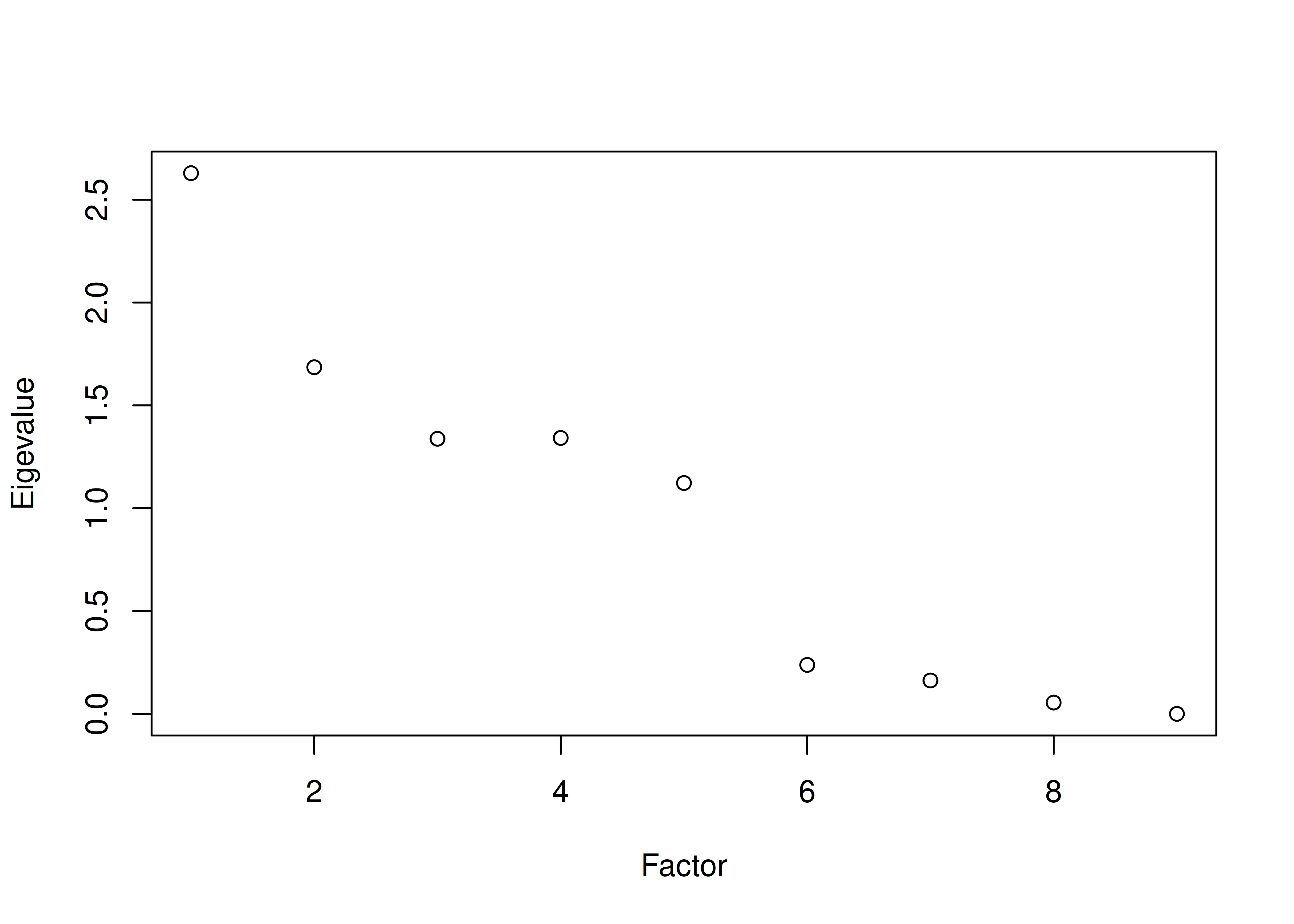
Figure 14.37: Scree Plot With Orthogonal Rotation in Exploratory Factor Analysis: lavaan.
A biplot is in Figure 14.38.
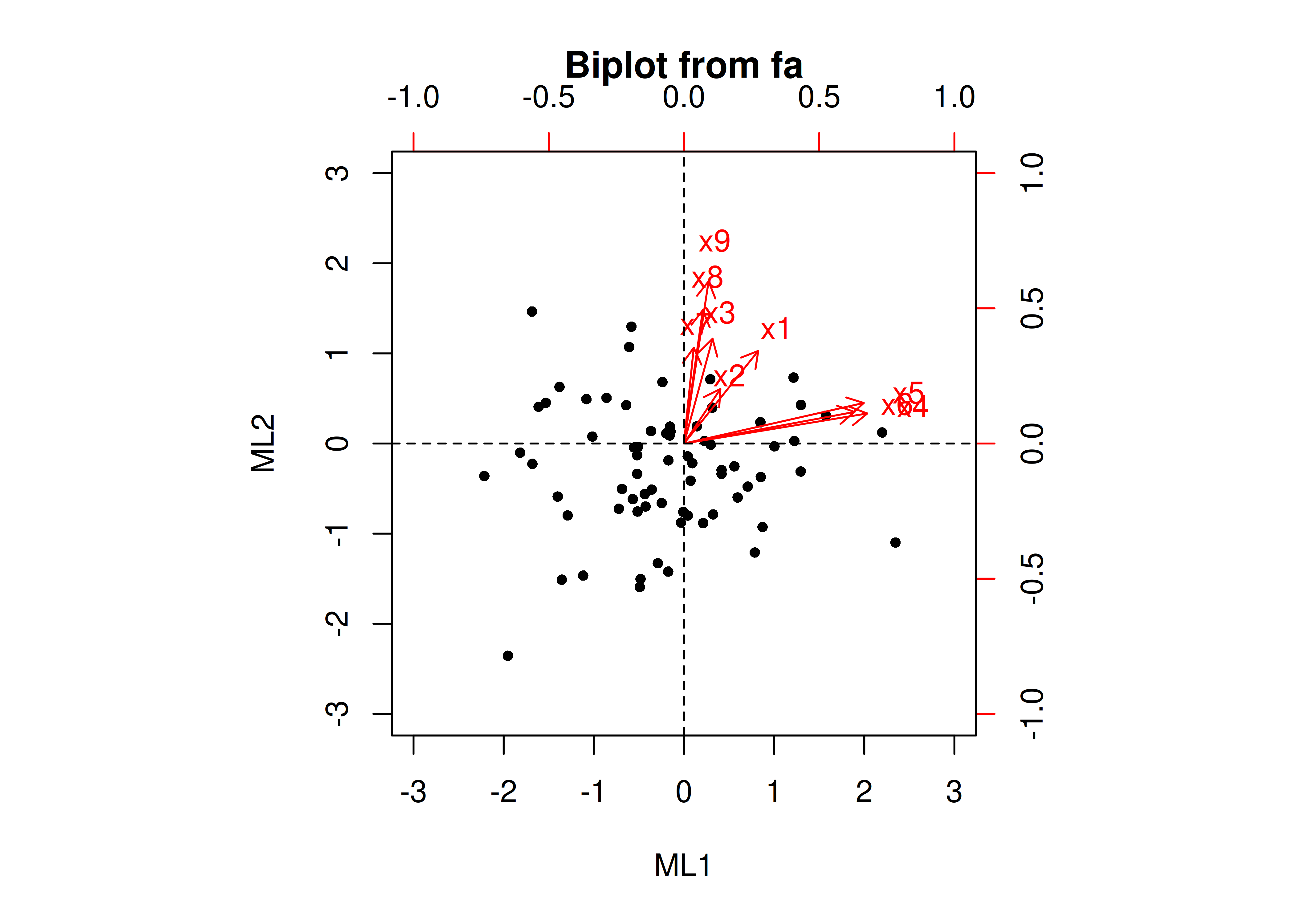
Figure 14.38: Biplot Using Orthogonal Rotation in Exploratory Factor Analysis.
A factor plot is in Figure 14.39.
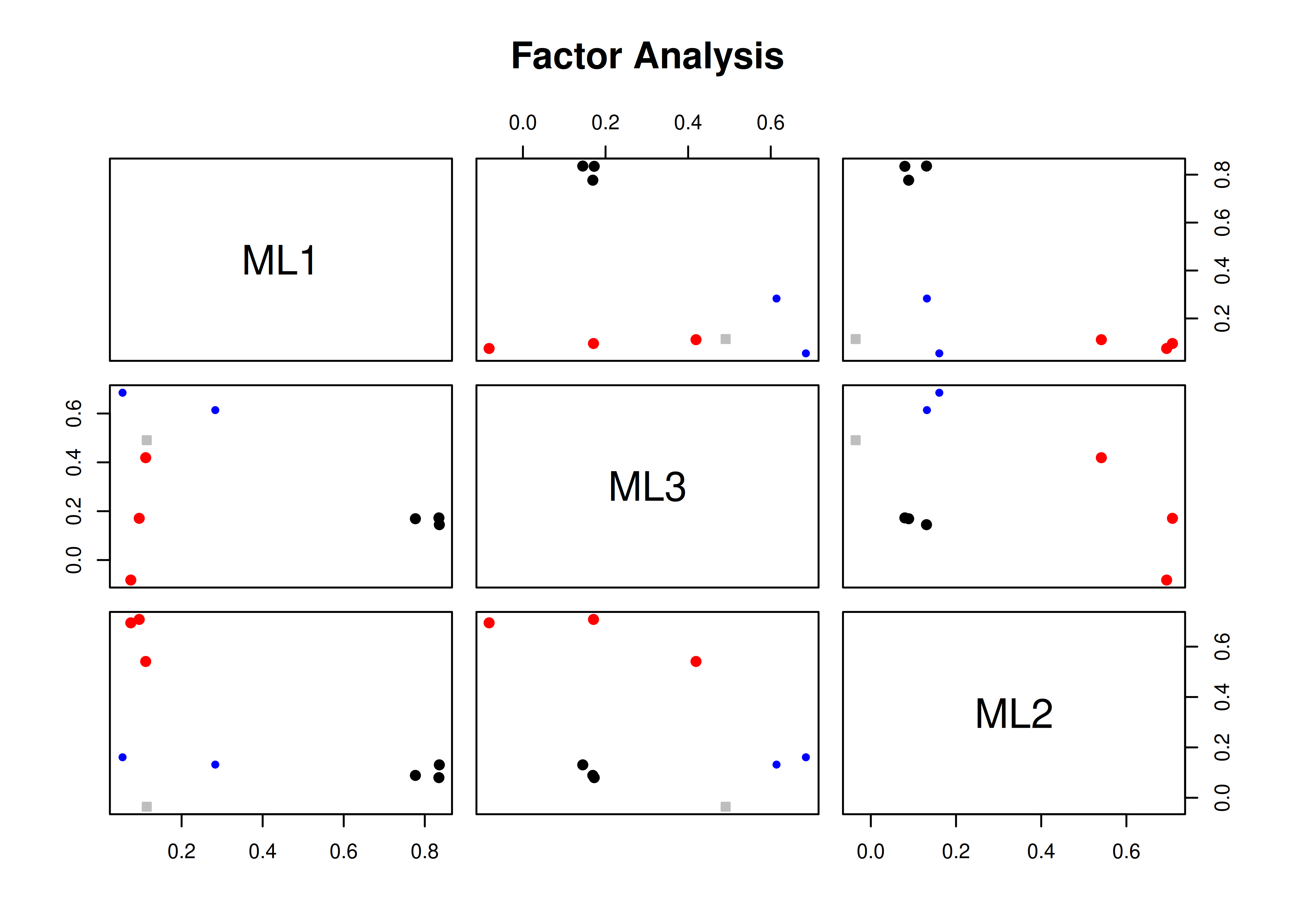
Figure 14.39: Factor Plot With Orthogonal Rotation in Exploratory Factor Analysis.
A factor diagram is in Figure 14.40.
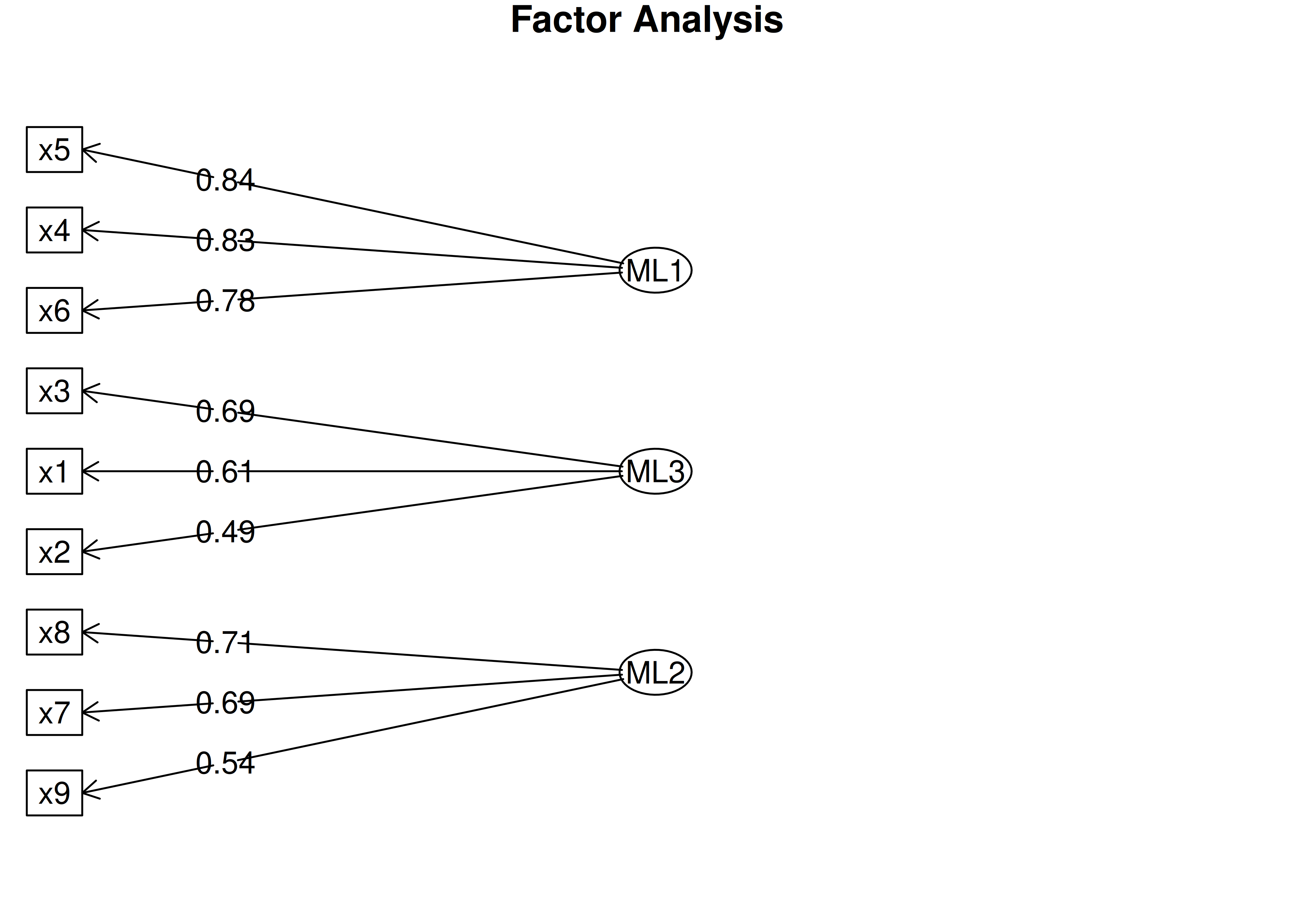
Figure 14.40: Factor Diagram With Orthogonal Rotation in Exploratory Factor Analysis.
A pairs panel plot is in Figure 14.41.
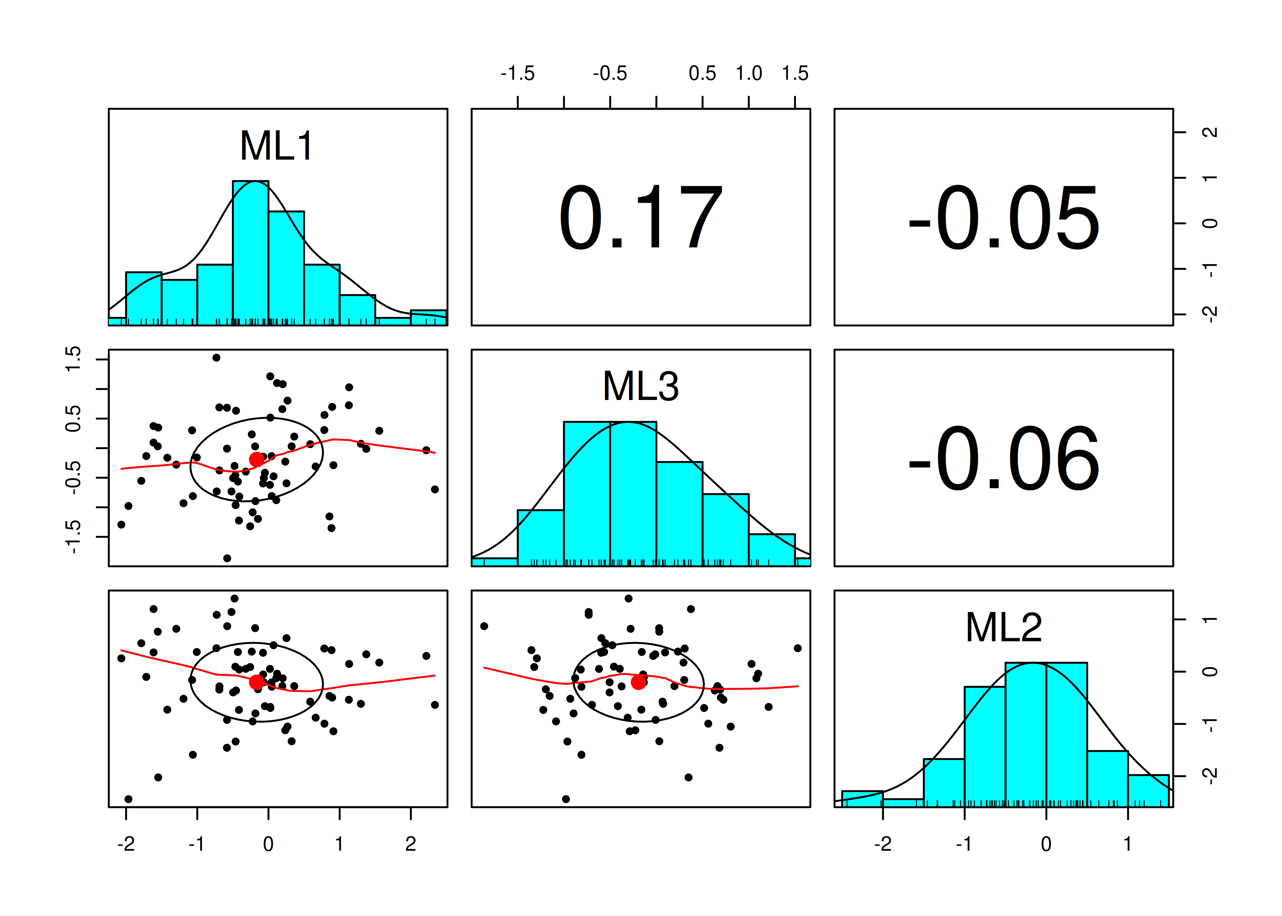
Figure 14.41: Pairs Panel Plot With Orthogonal Rotation in Exploratory Factor Analysis.
A correlation plot is in Figure 14.42.
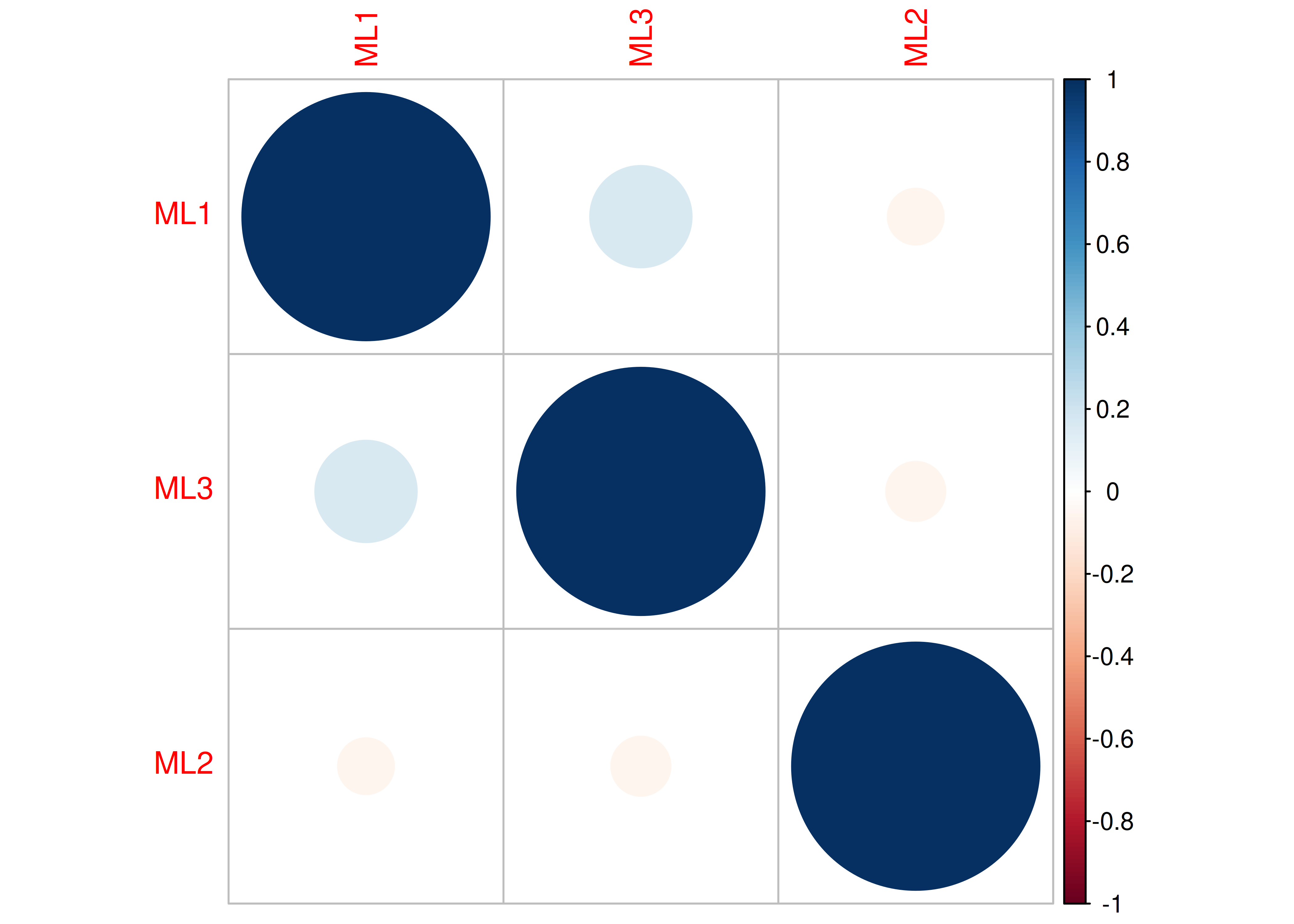
Figure 14.42: Correlation Plot With Orthogonal Rotation in Exploratory Factor Analysis.
14.4.1.6.2 Oblique (Oblimin) rotation
A biplot is in Figure 14.43.
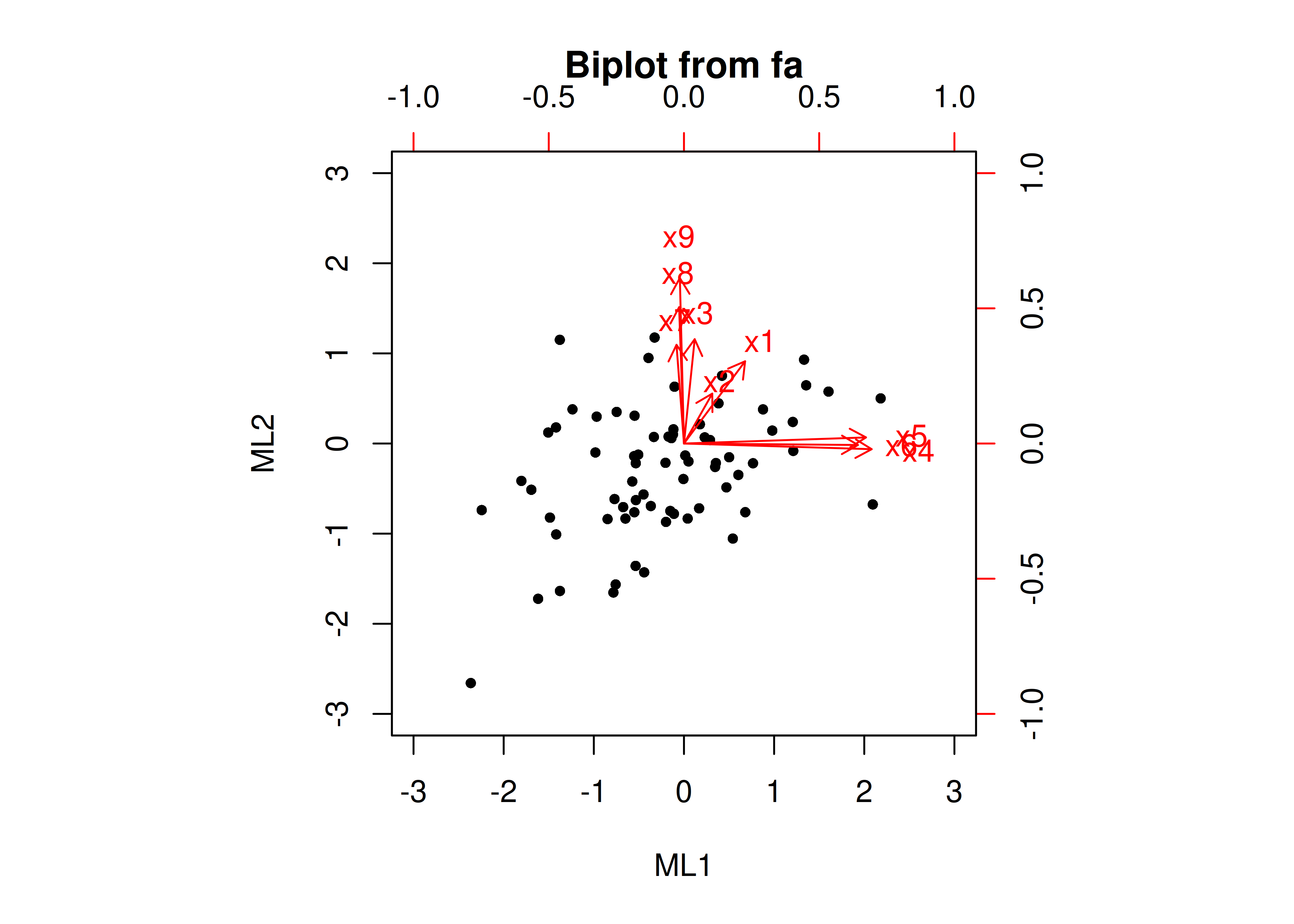
Figure 14.43: Biplot Using Oblique Rotation in Exploratory Factor Analysis.
A factor plot is in Figure 14.44.
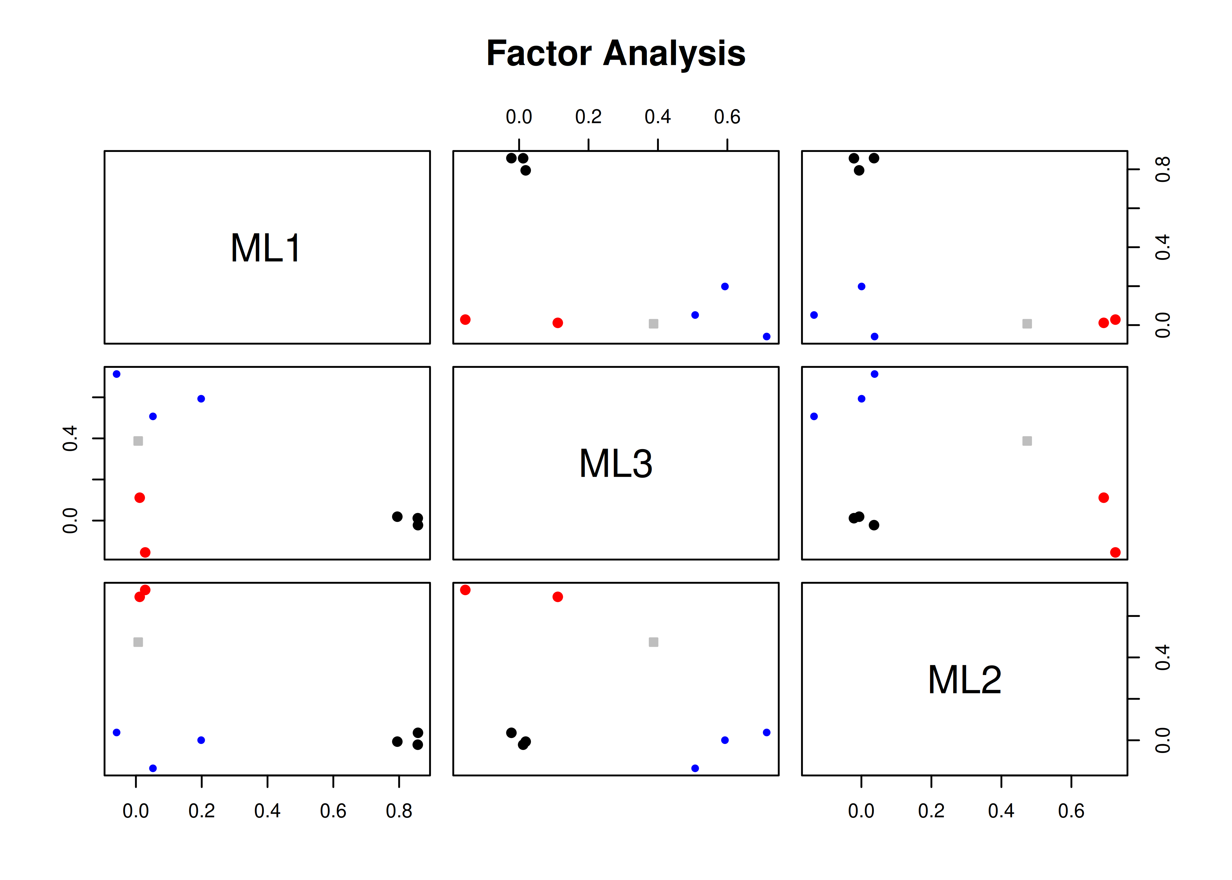
Figure 14.44: Factor Plot With Oblique Rotation in Exploratory Factor Analysis.
A factor diagram is in Figure 14.45.
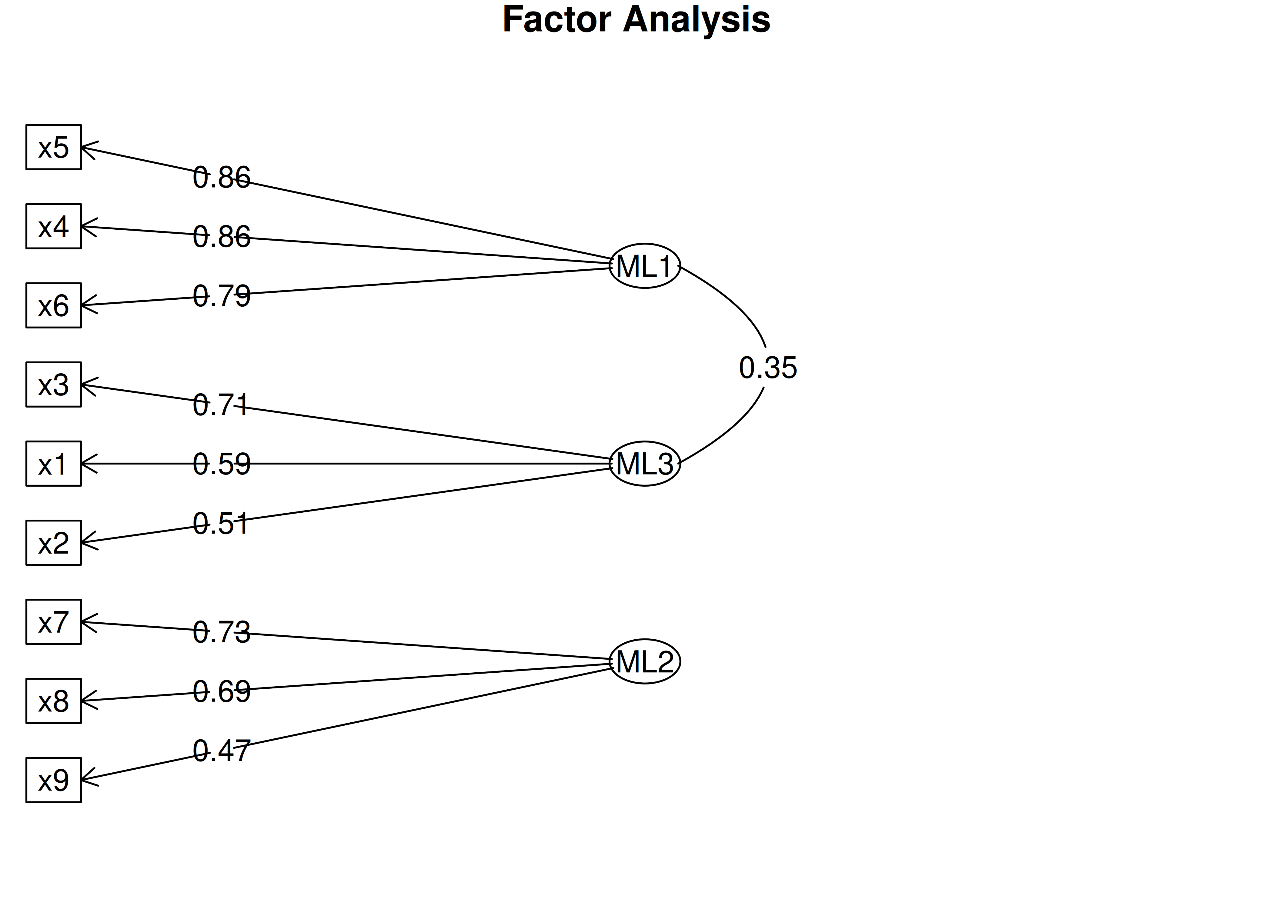
Figure 14.45: Factor Diagram With Oblique Rotation in Exploratory Factor Analysis.
A pairs panel plot is in Figure 14.46.
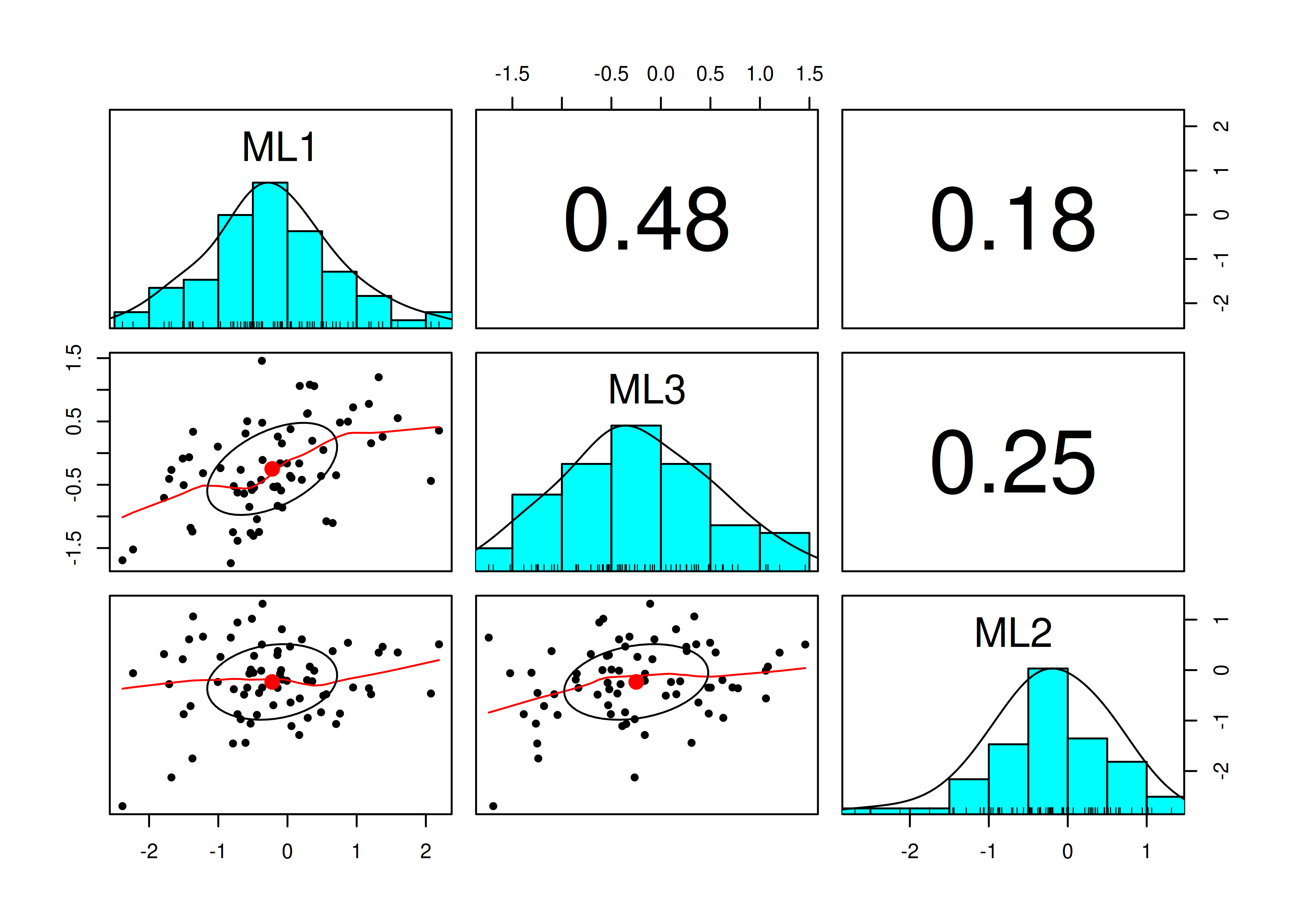
Figure 14.46: Pairs Panel Plot With Oblique Rotation in Exploratory Factor Analysis.
A correlation plot is in Figure 14.47.

Figure 14.47: Correlation Plot With Oblique Rotation in Exploratory Factor Analysis.
14.4.2 Confirmatory Factor Analysis (CFA)
I introduced confirmatory factor analysis (CFA) models in Section 7.3.3 in the chapter on structural equation models.
The confirmatory factor analysis (CFA) models were fit in the lavaan package (Rosseel et al., 2022).
The examples were adapted from the lavaan documentation: https://lavaan.ugent.be/tutorial/cfa.html (archived at https://perma.cc/GKY3-9YE4)
14.4.2.1 Specify the model
Code
cfaModel_syntax <- '
#Factor loadings
visual =~ x1 + x2 + x3
textual =~ x4 + x5 + x6
speed =~ x7 + x8 + x9
'
cfaModel_fullSyntax <- '
#Factor loadings (free the factor loading of the first indicator)
visual =~ NA*x1 + x2 + x3
textual =~ NA*x4 + x5 + x6
speed =~ NA*x7 + x8 + x9
#Fix latent means to zero
visual ~ 0
textual ~ 0
speed ~ 0
#Fix latent variances to one
visual ~~ 1*visual
textual ~~ 1*textual
speed ~~ 1*speed
#Estimate covariances among latent variables
visual ~~ textual
visual ~~ speed
textual ~~ speed
#Estimate residual variances of manifest variables
x1 ~~ x1
x2 ~~ x2
x3 ~~ x3
x4 ~~ x4
x5 ~~ x5
x6 ~~ x6
x7 ~~ x7
x8 ~~ x8
x9 ~~ x9
#Free intercepts of manifest variables
x1 ~ int1*1
x2 ~ int2*1
x3 ~ int3*1
x4 ~ int4*1
x5 ~ int5*1
x6 ~ int6*1
x7 ~ int7*1
x8 ~ int8*1
x9 ~ int9*1
'14.4.2.3 Display summary output
lavaan 0.6-20 ended normally after 40 iterations
Estimator ML
Optimization method NLMINB
Number of model parameters 30
Number of observations 301
Number of missing patterns 75
Model Test User Model:
Standard Scaled
Test Statistic 65.643 63.641
Degrees of freedom 24 24
P-value (Chi-square) 0.000 0.000
Scaling correction factor 1.031
Yuan-Bentler correction (Mplus variant)
Model Test Baseline Model:
Test statistic 693.305 646.574
Degrees of freedom 36 36
P-value 0.000 0.000
Scaling correction factor 1.072
User Model versus Baseline Model:
Comparative Fit Index (CFI) 0.937 0.935
Tucker-Lewis Index (TLI) 0.905 0.903
Robust Comparative Fit Index (CFI) 0.930
Robust Tucker-Lewis Index (TLI) 0.894
Loglikelihood and Information Criteria:
Loglikelihood user model (H0) -3213.600 -3213.600
Scaling correction factor 1.090
for the MLR correction
Loglikelihood unrestricted model (H1) -3180.778 -3180.778
Scaling correction factor 1.064
for the MLR correction
Akaike (AIC) 6487.199 6487.199
Bayesian (BIC) 6598.413 6598.413
Sample-size adjusted Bayesian (SABIC) 6503.270 6503.270
Root Mean Square Error of Approximation:
RMSEA 0.076 0.074
90 Percent confidence interval - lower 0.054 0.053
90 Percent confidence interval - upper 0.098 0.096
P-value H_0: RMSEA <= 0.050 0.026 0.034
P-value H_0: RMSEA >= 0.080 0.403 0.349
Robust RMSEA 0.092
90 Percent confidence interval - lower 0.064
90 Percent confidence interval - upper 0.120
P-value H_0: Robust RMSEA <= 0.050 0.008
P-value H_0: Robust RMSEA >= 0.080 0.780
Standardized Root Mean Square Residual:
SRMR 0.061 0.061
Parameter Estimates:
Standard errors Sandwich
Information bread Observed
Observed information based on Hessian
Latent Variables:
Estimate Std.Err z-value P(>|z|) Std.lv Std.all
visual =~
x1 0.885 0.108 8.183 0.000 0.885 0.762
x2 0.521 0.086 6.037 0.000 0.521 0.451
x3 0.712 0.088 8.065 0.000 0.712 0.632
textual =~
x4 0.989 0.067 14.690 0.000 0.989 0.842
x5 1.121 0.066 16.890 0.000 1.121 0.866
x6 0.849 0.065 12.991 0.000 0.849 0.818
speed =~
x7 0.596 0.084 7.092 0.000 0.596 0.557
x8 0.742 0.096 7.703 0.000 0.742 0.733
x9 0.686 0.099 6.939 0.000 0.686 0.673
Covariances:
Estimate Std.Err z-value P(>|z|) Std.lv Std.all
visual ~~
textual 0.430 0.080 5.386 0.000 0.430 0.430
speed 0.465 0.110 4.213 0.000 0.465 0.465
textual ~~
speed 0.314 0.084 3.746 0.000 0.314 0.314
Intercepts:
Estimate Std.Err z-value P(>|z|) Std.lv Std.all
.x1 4.977 0.071 69.850 0.000 4.977 4.289
.x2 6.050 0.070 85.953 0.000 6.050 5.235
.x3 2.227 0.069 32.218 0.000 2.227 1.976
.x4 3.097 0.071 43.828 0.000 3.097 2.634
.x5 4.344 0.077 56.058 0.000 4.344 3.355
.x6 2.187 0.064 34.391 0.000 2.187 2.108
.x7 4.180 0.065 64.446 0.000 4.180 3.904
.x8 5.517 0.062 89.668 0.000 5.517 5.451
.x9 5.405 0.063 86.063 0.000 5.405 5.298
Variances:
Estimate Std.Err z-value P(>|z|) Std.lv Std.all
.x1 0.564 0.169 3.345 0.001 0.564 0.419
.x2 1.064 0.119 8.935 0.000 1.064 0.797
.x3 0.763 0.118 6.454 0.000 0.763 0.601
.x4 0.403 0.063 6.363 0.000 0.403 0.292
.x5 0.420 0.074 5.664 0.000 0.420 0.251
.x6 0.356 0.056 6.415 0.000 0.356 0.331
.x7 0.790 0.093 8.512 0.000 0.790 0.690
.x8 0.474 0.128 3.693 0.000 0.474 0.463
.x9 0.570 0.122 4.660 0.000 0.570 0.548
visual 1.000 1.000 1.000
textual 1.000 1.000 1.000
speed 1.000 1.000 1.000
R-Square:
Estimate
x1 0.581
x2 0.203
x3 0.399
x4 0.708
x5 0.749
x6 0.669
x7 0.310
x8 0.537
x9 0.452lavaan 0.6-20 ended normally after 40 iterations
Estimator ML
Optimization method NLMINB
Number of model parameters 30
Number of observations 301
Number of missing patterns 75
Model Test User Model:
Standard Scaled
Test Statistic 65.643 63.641
Degrees of freedom 24 24
P-value (Chi-square) 0.000 0.000
Scaling correction factor 1.031
Yuan-Bentler correction (Mplus variant)
Model Test Baseline Model:
Test statistic 693.305 646.574
Degrees of freedom 36 36
P-value 0.000 0.000
Scaling correction factor 1.072
User Model versus Baseline Model:
Comparative Fit Index (CFI) 0.937 0.935
Tucker-Lewis Index (TLI) 0.905 0.903
Robust Comparative Fit Index (CFI) 0.930
Robust Tucker-Lewis Index (TLI) 0.894
Loglikelihood and Information Criteria:
Loglikelihood user model (H0) -3213.600 -3213.600
Scaling correction factor 1.090
for the MLR correction
Loglikelihood unrestricted model (H1) -3180.778 -3180.778
Scaling correction factor 1.064
for the MLR correction
Akaike (AIC) 6487.199 6487.199
Bayesian (BIC) 6598.413 6598.413
Sample-size adjusted Bayesian (SABIC) 6503.270 6503.270
Root Mean Square Error of Approximation:
RMSEA 0.076 0.074
90 Percent confidence interval - lower 0.054 0.053
90 Percent confidence interval - upper 0.098 0.096
P-value H_0: RMSEA <= 0.050 0.026 0.034
P-value H_0: RMSEA >= 0.080 0.403 0.349
Robust RMSEA 0.092
90 Percent confidence interval - lower 0.064
90 Percent confidence interval - upper 0.120
P-value H_0: Robust RMSEA <= 0.050 0.008
P-value H_0: Robust RMSEA >= 0.080 0.780
Standardized Root Mean Square Residual:
SRMR 0.061 0.061
Parameter Estimates:
Standard errors Sandwich
Information bread Observed
Observed information based on Hessian
Latent Variables:
Estimate Std.Err z-value P(>|z|) Std.lv Std.all
visual =~
x1 0.885 0.108 8.183 0.000 0.885 0.762
x2 0.521 0.086 6.037 0.000 0.521 0.451
x3 0.712 0.088 8.065 0.000 0.712 0.632
textual =~
x4 0.989 0.067 14.690 0.000 0.989 0.842
x5 1.121 0.066 16.890 0.000 1.121 0.866
x6 0.849 0.065 12.991 0.000 0.849 0.818
speed =~
x7 0.596 0.084 7.092 0.000 0.596 0.557
x8 0.742 0.096 7.703 0.000 0.742 0.733
x9 0.686 0.099 6.939 0.000 0.686 0.673
Covariances:
Estimate Std.Err z-value P(>|z|) Std.lv Std.all
visual ~~
textual 0.430 0.080 5.386 0.000 0.430 0.430
speed 0.465 0.110 4.213 0.000 0.465 0.465
textual ~~
speed 0.314 0.084 3.746 0.000 0.314 0.314
Intercepts:
Estimate Std.Err z-value P(>|z|) Std.lv Std.all
visual 0.000 0.000 0.000
textual 0.000 0.000 0.000
speed 0.000 0.000 0.000
.x1 (int1) 4.977 0.071 69.850 0.000 4.977 4.289
.x2 (int2) 6.050 0.070 85.953 0.000 6.050 5.235
.x3 (int3) 2.227 0.069 32.218 0.000 2.227 1.976
.x4 (int4) 3.097 0.071 43.828 0.000 3.097 2.634
.x5 (int5) 4.344 0.077 56.058 0.000 4.344 3.355
.x6 (int6) 2.187 0.064 34.391 0.000 2.187 2.108
.x7 (int7) 4.180 0.065 64.446 0.000 4.180 3.904
.x8 (int8) 5.517 0.062 89.668 0.000 5.517 5.451
.x9 (int9) 5.405 0.063 86.063 0.000 5.405 5.298
Variances:
Estimate Std.Err z-value P(>|z|) Std.lv Std.all
visual 1.000 1.000 1.000
textual 1.000 1.000 1.000
speed 1.000 1.000 1.000
.x1 0.564 0.169 3.345 0.001 0.564 0.419
.x2 1.064 0.119 8.935 0.000 1.064 0.797
.x3 0.763 0.118 6.454 0.000 0.763 0.601
.x4 0.403 0.063 6.363 0.000 0.403 0.292
.x5 0.420 0.074 5.664 0.000 0.420 0.251
.x6 0.356 0.056 6.415 0.000 0.356 0.331
.x7 0.790 0.093 8.512 0.000 0.790 0.690
.x8 0.474 0.128 3.693 0.000 0.474 0.463
.x9 0.570 0.122 4.660 0.000 0.570 0.548
R-Square:
Estimate
x1 0.581
x2 0.203
x3 0.399
x4 0.708
x5 0.749
x6 0.669
x7 0.310
x8 0.537
x9 0.45214.4.2.4 Estimates of model fit
Code
chisq df pvalue
65.643 24.000 0.000
chisq.scaled df.scaled pvalue.scaled
63.641 24.000 0.000
chisq.scaling.factor baseline.chisq baseline.df
1.031 693.305 36.000
baseline.pvalue rmsea cfi
0.000 0.076 0.937
tli srmr rmsea.robust
0.905 0.061 0.092
cfi.robust tli.robust
0.930 0.894 14.4.2.5 Residuals
$type
[1] "cor.bollen"
$cov
x1 x2 x3 x4 x5 x6 x7 x8 x9
x1 0.000
x2 -0.020 0.000
x3 -0.019 0.053 0.000
x4 0.077 -0.035 -0.083 0.000
x5 0.015 -0.006 -0.119 0.004 0.000
x6 0.044 0.038 -0.002 -0.005 0.002 0.000
x7 -0.178 -0.215 -0.073 0.005 -0.061 -0.032 0.000
x8 -0.017 -0.053 -0.013 -0.088 -0.018 -0.008 0.062 0.000
x9 0.103 0.067 0.192 0.003 0.084 0.043 -0.031 -0.044 0.000
$mean
x1 x2 x3 x4 x5 x6 x7 x8 x9
0.001 -0.003 -0.002 -0.004 -0.003 0.006 0.000 0.002 0.000 14.4.2.7 Factor scores
14.4.2.7.1 Compare CFA factor scores to EFA factor scores
As would be expected, the factor scores from the CFA model are highly correlated with the factor scores from the EFA model.
Pearson's product-moment correlation
data: cfaFactorScores[, "visual"] and fa3Orthogonal[, "ML3"]
t = 15.64, df = 69, p-value < 2.2e-16
alternative hypothesis: true correlation is not equal to 0
95 percent confidence interval:
0.8185187 0.9257296
sample estimates:
cor
0.8831693
Pearson's product-moment correlation
data: cfaFactorScores[, "textual"] and fa3Orthogonal[, "ML1"]
t = 49.444, df = 69, p-value < 2.2e-16
alternative hypothesis: true correlation is not equal to 0
95 percent confidence interval:
0.9778619 0.9913860
sample estimates:
cor
0.9861797
Pearson's product-moment correlation
data: cfaFactorScores[, "speed"] and fa3Orthogonal[, "ML2"]
t = 17.78, df = 69, p-value < 2.2e-16
alternative hypothesis: true correlation is not equal to 0
95 percent confidence interval:
0.8530018 0.9405081
sample estimates:
cor
0.9060032 14.4.2.8 Internal Consistency Reliability
Internal consistency reliability of items composing the latent factors, as quantified by omega (\(\omega\)) and average variance extracted (AVE), was estimated using the semTools package (Jorgensen et al., 2021).
Coefficient omega (\(\omega\)) is an example of composite reliability.
visual textual speed
0.652 0.878 0.695 visual textual speed
0.397 0.713 0.430 14.4.2.9 Path diagram
A path diagram of the model generated using the semPlot package (Epskamp, 2022) is in Figure 14.48.
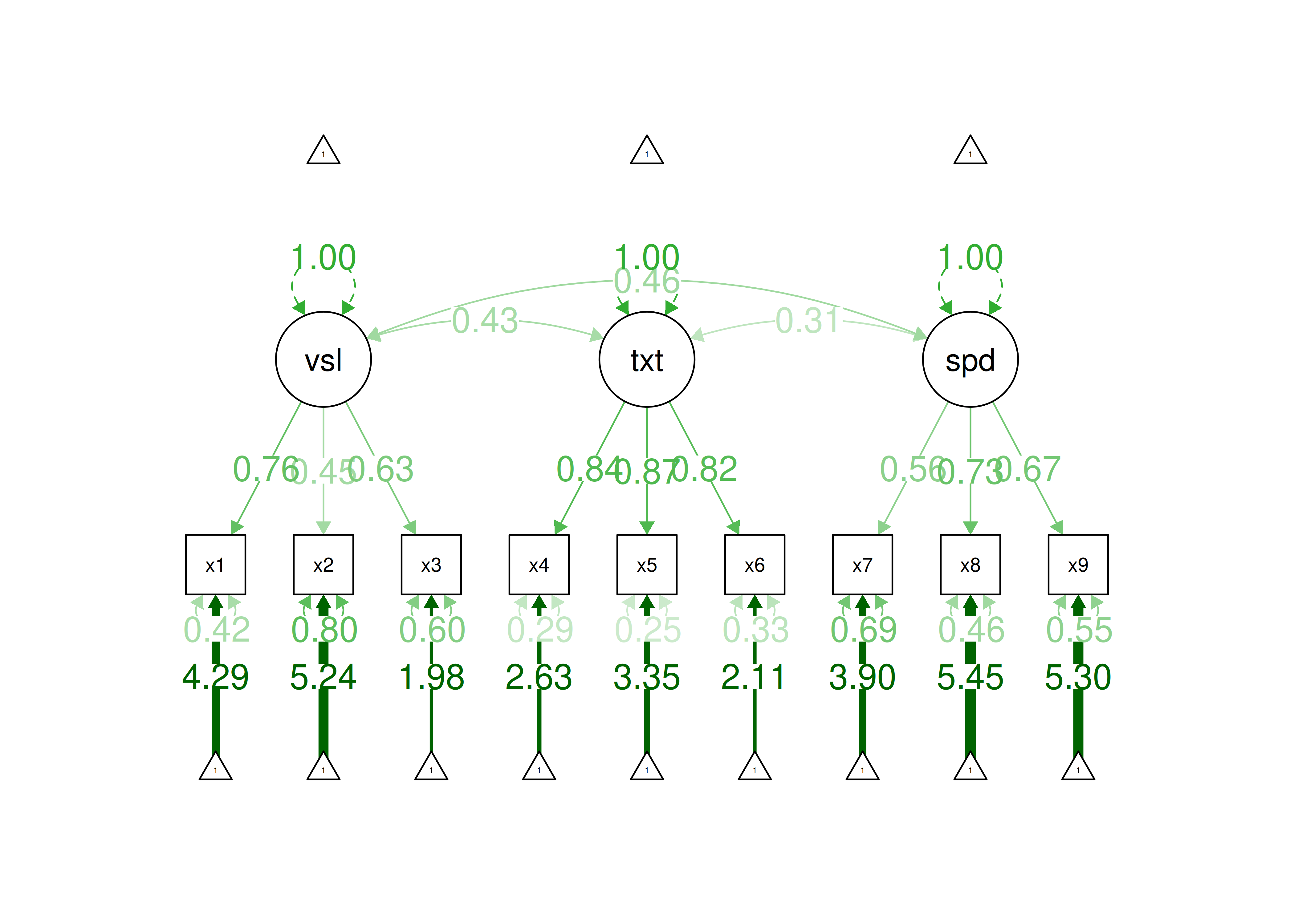
Figure 14.48: Confirmatory Factor Analysis Model Diagram.
14.4.2.10 Class Examples
14.4.2.10.1 Model 1
14.4.2.10.1.1 Create the covariance matrix
Code
correlationMatrixModel1 <- matrix(.6, nrow = 6, ncol = 6)
diag(correlationMatrixModel1) <- 1
rownames(correlationMatrixModel1) <- colnames(correlationMatrixModel1) <-
paste("V", 1:6, sep = "")
covarianceMatrixModel1 <- psych::cor2cov(
correlationMatrixModel1,
sigma = standardDeviations)
covarianceMatrixModel1 V1 V2 V3 V4 V5 V6
V1 1.0 0.6 0.6 0.6 0.6 0.6
V2 0.6 1.0 0.6 0.6 0.6 0.6
V3 0.6 0.6 1.0 0.6 0.6 0.6
V4 0.6 0.6 0.6 1.0 0.6 0.6
V5 0.6 0.6 0.6 0.6 1.0 0.6
V6 0.6 0.6 0.6 0.6 0.6 1.014.4.2.10.1.5 Display summary output
lavaan 0.6-20 ended normally after 10 iterations
Estimator ML
Optimization method NLMINB
Number of model parameters 12
Number of observations 300
Model Test User Model:
Test statistic 0.000
Degrees of freedom 9
P-value (Chi-square) 1.000
Model Test Baseline Model:
Test statistic 958.548
Degrees of freedom 15
P-value 0.000
User Model versus Baseline Model:
Comparative Fit Index (CFI) 1.000
Tucker-Lewis Index (TLI) 1.016
Loglikelihood and Information Criteria:
Loglikelihood user model (H0) -2071.810
Loglikelihood unrestricted model (H1) -2071.810
Akaike (AIC) 4167.621
Bayesian (BIC) 4212.066
Sample-size adjusted Bayesian (SABIC) 4174.009
Root Mean Square Error of Approximation:
RMSEA 0.000
90 Percent confidence interval - lower 0.000
90 Percent confidence interval - upper 0.000
P-value H_0: RMSEA <= 0.050 1.000
P-value H_0: RMSEA >= 0.080 0.000
Standardized Root Mean Square Residual:
SRMR 0.000
Parameter Estimates:
Standard errors Standard
Information Expected
Information saturated (h1) model Structured
Latent Variables:
Estimate Std.Err z-value P(>|z|) Std.lv Std.all
f1 =~
V1 0.773 0.050 15.390 0.000 0.773 0.775
V2 0.773 0.050 15.390 0.000 0.773 0.775
V3 0.773 0.050 15.390 0.000 0.773 0.775
V4 0.773 0.050 15.390 0.000 0.773 0.775
V5 0.773 0.050 15.390 0.000 0.773 0.775
V6 0.773 0.050 15.390 0.000 0.773 0.775
Variances:
Estimate Std.Err z-value P(>|z|) Std.lv Std.all
.V1 0.399 0.039 10.171 0.000 0.399 0.400
.V2 0.399 0.039 10.171 0.000 0.399 0.400
.V3 0.399 0.039 10.171 0.000 0.399 0.400
.V4 0.399 0.039 10.171 0.000 0.399 0.400
.V5 0.399 0.039 10.171 0.000 0.399 0.400
.V6 0.399 0.039 10.171 0.000 0.399 0.400
f1 1.000 1.000 1.000
R-Square:
Estimate
V1 0.600
V2 0.600
V3 0.600
V4 0.600
V5 0.600
V6 0.60014.4.2.10.1.6 Estimates of model fit
Code
chisq df pvalue rmsea cfi tli srmr
0.000 9.000 1.000 0.000 1.000 1.016 0.000 14.4.2.10.1.7 Residuals
$type
[1] "cor.bollen"
$cov
V1 V2 V3 V4 V5 V6
V1 0
V2 0 0
V3 0 0 0
V4 0 0 0 0
V5 0 0 0 0 0
V6 0 0 0 0 0 014.4.2.10.1.9 Internal Consistency Reliability
Internal consistency reliability of items composing the latent factors, as quantified by omega (\(\omega\)) and average variance extracted (AVE), was estimated using the semTools package (Jorgensen et al., 2021).
f1
0.9 f1
0.6 14.4.2.10.1.10 Path diagram
A path diagram of the model generated using the semPlot package (Epskamp, 2022) is in Figure 14.49.
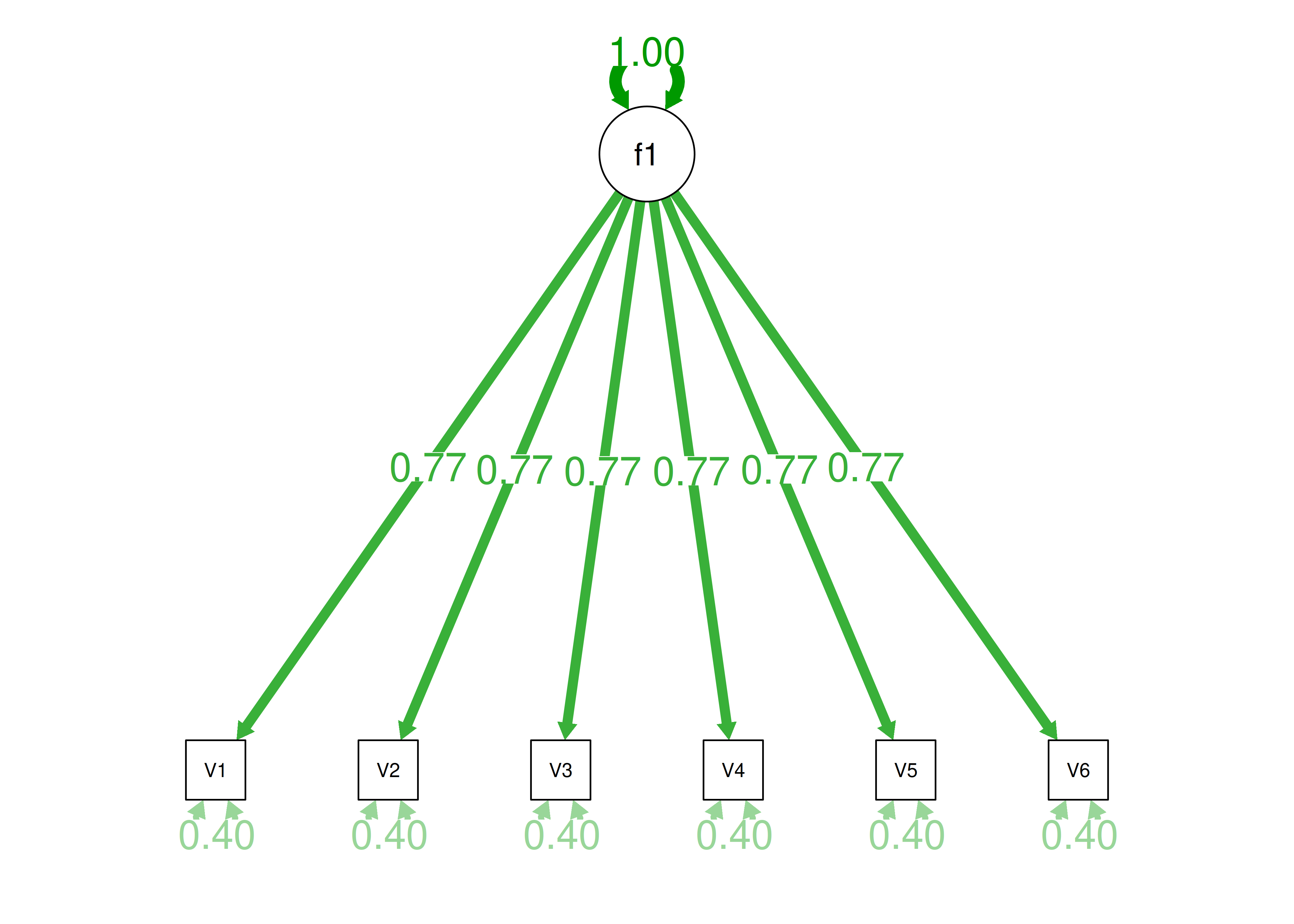
Figure 14.49: Confirmatory Factor Analysis Model 1 Diagram.
14.4.2.10.2 Model 2
14.4.2.10.2.1 Create the covariance matrix
Code
correlationMatrixModel2 <- matrix(0, nrow = 6, ncol = 6)
diag(correlationMatrixModel2) <- 1
rownames(correlationMatrixModel2) <- colnames(correlationMatrixModel2) <-
paste("V", 1:6, sep = "")
covarianceMatrixModel2 <- psych::cor2cov(
correlationMatrixModel2,
sigma = standardDeviations)
covarianceMatrixModel2 V1 V2 V3 V4 V5 V6
V1 1 0 0 0 0 0
V2 0 1 0 0 0 0
V3 0 0 1 0 0 0
V4 0 0 0 1 0 0
V5 0 0 0 0 1 0
V6 0 0 0 0 0 114.4.2.10.2.5 Display summary output
lavaan 0.6-20 ended normally after 23 iterations
Estimator ML
Optimization method NLMINB
Number of model parameters 12
Number of observations 300
Model Test User Model:
Test statistic 0.000
Degrees of freedom 9
P-value (Chi-square) 1.000
Model Test Baseline Model:
Test statistic 0.000
Degrees of freedom 15
P-value 1.000
User Model versus Baseline Model:
Comparative Fit Index (CFI) 1.000
Tucker-Lewis Index (TLI) 0.000
Loglikelihood and Information Criteria:
Loglikelihood user model (H0) -2551.084
Loglikelihood unrestricted model (H1) -2551.084
Akaike (AIC) 5126.169
Bayesian (BIC) 5170.614
Sample-size adjusted Bayesian (SABIC) 5132.557
Root Mean Square Error of Approximation:
RMSEA 0.000
90 Percent confidence interval - lower 0.000
90 Percent confidence interval - upper 0.000
P-value H_0: RMSEA <= 0.050 1.000
P-value H_0: RMSEA >= 0.080 0.000
Standardized Root Mean Square Residual:
SRMR 0.000
Parameter Estimates:
Standard errors Standard
Information Expected
Information saturated (h1) model Structured
Latent Variables:
Estimate Std.Err z-value P(>|z|) Std.lv Std.all
f1 =~
V1 0.000 227.294 0.000 1.000 0.000 0.000
V2 0.000 227.294 0.000 1.000 0.000 0.000
V3 0.000 227.294 0.000 1.000 0.000 0.000
V4 0.000 227.294 0.000 1.000 0.000 0.000
V5 0.000 227.294 0.000 1.000 0.000 0.000
V6 0.000 227.294 0.000 1.000 0.000 0.000
Variances:
Estimate Std.Err z-value P(>|z|) Std.lv Std.all
.V1 0.997 0.098 10.171 0.000 0.997 1.000
.V2 0.997 0.098 10.171 0.000 0.997 1.000
.V3 0.997 0.098 10.171 0.000 0.997 1.000
.V4 0.997 0.098 10.171 0.000 0.997 1.000
.V5 0.997 0.098 10.171 0.000 0.997 1.000
.V6 0.997 0.098 10.171 0.000 0.997 1.000
f1 1.000 1.000 1.000
R-Square:
Estimate
V1 0.000
V2 0.000
V3 0.000
V4 0.000
V5 0.000
V6 0.00014.4.2.10.2.7 Residuals
$type
[1] "cor.bollen"
$cov
V1 V2 V3 V4 V5 V6
V1 0
V2 0 0
V3 0 0 0
V4 0 0 0 0
V5 0 0 0 0 0
V6 0 0 0 0 0 014.4.2.10.2.9 Internal Consistency Reliability
Internal consistency reliability of items composing the latent factors, as quantified by omega (\(\omega\)) and average variance extracted (AVE), was estimated using the semTools package (Jorgensen et al., 2021).
f1
0 f1
0 14.4.2.10.2.10 Path diagram
A path diagram of the model generated using the semPlot package (Epskamp, 2022) is in Figure 14.50.
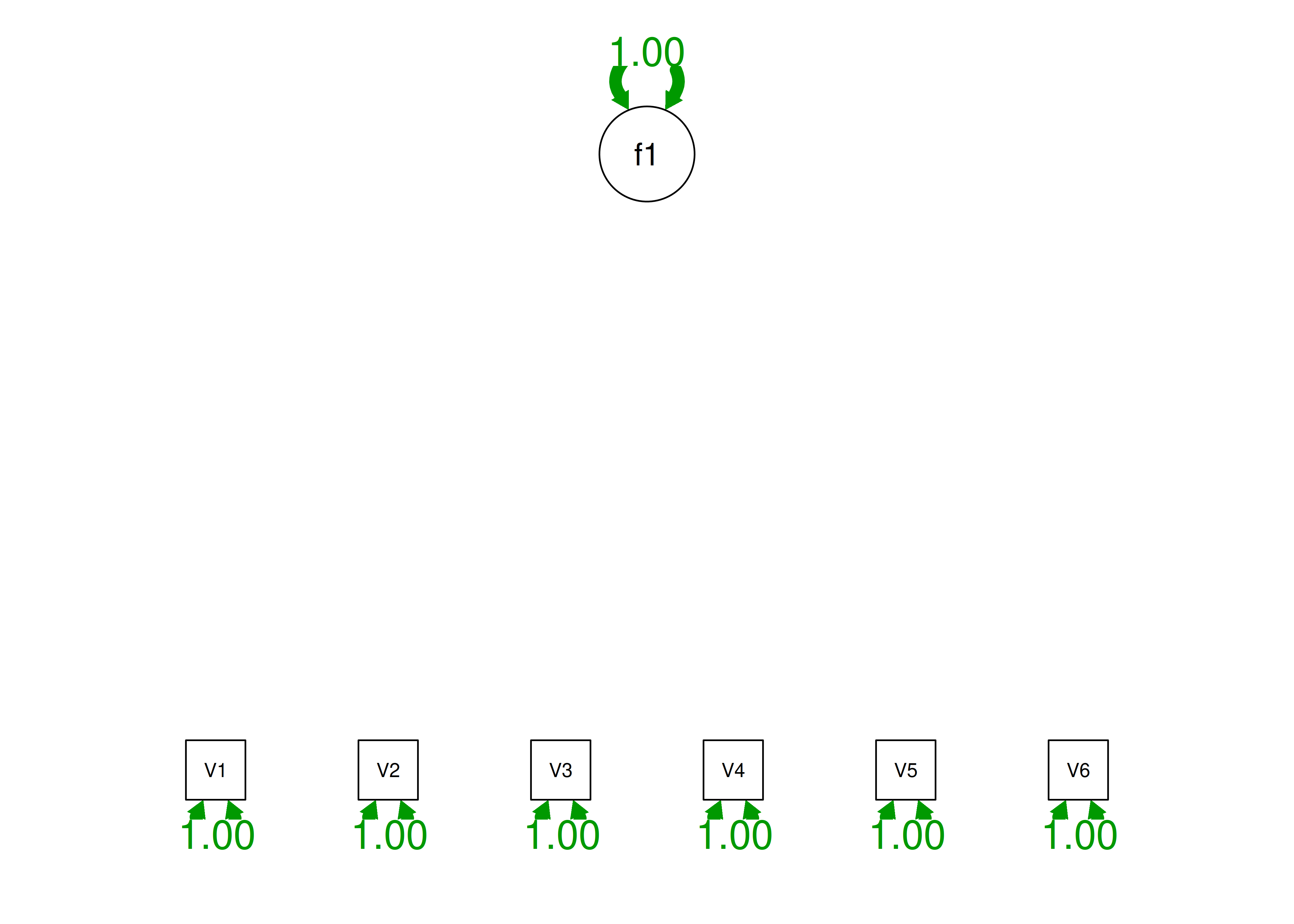
Figure 14.50: Confirmatory Factor Analysis Model 2 Diagram.
14.4.2.10.3 Model 3
14.4.2.10.3.1 Create the covariance matrix
Code
correlationMatrixModel3 <- matrix(c(
1,.6,.6,0,0,0,
.6,1,.6,0,0,0,
0,0,1,0,0,0,
0,0,0,1,.6,.6,
0,0,0,.6,1,.6,
0,0,0,.6,.6,1),
nrow = 6,
ncol = 6)
rownames(correlationMatrixModel3) <- colnames(correlationMatrixModel3) <-
paste("V", 1:6, sep = "")
covarianceMatrixModel3 <- psych::cor2cov(
correlationMatrixModel3,
sigma = standardDeviations)
covarianceMatrixModel3 V1 V2 V3 V4 V5 V6
V1 1.0 0.6 0 0.0 0.0 0.0
V2 0.6 1.0 0 0.0 0.0 0.0
V3 0.6 0.6 1 0.0 0.0 0.0
V4 0.0 0.0 0 1.0 0.6 0.6
V5 0.0 0.0 0 0.6 1.0 0.6
V6 0.0 0.0 0 0.6 0.6 1.014.4.2.10.3.5 Display summary output
lavaan 0.6-20 ended normally after 10 iterations
Estimator ML
Optimization method NLMINB
Number of model parameters 12
Number of observations 300
Model Test User Model:
Test statistic 313.237
Degrees of freedom 9
P-value (Chi-square) 0.000
Model Test Baseline Model:
Test statistic 626.474
Degrees of freedom 15
P-value 0.000
User Model versus Baseline Model:
Comparative Fit Index (CFI) 0.502
Tucker-Lewis Index (TLI) 0.171
Loglikelihood and Information Criteria:
Loglikelihood user model (H0) -2394.466
Loglikelihood unrestricted model (H1) -2237.847
Akaike (AIC) 4812.931
Bayesian (BIC) 4857.377
Sample-size adjusted Bayesian (SABIC) 4819.320
Root Mean Square Error of Approximation:
RMSEA 0.336
90 Percent confidence interval - lower 0.304
90 Percent confidence interval - upper 0.368
P-value H_0: RMSEA <= 0.050 0.000
P-value H_0: RMSEA >= 0.080 1.000
Standardized Root Mean Square Residual:
SRMR 0.227
Parameter Estimates:
Standard errors Standard
Information Expected
Information saturated (h1) model Structured
Latent Variables:
Estimate Std.Err z-value P(>|z|) Std.lv Std.all
f1 =~
V1 0.773 0.055 14.142 0.000 0.773 0.775
V2 0.773 0.055 14.142 0.000 0.773 0.775
V3 0.773 0.055 14.142 0.000 0.773 0.775
V4 0.000 0.064 0.000 1.000 0.000 0.000
V5 0.000 0.064 0.000 1.000 0.000 0.000
V6 0.000 0.064 0.000 1.000 0.000 0.000
Variances:
Estimate Std.Err z-value P(>|z|) Std.lv Std.all
.V1 0.399 0.051 7.746 0.000 0.399 0.400
.V2 0.399 0.051 7.746 0.000 0.399 0.400
.V3 0.399 0.051 7.746 0.000 0.399 0.400
.V4 0.997 0.081 12.247 0.000 0.997 1.000
.V5 0.997 0.081 12.247 0.000 0.997 1.000
.V6 0.997 0.081 12.247 0.000 0.997 1.000
f1 1.000 1.000 1.000
R-Square:
Estimate
V1 0.600
V2 0.600
V3 0.600
V4 0.000
V5 0.000
V6 0.000lavaan 0.6-20 ended normally after 8 iterations
Estimator ML
Optimization method NLMINB
Number of model parameters 13
Number of observations 300
Model Test User Model:
Test statistic 0.000
Degrees of freedom 8
P-value (Chi-square) 1.000
Model Test Baseline Model:
Test statistic 626.474
Degrees of freedom 15
P-value 0.000
User Model versus Baseline Model:
Comparative Fit Index (CFI) 1.000
Tucker-Lewis Index (TLI) 1.025
Loglikelihood and Information Criteria:
Loglikelihood user model (H0) -2237.847
Loglikelihood unrestricted model (H1) -2237.847
Akaike (AIC) 4501.694
Bayesian (BIC) 4549.843
Sample-size adjusted Bayesian (SABIC) 4508.615
Root Mean Square Error of Approximation:
RMSEA 0.000
90 Percent confidence interval - lower 0.000
90 Percent confidence interval - upper 0.000
P-value H_0: RMSEA <= 0.050 1.000
P-value H_0: RMSEA >= 0.080 0.000
Standardized Root Mean Square Residual:
SRMR 0.000
Parameter Estimates:
Standard errors Standard
Information Expected
Information saturated (h1) model Structured
Latent Variables:
Estimate Std.Err z-value P(>|z|) Std.lv Std.all
f1 =~
V1 0.773 0.055 14.142 0.000 0.773 0.775
V2 0.773 0.055 14.142 0.000 0.773 0.775
V3 0.773 0.055 14.142 0.000 0.773 0.775
f2 =~
V4 0.773 0.055 14.142 0.000 0.773 0.775
V5 0.773 0.055 14.142 0.000 0.773 0.775
V6 0.773 0.055 14.142 0.000 0.773 0.775
Covariances:
Estimate Std.Err z-value P(>|z|) Std.lv Std.all
f1 ~~
f2 0.000 0.071 0.000 1.000 0.000 0.000
Variances:
Estimate Std.Err z-value P(>|z|) Std.lv Std.all
.V1 0.399 0.051 7.746 0.000 0.399 0.400
.V2 0.399 0.051 7.746 0.000 0.399 0.400
.V3 0.399 0.051 7.746 0.000 0.399 0.400
.V4 0.399 0.051 7.746 0.000 0.399 0.400
.V5 0.399 0.051 7.746 0.000 0.399 0.400
.V6 0.399 0.051 7.746 0.000 0.399 0.400
f1 1.000 1.000 1.000
f2 1.000 1.000 1.000
R-Square:
Estimate
V1 0.600
V2 0.600
V3 0.600
V4 0.600
V5 0.600
V6 0.60014.4.2.10.3.6 Estimates of model fit
Code
chisq df pvalue rmsea cfi tli srmr
313.237 9.000 0.000 0.336 0.502 0.171 0.227 Code
chisq df pvalue rmsea cfi tli srmr
0.000 8.000 1.000 0.000 1.000 1.025 0.000 14.4.2.10.3.7 Compare model fit
Below is a test of whether the two-factor model fits better than the one-factor model. A significant chi-square difference test indicates that the two-factor model fits significantly better than the one-factor model.
14.4.2.10.3.8 Residuals
$type
[1] "cor.bollen"
$cov
V1 V2 V3 V4 V5 V6
V1 0.0
V2 0.0 0.0
V3 0.0 0.0 0.0
V4 0.0 0.0 0.0 0.0
V5 0.0 0.0 0.0 0.6 0.0
V6 0.0 0.0 0.0 0.6 0.6 0.0$type
[1] "cor.bollen"
$cov
V1 V2 V3 V4 V5 V6
V1 0
V2 0 0
V3 0 0 0
V4 0 0 0 0
V5 0 0 0 0 0
V6 0 0 0 0 0 014.4.2.10.3.10 Internal Consistency Reliability
Internal consistency reliability of items composing the latent factors, as quantified by omega (\(\omega\)) and average variance extracted (AVE), was estimated using the semTools package (Jorgensen et al., 2021).
f1
0.818 f1 f2
0.818 0.818 f1
0.6 f1 f2
0.6 0.6 14.4.2.10.3.11 Path diagram
Path diagrams of the models generated using the semPlot package (Epskamp, 2022) are in Figures 14.51 and 14.52.
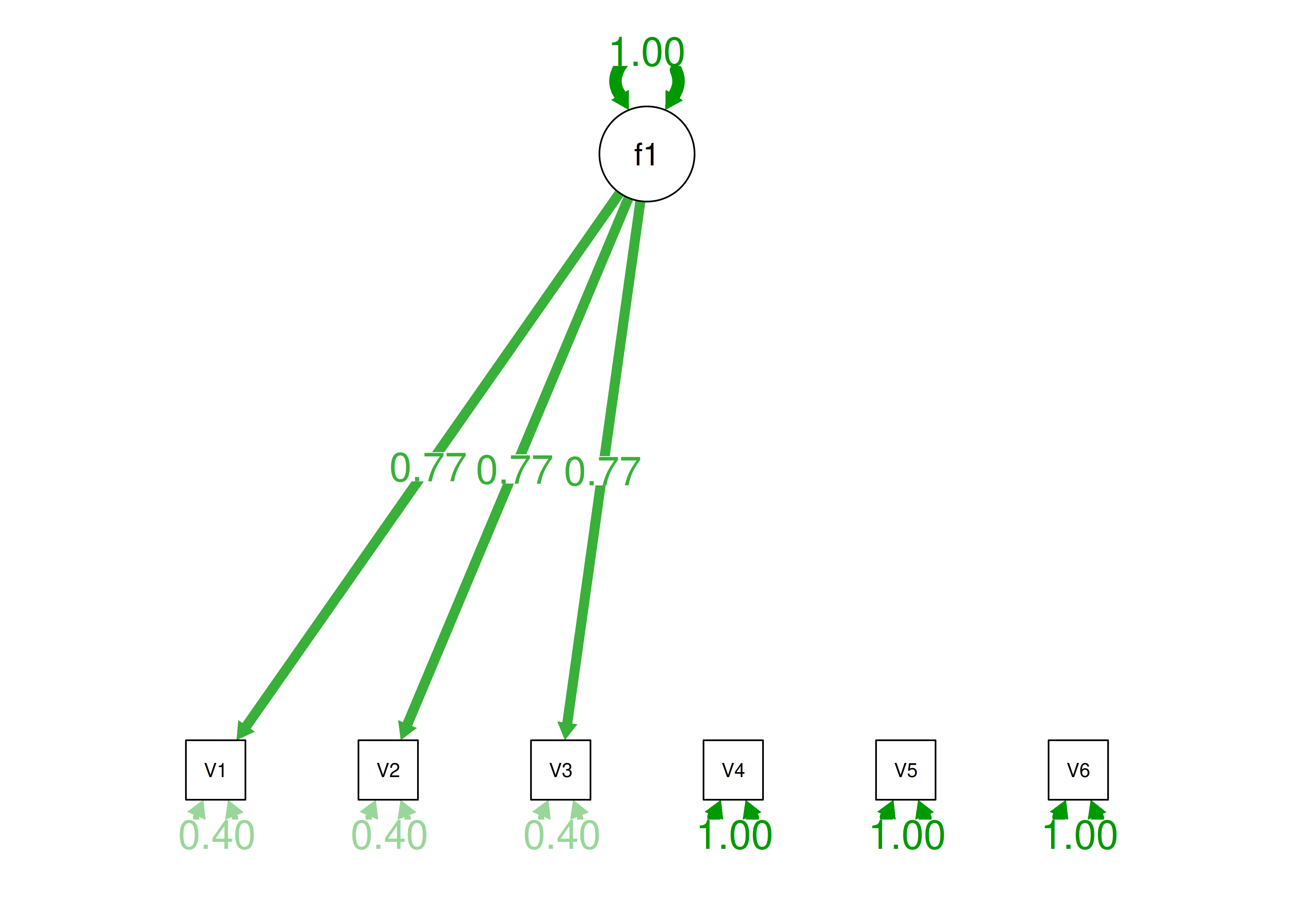
Figure 14.51: Confirmatory Factor Analysis Model 3a Diagram.
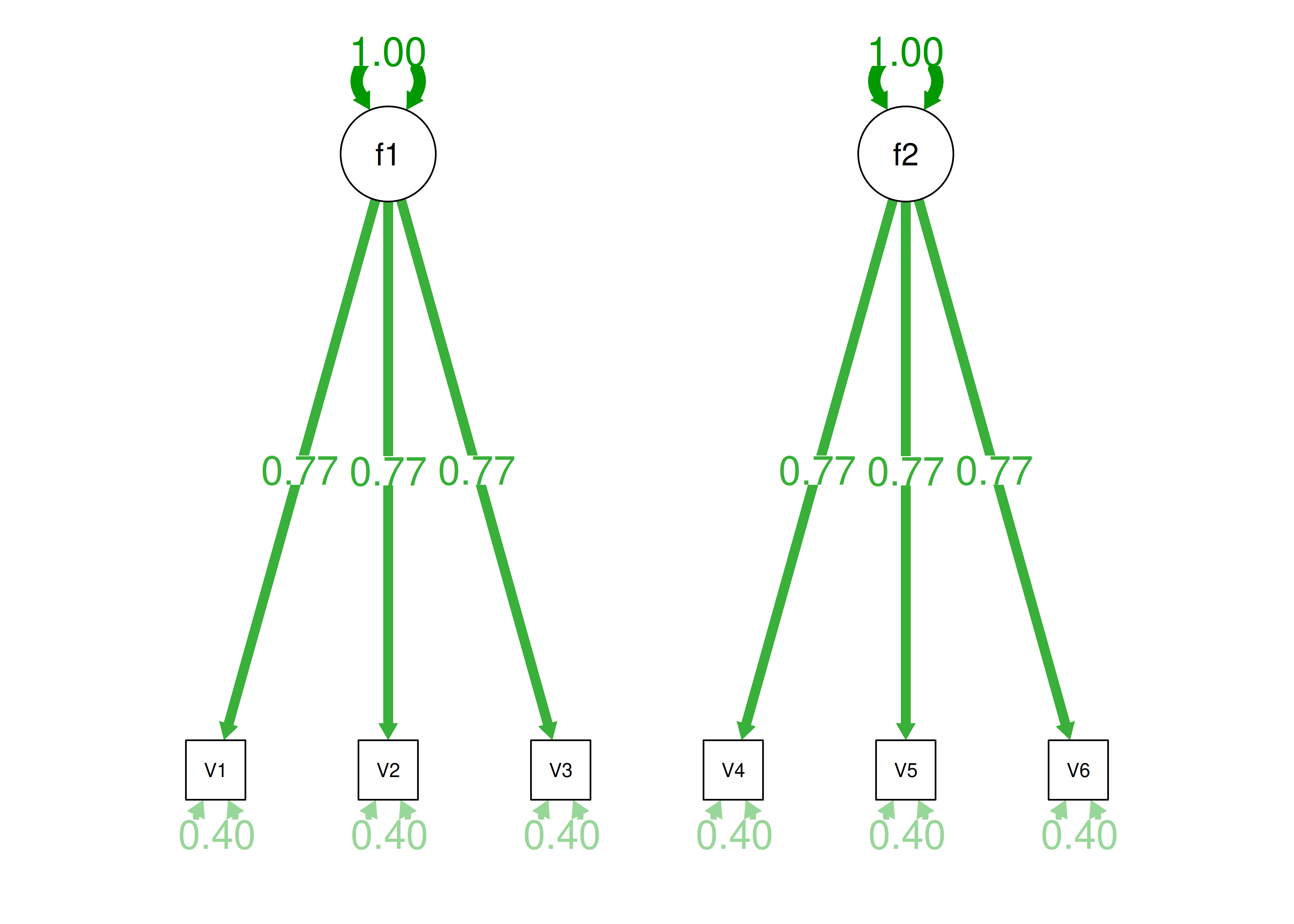
Figure 14.52: Confirmatory Factor Analysis Model 3b Diagram.
14.4.2.10.5 Create the covariance matrix
Code
correlationMatrixModel4 <- matrix(c(
1,.6,.6,.3,.3,.3,
.6,1,.6,.3,.3,.3,
.3,.3,1,.3,.3,.3,
.3,.3,.3,1,.6,.6,
.3,.3,.3,.6,1,.6,
.3,.3,.3,.6,.6,1),
nrow = 6,
ncol = 6)
rownames(correlationMatrixModel4) <- colnames(correlationMatrixModel4) <-
paste("V", 1:6, sep = "")
covarianceMatrixModel4 <- psych::cor2cov(
correlationMatrixModel4,
sigma = standardDeviations)
covarianceMatrixModel4 V1 V2 V3 V4 V5 V6
V1 1.0 0.6 0.3 0.3 0.3 0.3
V2 0.6 1.0 0.3 0.3 0.3 0.3
V3 0.6 0.6 1.0 0.3 0.3 0.3
V4 0.3 0.3 0.3 1.0 0.6 0.6
V5 0.3 0.3 0.3 0.6 1.0 0.6
V6 0.3 0.3 0.3 0.6 0.6 1.014.4.2.10.5.1 Specify the model
Code
cfaModel4A <- '
#Factor loadings
f1 =~ V1 + V2 + V3
f2 =~ V4 + V5 + V6
'
cfaModel4B <- '
#Factor loadings
f1 =~ V1 + V2 + V3
f2 =~ V4 + V5 + V6
#Regression path
f2 ~ f1
'
cfaModel4C <- '
#Factor loadings
f1 =~ V1 + V2 + V3
f2 =~ V4 + V5 + V6
#Higher-order factor
A1 = ~ fixloading*f1 + fixloading*f2
'
cfaModel4D <- '
#Factor loadings
f1 =~ V1 + V2 + V3 + V4 + V5 + V6
#Correlated residuals/errors
V1 ~~ fixcor*V2
V2 ~~ fixcor*V3
V1 ~~ fixcor*V3
V4 ~~ fixcor*V5
V5 ~~ fixcor*V6
V4 ~~ fixcor*V6
'
cfaModel4E <- '
#Factor loadings
f1 =~ V1 + V2 + V3 + V4 + V5 + V6 #construct latent factor
f2 =~ fixloading*V4 + fixloading*V5 + fixloading*V6 #method latent factor
#Make construct and method latent factors orthogonal (uncorrelated)
f1 ~~ 0*f2
'14.4.2.10.5.3 Fit the model
Code
cfaModel4AFit <- cfa(
cfaModel4A,
sample.cov = covarianceMatrixModel4,
sample.nobs = sampleSize,
estimator = "ML",
std.lv = TRUE)
cfaModel4BFit <- cfa(
cfaModel4B,
sample.cov = covarianceMatrixModel4,
sample.nobs = sampleSize,
estimator = "ML",
std.lv = TRUE)
cfaModel4CFit <- cfa(
cfaModel4C,
sample.cov = covarianceMatrixModel4,
sample.nobs = sampleSize,
estimator = "ML",
std.lv = TRUE)
cfaModel4DFit <- cfa(
cfaModel4D,
sample.cov = covarianceMatrixModel4,
sample.nobs = sampleSize,
estimator = "ML",
std.lv = TRUE)
cfaModel4EFit <- cfa(
cfaModel4E,
sample.cov = covarianceMatrixModel4,
sample.nobs = sampleSize,
estimator = "ML",
std.lv = TRUE)14.4.2.10.5.4 Display summary output
lavaan 0.6-20 ended normally after 9 iterations
Estimator ML
Optimization method NLMINB
Number of model parameters 13
Number of observations 300
Model Test User Model:
Test statistic 0.000
Degrees of freedom 8
P-value (Chi-square) 1.000
Model Test Baseline Model:
Test statistic 681.419
Degrees of freedom 15
P-value 0.000
User Model versus Baseline Model:
Comparative Fit Index (CFI) 1.000
Tucker-Lewis Index (TLI) 1.023
Loglikelihood and Information Criteria:
Loglikelihood user model (H0) -2210.375
Loglikelihood unrestricted model (H1) -2210.375
Akaike (AIC) 4446.750
Bayesian (BIC) 4494.899
Sample-size adjusted Bayesian (SABIC) 4453.671
Root Mean Square Error of Approximation:
RMSEA 0.000
90 Percent confidence interval - lower 0.000
90 Percent confidence interval - upper 0.000
P-value H_0: RMSEA <= 0.050 1.000
P-value H_0: RMSEA >= 0.080 0.000
Standardized Root Mean Square Residual:
SRMR 0.000
Parameter Estimates:
Standard errors Standard
Information Expected
Information saturated (h1) model Structured
Latent Variables:
Estimate Std.Err z-value P(>|z|) Std.lv Std.all
f1 =~
V1 0.773 0.054 14.351 0.000 0.773 0.775
V2 0.773 0.054 14.351 0.000 0.773 0.775
V3 0.773 0.054 14.351 0.000 0.773 0.775
f2 =~
V4 0.773 0.054 14.351 0.000 0.773 0.775
V5 0.773 0.054 14.351 0.000 0.773 0.775
V6 0.773 0.054 14.351 0.000 0.773 0.775
Covariances:
Estimate Std.Err z-value P(>|z|) Std.lv Std.all
f1 ~~
f2 0.500 0.057 8.822 0.000 0.500 0.500
Variances:
Estimate Std.Err z-value P(>|z|) Std.lv Std.all
.V1 0.399 0.049 8.067 0.000 0.399 0.400
.V2 0.399 0.049 8.067 0.000 0.399 0.400
.V3 0.399 0.049 8.067 0.000 0.399 0.400
.V4 0.399 0.049 8.067 0.000 0.399 0.400
.V5 0.399 0.049 8.067 0.000 0.399 0.400
.V6 0.399 0.049 8.067 0.000 0.399 0.400
f1 1.000 1.000 1.000
f2 1.000 1.000 1.000
R-Square:
Estimate
V1 0.600
V2 0.600
V3 0.600
V4 0.600
V5 0.600
V6 0.600lavaan 0.6-20 ended normally after 12 iterations
Estimator ML
Optimization method NLMINB
Number of model parameters 13
Number of observations 300
Model Test User Model:
Test statistic 0.000
Degrees of freedom 8
P-value (Chi-square) 1.000
Model Test Baseline Model:
Test statistic 681.419
Degrees of freedom 15
P-value 0.000
User Model versus Baseline Model:
Comparative Fit Index (CFI) 1.000
Tucker-Lewis Index (TLI) 1.023
Loglikelihood and Information Criteria:
Loglikelihood user model (H0) -2210.375
Loglikelihood unrestricted model (H1) -2210.375
Akaike (AIC) 4446.750
Bayesian (BIC) 4494.899
Sample-size adjusted Bayesian (SABIC) 4453.671
Root Mean Square Error of Approximation:
RMSEA 0.000
90 Percent confidence interval - lower 0.000
90 Percent confidence interval - upper 0.000
P-value H_0: RMSEA <= 0.050 1.000
P-value H_0: RMSEA >= 0.080 0.000
Standardized Root Mean Square Residual:
SRMR 0.000
Parameter Estimates:
Standard errors Standard
Information Expected
Information saturated (h1) model Structured
Latent Variables:
Estimate Std.Err z-value P(>|z|) Std.lv Std.all
f1 =~
V1 0.773 0.054 14.351 0.000 0.773 0.775
V2 0.773 0.054 14.351 0.000 0.773 0.775
V3 0.773 0.054 14.351 0.000 0.773 0.775
f2 =~
V4 0.670 0.050 13.445 0.000 0.773 0.775
V5 0.670 0.050 13.445 0.000 0.773 0.775
V6 0.670 0.050 13.445 0.000 0.773 0.775
Regressions:
Estimate Std.Err z-value P(>|z|) Std.lv Std.all
f2 ~
f1 0.577 0.087 6.616 0.000 0.500 0.500
Variances:
Estimate Std.Err z-value P(>|z|) Std.lv Std.all
.V1 0.399 0.049 8.067 0.000 0.399 0.400
.V2 0.399 0.049 8.067 0.000 0.399 0.400
.V3 0.399 0.049 8.067 0.000 0.399 0.400
.V4 0.399 0.049 8.067 0.000 0.399 0.400
.V5 0.399 0.049 8.067 0.000 0.399 0.400
.V6 0.399 0.049 8.067 0.000 0.399 0.400
f1 1.000 1.000 1.000
.f2 1.000 0.750 0.750
R-Square:
Estimate
V1 0.600
V2 0.600
V3 0.600
V4 0.600
V5 0.600
V6 0.600
f2 0.250lavaan 0.6-20 ended normally after 15 iterations
Estimator ML
Optimization method NLMINB
Number of model parameters 14
Number of equality constraints 1
Number of observations 300
Model Test User Model:
Test statistic 0.000
Degrees of freedom 8
P-value (Chi-square) 1.000
Model Test Baseline Model:
Test statistic 681.419
Degrees of freedom 15
P-value 0.000
User Model versus Baseline Model:
Comparative Fit Index (CFI) 1.000
Tucker-Lewis Index (TLI) 1.023
Loglikelihood and Information Criteria:
Loglikelihood user model (H0) -2210.375
Loglikelihood unrestricted model (H1) -2210.375
Akaike (AIC) 4446.750
Bayesian (BIC) 4494.899
Sample-size adjusted Bayesian (SABIC) 4453.671
Root Mean Square Error of Approximation:
RMSEA 0.000
90 Percent confidence interval - lower 0.000
90 Percent confidence interval - upper 0.000
P-value H_0: RMSEA <= 0.050 1.000
P-value H_0: RMSEA >= 0.080 0.000
Standardized Root Mean Square Residual:
SRMR 0.000
Parameter Estimates:
Standard errors Standard
Information Expected
Information saturated (h1) model Structured
Latent Variables:
Estimate Std.Err z-value P(>|z|) Std.lv Std.all
f1 =~
V1 0.547 0.046 12.003 0.000 0.773 0.775
V2 0.547 0.046 12.003 0.000 0.773 0.775
V3 0.547 0.046 12.003 0.000 0.773 0.775
f2 =~
V4 0.547 0.046 12.003 0.000 0.773 0.775
V5 0.547 0.046 12.003 0.000 0.773 0.775
V6 0.547 0.046 12.003 0.000 0.773 0.775
A1 =~
f1 (fxld) 1.000 0.113 8.822 0.000 0.707 0.707
f2 (fxld) 1.000 0.113 8.822 0.000 0.707 0.707
Variances:
Estimate Std.Err z-value P(>|z|) Std.lv Std.all
.V1 0.399 0.049 8.067 0.000 0.399 0.400
.V2 0.399 0.049 8.067 0.000 0.399 0.400
.V3 0.399 0.049 8.067 0.000 0.399 0.400
.V4 0.399 0.049 8.067 0.000 0.399 0.400
.V5 0.399 0.049 8.067 0.000 0.399 0.400
.V6 0.399 0.049 8.067 0.000 0.399 0.400
.f1 1.000 0.500 0.500
.f2 1.000 0.500 0.500
A1 1.000 1.000 1.000
R-Square:
Estimate
V1 0.600
V2 0.600
V3 0.600
V4 0.600
V5 0.600
V6 0.600
f1 0.500
f2 0.500lavaan 0.6-20 ended normally after 17 iterations
Estimator ML
Optimization method NLMINB
Number of model parameters 18
Number of equality constraints 5
Number of observations 300
Model Test User Model:
Test statistic 0.000
Degrees of freedom 8
P-value (Chi-square) 1.000
Model Test Baseline Model:
Test statistic 681.419
Degrees of freedom 15
P-value 0.000
User Model versus Baseline Model:
Comparative Fit Index (CFI) 1.000
Tucker-Lewis Index (TLI) 1.023
Loglikelihood and Information Criteria:
Loglikelihood user model (H0) -2210.375
Loglikelihood unrestricted model (H1) -2210.375
Akaike (AIC) 4446.750
Bayesian (BIC) 4494.899
Sample-size adjusted Bayesian (SABIC) 4453.671
Root Mean Square Error of Approximation:
RMSEA 0.000
90 Percent confidence interval - lower 0.000
90 Percent confidence interval - upper 0.000
P-value H_0: RMSEA <= 0.050 1.000
P-value H_0: RMSEA >= 0.080 0.000
Standardized Root Mean Square Residual:
SRMR 0.000
Parameter Estimates:
Standard errors Standard
Information Expected
Information saturated (h1) model Structured
Latent Variables:
Estimate Std.Err z-value P(>|z|) Std.lv Std.all
f1 =~
V1 0.547 0.068 7.994 0.000 0.547 0.548
V2 0.547 0.068 7.994 0.000 0.547 0.548
V3 0.547 0.068 7.994 0.000 0.547 0.548
V4 0.547 0.068 7.994 0.000 0.547 0.548
V5 0.547 0.068 7.994 0.000 0.547 0.548
V6 0.547 0.068 7.994 0.000 0.547 0.548
Covariances:
Estimate Std.Err z-value P(>|z|) Std.lv Std.all
.V1 ~~
.V2 (fxcr) 0.299 0.036 8.380 0.000 0.299 0.429
.V2 ~~
.V3 (fxcr) 0.299 0.036 8.380 0.000 0.299 0.429
.V1 ~~
.V3 (fxcr) 0.299 0.036 8.380 0.000 0.299 0.429
.V4 ~~
.V5 (fxcr) 0.299 0.036 8.380 0.000 0.299 0.429
.V5 ~~
.V6 (fxcr) 0.299 0.036 8.380 0.000 0.299 0.429
.V4 ~~
.V6 (fxcr) 0.299 0.036 8.380 0.000 0.299 0.429
Variances:
Estimate Std.Err z-value P(>|z|) Std.lv Std.all
.V1 0.698 0.057 12.244 0.000 0.698 0.700
.V2 0.698 0.057 12.244 0.000 0.698 0.700
.V3 0.698 0.057 12.244 0.000 0.698 0.700
.V4 0.698 0.057 12.244 0.000 0.698 0.700
.V5 0.698 0.057 12.244 0.000 0.698 0.700
.V6 0.698 0.057 12.244 0.000 0.698 0.700
f1 1.000 1.000 1.000
R-Square:
Estimate
V1 0.300
V2 0.300
V3 0.300
V4 0.300
V5 0.300
V6 0.300lavaan 0.6-20 ended normally after 13 iterations
Estimator ML
Optimization method NLMINB
Number of model parameters 15
Number of equality constraints 2
Number of observations 300
Model Test User Model:
Test statistic 0.000
Degrees of freedom 8
P-value (Chi-square) 1.000
Model Test Baseline Model:
Test statistic 681.419
Degrees of freedom 15
P-value 0.000
User Model versus Baseline Model:
Comparative Fit Index (CFI) 1.000
Tucker-Lewis Index (TLI) 1.023
Loglikelihood and Information Criteria:
Loglikelihood user model (H0) -2210.375
Loglikelihood unrestricted model (H1) -2210.375
Akaike (AIC) 4446.750
Bayesian (BIC) 4494.899
Sample-size adjusted Bayesian (SABIC) 4453.671
Root Mean Square Error of Approximation:
RMSEA 0.000
90 Percent confidence interval - lower 0.000
90 Percent confidence interval - upper 0.000
P-value H_0: RMSEA <= 0.050 1.000
P-value H_0: RMSEA >= 0.080 0.000
Standardized Root Mean Square Residual:
SRMR 0.000
Parameter Estimates:
Standard errors Standard
Information Expected
Information saturated (h1) model Structured
Latent Variables:
Estimate Std.Err z-value P(>|z|) Std.lv Std.all
f1 =~
V1 0.773 0.054 14.351 0.000 0.773 0.775
V2 0.773 0.054 14.351 0.000 0.773 0.775
V3 0.773 0.054 14.351 0.000 0.773 0.775
V4 0.387 0.061 6.347 0.000 0.387 0.387
V5 0.387 0.061 6.347 0.000 0.387 0.387
V6 0.387 0.061 6.347 0.000 0.387 0.387
f2 =~
V4 (fxld) 0.670 0.038 17.657 0.000 0.670 0.671
V5 (fxld) 0.670 0.038 17.657 0.000 0.670 0.671
V6 (fxld) 0.670 0.038 17.657 0.000 0.670 0.671
Covariances:
Estimate Std.Err z-value P(>|z|) Std.lv Std.all
f1 ~~
f2 0.000 0.000 0.000
Variances:
Estimate Std.Err z-value P(>|z|) Std.lv Std.all
.V1 0.399 0.049 8.067 0.000 0.399 0.400
.V2 0.399 0.049 8.067 0.000 0.399 0.400
.V3 0.399 0.049 8.067 0.000 0.399 0.400
.V4 0.399 0.045 8.894 0.000 0.399 0.400
.V5 0.399 0.045 8.894 0.000 0.399 0.400
.V6 0.399 0.045 8.894 0.000 0.399 0.400
f1 1.000 1.000 1.000
f2 1.000 1.000 1.000
R-Square:
Estimate
V1 0.600
V2 0.600
V3 0.600
V4 0.600
V5 0.600
V6 0.60014.4.2.10.5.5 Estimates of model fit
Code
chisq df pvalue rmsea cfi tli srmr
0.000 8.000 1.000 0.000 1.000 1.023 0.000 Code
chisq df pvalue rmsea cfi tli srmr
0.000 8.000 1.000 0.000 1.000 1.023 0.000 Code
chisq df pvalue rmsea cfi tli srmr
0.000 8.000 1.000 0.000 1.000 1.023 0.000 Code
chisq df pvalue rmsea cfi tli srmr
0.000 8.000 1.000 0.000 1.000 1.023 0.000 Code
chisq df pvalue rmsea cfi tli srmr
0.000 8.000 1.000 0.000 1.000 1.023 0.000 14.4.2.10.5.6 Residuals
$type
[1] "cor.bollen"
$cov
V1 V2 V3 V4 V5 V6
V1 0
V2 0 0
V3 0 0 0
V4 0 0 0 0
V5 0 0 0 0 0
V6 0 0 0 0 0 0$type
[1] "cor.bollen"
$cov
V1 V2 V3 V4 V5 V6
V1 0
V2 0 0
V3 0 0 0
V4 0 0 0 0
V5 0 0 0 0 0
V6 0 0 0 0 0 0$type
[1] "cor.bollen"
$cov
V1 V2 V3 V4 V5 V6
V1 0
V2 0 0
V3 0 0 0
V4 0 0 0 0
V5 0 0 0 0 0
V6 0 0 0 0 0 0$type
[1] "cor.bollen"
$cov
V1 V2 V3 V4 V5 V6
V1 0
V2 0 0
V3 0 0 0
V4 0 0 0 0
V5 0 0 0 0 0
V6 0 0 0 0 0 0$type
[1] "cor.bollen"
$cov
V1 V2 V3 V4 V5 V6
V1 0
V2 0 0
V3 0 0 0
V4 0 0 0 0
V5 0 0 0 0 0
V6 0 0 0 0 0 014.4.2.10.5.8 Internal Consistency Reliability
Internal consistency reliability of items composing the latent factors, as quantified by omega (\(\omega\)) and average variance extracted (AVE), was estimated using the semTools package (Jorgensen et al., 2021).
f1 f2
0.818 0.818 f1 f2
0.818 0.818 f1 f2
0.818 0.818 f1 f2 A1
0.818 0.818 0.581 f1
0.581 f1 f2
0.653 0.614 f1 f2
0.6 0.6 f1 f2
0.6 0.6 f1 f2
0.6 0.6 f1
0.3 f1 f2
NA NA 14.4.2.10.5.9 Path diagram
Path diagrams of the models generated using the semPlot package (Epskamp, 2022) are in Figures 14.53, 14.54, 14.55, 14.56, and 14.57.
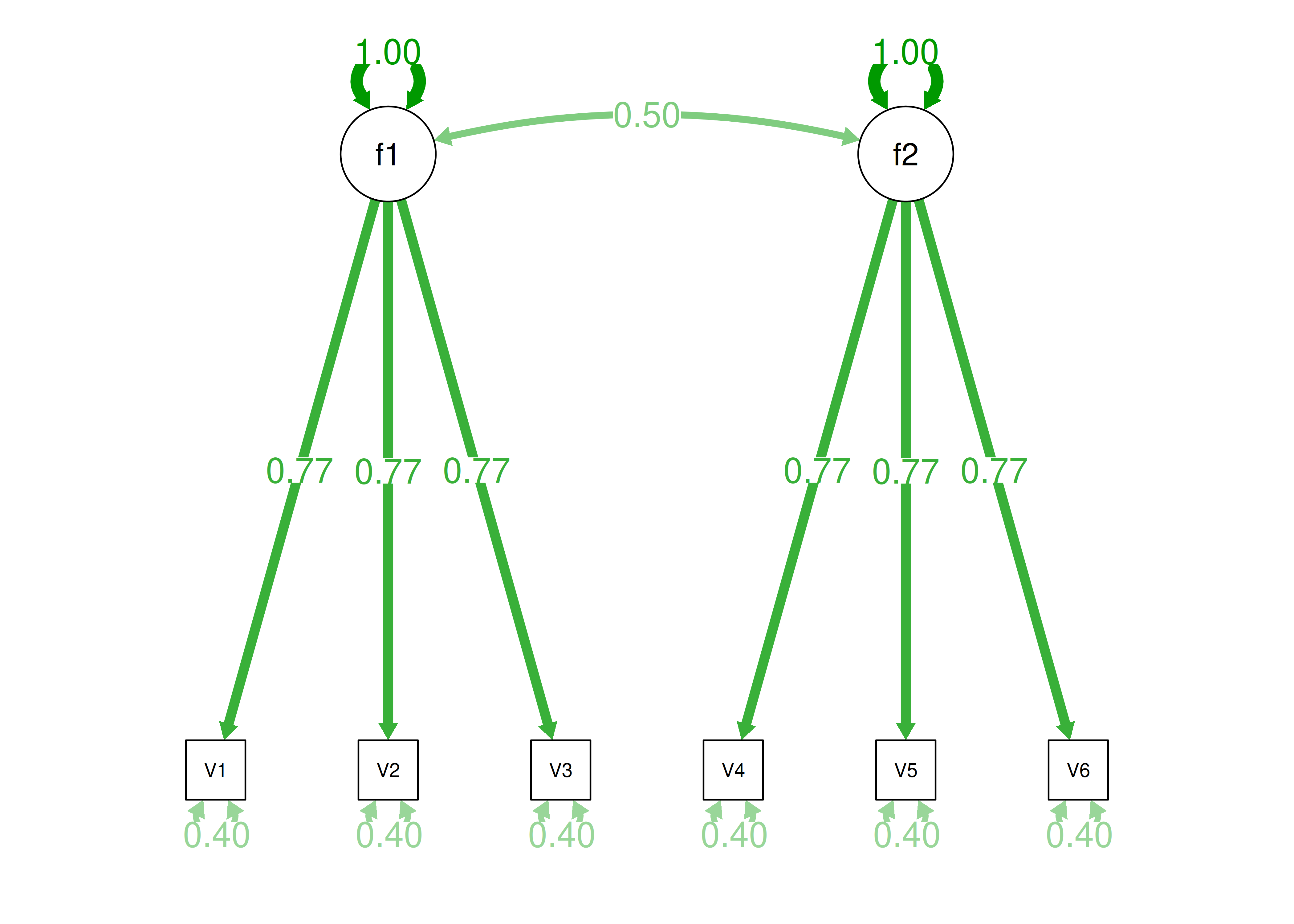
Figure 14.53: Confirmatory Factor Analysis Model 4a Diagram.
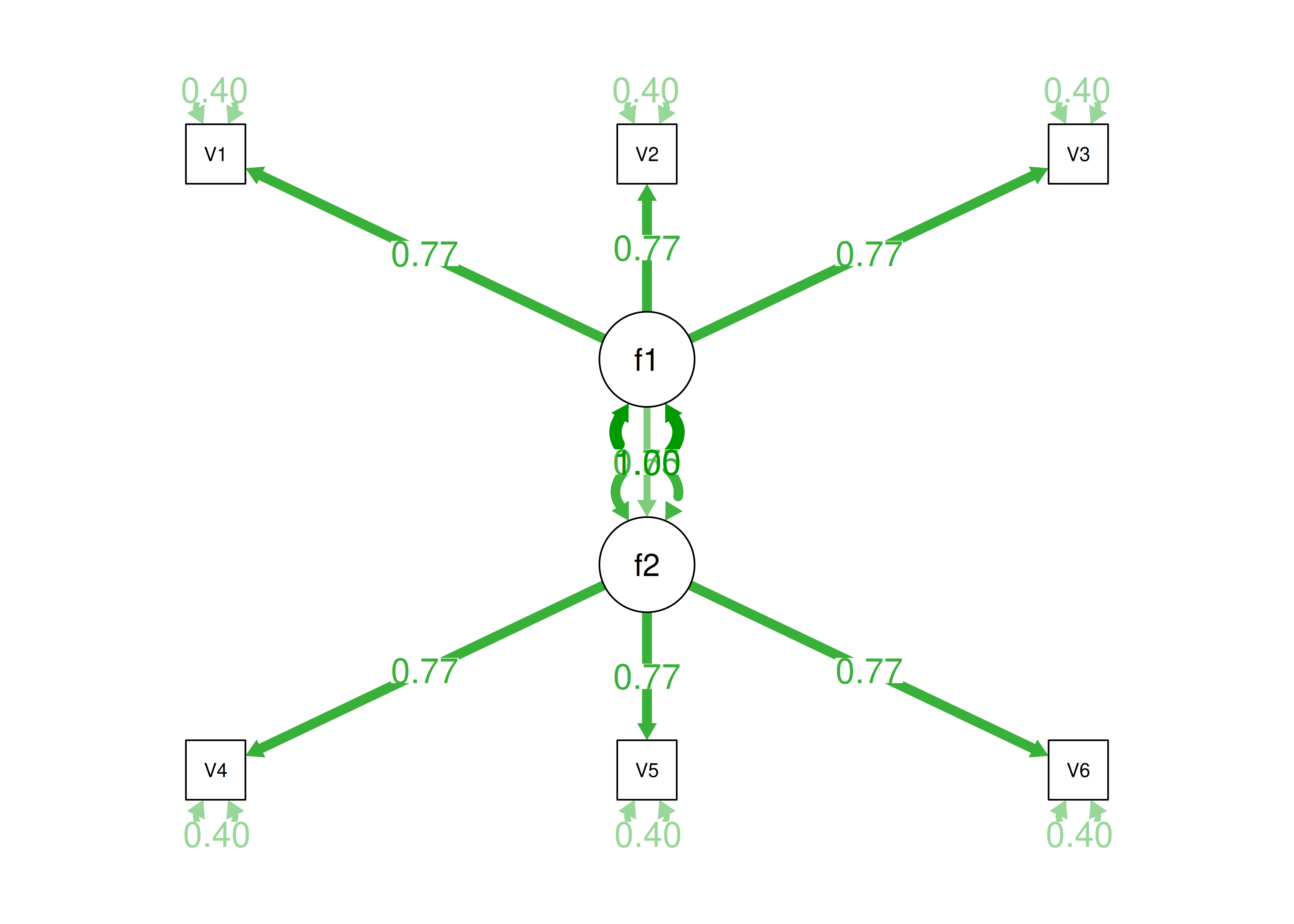
Figure 14.54: Confirmatory Factor Analysis Model 4b Diagram.
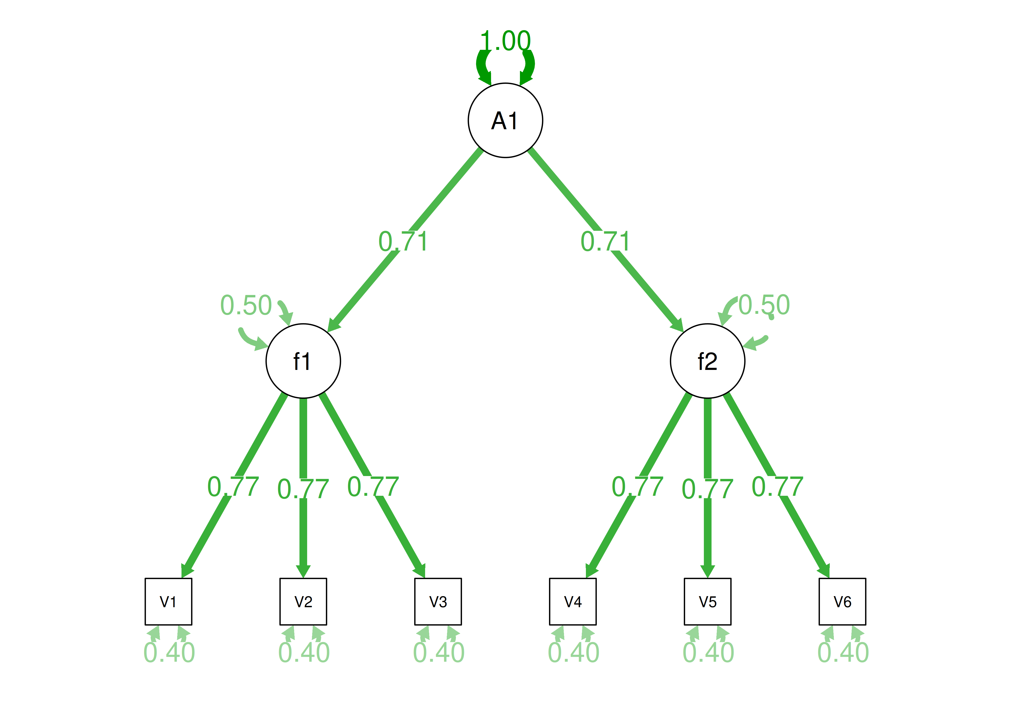
Figure 14.55: Confirmatory Factor Analysis Model 4c Diagram.
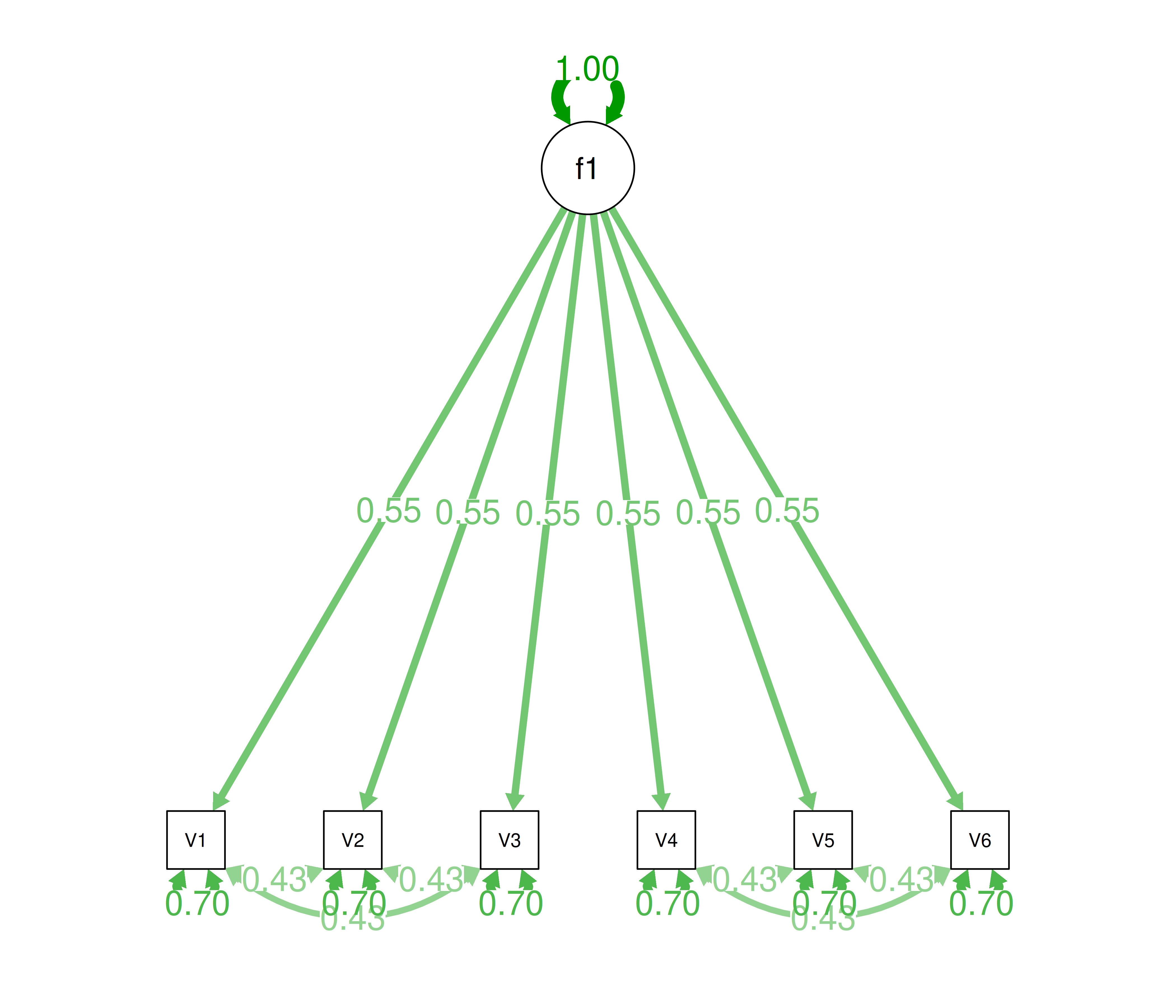
Figure 14.56: Confirmatory Factor Analysis Model 4d Diagram.
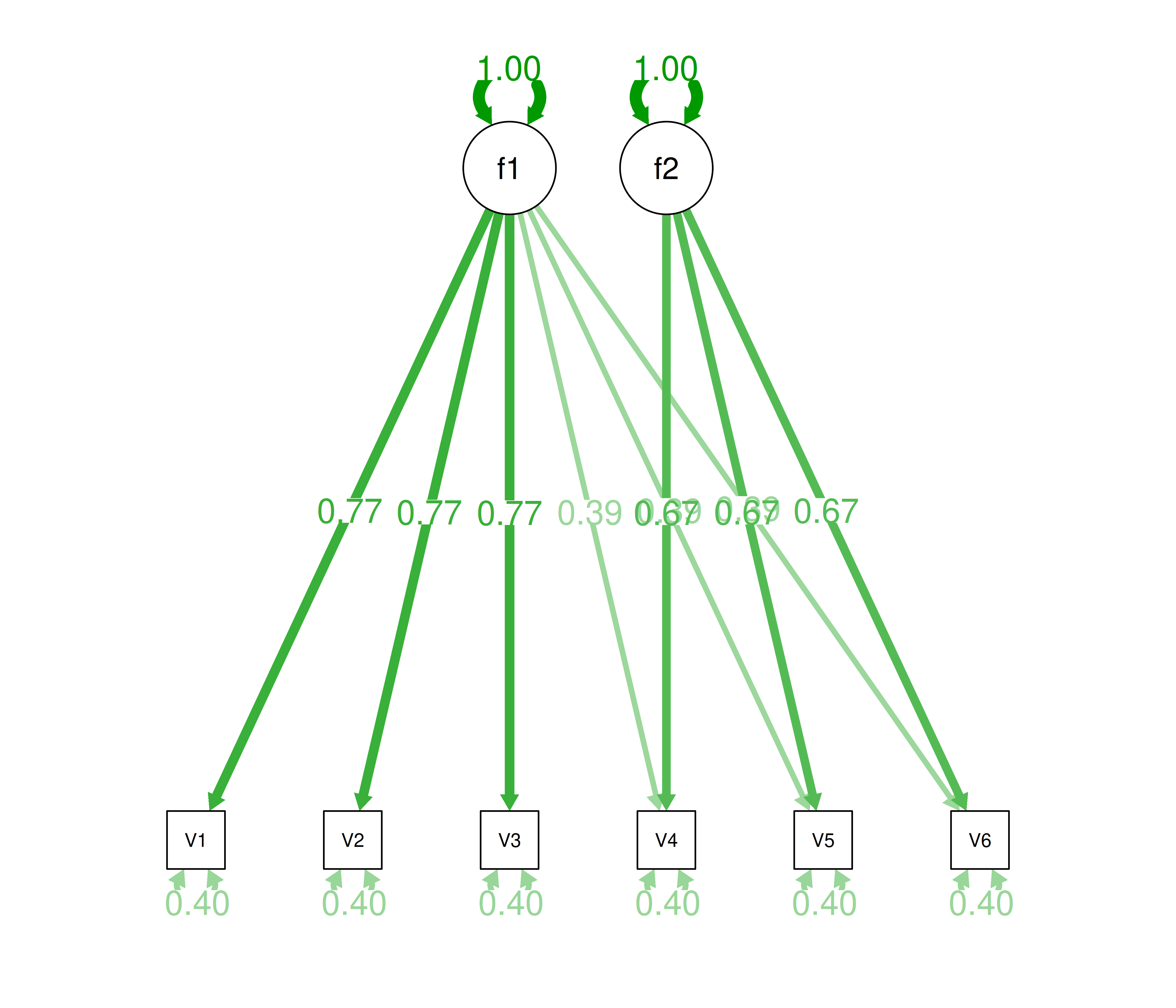
Figure 14.57: Confirmatory Factor Analysis Model 4e Diagram.
14.4.2.10.5.10 Equivalently fitting models
Markov equivalent directed acyclic graphs (DAGs) were depicted using the dagitty package (Textor et al., 2021).
Path diagrams of equivalent models are below.
Figure 14.58: Equivalently Fitting Models to Confirmatory Factor Analysis Model 4.

Figure 14.59: Equivalently Fitting Models to Confirmatory Factor Analysis Model 4.
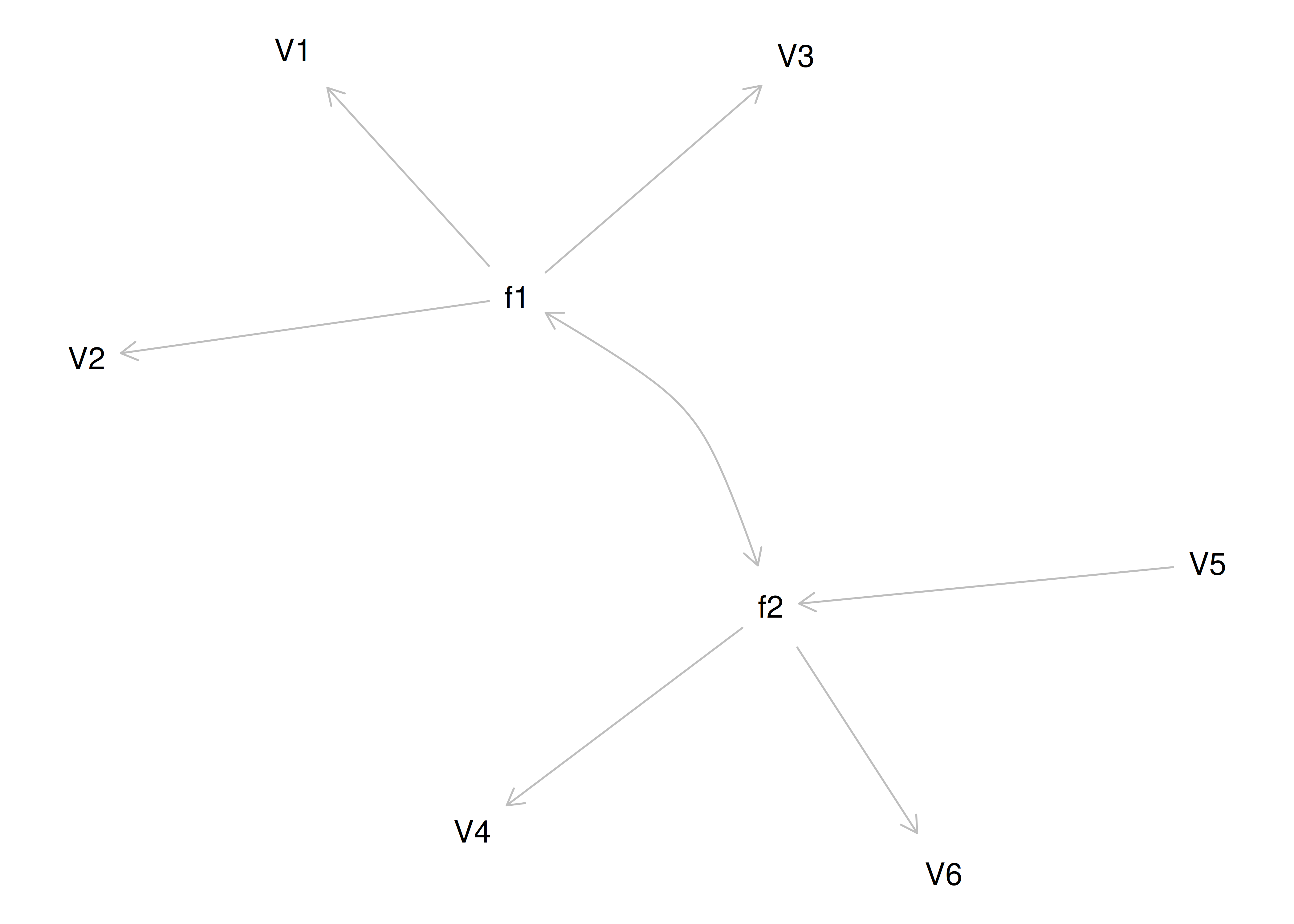
Figure 14.60: Equivalently Fitting Models to Confirmatory Factor Analysis Model 4.
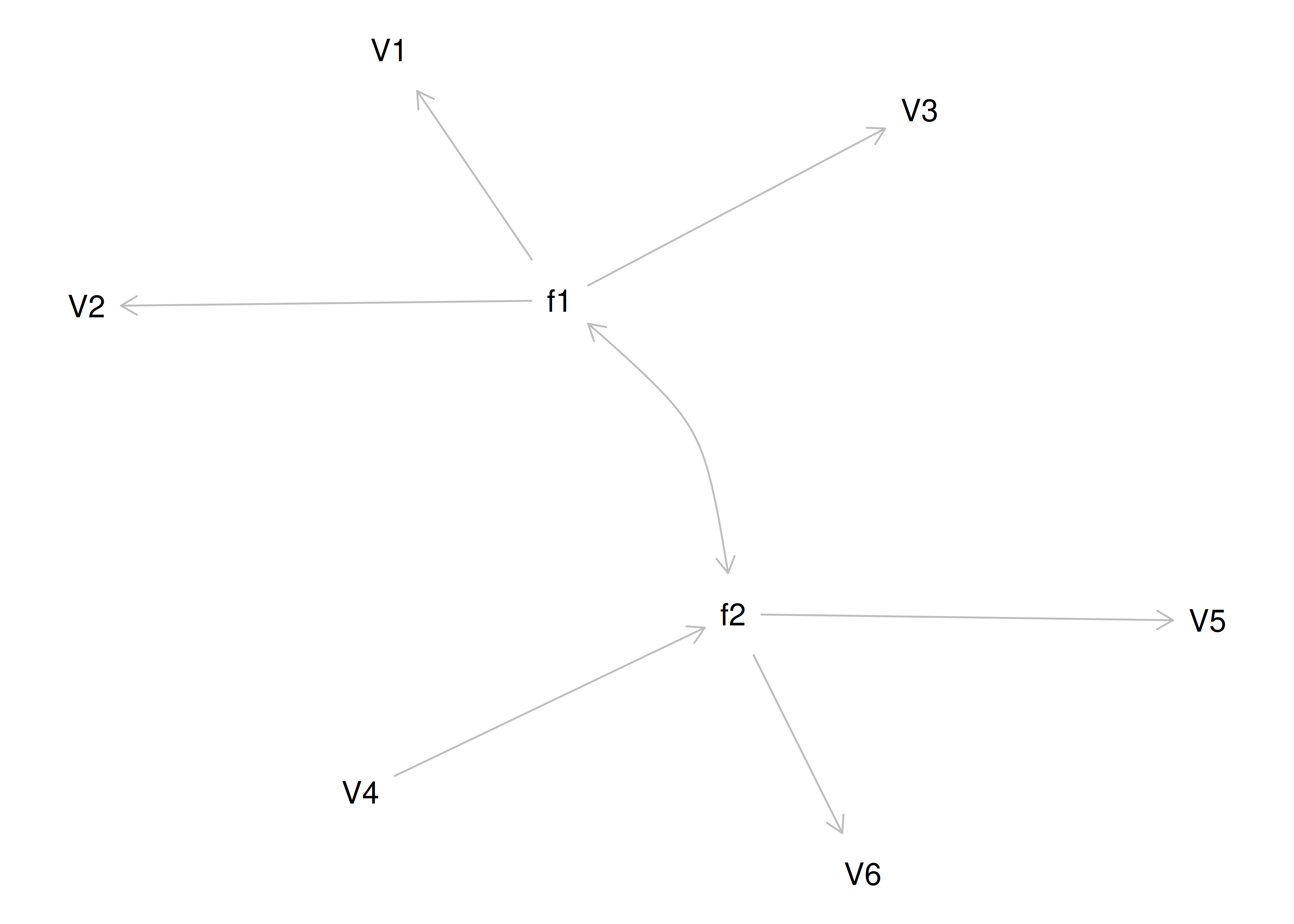
Figure 14.61: Equivalently Fitting Models to Confirmatory Factor Analysis Model 4.
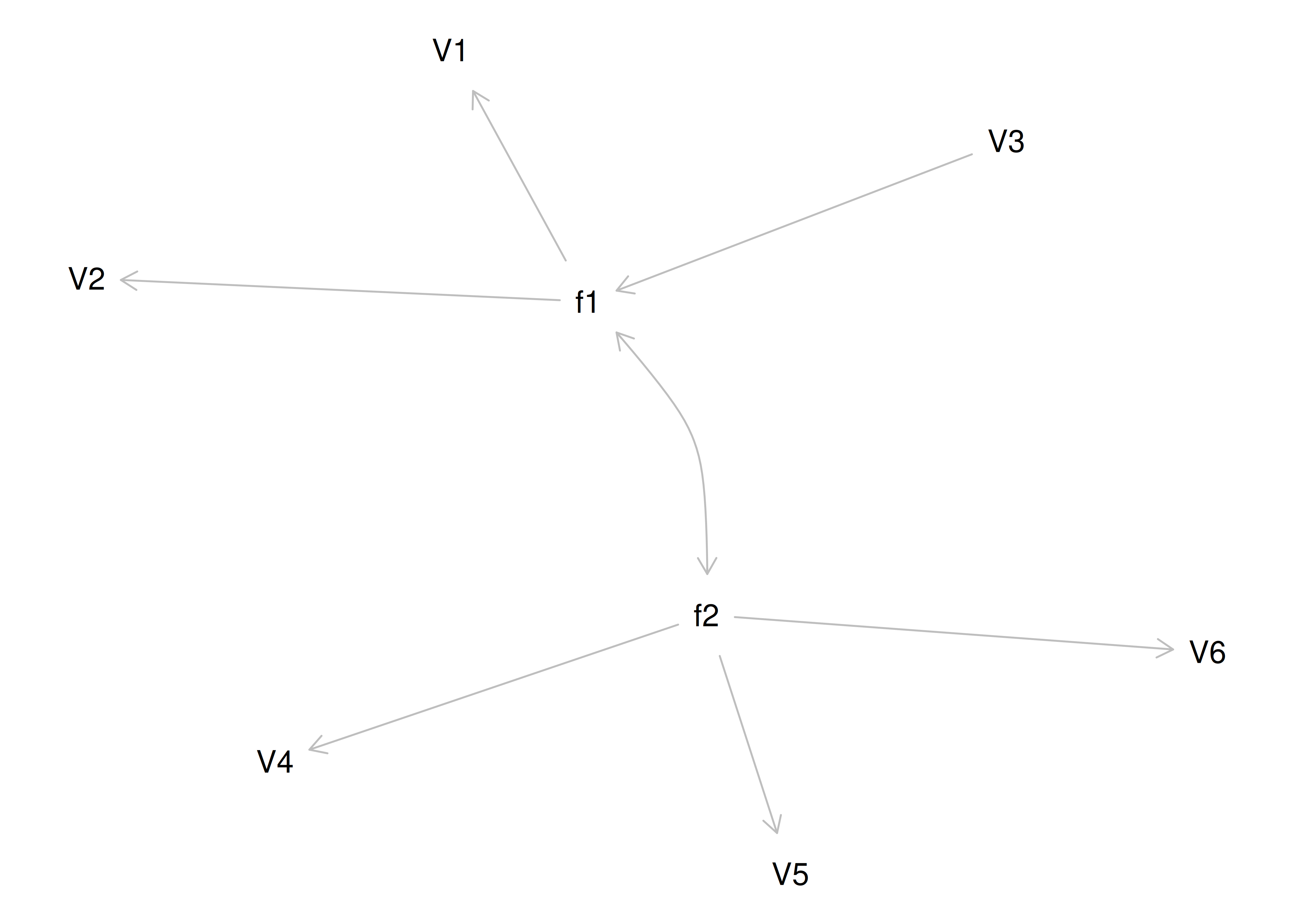
Figure 14.62: Equivalently Fitting Models to Confirmatory Factor Analysis Model 4.
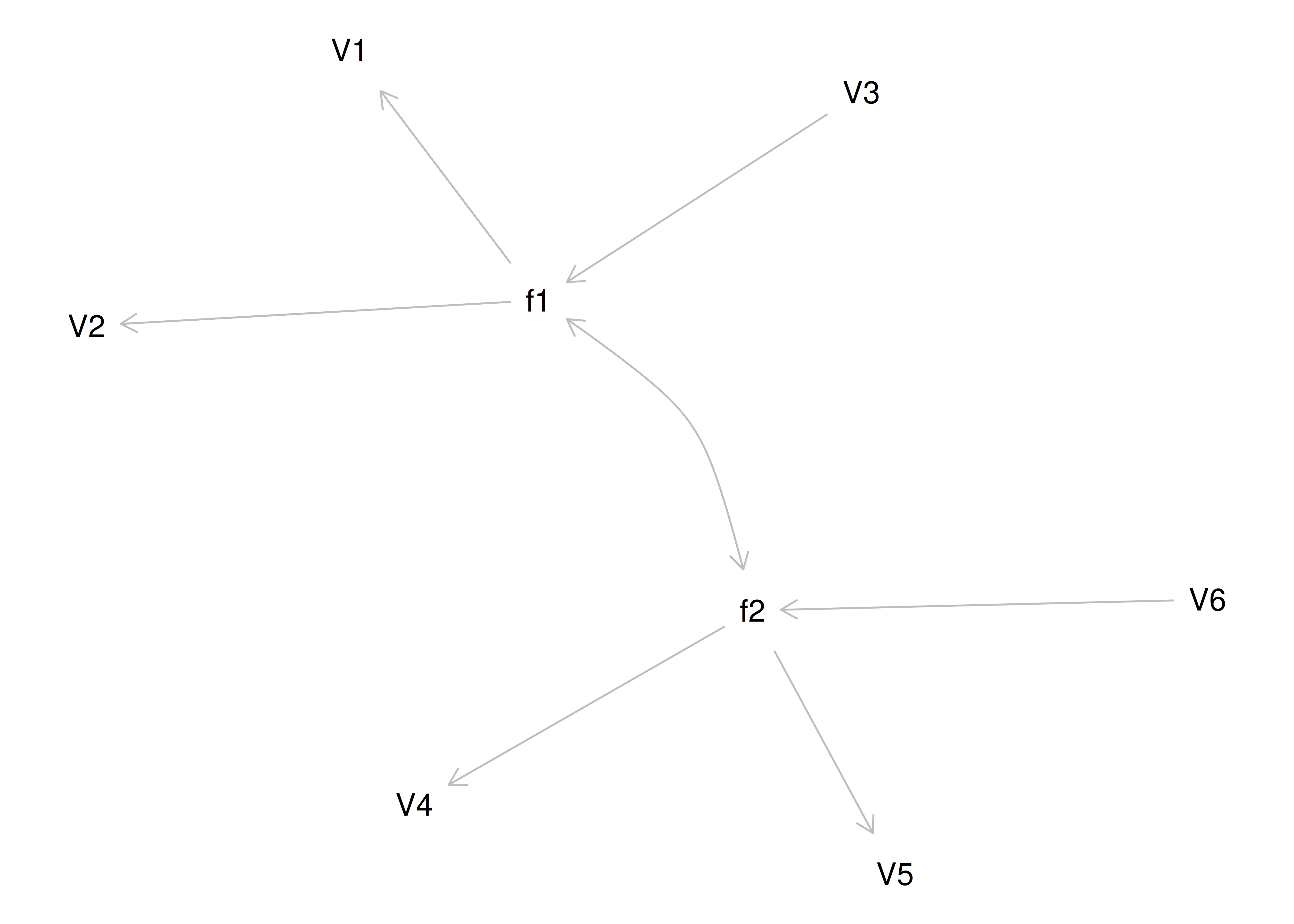
Figure 14.63: Equivalently Fitting Models to Confirmatory Factor Analysis Model 4.
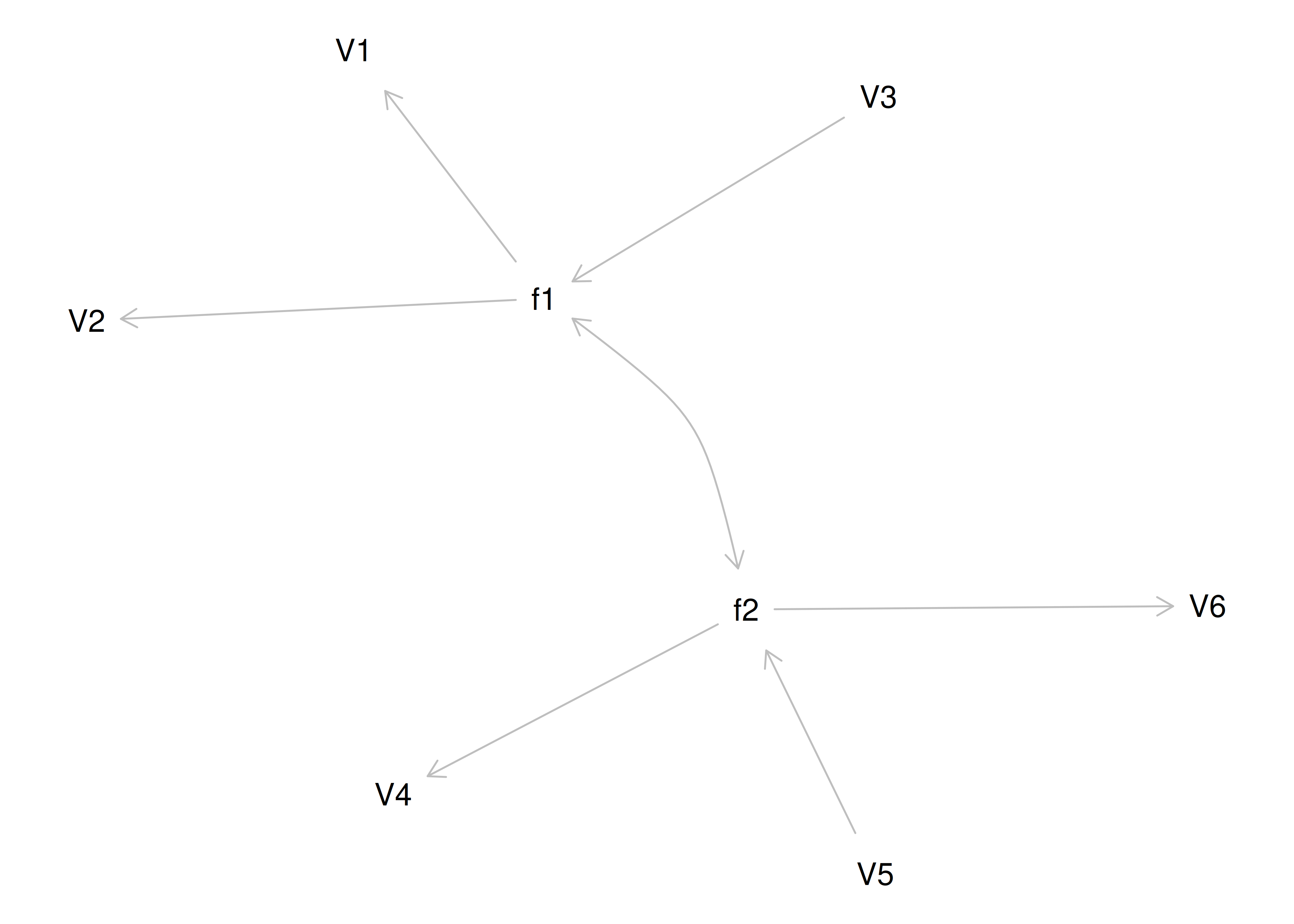
Figure 14.64: Equivalently Fitting Models to Confirmatory Factor Analysis Model 4.
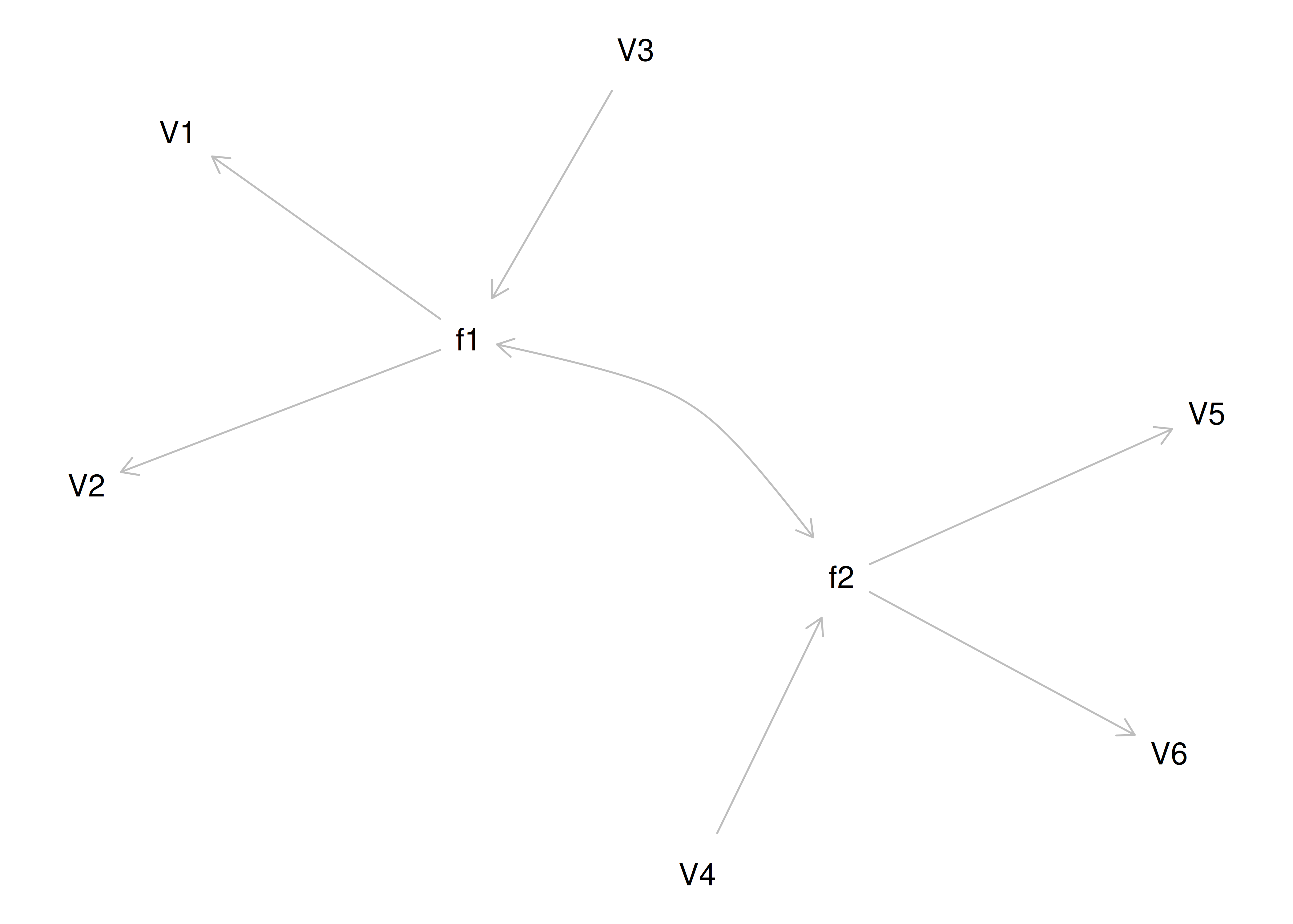
Figure 14.65: Equivalently Fitting Models to Confirmatory Factor Analysis Model 4.
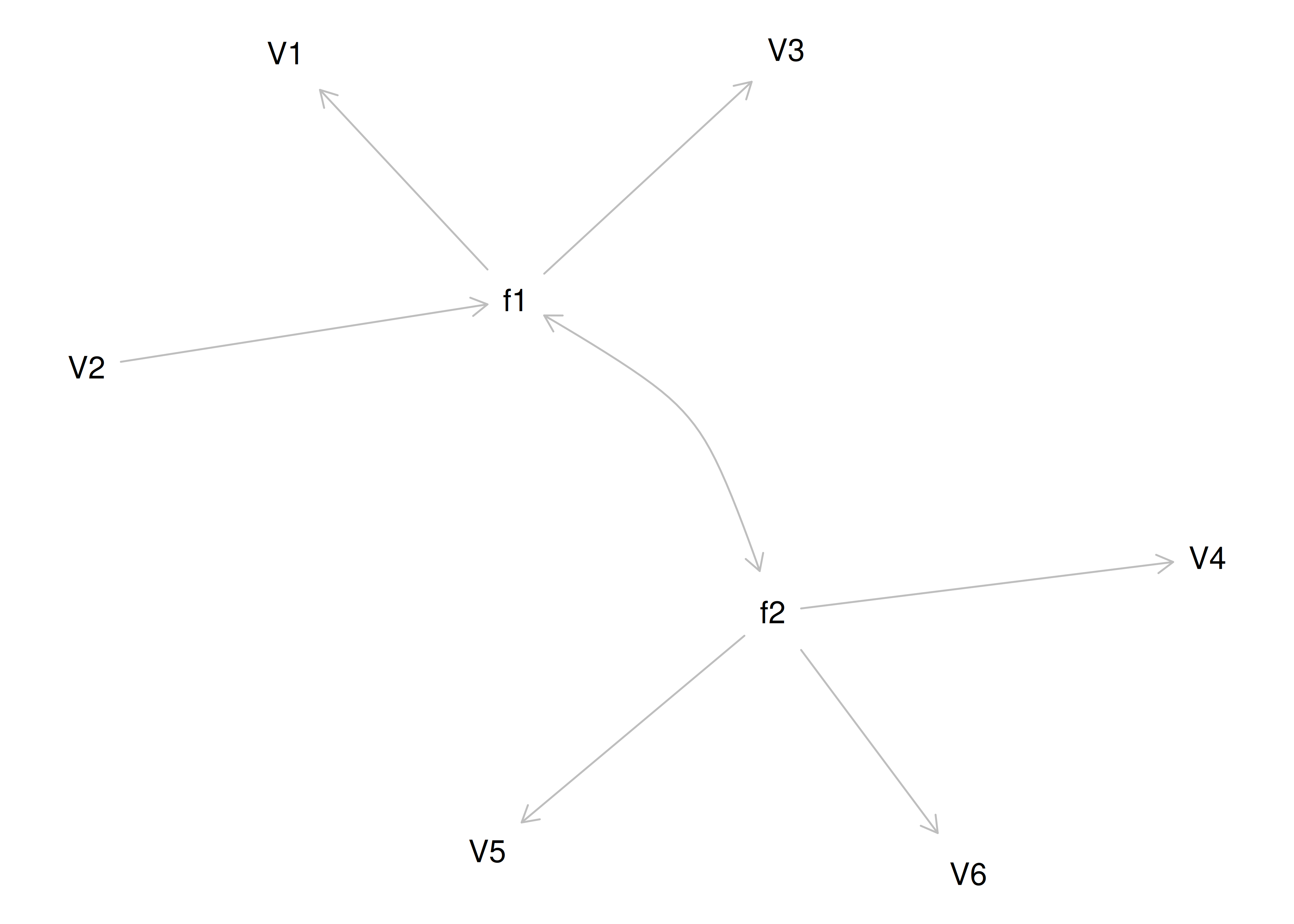
Figure 14.66: Equivalently Fitting Models to Confirmatory Factor Analysis Model 4.
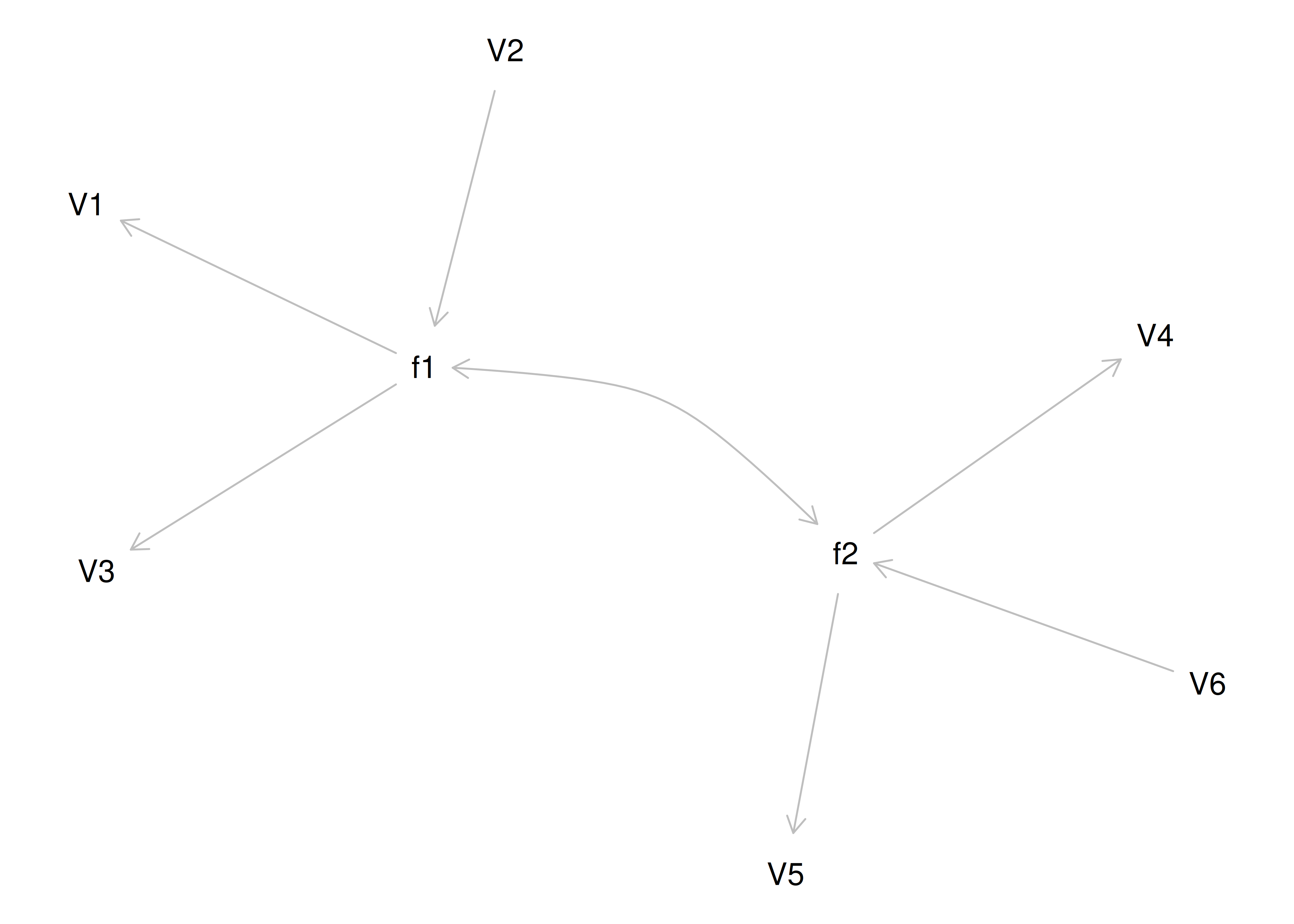
Figure 14.67: Equivalently Fitting Models to Confirmatory Factor Analysis Model 4.
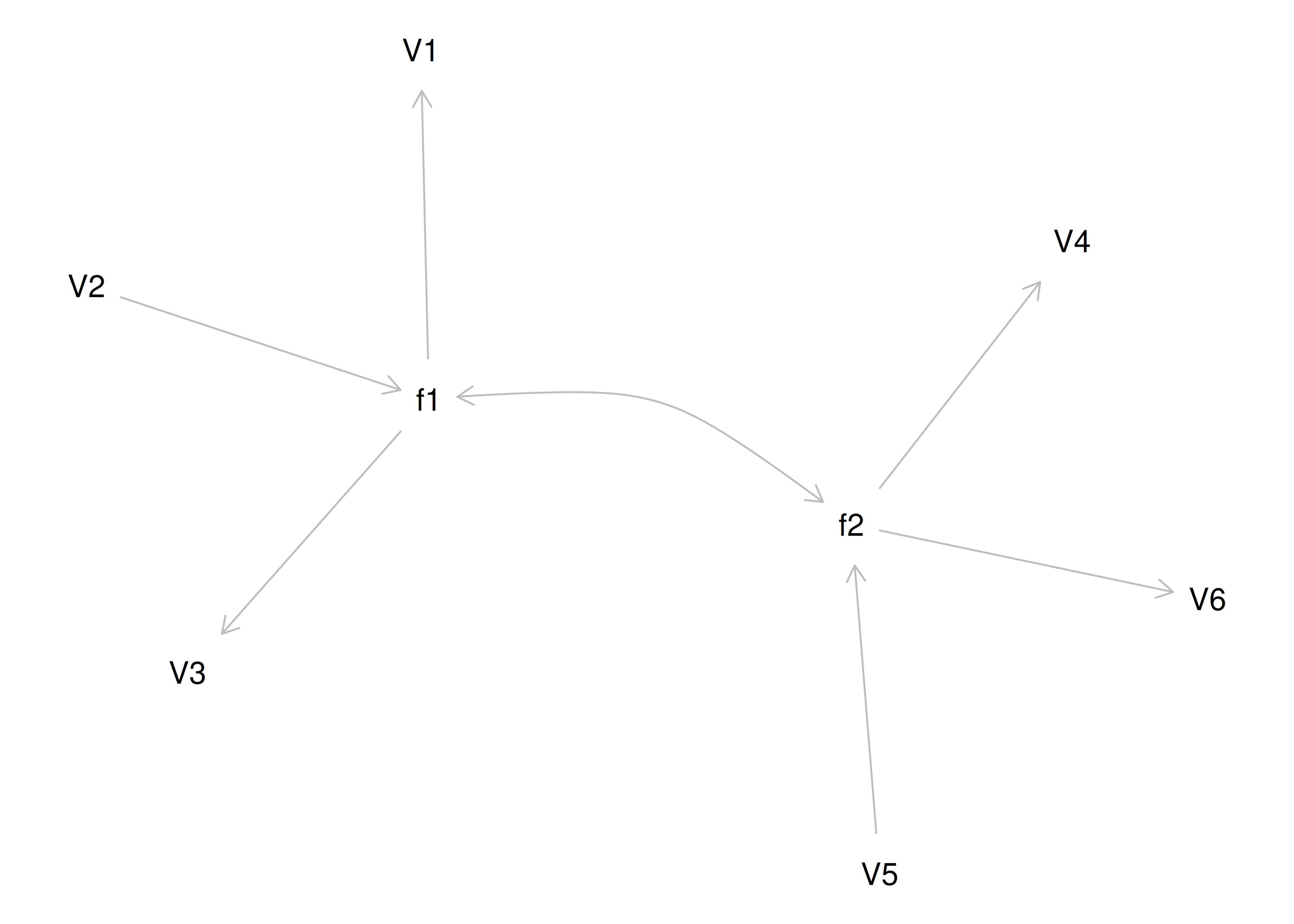
Figure 14.68: Equivalently Fitting Models to Confirmatory Factor Analysis Model 4.
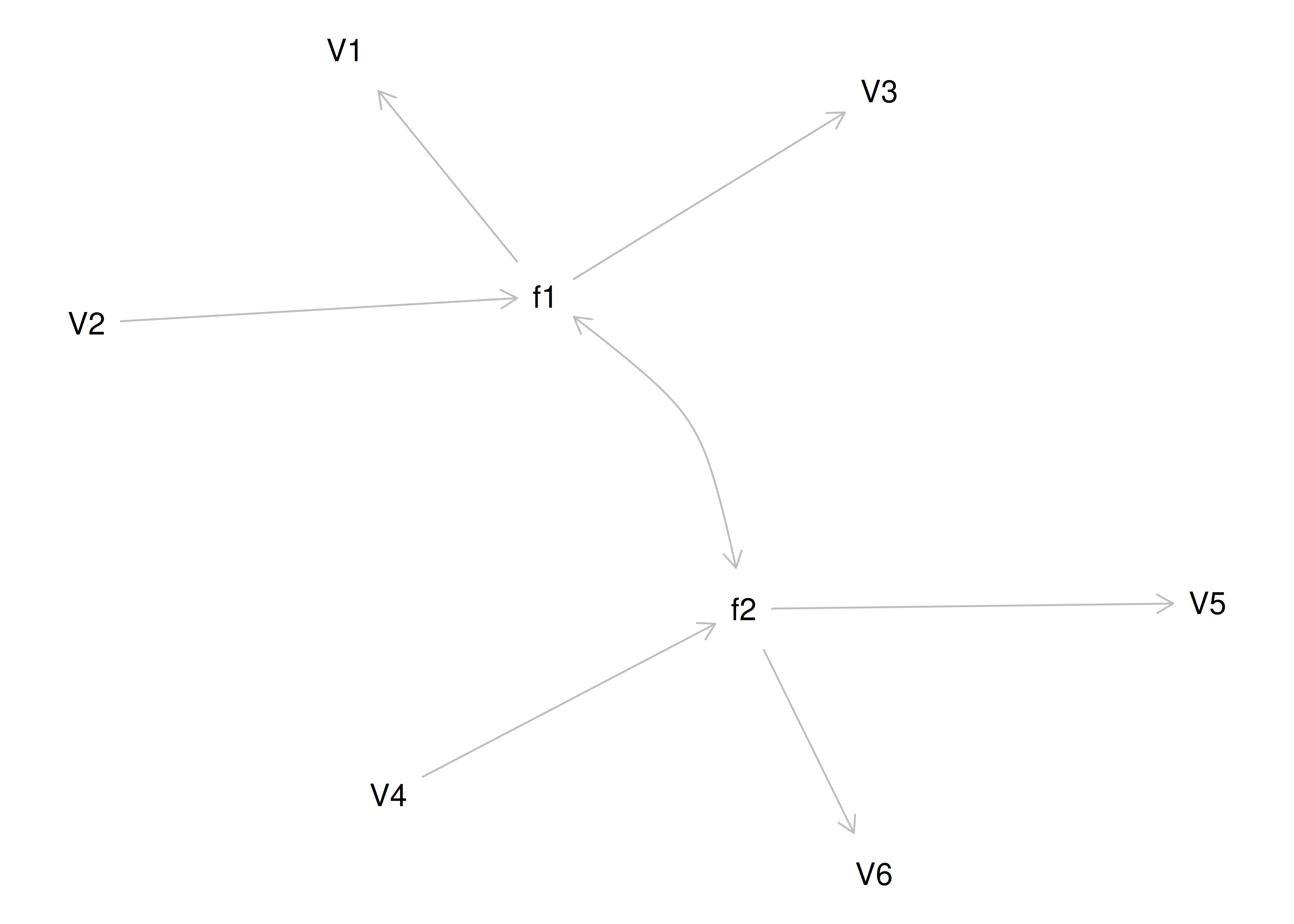
Figure 14.69: Equivalently Fitting Models to Confirmatory Factor Analysis Model 4.
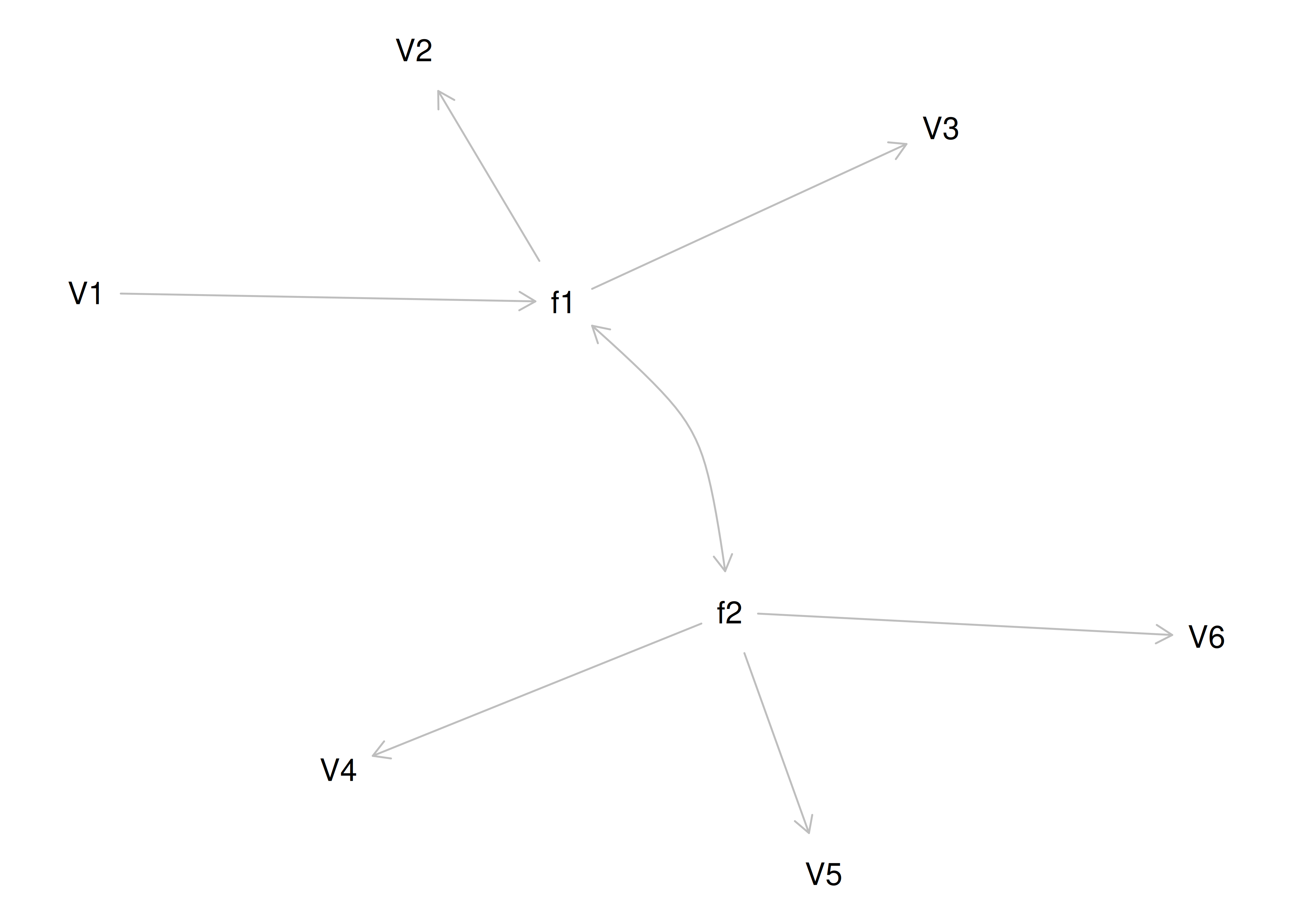
Figure 14.70: Equivalently Fitting Models to Confirmatory Factor Analysis Model 4.
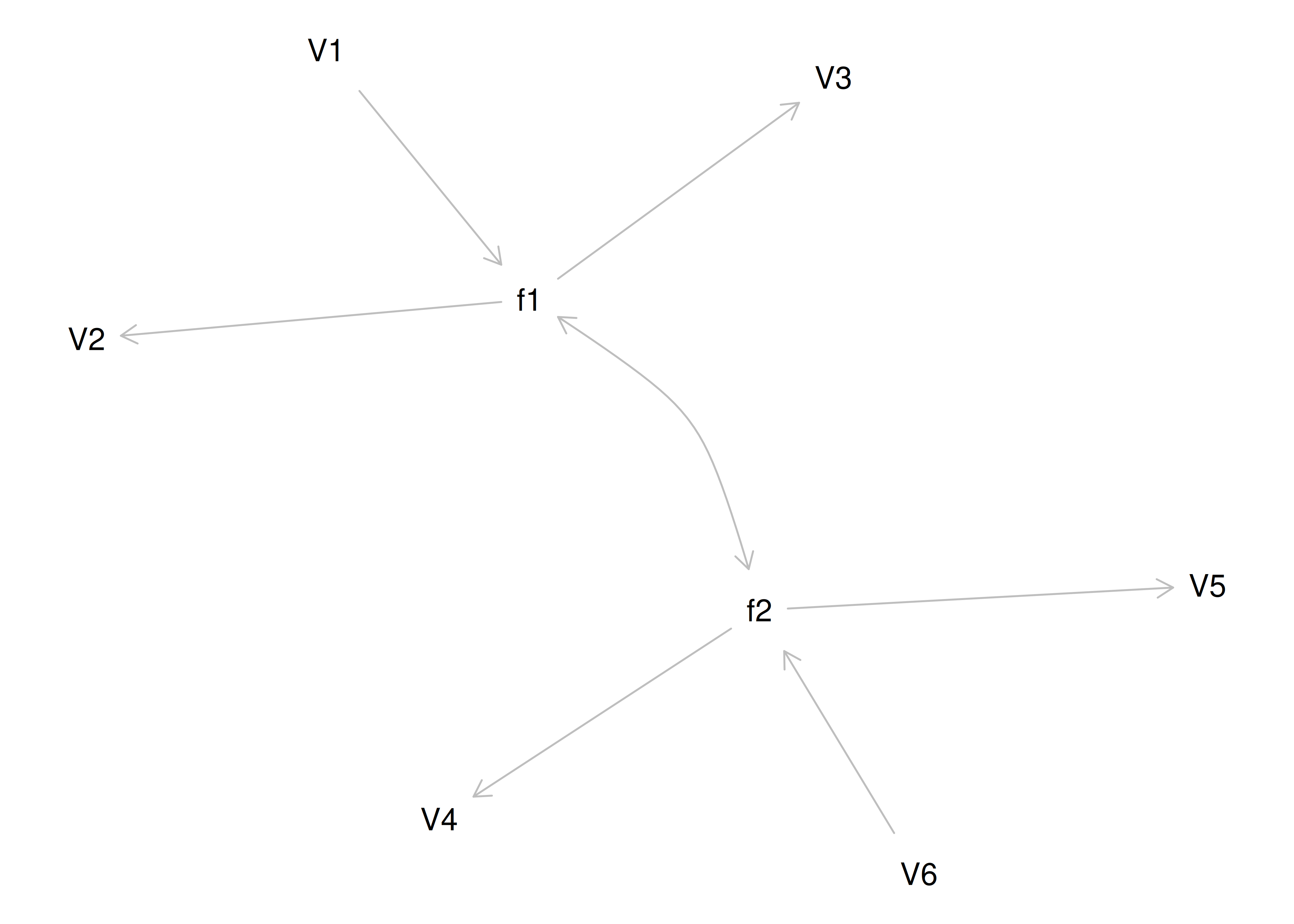
Figure 14.71: Equivalently Fitting Models to Confirmatory Factor Analysis Model 4.
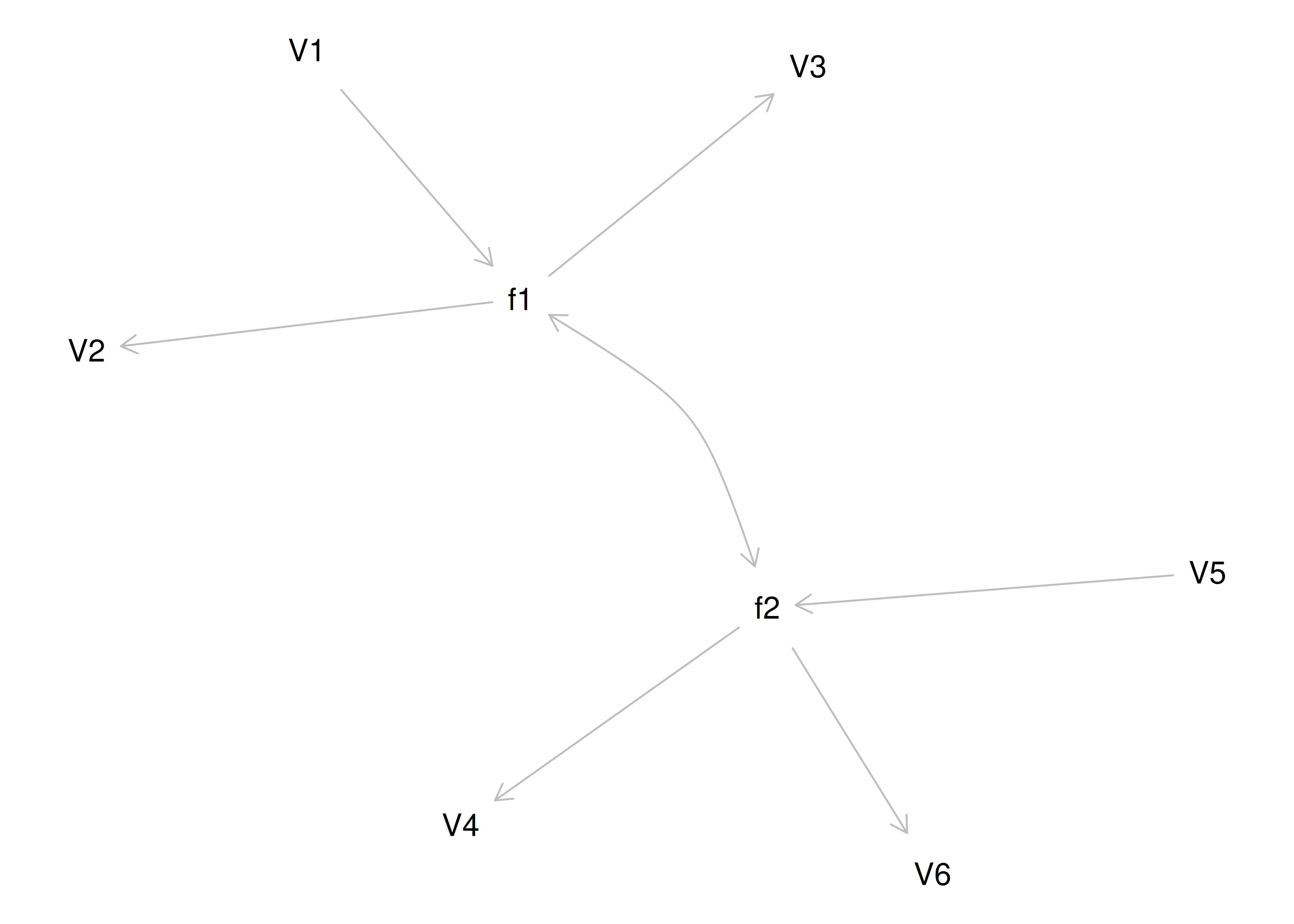
Figure 14.72: Equivalently Fitting Models to Confirmatory Factor Analysis Model 4.
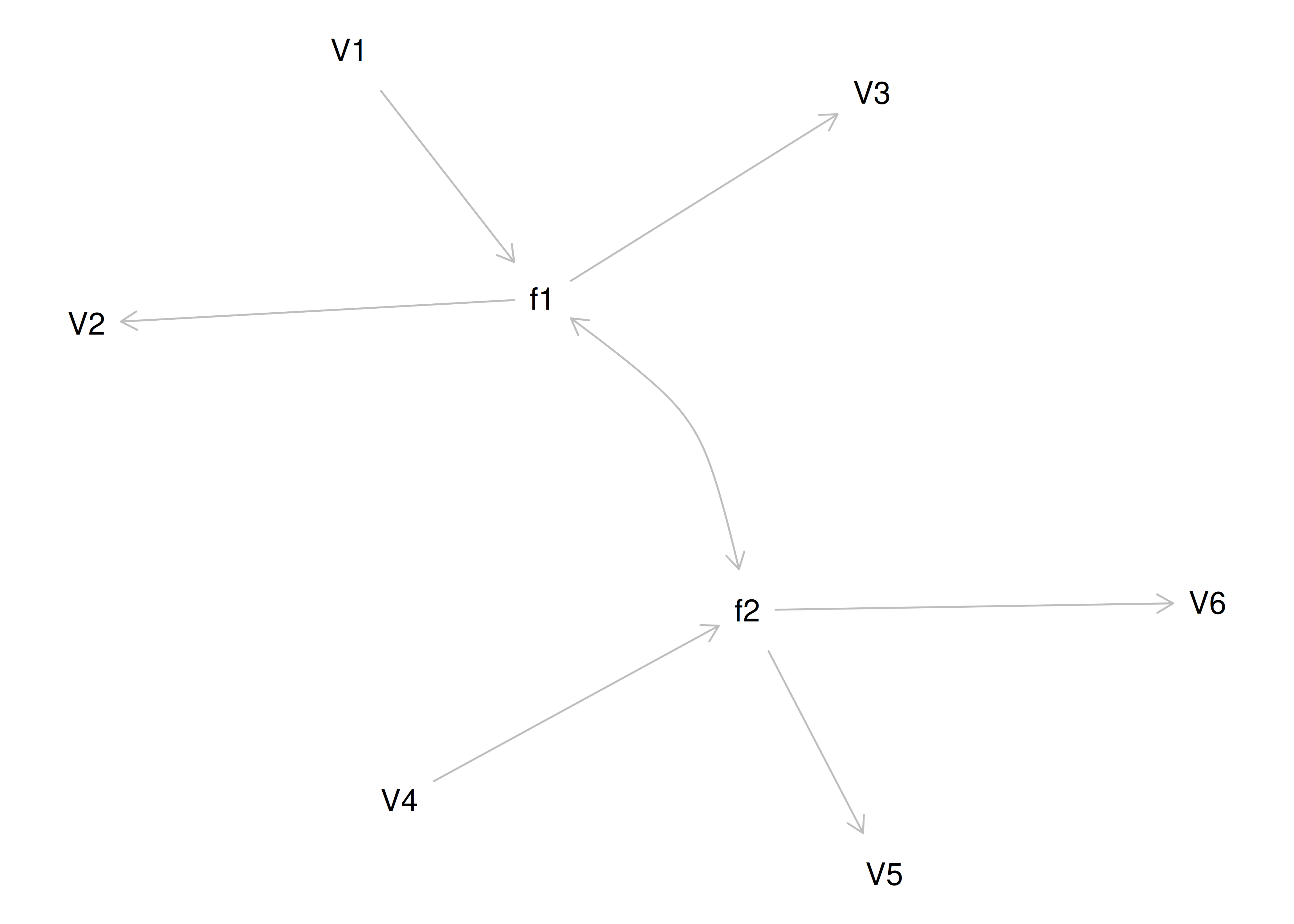
Figure 14.73: Equivalently Fitting Models to Confirmatory Factor Analysis Model 4.
[[1]]
[[1]]$mar
[1] 0 0 0 0
[[2]]
[[2]]$mar
[1] 0 0 0 0
[[3]]
[[3]]$mar
[1] 0 0 0 0
[[4]]
[[4]]$mar
[1] 0 0 0 0
[[5]]
[[5]]$mar
[1] 0 0 0 0
[[6]]
[[6]]$mar
[1] 0 0 0 0
[[7]]
[[7]]$mar
[1] 0 0 0 0
[[8]]
[[8]]$mar
[1] 0 0 0 0
[[9]]
[[9]]$mar
[1] 0 0 0 0
[[10]]
[[10]]$mar
[1] 0 0 0 0
[[11]]
[[11]]$mar
[1] 0 0 0 0
[[12]]
[[12]]$mar
[1] 0 0 0 0
[[13]]
[[13]]$mar
[1] 0 0 0 0
[[14]]
[[14]]$mar
[1] 0 0 0 0
[[15]]
[[15]]$mar
[1] 0 0 0 0
[[16]]
[[16]]$mar
[1] 0 0 0 014.4.2.11 Higher-Order Factor Model
A higher-order (or hierarchical) factor model is a model in which a higher-order latent factor is thought to influence lower-order latent factors. Higher-order factor models are depicted in Figures 14.10 and 14.55. An analysis example of a higher-order factor model is provided in Section 14.4.2.10.4.
14.4.2.12 Bifactor Model
A bifactor model is a model in which both a general latent factor and specific latent factors are extracted from items (Markon, 2019). The general factor represents the common variance among all items, whereas the specific factor represents the common variance among the specific items that load on the specific factor, after extracting the general factor variance. As estimated below, the general factor is orthogonal to the specific factors. Some modified versions of the bifactor allow the specific factors to inter-correlate (in addition to estimating the general factor).
14.4.2.12.1 Specify the model
Code
cfaModelBifactor_syntax <- '
Verbal =~
VO1 + VO2 + VO3 +
VW1 + VW2 + VW3 +
VM1 + VM2 + VM3
Spatial =~
SO1 + SO2 + SO3 +
SW1 + SW2 + SW3 +
SM1 + SM2 + SM3
Quant =~
QO1 + QO2 + QO3 +
QW1 + QW2 + QW3 +
QM1 + QM2 + QM3
g =~
VO1 + VO2 + VO3 +
VW1 + VW2 + VW3 +
VM1 + VM2 + VM3 +
SO1 + SO2 + SO3 +
SW1 + SW2 + SW3 +
SM1 + SM2 + SM3 +
QO1 + QO2 + QO3 +
QW1 + QW2 + QW3 +
QM1 + QM2 + QM3
'
cfaModelBifactor_fullSyntax <- '
#Factor loadings (free the factor loading of the first indicator)
Verbal =~
NA*VO1 + VO2 + VO3 +
VW1 + VW2 + VW3 +
VM1 + VM2 + VM3
Spatial =~
NA*SO1 + SO2 + SO3 +
SW1 + SW2 + SW3 +
SM1 + SM2 + SM3
Quant =~
NA*QO1 + QO2 + QO3 +
QW1 + QW2 + QW3 +
QM1 + QM2 + QM3
g =~
NA*VO1 + VO2 + VO3 +
VW1 + VW2 + VW3 +
VM1 + VM2 + VM3 +
SO1 + SO2 + SO3 +
SW1 + SW2 + SW3 +
SM1 + SM2 + SM3 +
QO1 + QO2 + QO3 +
QW1 + QW2 + QW3 +
QM1 + QM2 + QM3
#Fix latent means to zero
Verbal ~ 0
Spatial ~ 0
Quant ~ 0
g ~ 0
#Fix latent variances to one
Verbal ~~ 1*Verbal
Spatial ~~ 1*Spatial
Quant ~~ 1*Quant
g ~~ 1*g
#Fix covariances among latent variables at zero
Verbal ~~ 0*Spatial
Verbal ~~ 0*Quant
Spatial ~~ 0*Quant
g ~~ 0*Verbal
g ~~ 0*Spatial
g ~~ 0*Quant
#Estimate residual variances of manifest variables
VO1 ~~ VO1
VO2 ~~ VO2
VO3 ~~ VO3
VW1 ~~ VW1
VW2 ~~ VW2
VW3 ~~ VW3
VM1 ~~ VM1
VM2 ~~ VM2
VM3 ~~ VM3
SO1 ~~ SO1
SO2 ~~ SO2
SO3 ~~ SO3
SW1 ~~ SW1
SW2 ~~ SW2
SW3 ~~ SW3
SM1 ~~ SM1
SM2 ~~ SM2
SM3 ~~ SM3
QO1 ~~ QO1
QO2 ~~ QO2
QO3 ~~ QO3
QW1 ~~ QW1
QW2 ~~ QW2
QW3 ~~ QW3
QM1 ~~ QM1
QM2 ~~ QM2
QM3 ~~ QM3
#Free intercepts of manifest variables
VO1 ~ intVO1*1
VO2 ~ intVO2*1
VO3 ~ intVO3*1
VW1 ~ intVW1*1
VW2 ~ intVW2*1
VW3 ~ intVW3*1
VM1 ~ intVM1*1
VM2 ~ intVM2*1
VM3 ~ intVM3*1
SO1 ~ intSO1*1
SO2 ~ intSO2*1
SO3 ~ intSO3*1
SW1 ~ intSW1*1
SW2 ~ intSW2*1
SW3 ~ intSW3*1
SM1 ~ intSM1*1
SM2 ~ intSM2*1
SM3 ~ intSM3*1
QO1 ~ intQO1*1
QO2 ~ intQO2*1
QO3 ~ intQO3*1
QW1 ~ intQW1*1
QW2 ~ intQW2*1
QW3 ~ intQW3*1
QM1 ~ intQM1*1
QM2 ~ intQM2*1
QM3 ~ intQM3*1
'14.4.2.12.3 Fit the model
We simulated the data for the bifactor model in Section 5.3.1.4.2.3.
14.4.2.12.4 Display summary output
lavaan 0.6-20 ended normally after 45 iterations
Estimator ML
Optimization method NLMINB
Number of model parameters 108
Number of observations 10000
Number of missing patterns 1
Model Test User Model:
Standard Scaled
Test Statistic 28930.049 29784.763
Degrees of freedom 297 297
P-value (Chi-square) 0.000 0.000
Scaling correction factor 0.971
Yuan-Bentler correction (Mplus variant)
Model Test Baseline Model:
Test statistic 146391.496 146201.022
Degrees of freedom 351 351
P-value 0.000 0.000
Scaling correction factor 1.001
User Model versus Baseline Model:
Comparative Fit Index (CFI) 0.804 0.798
Tucker-Lewis Index (TLI) 0.768 0.761
Robust Comparative Fit Index (CFI) 0.804
Robust Tucker-Lewis Index (TLI) 0.768
Loglikelihood and Information Criteria:
Loglikelihood user model (H0) -324368.770 -324368.770
Scaling correction factor 1.083
for the MLR correction
Loglikelihood unrestricted model (H1) -309903.745 -309903.745
Scaling correction factor 1.001
for the MLR correction
Akaike (AIC) 648953.539 648953.539
Bayesian (BIC) 649732.256 649732.256
Sample-size adjusted Bayesian (SABIC) 649389.048 649389.048
Root Mean Square Error of Approximation:
RMSEA 0.098 0.100
90 Percent confidence interval - lower 0.097 0.099
90 Percent confidence interval - upper 0.099 0.101
P-value H_0: RMSEA <= 0.050 0.000 0.000
P-value H_0: RMSEA >= 0.080 1.000 1.000
Robust RMSEA 0.098
90 Percent confidence interval - lower 0.097
90 Percent confidence interval - upper 0.099
P-value H_0: Robust RMSEA <= 0.050 0.000
P-value H_0: Robust RMSEA >= 0.080 1.000
Standardized Root Mean Square Residual:
SRMR 0.201 0.201
Parameter Estimates:
Standard errors Sandwich
Information bread Observed
Observed information based on Hessian
Latent Variables:
Estimate Std.Err z-value P(>|z|) Std.lv Std.all
Verbal =~
VO1 0.484 0.011 42.953 0.000 0.484 0.484
VO2 0.572 0.012 49.110 0.000 0.572 0.571
VO3 0.648 0.011 59.594 0.000 0.648 0.649
VW1 0.602 0.021 28.399 0.000 0.602 0.597
VW2 0.522 0.017 31.037 0.000 0.522 0.516
VW3 0.457 0.015 31.401 0.000 0.457 0.452
VM1 0.764 0.009 81.260 0.000 0.764 0.758
VM2 0.837 0.009 91.851 0.000 0.837 0.835
VM3 0.574 0.010 58.967 0.000 0.574 0.576
Spatial =~
SO1 0.597 0.011 52.050 0.000 0.597 0.603
SO2 0.603 0.012 51.513 0.000 0.603 0.603
SO3 0.530 0.012 45.701 0.000 0.530 0.531
SW1 0.491 0.021 23.493 0.000 0.491 0.489
SW2 0.584 0.020 29.673 0.000 0.584 0.584
SW3 0.416 0.018 22.716 0.000 0.416 0.417
SM1 0.856 0.008 103.159 0.000 0.856 0.860
SM2 0.682 0.009 72.543 0.000 0.682 0.684
SM3 0.892 0.008 106.899 0.000 0.892 0.895
Quant =~
QO1 0.532 0.011 46.627 0.000 0.532 0.537
QO2 0.673 0.010 67.359 0.000 0.673 0.680
QO3 0.529 0.011 47.899 0.000 0.529 0.526
QW1 0.454 0.014 33.332 0.000 0.454 0.452
QW2 0.526 0.013 39.384 0.000 0.526 0.533
QW3 0.616 0.015 40.075 0.000 0.616 0.618
QM1 0.595 0.010 57.570 0.000 0.595 0.596
QM2 0.652 0.010 64.766 0.000 0.652 0.648
QM3 0.743 0.010 75.444 0.000 0.743 0.740
g =~
VO1 -0.116 0.020 -5.713 0.000 -0.116 -0.116
VO2 -0.155 0.023 -6.756 0.000 -0.155 -0.155
VO3 -0.181 0.024 -7.540 0.000 -0.181 -0.181
VW1 -0.699 0.021 -32.569 0.000 -0.699 -0.693
VW2 -0.514 0.020 -26.246 0.000 -0.514 -0.508
VW3 -0.397 0.018 -21.773 0.000 -0.397 -0.393
VM1 0.038 0.030 1.237 0.216 0.038 0.037
VM2 0.013 0.033 0.407 0.684 0.013 0.013
VM3 -0.013 0.023 -0.552 0.581 -0.013 -0.013
SO1 -0.202 0.023 -8.812 0.000 -0.202 -0.204
SO2 -0.208 0.023 -8.965 0.000 -0.208 -0.208
SO3 -0.153 0.023 -6.818 0.000 -0.153 -0.154
SW1 -0.684 0.018 -37.922 0.000 -0.684 -0.682
SW2 -0.633 0.021 -30.390 0.000 -0.633 -0.633
SW3 -0.563 0.016 -34.126 0.000 -0.563 -0.565
SM1 -0.010 0.031 -0.318 0.751 -0.010 -0.010
SM2 0.070 0.027 2.618 0.009 0.070 0.070
SM3 0.027 0.034 0.789 0.430 0.027 0.027
QO1 -0.088 0.019 -4.585 0.000 -0.088 -0.089
QO2 -0.133 0.020 -6.651 0.000 -0.133 -0.134
QO3 -0.090 0.018 -5.060 0.000 -0.090 -0.090
QW1 -0.452 0.015 -30.307 0.000 -0.452 -0.449
QW2 -0.461 0.016 -27.995 0.000 -0.461 -0.467
QW3 -0.574 0.018 -32.789 0.000 -0.574 -0.576
QM1 0.060 0.024 2.504 0.012 0.060 0.060
QM2 -0.000 0.023 -0.020 0.984 -0.000 -0.000
QM3 -0.040 0.026 -1.567 0.117 -0.040 -0.040
Covariances:
Estimate Std.Err z-value P(>|z|) Std.lv Std.all
Verbal ~~
Spatial 0.000 0.000 0.000
Quant 0.000 0.000 0.000
g 0.000 0.000 0.000
Spatial ~~
Quant 0.000 0.000 0.000
g 0.000 0.000 0.000
Quant ~~
g 0.000 0.000 0.000
Intercepts:
Estimate Std.Err z-value P(>|z|) Std.lv Std.all
.VO1 -0.007 0.010 -0.717 0.473 -0.007 -0.007
.VO2 -0.013 0.010 -1.254 0.210 -0.013 -0.013
.VO3 -0.008 0.010 -0.815 0.415 -0.008 -0.008
.VW1 0.015 0.010 1.464 0.143 0.015 0.015
.VW2 0.011 0.010 1.043 0.297 0.011 0.010
.VW3 -0.006 0.010 -0.572 0.567 -0.006 -0.006
.VM1 -0.011 0.010 -1.086 0.277 -0.011 -0.011
.VM2 -0.010 0.010 -0.992 0.321 -0.010 -0.010
.VM3 -0.012 0.010 -1.195 0.232 -0.012 -0.012
.SO1 -0.006 0.010 -0.588 0.557 -0.006 -0.006
.SO2 -0.014 0.010 -1.405 0.160 -0.014 -0.014
.SO3 -0.008 0.010 -0.827 0.408 -0.008 -0.008
.SW1 0.004 0.010 0.405 0.686 0.004 0.004
.SW2 0.007 0.010 0.673 0.501 0.007 0.007
.SW3 0.005 0.010 0.472 0.637 0.005 0.005
.SM1 -0.009 0.010 -0.913 0.361 -0.009 -0.009
.SM2 -0.008 0.010 -0.754 0.451 -0.008 -0.008
.SM3 -0.012 0.010 -1.185 0.236 -0.012 -0.012
.QO1 0.005 0.010 0.479 0.632 0.005 0.005
.QO2 0.005 0.010 0.458 0.647 0.005 0.005
.QO3 -0.001 0.010 -0.144 0.886 -0.001 -0.001
.QW1 0.010 0.010 0.950 0.342 0.010 0.009
.QW2 0.013 0.010 1.268 0.205 0.013 0.013
.QW3 0.025 0.010 2.555 0.011 0.025 0.026
.QM1 -0.000 0.010 -0.046 0.963 -0.000 -0.000
.QM2 0.009 0.010 0.876 0.381 0.009 0.009
.QM3 0.004 0.010 0.379 0.704 0.004 0.004
Variances:
Estimate Std.Err z-value P(>|z|) Std.lv Std.all
.VO1 0.754 0.012 64.731 0.000 0.754 0.752
.VO2 0.652 0.010 62.803 0.000 0.652 0.650
.VO3 0.544 0.009 58.899 0.000 0.544 0.546
.VW1 0.166 0.005 34.098 0.000 0.166 0.163
.VW2 0.486 0.007 64.831 0.000 0.486 0.475
.VW3 0.656 0.010 68.200 0.000 0.656 0.642
.VM1 0.431 0.009 49.752 0.000 0.431 0.425
.VM2 0.303 0.008 37.128 0.000 0.303 0.302
.VM3 0.663 0.010 65.608 0.000 0.663 0.668
.SO1 0.581 0.009 66.646 0.000 0.581 0.594
.SO2 0.592 0.009 66.143 0.000 0.592 0.593
.SO3 0.692 0.010 67.404 0.000 0.692 0.695
.SW1 0.297 0.006 52.133 0.000 0.297 0.295
.SW2 0.259 0.005 52.718 0.000 0.259 0.259
.SW3 0.503 0.008 65.638 0.000 0.503 0.507
.SM1 0.258 0.005 49.904 0.000 0.258 0.260
.SM2 0.525 0.008 63.106 0.000 0.525 0.527
.SM3 0.198 0.006 34.081 0.000 0.198 0.199
.QO1 0.691 0.011 60.174 0.000 0.691 0.704
.QO2 0.510 0.009 54.337 0.000 0.510 0.520
.QO3 0.723 0.012 62.650 0.000 0.723 0.715
.QW1 0.600 0.009 64.160 0.000 0.600 0.594
.QW2 0.486 0.008 61.850 0.000 0.486 0.498
.QW3 0.285 0.006 46.027 0.000 0.285 0.286
.QM1 0.638 0.011 58.684 0.000 0.638 0.641
.QM2 0.586 0.010 59.577 0.000 0.586 0.580
.QM3 0.454 0.009 50.592 0.000 0.454 0.451
Verbal 1.000 1.000 1.000
Spatial 1.000 1.000 1.000
Quant 1.000 1.000 1.000
g 1.000 1.000 1.000
R-Square:
Estimate
VO1 0.248
VO2 0.350
VO3 0.454
VW1 0.837
VW2 0.525
VW3 0.358
VM1 0.575
VM2 0.698
VM3 0.332
SO1 0.406
SO2 0.407
SO3 0.305
SW1 0.705
SW2 0.741
SW3 0.493
SM1 0.740
SM2 0.473
SM3 0.801
QO1 0.296
QO2 0.480
QO3 0.285
QW1 0.406
QW2 0.502
QW3 0.714
QM1 0.359
QM2 0.420
QM3 0.549lavaan 0.6-20 ended normally after 45 iterations
Estimator ML
Optimization method NLMINB
Number of model parameters 108
Number of observations 10000
Number of missing patterns 1
Model Test User Model:
Standard Scaled
Test Statistic 28930.049 29784.763
Degrees of freedom 297 297
P-value (Chi-square) 0.000 0.000
Scaling correction factor 0.971
Yuan-Bentler correction (Mplus variant)
Model Test Baseline Model:
Test statistic 146391.496 146201.022
Degrees of freedom 351 351
P-value 0.000 0.000
Scaling correction factor 1.001
User Model versus Baseline Model:
Comparative Fit Index (CFI) 0.804 0.798
Tucker-Lewis Index (TLI) 0.768 0.761
Robust Comparative Fit Index (CFI) 0.804
Robust Tucker-Lewis Index (TLI) 0.768
Loglikelihood and Information Criteria:
Loglikelihood user model (H0) -324368.770 -324368.770
Scaling correction factor 1.083
for the MLR correction
Loglikelihood unrestricted model (H1) -309903.745 -309903.745
Scaling correction factor 1.001
for the MLR correction
Akaike (AIC) 648953.539 648953.539
Bayesian (BIC) 649732.256 649732.256
Sample-size adjusted Bayesian (SABIC) 649389.048 649389.048
Root Mean Square Error of Approximation:
RMSEA 0.098 0.100
90 Percent confidence interval - lower 0.097 0.099
90 Percent confidence interval - upper 0.099 0.101
P-value H_0: RMSEA <= 0.050 0.000 0.000
P-value H_0: RMSEA >= 0.080 1.000 1.000
Robust RMSEA 0.098
90 Percent confidence interval - lower 0.097
90 Percent confidence interval - upper 0.099
P-value H_0: Robust RMSEA <= 0.050 0.000
P-value H_0: Robust RMSEA >= 0.080 1.000
Standardized Root Mean Square Residual:
SRMR 0.201 0.201
Parameter Estimates:
Standard errors Sandwich
Information bread Observed
Observed information based on Hessian
Latent Variables:
Estimate Std.Err z-value P(>|z|) Std.lv Std.all
Verbal =~
VO1 0.484 0.011 42.953 0.000 0.484 0.484
VO2 0.572 0.012 49.110 0.000 0.572 0.571
VO3 0.648 0.011 59.594 0.000 0.648 0.649
VW1 0.602 0.021 28.399 0.000 0.602 0.597
VW2 0.522 0.017 31.037 0.000 0.522 0.516
VW3 0.457 0.015 31.401 0.000 0.457 0.452
VM1 0.764 0.009 81.260 0.000 0.764 0.758
VM2 0.837 0.009 91.851 0.000 0.837 0.835
VM3 0.574 0.010 58.967 0.000 0.574 0.576
Spatial =~
SO1 0.597 0.011 52.050 0.000 0.597 0.603
SO2 0.603 0.012 51.513 0.000 0.603 0.603
SO3 0.530 0.012 45.701 0.000 0.530 0.531
SW1 0.491 0.021 23.493 0.000 0.491 0.489
SW2 0.584 0.020 29.673 0.000 0.584 0.584
SW3 0.416 0.018 22.716 0.000 0.416 0.417
SM1 0.856 0.008 103.159 0.000 0.856 0.860
SM2 0.682 0.009 72.543 0.000 0.682 0.684
SM3 0.892 0.008 106.899 0.000 0.892 0.895
Quant =~
QO1 0.532 0.011 46.627 0.000 0.532 0.537
QO2 0.673 0.010 67.359 0.000 0.673 0.680
QO3 0.529 0.011 47.899 0.000 0.529 0.526
QW1 0.454 0.014 33.332 0.000 0.454 0.452
QW2 0.526 0.013 39.384 0.000 0.526 0.533
QW3 0.616 0.015 40.075 0.000 0.616 0.618
QM1 0.595 0.010 57.570 0.000 0.595 0.596
QM2 0.652 0.010 64.766 0.000 0.652 0.648
QM3 0.743 0.010 75.444 0.000 0.743 0.740
g =~
VO1 -0.116 0.020 -5.713 0.000 -0.116 -0.116
VO2 -0.155 0.023 -6.756 0.000 -0.155 -0.155
VO3 -0.181 0.024 -7.540 0.000 -0.181 -0.181
VW1 -0.699 0.021 -32.569 0.000 -0.699 -0.693
VW2 -0.514 0.020 -26.246 0.000 -0.514 -0.508
VW3 -0.397 0.018 -21.773 0.000 -0.397 -0.393
VM1 0.038 0.030 1.237 0.216 0.038 0.037
VM2 0.013 0.033 0.407 0.684 0.013 0.013
VM3 -0.013 0.023 -0.552 0.581 -0.013 -0.013
SO1 -0.202 0.023 -8.812 0.000 -0.202 -0.204
SO2 -0.208 0.023 -8.965 0.000 -0.208 -0.208
SO3 -0.153 0.023 -6.818 0.000 -0.153 -0.154
SW1 -0.684 0.018 -37.922 0.000 -0.684 -0.682
SW2 -0.633 0.021 -30.390 0.000 -0.633 -0.633
SW3 -0.563 0.016 -34.126 0.000 -0.563 -0.565
SM1 -0.010 0.031 -0.318 0.751 -0.010 -0.010
SM2 0.070 0.027 2.618 0.009 0.070 0.070
SM3 0.027 0.034 0.789 0.430 0.027 0.027
QO1 -0.088 0.019 -4.585 0.000 -0.088 -0.089
QO2 -0.133 0.020 -6.651 0.000 -0.133 -0.134
QO3 -0.090 0.018 -5.060 0.000 -0.090 -0.090
QW1 -0.452 0.015 -30.307 0.000 -0.452 -0.449
QW2 -0.461 0.016 -27.995 0.000 -0.461 -0.467
QW3 -0.574 0.018 -32.789 0.000 -0.574 -0.576
QM1 0.060 0.024 2.504 0.012 0.060 0.060
QM2 -0.000 0.023 -0.020 0.984 -0.000 -0.000
QM3 -0.040 0.026 -1.567 0.117 -0.040 -0.040
Covariances:
Estimate Std.Err z-value P(>|z|) Std.lv Std.all
Verbal ~~
Spatial 0.000 0.000 0.000
Quant 0.000 0.000 0.000
Spatial ~~
Quant 0.000 0.000 0.000
Verbal ~~
g 0.000 0.000 0.000
Spatial ~~
g 0.000 0.000 0.000
Quant ~~
g 0.000 0.000 0.000
Intercepts:
Estimate Std.Err z-value P(>|z|) Std.lv Std.all
Verbal 0.000 0.000 0.000
Spatial 0.000 0.000 0.000
Quant 0.000 0.000 0.000
g 0.000 0.000 0.000
.VO1 (iVO1) -0.007 0.010 -0.717 0.473 -0.007 -0.007
.VO2 (iVO2) -0.013 0.010 -1.254 0.210 -0.013 -0.013
.VO3 (iVO3) -0.008 0.010 -0.815 0.415 -0.008 -0.008
.VW1 (iVW1) 0.015 0.010 1.464 0.143 0.015 0.015
.VW2 (iVW2) 0.011 0.010 1.043 0.297 0.011 0.010
.VW3 (iVW3) -0.006 0.010 -0.572 0.567 -0.006 -0.006
.VM1 (iVM1) -0.011 0.010 -1.086 0.277 -0.011 -0.011
.VM2 (iVM2) -0.010 0.010 -0.992 0.321 -0.010 -0.010
.VM3 (iVM3) -0.012 0.010 -1.195 0.232 -0.012 -0.012
.SO1 (iSO1) -0.006 0.010 -0.588 0.557 -0.006 -0.006
.SO2 (iSO2) -0.014 0.010 -1.405 0.160 -0.014 -0.014
.SO3 (iSO3) -0.008 0.010 -0.827 0.408 -0.008 -0.008
.SW1 (iSW1) 0.004 0.010 0.405 0.686 0.004 0.004
.SW2 (iSW2) 0.007 0.010 0.673 0.501 0.007 0.007
.SW3 (iSW3) 0.005 0.010 0.472 0.637 0.005 0.005
.SM1 (iSM1) -0.009 0.010 -0.913 0.361 -0.009 -0.009
.SM2 (iSM2) -0.008 0.010 -0.754 0.451 -0.008 -0.008
.SM3 (iSM3) -0.012 0.010 -1.185 0.236 -0.012 -0.012
.QO1 (iQO1) 0.005 0.010 0.479 0.632 0.005 0.005
.QO2 (iQO2) 0.005 0.010 0.458 0.647 0.005 0.005
.QO3 (iQO3) -0.001 0.010 -0.144 0.886 -0.001 -0.001
.QW1 (iQW1) 0.010 0.010 0.950 0.342 0.010 0.009
.QW2 (iQW2) 0.013 0.010 1.268 0.205 0.013 0.013
.QW3 (iQW3) 0.025 0.010 2.555 0.011 0.025 0.026
.QM1 (iQM1) -0.000 0.010 -0.046 0.963 -0.000 -0.000
.QM2 (iQM2) 0.009 0.010 0.876 0.381 0.009 0.009
.QM3 (iQM3) 0.004 0.010 0.379 0.704 0.004 0.004
Variances:
Estimate Std.Err z-value P(>|z|) Std.lv Std.all
Verbal 1.000 1.000 1.000
Spatial 1.000 1.000 1.000
Quant 1.000 1.000 1.000
g 1.000 1.000 1.000
.VO1 0.754 0.012 64.731 0.000 0.754 0.752
.VO2 0.652 0.010 62.803 0.000 0.652 0.650
.VO3 0.544 0.009 58.899 0.000 0.544 0.546
.VW1 0.166 0.005 34.098 0.000 0.166 0.163
.VW2 0.486 0.007 64.831 0.000 0.486 0.475
.VW3 0.656 0.010 68.200 0.000 0.656 0.642
.VM1 0.431 0.009 49.752 0.000 0.431 0.425
.VM2 0.303 0.008 37.128 0.000 0.303 0.302
.VM3 0.663 0.010 65.608 0.000 0.663 0.668
.SO1 0.581 0.009 66.646 0.000 0.581 0.594
.SO2 0.592 0.009 66.143 0.000 0.592 0.593
.SO3 0.692 0.010 67.404 0.000 0.692 0.695
.SW1 0.297 0.006 52.133 0.000 0.297 0.295
.SW2 0.259 0.005 52.718 0.000 0.259 0.259
.SW3 0.503 0.008 65.638 0.000 0.503 0.507
.SM1 0.258 0.005 49.904 0.000 0.258 0.260
.SM2 0.525 0.008 63.106 0.000 0.525 0.527
.SM3 0.198 0.006 34.081 0.000 0.198 0.199
.QO1 0.691 0.011 60.174 0.000 0.691 0.704
.QO2 0.510 0.009 54.337 0.000 0.510 0.520
.QO3 0.723 0.012 62.650 0.000 0.723 0.715
.QW1 0.600 0.009 64.160 0.000 0.600 0.594
.QW2 0.486 0.008 61.850 0.000 0.486 0.498
.QW3 0.285 0.006 46.027 0.000 0.285 0.286
.QM1 0.638 0.011 58.684 0.000 0.638 0.641
.QM2 0.586 0.010 59.577 0.000 0.586 0.580
.QM3 0.454 0.009 50.592 0.000 0.454 0.451
R-Square:
Estimate
VO1 0.248
VO2 0.350
VO3 0.454
VW1 0.837
VW2 0.525
VW3 0.358
VM1 0.575
VM2 0.698
VM3 0.332
SO1 0.406
SO2 0.407
SO3 0.305
SW1 0.705
SW2 0.741
SW3 0.493
SM1 0.740
SM2 0.473
SM3 0.801
QO1 0.296
QO2 0.480
QO3 0.285
QW1 0.406
QW2 0.502
QW3 0.714
QM1 0.359
QM2 0.420
QM3 0.54914.4.2.12.5 Estimates of model fit
Code
chisq df pvalue
28930.049 297.000 0.000
chisq.scaled df.scaled pvalue.scaled
29784.763 297.000 0.000
chisq.scaling.factor baseline.chisq baseline.df
0.971 146391.496 351.000
baseline.pvalue rmsea cfi
0.000 0.098 0.804
tli srmr rmsea.robust
0.768 0.201 0.098
cfi.robust tli.robust
0.804 0.768 14.4.2.12.6 Residuals
$type
[1] "cor.bollen"
$cov
VO1 VO2 VO3 VW1 VW2 VW3 VM1 VM2 VM3 SO1
VO1 0.000
VO2 0.202 0.000
VO3 0.139 0.175 0.000
VW1 -0.022 -0.015 -0.015 0.000
VW2 -0.011 -0.008 0.003 0.004 0.000
VW3 0.001 -0.006 0.006 0.003 0.000 0.000
VM1 -0.057 -0.058 -0.045 0.007 -0.010 0.000 0.000
VM2 -0.045 -0.052 -0.035 0.009 0.004 -0.001 0.039 0.000
VM3 -0.031 -0.026 -0.022 0.001 0.001 -0.011 0.021 0.013 0.000
SO1 0.336 0.408 0.398 0.215 0.197 0.181 0.312 0.345 0.239 0.000
SO2 0.331 0.406 0.393 0.206 0.196 0.183 0.304 0.342 0.237 0.170
SO3 0.401 0.480 0.419 0.187 0.180 0.157 0.257 0.285 0.213 0.214
SW1 0.119 0.146 0.167 0.180 0.153 0.117 0.282 0.299 0.200 -0.016
SW2 0.169 0.194 0.231 0.210 0.181 0.166 0.336 0.358 0.240 0.008
SW3 0.110 0.130 0.145 0.151 0.125 0.108 0.245 0.257 0.172 -0.013
SM1 0.250 0.300 0.356 0.350 0.309 0.253 0.544 0.588 0.389 -0.024
SM2 0.187 0.218 0.274 0.296 0.250 0.211 0.460 0.493 0.325 -0.055
SM3 0.261 0.312 0.366 0.380 0.324 0.280 0.598 0.644 0.422 -0.037
QO1 0.377 0.458 0.376 0.154 0.136 0.126 0.187 0.221 0.150 0.327
QO2 0.306 0.372 0.361 0.190 0.183 0.174 0.255 0.294 0.212 0.303
QO3 0.292 0.360 0.316 0.142 0.123 0.116 0.181 0.209 0.146 0.272
QW1 0.102 0.116 0.141 0.142 0.108 0.107 0.206 0.218 0.154 0.092
QW2 0.113 0.133 0.167 0.166 0.141 0.124 0.242 0.259 0.183 0.115
QW3 0.126 0.154 0.186 0.189 0.154 0.140 0.270 0.297 0.194 0.122
QM1 0.146 0.192 0.234 0.248 0.211 0.191 0.385 0.407 0.266 0.189
QM2 0.170 0.209 0.260 0.247 0.214 0.196 0.369 0.400 0.253 0.203
QM3 0.204 0.249 0.303 0.284 0.238 0.221 0.412 0.455 0.301 0.235
SO2 SO3 SW1 SW2 SW3 SM1 SM2 SM3 QO1 QO2
VO1
VO2
VO3
VW1
VW2
VW3
VM1
VM2
VM3
SO1
SO2 0.000
SO3 0.218 0.000
SW1 -0.010 -0.022 0.000
SW2 0.003 0.004 0.002 0.000
SW3 -0.010 -0.011 0.005 0.004 0.000
SM1 -0.023 -0.036 0.000 -0.003 -0.004 0.000
SM2 -0.058 -0.055 0.005 -0.008 0.011 0.003 0.000
SM3 -0.038 -0.047 0.006 0.000 0.003 0.018 0.032 0.000
QO1 0.328 0.427 0.077 0.112 0.075 0.172 0.124 0.182 0.000
QO2 0.301 0.345 0.099 0.156 0.091 0.240 0.179 0.251 0.155 0.000
QO3 0.267 0.329 0.073 0.111 0.067 0.169 0.122 0.180 0.196 0.104
QW1 0.091 0.081 0.082 0.097 0.069 0.178 0.147 0.194 -0.019 -0.022
QW2 0.115 0.096 0.094 0.125 0.087 0.224 0.182 0.234 -0.040 -0.019
QW3 0.129 0.110 0.111 0.134 0.104 0.241 0.203 0.261 -0.040 -0.021
QM1 0.185 0.167 0.185 0.219 0.170 0.382 0.313 0.416 -0.066 -0.056
QM2 0.206 0.171 0.180 0.203 0.154 0.361 0.296 0.394 -0.047 -0.025
QM3 0.232 0.201 0.182 0.232 0.163 0.392 0.327 0.428 -0.055 -0.020
QO3 QW1 QW2 QW3 QM1 QM2 QM3
VO1
VO2
VO3
VW1
VW2
VW3
VM1
VM2
VM3
SO1
SO2
SO3
SW1
SW2
SW3
SM1
SM2
SM3
QO1
QO2
QO3 0.000
QW1 -0.020 0.000
QW2 -0.029 0.006 0.000
QW3 -0.026 0.014 0.017 0.000
QM1 -0.064 0.016 0.009 0.019 0.000
QM2 -0.047 0.005 0.007 0.011 0.036 0.000
QM3 -0.043 -0.001 0.012 0.012 0.041 0.021 0.000
$mean
VO1 VO2 VO3 VW1 VW2 VW3 VM1 VM2 VM3 SO1 SO2 SO3 SW1 SW2 SW3 SM1 SM2 SM3 QO1 QO2
0 0 0 0 0 0 0 0 0 0 0 0 0 0 0 0 0 0 0 0
QO3 QW1 QW2 QW3 QM1 QM2 QM3
0 0 0 0 0 0 0 14.4.2.12.8 Internal Consistency Reliability
Internal consistency reliability of items composing the latent factors, as quantified by omega (\(\omega\)) and average variance extracted (AVE), was estimated using the semTools package (Jorgensen et al., 2021).
Verbal Spatial Quant g
0.767 0.763 0.776 0.148 Verbal Spatial Quant g
NA NA NA NA 14.4.2.12.9 Bifactor Indices
$ModelLevelIndices
ECV.g PUC Omega.g OmegaH.g
0.2269664 0.6923077 0.9042907 0.2675674
$FactorLevelIndices
ECV_SS ECV_SG ECV_GS Omega OmegaH H FD
Verbal 0.7796232 0.2535731 0.2203768 0.8790893 0.7736569 0.8725556 0.9379034
Spatial 0.7437332 0.2801751 0.2562668 0.9055216 0.7716862 0.9115181 0.9556202
Quant 0.8028779 0.2392854 0.1971221 0.8636425 0.7764942 0.8438576 0.9229303
g 0.2269664 0.2269664 0.2269664 0.9042907 0.2675674 0.8252431 0.9330779
$ItemLevelIndices
IECV
VO1 5.408760e-02
VO2 6.860534e-02
VO3 7.208035e-02
VW1 5.741486e-01
VW2 4.917804e-01
VW3 4.305963e-01
VM1 2.419812e-03
VM2 2.512524e-04
VM3 4.761137e-04
SO1 1.030198e-01
SO2 1.060770e-01
SO3 7.745478e-02
SW1 6.601119e-01
SW2 5.406438e-01
SW3 6.470682e-01
SM1 1.348563e-04
SM2 1.033748e-02
SM3 8.829106e-04
QO1 2.675989e-02
QO2 3.751198e-02
QO3 2.824797e-02
QW1 4.969037e-01
QW2 4.341995e-01
QW3 4.649665e-01
QM1 9.936411e-03
QM2 5.290108e-07
QM3 2.889265e-0314.4.2.12.10 Path diagram
A path diagram of the model generated using the semPlot package (Epskamp, 2022) is in Figure 14.74.
Code
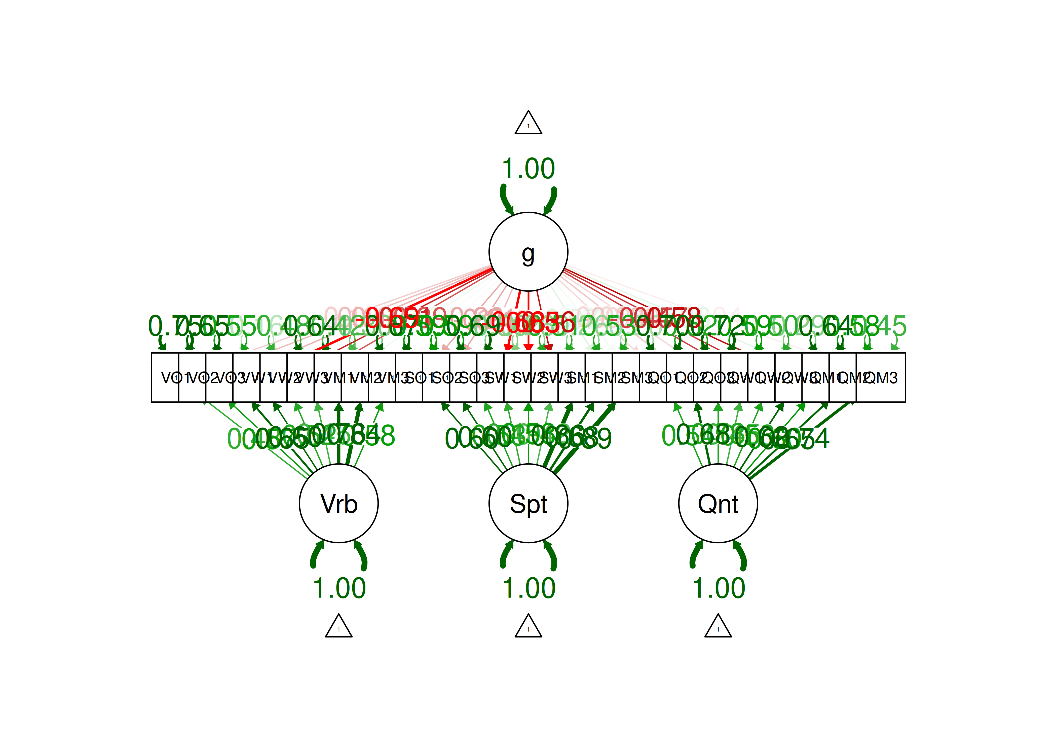
Figure 14.74: Bifactor Model.
14.4.2.12.11 Equivalently fitting models
Markov equivalent directed acyclic graphs (DAGs) were depicted using the dagitty package (Textor et al., 2021).
Path diagrams of equivalent models are below.
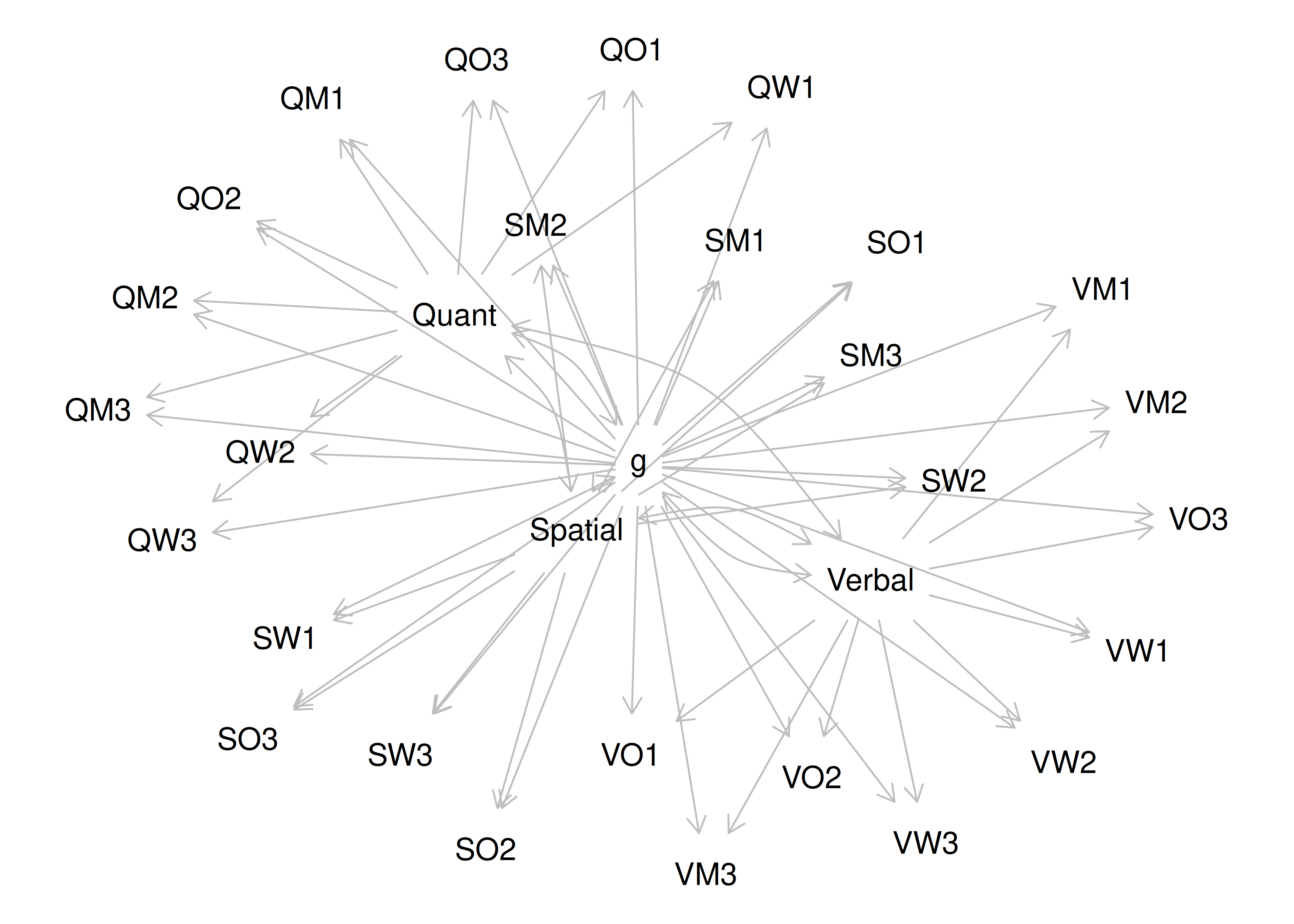
Figure 14.75: Equivalently Fitting Models to a Bifactor Model.
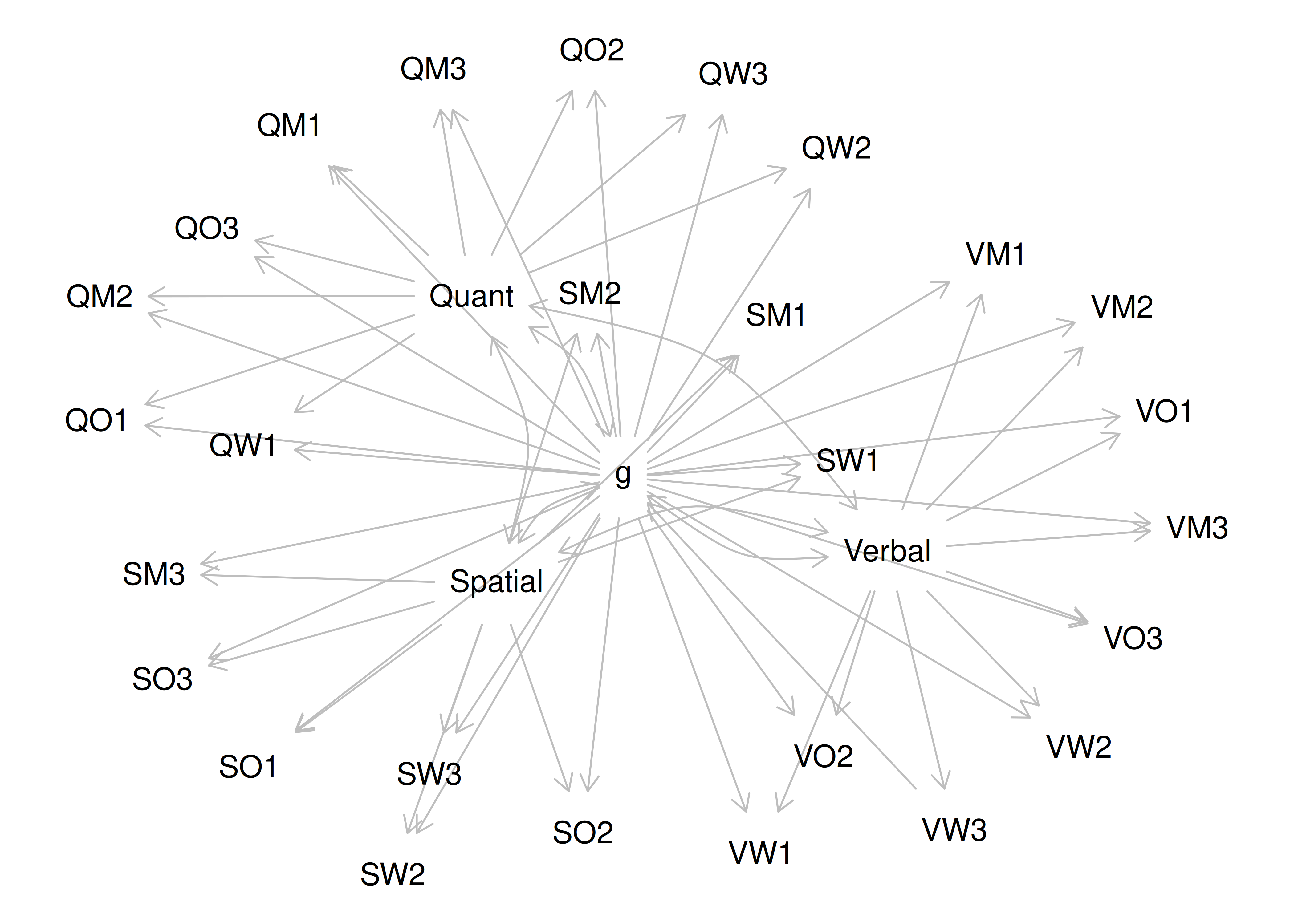
Figure 14.76: Equivalently Fitting Models to a Bifactor Model.
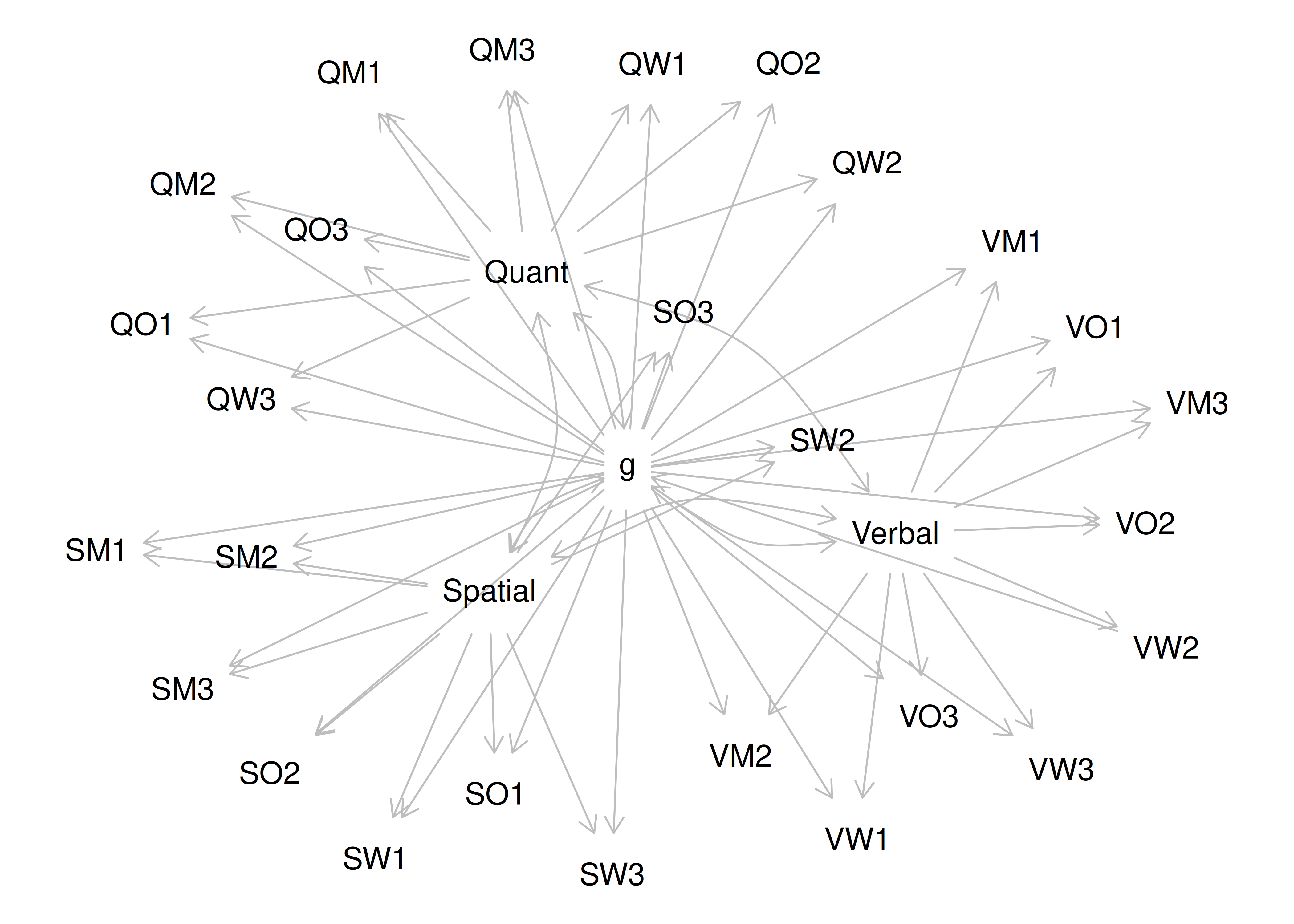
Figure 14.77: Equivalently Fitting Models to a Bifactor Model.
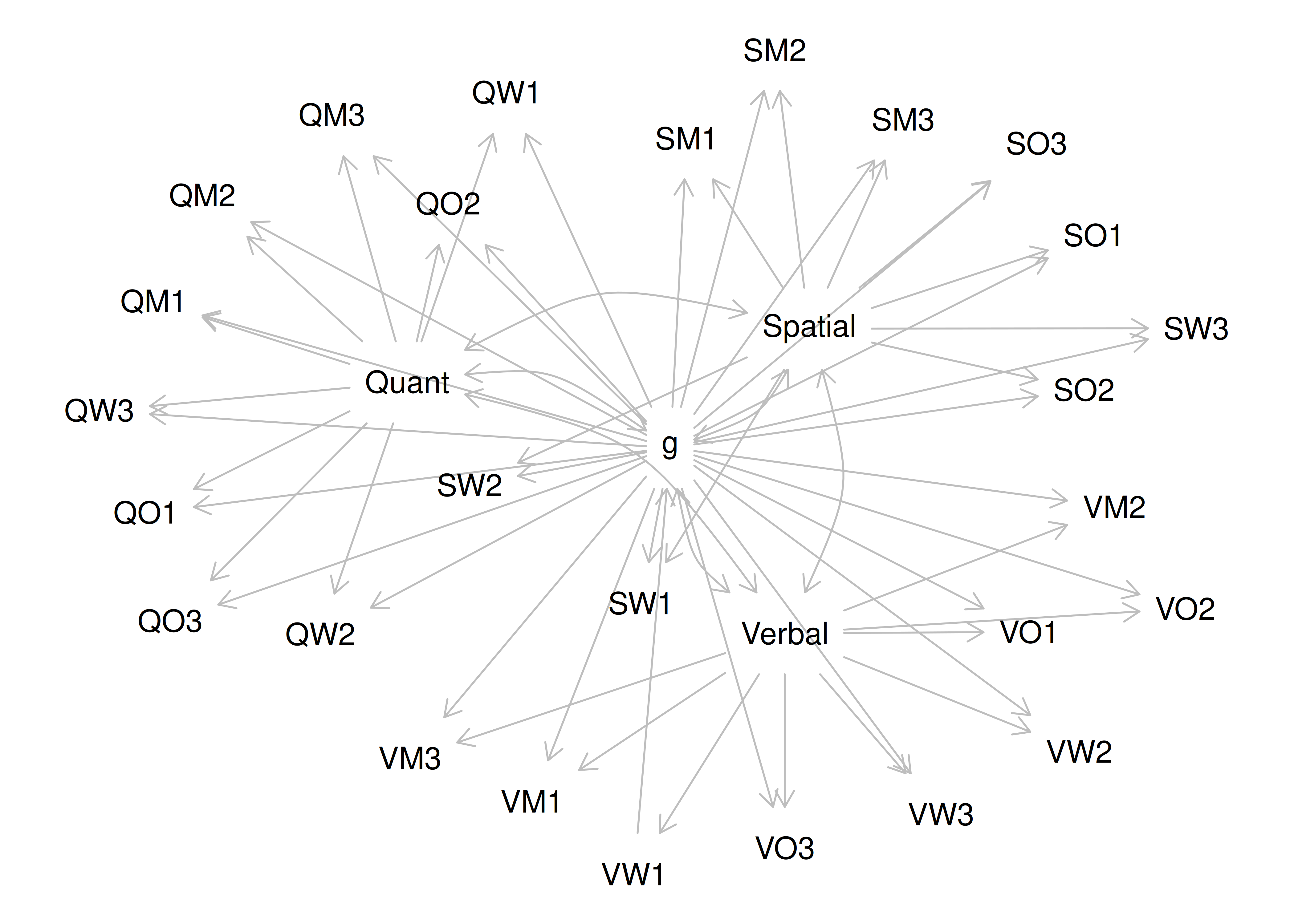
Figure 14.78: Equivalently Fitting Models to a Bifactor Model.
[[1]]
[[1]]$mar
[1] 0 0 0 0
[[2]]
[[2]]$mar
[1] 0 0 0 0
[[3]]
[[3]]$mar
[1] 0 0 0 0
[[4]]
[[4]]$mar
[1] 0 0 0 014.4.2.13 Multitrait-Multimethod Model (MTMM)
14.4.2.13.1 Simulate the data
We simulated the data for the multitrait-multimethod model (MTMM) in Section 5.3.1.4.2.3.
14.4.2.13.2 Specify the model
This example is courtesy of W. Joel Schneider.
Code
cfaModelMTMM_syntax <- '
g =~ Verbal + Spatial + Quant
Verbal =~
VO1 + VO2 + VO3 +
VW1 + VW2 + VW3 +
VM1 + VM2 + VM3
Spatial =~
SO1 + SO2 + SO3 +
SW1 + SW2 + SW3 +
SM1 + SM2 + SM3
Quant =~
QO1 + QO2 + QO3 +
QW1 + QW2 + QW3 +
QM1 + QM2 + QM3
Oral =~
VO1 + VO2 + VO3 +
SO1 + SO2 + SO3 +
QO1 + QO2 + QO3
Written =~
VW1 + VW2 + VW3 +
SW1 + SW2 + SW3 +
QW1 + QW2 + QW3
Manipulative =~
VM1 + VM2 + VM3 +
SM1 + SM2 + SM3 +
QM1 + QM2 + QM3
'
cfaModelMTMM_fullSyntax <- '
#Factor loadings (free the factor loading of the first indicator)
g =~ NA*Verbal + Spatial + Quant
Verbal =~
NA*VO1 + VO2 + VO3 +
VW1 + VW2 + VW3 +
VM1 + VM2 + VM3
Spatial =~
NA*SO1 + SO2 + SO3 +
SW1 + SW2 + SW3 +
SM1 + SM2 + SM3
Quant =~
NA*QO1 + QO2 + QO3 +
QW1 + QW2 + QW3 +
QM1 + QM2 + QM3
Oral =~
NA*VO1 + VO2 + VO3 +
SO1 + SO2 + SO3 +
QO1 + QO2 + QO3
Written =~
NA*VW1 + VW2 + VW3 +
SW1 + SW2 + SW3 +
QW1 + QW2 + QW3
Manipulative =~
NA*VM1 + VM2 + VM3 +
SM1 + SM2 + SM3 +
QM1 + QM2 + QM3
#Fix latent means to zero
Verbal ~ 0
Spatial ~ 0
Quant ~ 0
Oral ~ 0
Written ~ 0
Manipulative ~ 0
g ~ 0
#Fix latent variances to one
Verbal ~~ 1*Verbal
Spatial ~~ 1*Spatial
Quant ~~ 1*Quant
Oral ~~ 1*Oral
Written ~~ 1*Written
Manipulative ~~ 1*Manipulative
g ~~ 1*g
#Fix covariances among latent variables at zero
Verbal ~~ 0*Spatial
Verbal ~~ 0*Quant
Verbal ~~ 0*Oral
Verbal ~~ 0*Written
Verbal ~~ 0*Manipulative
Spatial ~~ 0*Quant
Spatial ~~ 0*Oral
Spatial ~~ 0*Written
Spatial ~~ 0*Manipulative
Quant ~~ 0*Oral
Quant ~~ 0*Written
Quant ~~ 0*Manipulative
Oral ~~ 0*Written
Oral ~~ 0*Manipulative
Written ~~ 0*Manipulative
g ~~ 0*Verbal
g ~~ 0*Spatial
g ~~ 0*Quant
g ~~ 0*Oral
g ~~ 0*Written
g ~~ 0*Manipulative
#Estimate residual variances of manifest variables
VO1 ~~ VO1
VO2 ~~ VO2
VO3 ~~ VO3
VW1 ~~ VW1
VW2 ~~ VW2
VW3 ~~ VW3
VM1 ~~ VM1
VM2 ~~ VM2
VM3 ~~ VM3
SO1 ~~ SO1
SO2 ~~ SO2
SO3 ~~ SO3
SW1 ~~ SW1
SW2 ~~ SW2
SW3 ~~ SW3
SM1 ~~ SM1
SM2 ~~ SM2
SM3 ~~ SM3
QO1 ~~ QO1
QO2 ~~ QO2
QO3 ~~ QO3
QW1 ~~ QW1
QW2 ~~ QW2
QW3 ~~ QW3
QM1 ~~ QM1
QM2 ~~ QM2
QM3 ~~ QM3
#Free intercepts of manifest variables
VO1 ~ intVO1*1
VO2 ~ intVO2*1
VO3 ~ intVO3*1
VW1 ~ intVW1*1
VW2 ~ intVW2*1
VW3 ~ intVW3*1
VM1 ~ intVM1*1
VM2 ~ intVM2*1
VM3 ~ intVM3*1
SO1 ~ intSO1*1
SO2 ~ intSO2*1
SO3 ~ intSO3*1
SW1 ~ intSW1*1
SW2 ~ intSW2*1
SW3 ~ intSW3*1
SM1 ~ intSM1*1
SM2 ~ intSM2*1
SM3 ~ intSM3*1
QO1 ~ intQO1*1
QO2 ~ intQO2*1
QO3 ~ intQO3*1
QW1 ~ intQW1*1
QW2 ~ intQW2*1
QW3 ~ intQW3*1
QM1 ~ intQM1*1
QM2 ~ intQM2*1
QM3 ~ intQM3*1
'14.4.2.13.5 Display summary output
lavaan 0.6-20 ended normally after 57 iterations
Estimator ML
Optimization method NLMINB
Number of model parameters 111
Number of observations 10000
Number of missing patterns 1
Model Test User Model:
Standard Scaled
Test Statistic 254.449 254.155
Degrees of freedom 294 294
P-value (Chi-square) 0.954 0.955
Scaling correction factor 1.001
Yuan-Bentler correction (Mplus variant)
Model Test Baseline Model:
Test statistic 146391.496 146201.022
Degrees of freedom 351 351
P-value 0.000 0.000
Scaling correction factor 1.001
User Model versus Baseline Model:
Comparative Fit Index (CFI) 1.000 1.000
Tucker-Lewis Index (TLI) 1.000 1.000
Robust Comparative Fit Index (CFI) 1.000
Robust Tucker-Lewis Index (TLI) 1.000
Loglikelihood and Information Criteria:
Loglikelihood user model (H0) -310030.970 -310030.970
Scaling correction factor 1.001
for the MLR correction
Loglikelihood unrestricted model (H1) -309903.745 -309903.745
Scaling correction factor 1.001
for the MLR correction
Akaike (AIC) 620283.939 620283.939
Bayesian (BIC) 621084.287 621084.287
Sample-size adjusted Bayesian (SABIC) 620731.545 620731.545
Root Mean Square Error of Approximation:
RMSEA 0.000 0.000
90 Percent confidence interval - lower 0.000 0.000
90 Percent confidence interval - upper 0.000 0.000
P-value H_0: RMSEA <= 0.050 1.000 1.000
P-value H_0: RMSEA >= 0.080 0.000 0.000
Robust RMSEA 0.000
90 Percent confidence interval - lower 0.000
90 Percent confidence interval - upper 0.000
P-value H_0: Robust RMSEA <= 0.050 1.000
P-value H_0: Robust RMSEA >= 0.080 0.000
Standardized Root Mean Square Residual:
SRMR 0.006 0.006
Parameter Estimates:
Standard errors Sandwich
Information bread Observed
Observed information based on Hessian
Latent Variables:
Estimate Std.Err z-value P(>|z|) Std.lv Std.all
g =~
Verbal 2.331 0.120 19.490 0.000 0.919 0.919
Spatial 1.194 0.029 41.325 0.000 0.767 0.767
Quant 0.858 0.019 44.320 0.000 0.651 0.651
Verbal =~
VO1 0.197 0.009 21.502 0.000 0.499 0.498
VO2 0.239 0.011 22.383 0.000 0.607 0.605
VO3 0.280 0.012 22.655 0.000 0.710 0.710
VW1 0.282 0.012 23.078 0.000 0.715 0.709
VW2 0.242 0.011 22.365 0.000 0.613 0.607
VW3 0.211 0.010 21.774 0.000 0.535 0.529
VM1 0.242 0.011 22.563 0.000 0.614 0.610
VM2 0.277 0.012 22.926 0.000 0.702 0.703
VM3 0.195 0.009 21.218 0.000 0.494 0.496
Spatial =~
SO1 0.445 0.008 57.171 0.000 0.693 0.699
SO2 0.450 0.008 56.641 0.000 0.700 0.700
SO3 0.383 0.007 52.516 0.000 0.597 0.596
SW1 0.384 0.007 57.093 0.000 0.598 0.597
SW2 0.450 0.007 62.843 0.000 0.700 0.701
SW3 0.323 0.007 47.171 0.000 0.502 0.505
SM1 0.455 0.007 60.751 0.000 0.709 0.713
SM2 0.317 0.007 44.502 0.000 0.493 0.495
SM3 0.456 0.007 64.320 0.000 0.709 0.712
Quant =~
QO1 0.380 0.007 51.830 0.000 0.501 0.504
QO2 0.523 0.008 67.618 0.000 0.689 0.694
QO3 0.386 0.008 48.712 0.000 0.508 0.504
QW1 0.386 0.008 50.153 0.000 0.509 0.506
QW2 0.447 0.007 61.478 0.000 0.588 0.595
QW3 0.527 0.007 75.098 0.000 0.695 0.696
QM1 0.381 0.008 49.115 0.000 0.502 0.504
QM2 0.450 0.008 57.056 0.000 0.593 0.590
QM3 0.535 0.008 68.983 0.000 0.705 0.702
Oral =~
VO1 0.405 0.011 36.849 0.000 0.405 0.404
VO2 0.494 0.010 49.808 0.000 0.494 0.492
VO3 0.297 0.010 29.548 0.000 0.297 0.297
SO1 0.293 0.010 29.258 0.000 0.293 0.295
SO2 0.297 0.010 29.825 0.000 0.297 0.296
SO3 0.512 0.010 50.395 0.000 0.512 0.512
QO1 0.583 0.011 55.071 0.000 0.583 0.587
QO2 0.310 0.010 31.012 0.000 0.310 0.312
QO3 0.402 0.011 36.601 0.000 0.402 0.399
Written =~
VW1 0.596 0.008 74.289 0.000 0.596 0.591
VW2 0.402 0.010 41.570 0.000 0.402 0.397
VW3 0.289 0.011 26.689 0.000 0.289 0.286
SW1 0.599 0.009 70.011 0.000 0.599 0.598
SW2 0.503 0.008 59.564 0.000 0.503 0.503
SW3 0.489 0.010 49.691 0.000 0.489 0.491
QW1 0.400 0.010 39.373 0.000 0.400 0.397
QW2 0.394 0.009 41.734 0.000 0.394 0.398
QW3 0.503 0.008 59.491 0.000 0.503 0.504
Manipulative =~
VM1 0.495 0.009 52.937 0.000 0.495 0.493
VM2 0.495 0.009 57.185 0.000 0.495 0.495
VM3 0.291 0.011 26.756 0.000 0.291 0.293
SM1 0.475 0.009 55.234 0.000 0.475 0.478
SM2 0.498 0.010 48.305 0.000 0.498 0.499
SM3 0.583 0.008 73.226 0.000 0.583 0.585
QM1 0.402 0.010 38.302 0.000 0.402 0.403
QM2 0.311 0.010 30.685 0.000 0.311 0.309
QM3 0.300 0.010 31.426 0.000 0.300 0.299
Covariances:
Estimate Std.Err z-value P(>|z|) Std.lv Std.all
g ~~
Oral 0.000 0.000 0.000
Written 0.000 0.000 0.000
Manipulative 0.000 0.000 0.000
Oral ~~
Written 0.000 0.000 0.000
Manipulative 0.000 0.000 0.000
Written ~~
Manipulative 0.000 0.000 0.000
Intercepts:
Estimate Std.Err z-value P(>|z|) Std.lv Std.all
.VO1 -0.007 0.010 -0.717 0.473 -0.007 -0.007
.VO2 -0.013 0.010 -1.254 0.210 -0.013 -0.013
.VO3 -0.008 0.010 -0.815 0.415 -0.008 -0.008
.VW1 0.015 0.010 1.464 0.143 0.015 0.015
.VW2 0.011 0.010 1.043 0.297 0.011 0.010
.VW3 -0.006 0.010 -0.572 0.567 -0.006 -0.006
.VM1 -0.011 0.010 -1.086 0.277 -0.011 -0.011
.VM2 -0.010 0.010 -0.992 0.321 -0.010 -0.010
.VM3 -0.012 0.010 -1.195 0.232 -0.012 -0.012
.SO1 -0.006 0.010 -0.588 0.557 -0.006 -0.006
.SO2 -0.014 0.010 -1.405 0.160 -0.014 -0.014
.SO3 -0.008 0.010 -0.827 0.408 -0.008 -0.008
.SW1 0.004 0.010 0.405 0.686 0.004 0.004
.SW2 0.007 0.010 0.673 0.501 0.007 0.007
.SW3 0.005 0.010 0.472 0.637 0.005 0.005
.SM1 -0.009 0.010 -0.913 0.361 -0.009 -0.009
.SM2 -0.008 0.010 -0.754 0.451 -0.008 -0.008
.SM3 -0.012 0.010 -1.185 0.236 -0.012 -0.012
.QO1 0.005 0.010 0.479 0.632 0.005 0.005
.QO2 0.005 0.010 0.458 0.647 0.005 0.005
.QO3 -0.001 0.010 -0.144 0.886 -0.001 -0.001
.QW1 0.010 0.010 0.950 0.342 0.010 0.009
.QW2 0.013 0.010 1.268 0.205 0.013 0.013
.QW3 0.025 0.010 2.555 0.011 0.025 0.026
.QM1 -0.000 0.010 -0.046 0.963 -0.000 -0.000
.QM2 0.009 0.010 0.876 0.381 0.009 0.009
.QM3 0.004 0.010 0.379 0.704 0.004 0.004
Variances:
Estimate Std.Err z-value P(>|z|) Std.lv Std.all
.VO1 0.591 0.009 63.350 0.000 0.591 0.589
.VO2 0.395 0.007 54.211 0.000 0.395 0.392
.VO3 0.407 0.007 56.302 0.000 0.407 0.408
.VW1 0.151 0.004 37.411 0.000 0.151 0.148
.VW2 0.485 0.007 64.821 0.000 0.485 0.474
.VW3 0.652 0.010 67.786 0.000 0.652 0.638
.VM1 0.389 0.007 57.784 0.000 0.389 0.385
.VM2 0.260 0.005 50.854 0.000 0.260 0.261
.VM3 0.662 0.010 66.688 0.000 0.662 0.668
.SO1 0.417 0.007 60.156 0.000 0.417 0.424
.SO2 0.423 0.007 59.184 0.000 0.423 0.423
.SO3 0.383 0.007 52.912 0.000 0.383 0.383
.SW1 0.287 0.005 52.962 0.000 0.287 0.286
.SW2 0.255 0.005 53.873 0.000 0.255 0.255
.SW3 0.499 0.008 65.345 0.000 0.499 0.504
.SM1 0.261 0.005 54.597 0.000 0.261 0.264
.SM2 0.503 0.008 63.845 0.000 0.503 0.506
.SM3 0.150 0.004 37.850 0.000 0.150 0.151
.QO1 0.396 0.008 47.010 0.000 0.396 0.402
.QO2 0.415 0.007 56.527 0.000 0.415 0.421
.QO3 0.595 0.009 63.503 0.000 0.595 0.586
.QW1 0.592 0.009 64.504 0.000 0.592 0.586
.QW2 0.475 0.008 61.934 0.000 0.475 0.487
.QW3 0.260 0.005 47.718 0.000 0.260 0.261
.QM1 0.581 0.009 64.008 0.000 0.581 0.584
.QM2 0.561 0.009 63.216 0.000 0.561 0.556
.QM3 0.420 0.008 55.556 0.000 0.420 0.417
g 1.000 1.000 1.000
.Verbal 1.000 0.155 0.155
.Spatial 1.000 0.412 0.412
.Quant 1.000 0.576 0.576
Oral 1.000 1.000 1.000
Written 1.000 1.000 1.000
Manipulative 1.000 1.000 1.000
R-Square:
Estimate
VO1 0.411
VO2 0.608
VO3 0.592
VW1 0.852
VW2 0.526
VW3 0.362
VM1 0.615
VM2 0.739
VM3 0.332
SO1 0.576
SO2 0.577
SO3 0.617
SW1 0.714
SW2 0.745
SW3 0.496
SM1 0.736
SM2 0.494
SM3 0.849
QO1 0.598
QO2 0.579
QO3 0.414
QW1 0.414
QW2 0.513
QW3 0.739
QM1 0.416
QM2 0.444
QM3 0.583
Verbal 0.845
Spatial 0.588
Quant 0.424lavaan 0.6-20 ended normally after 57 iterations
Estimator ML
Optimization method NLMINB
Number of model parameters 111
Number of observations 10000
Number of missing patterns 1
Model Test User Model:
Standard Scaled
Test Statistic 254.449 254.155
Degrees of freedom 294 294
P-value (Chi-square) 0.954 0.955
Scaling correction factor 1.001
Yuan-Bentler correction (Mplus variant)
Model Test Baseline Model:
Test statistic 146391.496 146201.022
Degrees of freedom 351 351
P-value 0.000 0.000
Scaling correction factor 1.001
User Model versus Baseline Model:
Comparative Fit Index (CFI) 1.000 1.000
Tucker-Lewis Index (TLI) 1.000 1.000
Robust Comparative Fit Index (CFI) 1.000
Robust Tucker-Lewis Index (TLI) 1.000
Loglikelihood and Information Criteria:
Loglikelihood user model (H0) -310030.970 -310030.970
Scaling correction factor 1.001
for the MLR correction
Loglikelihood unrestricted model (H1) -309903.745 -309903.745
Scaling correction factor 1.001
for the MLR correction
Akaike (AIC) 620283.939 620283.939
Bayesian (BIC) 621084.287 621084.287
Sample-size adjusted Bayesian (SABIC) 620731.545 620731.545
Root Mean Square Error of Approximation:
RMSEA 0.000 0.000
90 Percent confidence interval - lower 0.000 0.000
90 Percent confidence interval - upper 0.000 0.000
P-value H_0: RMSEA <= 0.050 1.000 1.000
P-value H_0: RMSEA >= 0.080 0.000 0.000
Robust RMSEA 0.000
90 Percent confidence interval - lower 0.000
90 Percent confidence interval - upper 0.000
P-value H_0: Robust RMSEA <= 0.050 1.000
P-value H_0: Robust RMSEA >= 0.080 0.000
Standardized Root Mean Square Residual:
SRMR 0.006 0.006
Parameter Estimates:
Standard errors Sandwich
Information bread Observed
Observed information based on Hessian
Latent Variables:
Estimate Std.Err z-value P(>|z|) Std.lv Std.all
g =~
Verbal 2.331 0.120 19.490 0.000 0.919 0.919
Spatial 1.194 0.029 41.325 0.000 0.767 0.767
Quant 0.858 0.019 44.320 0.000 0.651 0.651
Verbal =~
VO1 0.197 0.009 21.502 0.000 0.499 0.498
VO2 0.239 0.011 22.383 0.000 0.607 0.605
VO3 0.280 0.012 22.655 0.000 0.710 0.710
VW1 0.282 0.012 23.078 0.000 0.715 0.709
VW2 0.242 0.011 22.365 0.000 0.613 0.607
VW3 0.211 0.010 21.774 0.000 0.535 0.529
VM1 0.242 0.011 22.563 0.000 0.614 0.610
VM2 0.277 0.012 22.926 0.000 0.702 0.703
VM3 0.195 0.009 21.218 0.000 0.494 0.496
Spatial =~
SO1 0.445 0.008 57.171 0.000 0.693 0.699
SO2 0.450 0.008 56.641 0.000 0.700 0.700
SO3 0.383 0.007 52.516 0.000 0.597 0.596
SW1 0.384 0.007 57.093 0.000 0.598 0.597
SW2 0.450 0.007 62.843 0.000 0.700 0.701
SW3 0.323 0.007 47.171 0.000 0.502 0.505
SM1 0.455 0.007 60.751 0.000 0.709 0.713
SM2 0.317 0.007 44.502 0.000 0.493 0.495
SM3 0.456 0.007 64.320 0.000 0.709 0.712
Quant =~
QO1 0.380 0.007 51.830 0.000 0.501 0.504
QO2 0.523 0.008 67.618 0.000 0.689 0.694
QO3 0.386 0.008 48.712 0.000 0.508 0.504
QW1 0.386 0.008 50.153 0.000 0.509 0.506
QW2 0.447 0.007 61.478 0.000 0.588 0.595
QW3 0.527 0.007 75.098 0.000 0.695 0.696
QM1 0.381 0.008 49.115 0.000 0.502 0.504
QM2 0.450 0.008 57.056 0.000 0.593 0.590
QM3 0.535 0.008 68.983 0.000 0.705 0.702
Oral =~
VO1 0.405 0.011 36.849 0.000 0.405 0.404
VO2 0.494 0.010 49.808 0.000 0.494 0.492
VO3 0.297 0.010 29.548 0.000 0.297 0.297
SO1 0.293 0.010 29.258 0.000 0.293 0.295
SO2 0.297 0.010 29.825 0.000 0.297 0.296
SO3 0.512 0.010 50.395 0.000 0.512 0.512
QO1 0.583 0.011 55.071 0.000 0.583 0.587
QO2 0.310 0.010 31.012 0.000 0.310 0.312
QO3 0.402 0.011 36.601 0.000 0.402 0.399
Written =~
VW1 0.596 0.008 74.289 0.000 0.596 0.591
VW2 0.402 0.010 41.570 0.000 0.402 0.397
VW3 0.289 0.011 26.689 0.000 0.289 0.286
SW1 0.599 0.009 70.011 0.000 0.599 0.598
SW2 0.503 0.008 59.564 0.000 0.503 0.503
SW3 0.489 0.010 49.691 0.000 0.489 0.491
QW1 0.400 0.010 39.373 0.000 0.400 0.397
QW2 0.394 0.009 41.734 0.000 0.394 0.398
QW3 0.503 0.008 59.491 0.000 0.503 0.504
Manipulative =~
VM1 0.495 0.009 52.937 0.000 0.495 0.493
VM2 0.495 0.009 57.185 0.000 0.495 0.495
VM3 0.291 0.011 26.756 0.000 0.291 0.293
SM1 0.475 0.009 55.234 0.000 0.475 0.478
SM2 0.498 0.010 48.305 0.000 0.498 0.499
SM3 0.583 0.008 73.226 0.000 0.583 0.585
QM1 0.402 0.010 38.302 0.000 0.402 0.403
QM2 0.311 0.010 30.685 0.000 0.311 0.309
QM3 0.300 0.010 31.426 0.000 0.300 0.299
Covariances:
Estimate Std.Err z-value P(>|z|) Std.lv Std.all
.Verbal ~~
.Spatial 0.000 0.000 0.000
.Quant 0.000 0.000 0.000
Oral 0.000 0.000 0.000
Written 0.000 0.000 0.000
Manipulative 0.000 0.000 0.000
.Spatial ~~
.Quant 0.000 0.000 0.000
Oral 0.000 0.000 0.000
Written 0.000 0.000 0.000
Manipulative 0.000 0.000 0.000
.Quant ~~
Oral 0.000 0.000 0.000
Written 0.000 0.000 0.000
Manipulative 0.000 0.000 0.000
Oral ~~
Written 0.000 0.000 0.000
Manipulative 0.000 0.000 0.000
Written ~~
Manipulative 0.000 0.000 0.000
g ~~
.Verbal 0.000 0.000 0.000
.Spatial 0.000 0.000 0.000
.Quant 0.000 0.000 0.000
Oral 0.000 0.000 0.000
Written 0.000 0.000 0.000
Manipulative 0.000 0.000 0.000
Intercepts:
Estimate Std.Err z-value P(>|z|) Std.lv Std.all
.Verbal 0.000 0.000 0.000
.Spatial 0.000 0.000 0.000
.Quant 0.000 0.000 0.000
Oral 0.000 0.000 0.000
Written 0.000 0.000 0.000
Manpltv 0.000 0.000 0.000
g 0.000 0.000 0.000
.VO1 (iVO1) -0.007 0.010 -0.717 0.473 -0.007 -0.007
.VO2 (iVO2) -0.013 0.010 -1.254 0.210 -0.013 -0.013
.VO3 (iVO3) -0.008 0.010 -0.815 0.415 -0.008 -0.008
.VW1 (iVW1) 0.015 0.010 1.464 0.143 0.015 0.015
.VW2 (iVW2) 0.011 0.010 1.043 0.297 0.011 0.010
.VW3 (iVW3) -0.006 0.010 -0.572 0.567 -0.006 -0.006
.VM1 (iVM1) -0.011 0.010 -1.086 0.277 -0.011 -0.011
.VM2 (iVM2) -0.010 0.010 -0.992 0.321 -0.010 -0.010
.VM3 (iVM3) -0.012 0.010 -1.195 0.232 -0.012 -0.012
.SO1 (iSO1) -0.006 0.010 -0.588 0.557 -0.006 -0.006
.SO2 (iSO2) -0.014 0.010 -1.405 0.160 -0.014 -0.014
.SO3 (iSO3) -0.008 0.010 -0.827 0.408 -0.008 -0.008
.SW1 (iSW1) 0.004 0.010 0.405 0.686 0.004 0.004
.SW2 (iSW2) 0.007 0.010 0.673 0.501 0.007 0.007
.SW3 (iSW3) 0.005 0.010 0.472 0.637 0.005 0.005
.SM1 (iSM1) -0.009 0.010 -0.913 0.361 -0.009 -0.009
.SM2 (iSM2) -0.008 0.010 -0.754 0.451 -0.008 -0.008
.SM3 (iSM3) -0.012 0.010 -1.185 0.236 -0.012 -0.012
.QO1 (iQO1) 0.005 0.010 0.479 0.632 0.005 0.005
.QO2 (iQO2) 0.005 0.010 0.458 0.647 0.005 0.005
.QO3 (iQO3) -0.001 0.010 -0.144 0.886 -0.001 -0.001
.QW1 (iQW1) 0.010 0.010 0.950 0.342 0.010 0.009
.QW2 (iQW2) 0.013 0.010 1.268 0.205 0.013 0.013
.QW3 (iQW3) 0.025 0.010 2.555 0.011 0.025 0.026
.QM1 (iQM1) -0.000 0.010 -0.046 0.963 -0.000 -0.000
.QM2 (iQM2) 0.009 0.010 0.876 0.381 0.009 0.009
.QM3 (iQM3) 0.004 0.010 0.379 0.704 0.004 0.004
Variances:
Estimate Std.Err z-value P(>|z|) Std.lv Std.all
.Verbal 1.000 0.155 0.155
.Spatial 1.000 0.412 0.412
.Quant 1.000 0.576 0.576
Oral 1.000 1.000 1.000
Written 1.000 1.000 1.000
Manipulative 1.000 1.000 1.000
g 1.000 1.000 1.000
.VO1 0.591 0.009 63.350 0.000 0.591 0.589
.VO2 0.395 0.007 54.211 0.000 0.395 0.392
.VO3 0.407 0.007 56.302 0.000 0.407 0.408
.VW1 0.151 0.004 37.411 0.000 0.151 0.148
.VW2 0.485 0.007 64.821 0.000 0.485 0.474
.VW3 0.652 0.010 67.786 0.000 0.652 0.638
.VM1 0.389 0.007 57.784 0.000 0.389 0.385
.VM2 0.260 0.005 50.854 0.000 0.260 0.261
.VM3 0.662 0.010 66.688 0.000 0.662 0.668
.SO1 0.417 0.007 60.156 0.000 0.417 0.424
.SO2 0.423 0.007 59.184 0.000 0.423 0.423
.SO3 0.383 0.007 52.912 0.000 0.383 0.383
.SW1 0.287 0.005 52.962 0.000 0.287 0.286
.SW2 0.255 0.005 53.873 0.000 0.255 0.255
.SW3 0.499 0.008 65.345 0.000 0.499 0.504
.SM1 0.261 0.005 54.597 0.000 0.261 0.264
.SM2 0.503 0.008 63.845 0.000 0.503 0.506
.SM3 0.150 0.004 37.850 0.000 0.150 0.151
.QO1 0.396 0.008 47.010 0.000 0.396 0.402
.QO2 0.415 0.007 56.527 0.000 0.415 0.421
.QO3 0.595 0.009 63.503 0.000 0.595 0.586
.QW1 0.592 0.009 64.504 0.000 0.592 0.586
.QW2 0.475 0.008 61.934 0.000 0.475 0.487
.QW3 0.260 0.005 47.718 0.000 0.260 0.261
.QM1 0.581 0.009 64.008 0.000 0.581 0.584
.QM2 0.561 0.009 63.216 0.000 0.561 0.556
.QM3 0.420 0.008 55.556 0.000 0.420 0.417
R-Square:
Estimate
Verbal 0.845
Spatial 0.588
Quant 0.424
VO1 0.411
VO2 0.608
VO3 0.592
VW1 0.852
VW2 0.526
VW3 0.362
VM1 0.615
VM2 0.739
VM3 0.332
SO1 0.576
SO2 0.577
SO3 0.617
SW1 0.714
SW2 0.745
SW3 0.496
SM1 0.736
SM2 0.494
SM3 0.849
QO1 0.598
QO2 0.579
QO3 0.414
QW1 0.414
QW2 0.513
QW3 0.739
QM1 0.416
QM2 0.444
QM3 0.58314.4.2.13.6 Estimates of model fit
Code
chisq df pvalue
254.449 294.000 0.954
chisq.scaled df.scaled pvalue.scaled
254.155 294.000 0.955
chisq.scaling.factor baseline.chisq baseline.df
1.001 146391.496 351.000
baseline.pvalue rmsea cfi
0.000 0.000 1.000
tli srmr rmsea.robust
1.000 0.006 0.000
cfi.robust tli.robust
1.000 1.000 14.4.2.13.7 Residuals
$type
[1] "cor.bollen"
$cov
VO1 VO2 VO3 VW1 VW2 VW3 VM1 VM2 VM3 SO1
VO1 0.000
VO2 -0.003 0.000
VO3 0.001 -0.002 0.000
VW1 -0.005 0.005 -0.005 0.000
VW2 -0.004 -0.001 0.000 0.000 0.000
VW3 0.002 -0.007 -0.005 0.001 -0.002 0.000
VM1 0.001 0.001 0.007 0.001 -0.008 0.004 0.000
VM2 0.008 -0.002 0.006 0.000 0.002 -0.001 -0.001 0.000
VM3 0.003 0.005 0.002 0.001 0.004 -0.009 0.010 0.000 0.000
SO1 -0.005 -0.003 -0.002 0.007 0.002 0.001 0.003 -0.004 -0.003 0.000
SO2 -0.010 -0.006 -0.007 0.001 0.002 0.004 -0.004 -0.007 -0.005 -0.001
SO3 0.003 -0.002 -0.003 -0.004 0.003 -0.005 -0.005 -0.012 0.007 -0.003
SW1 -0.012 -0.003 -0.008 0.002 0.007 -0.009 0.000 -0.006 0.000 0.002
SW2 -0.003 -0.007 -0.006 0.001 0.003 0.010 0.011 0.002 0.002 0.000
SW3 -0.002 0.003 -0.005 0.000 0.001 0.002 0.007 -0.001 0.003 0.001
SM1 0.001 -0.002 0.001 0.001 0.010 -0.009 0.002 -0.001 0.000 -0.001
SM2 0.005 -0.004 0.013 0.001 0.003 -0.001 0.004 0.002 0.005 -0.002
SM3 0.009 0.004 0.005 0.006 0.006 0.004 0.005 0.002 0.002 -0.001
QO1 0.000 0.001 0.004 0.002 -0.001 0.002 -0.001 0.008 0.001 -0.004
QO2 -0.011 -0.012 -0.002 -0.011 0.000 0.007 -0.003 0.000 0.007 -0.004
QO3 -0.010 -0.005 -0.001 -0.010 -0.015 -0.008 -0.007 -0.004 -0.003 -0.004
QW1 0.003 0.003 0.008 0.004 -0.005 0.010 0.004 -0.001 0.009 0.007
QW2 -0.010 -0.010 -0.002 0.002 0.003 0.005 0.007 0.002 0.012 0.002
QW3 -0.015 -0.009 -0.006 -0.006 -0.007 0.001 -0.005 -0.004 -0.005 -0.003
QM1 -0.011 0.000 0.009 -0.007 -0.002 0.008 0.005 -0.004 -0.002 0.001
QM2 -0.006 -0.005 0.009 -0.003 0.000 0.009 0.001 -0.001 -0.013 -0.003
QM3 -0.001 0.001 0.012 0.014 0.003 0.015 0.007 0.011 0.006 -0.002
SO2 SO3 SW1 SW2 SW3 SM1 SM2 SM3 QO1 QO2
VO1
VO2
VO3
VW1
VW2
VW3
VM1
VM2
VM3
SO1
SO2 0.000
SO3 0.001 0.000
SW1 0.009 -0.013 0.000
SW2 -0.004 -0.007 0.000 0.000
SW3 0.006 -0.004 -0.001 0.004 0.000
SM1 -0.001 -0.003 0.003 0.005 0.000 0.000
SM2 -0.006 0.002 -0.003 0.000 0.007 0.000 0.000
SM3 -0.002 -0.001 0.001 0.006 0.002 0.000 0.002 0.000
QO1 -0.003 -0.010 -0.013 -0.008 -0.002 -0.007 -0.006 0.000 0.000
QO2 -0.006 0.000 -0.016 -0.002 -0.008 -0.005 -0.002 0.000 0.000 0.000
QO3 -0.009 -0.012 -0.016 -0.008 -0.009 -0.009 -0.009 -0.002 -0.002 -0.001
QW1 0.007 0.000 0.000 0.004 0.000 0.002 -0.010 0.002 0.009 -0.005
QW2 0.004 -0.010 -0.004 0.012 0.005 0.017 0.003 0.010 -0.012 -0.008
QW3 0.005 -0.009 -0.005 0.001 0.006 -0.001 -0.009 -0.002 -0.008 -0.007
QM1 -0.003 0.008 -0.006 0.005 0.010 0.010 -0.008 0.003 -0.005 -0.008
QM2 0.000 -0.005 0.004 -0.003 0.005 0.003 -0.004 0.003 0.004 0.006
QM3 -0.005 -0.002 0.000 0.011 0.009 -0.001 0.001 0.002 -0.008 0.001
QO3 QW1 QW2 QW3 QM1 QM2 QM3
VO1
VO2
VO3
VW1
VW2
VW3
VM1
VM2
VM3
SO1
SO2
SO3
SW1
SW2
SW3
SM1
SM2
SM3
QO1
QO2
QO3 0.000
QW1 0.003 0.000
QW2 -0.007 -0.003 0.000
QW3 -0.001 0.000 -0.001 0.000
QM1 -0.010 0.004 -0.001 0.002 0.000
QM2 -0.004 0.000 0.001 0.001 0.000 0.000
QM3 -0.005 -0.004 0.007 0.003 0.006 -0.006 0.000
$mean
VO1 VO2 VO3 VW1 VW2 VW3 VM1 VM2 VM3 SO1 SO2 SO3 SW1 SW2 SW3 SM1 SM2 SM3 QO1 QO2
0 0 0 0 0 0 0 0 0 0 0 0 0 0 0 0 0 0 0 0
QO3 QW1 QW2 QW3 QM1 QM2 QM3
0 0 0 0 0 0 0 14.4.2.13.9 Internal Consistency Reliability
Internal consistency reliability of items composing the latent factors, as quantified by omega (\(\omega\)) and average variance extracted (AVE), was estimated using the semTools package (Jorgensen et al., 2021).
Verbal Spatial Quant Oral Written Manipulative
0.775 0.777 0.767 0.332 0.404 0.360 Verbal Spatial Quant Oral Written Manipulative
0.775 0.777 0.767 0.332 0.404 0.360
g
0.646 Verbal Spatial Quant Oral Written Manipulative
NA NA NA NA NA NA 14.4.2.13.10 Bifactor Indices
$FactorLevelIndices
ECV_SS Omega OmegaH H FD
g NaN NaN NaN 0.0000000 0.0000000
Verbal 0.6711988 0.8971234 0.7754937 0.8529355 0.2653193
Spatial 0.6368848 0.9240480 0.7769438 0.8703888 0.5418020
Quant 0.6766914 0.8830017 0.7633144 0.8410966 0.6552951
Oral 0.3080222 0.8514506 0.4766152 0.6645373 0.8401561
Written 0.3752644 0.8821328 0.5620303 0.7328789 0.8965987
Manipulative 0.3341059 0.8684448 0.5150787 0.6954478 0.874549014.4.2.13.11 Path diagram
A path diagram of the model generated using the semPlot package (Epskamp, 2022) is in Figure 14.79.
Code
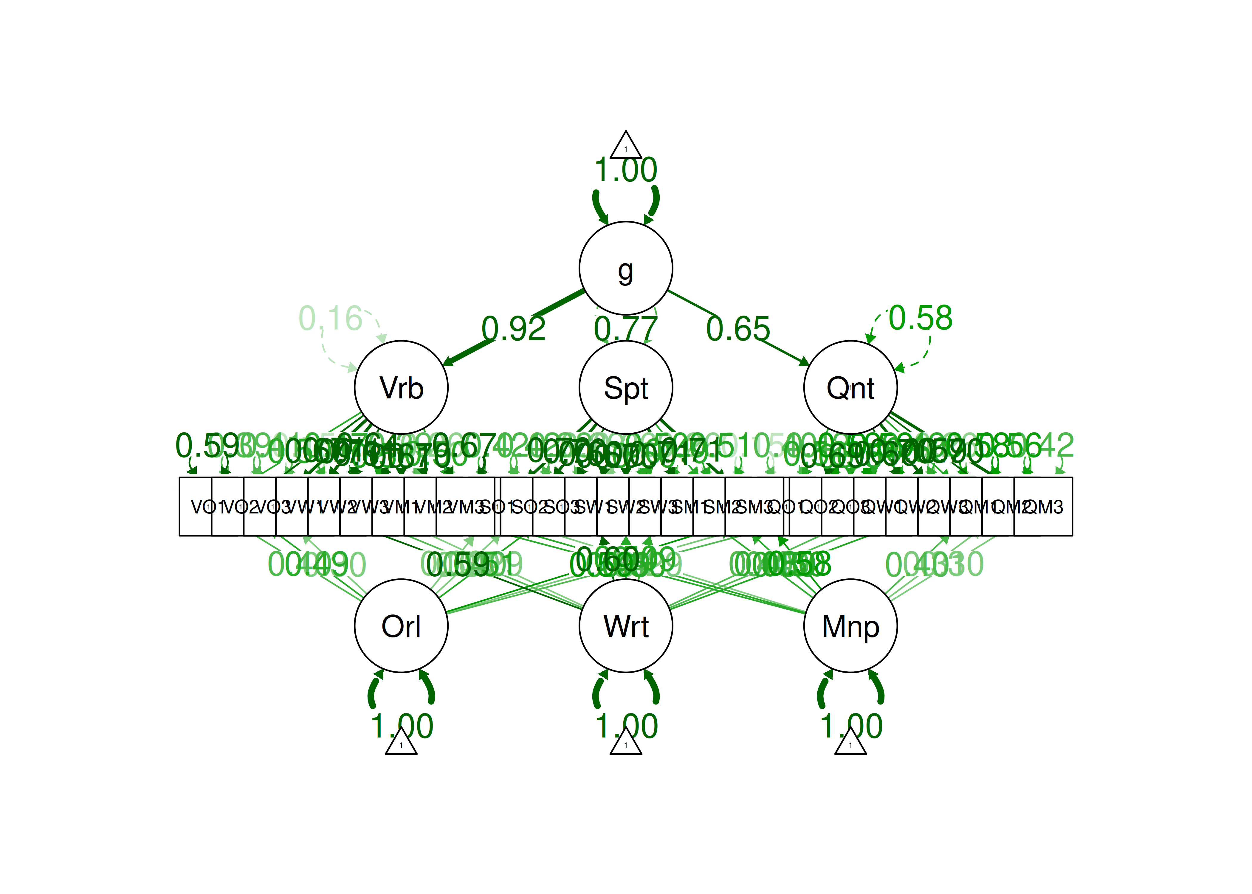
Figure 14.79: Multitrait-Multimethod Model in Confirmatory Factor Analysis.
14.4.2.13.12 Equivalently fitting models
Markov equivalent directed acyclic graphs (DAGs) were depicted using the dagitty package (Textor et al., 2021).
Path diagrams of equivalently fitting models are below.
Figure 14.80: Equivalently Fitting Models to a Multitrait-Multimethod Model in Confirmatory Factor Analysis.
Figure 14.81: Equivalently Fitting Models to a Multitrait-Multimethod Model in Confirmatory Factor Analysis.
Figure 14.82: Equivalently Fitting Models to a Multitrait-Multimethod Model in Confirmatory Factor Analysis.
Figure 14.83: Equivalently Fitting Models to a Multitrait-Multimethod Model in Confirmatory Factor Analysis.
[[1]]
[[1]]$mar
[1] 0 0 0 0
[[2]]
[[2]]$mar
[1] 0 0 0 0
[[3]]
[[3]]$mar
[1] 0 0 0 0
[[4]]
[[4]]$mar
[1] 0 0 0 014.4.3 Exploratory Structural Equation Model (ESEM)
14.4.3.1 Example 1
14.4.3.1.1 Specify the model
To specify an exploratory structural equation model (ESEM), you use the factor loadings from an EFA model as the starting values in a structural equation model. In this example, I use the factor loadings from the three-factor EFA model, as specified in Section 14.4.1.2.2.2. The factor loadings are in Table ??.
Code
In ESEM, you specify one anchor item for each latent factor. You want the anchor item to be an item that has a strong loading on one latent factor and to have weak loadings on every other latent factor. The cross-loadings for the anchor item are fixed to the respective loadings from the original EFA model. I specify an anchor item for each latent factor below:
The petersenlab package (Petersen, 2025) includes the make_esem_model() function that creates lavaan syntax for an ESEM model from the factor loadings of an EFA model, as adapted from Mateus Silvestrin: https://msilvestrin.me/post/esem (archived at https://perma.cc/FA8D-4NB9)
f1 =~ start(0.731519509523096)*x1+start(0.583748291703279)*x2+start(0.847715845553109)*x3+start(0.0061224618573914)*x4+-0.00498246092331398*x5+start(0.0966229010843947)*x6+-0.00106786089007843*x7+start(0.283600555518608)*x8+start(0.496276934979204)*x9
f2 =~ start(0.139474772562034)*x1+start(-0.00800945479356107)*x2+-0.145067349472644*x3+start(0.990877224285709)*x4+start(1.12736460983691)*x5+start(0.804382018891042)*x6+0.0602438955885163*x7+start(-0.00753284252626253)*x8+start(0.00782360464751289)*x9
f3 =~ start(-0.0429741160104005)*x1+start(-0.179604539350993)*x2+0.00636247165395365*x3+start(0.00736980647162112)*x4+0.0341008215410021*x5+start(-0.00133134414552763)*x6+start(0.755705714528228)*x7+start(0.638194636667683)*x8+start(0.432390891115082)*x9 14.4.3.1.4 Display summary output
lavaan 0.6-20 ended normally after 93 iterations
Estimator ML
Optimization method NLMINB
Number of model parameters 42
Number of observations 301
Number of missing patterns 75
Model Test User Model:
Standard Scaled
Test Statistic 23.051 23.723
Degrees of freedom 12 12
P-value (Chi-square) 0.027 0.022
Scaling correction factor 0.972
Yuan-Bentler correction (Mplus variant)
Model Test Baseline Model:
Test statistic 693.305 646.574
Degrees of freedom 36 36
P-value 0.000 0.000
Scaling correction factor 1.072
User Model versus Baseline Model:
Comparative Fit Index (CFI) 0.983 0.981
Tucker-Lewis Index (TLI) 0.950 0.942
Robust Comparative Fit Index (CFI) 0.980
Robust Tucker-Lewis Index (TLI) 0.939
Loglikelihood and Information Criteria:
Loglikelihood user model (H0) -3192.304 -3192.304
Scaling correction factor 1.090
for the MLR correction
Loglikelihood unrestricted model (H1) -3180.778 -3180.778
Scaling correction factor 1.064
for the MLR correction
Akaike (AIC) 6468.608 6468.608
Bayesian (BIC) 6624.307 6624.307
Sample-size adjusted Bayesian (SABIC) 6491.107 6491.107
Root Mean Square Error of Approximation:
RMSEA 0.055 0.057
90 Percent confidence interval - lower 0.018 0.020
90 Percent confidence interval - upper 0.089 0.091
P-value H_0: RMSEA <= 0.050 0.358 0.329
P-value H_0: RMSEA >= 0.080 0.124 0.144
Robust RMSEA 0.070
90 Percent confidence interval - lower 0.017
90 Percent confidence interval - upper 0.115
P-value H_0: Robust RMSEA <= 0.050 0.215
P-value H_0: Robust RMSEA >= 0.080 0.393
Standardized Root Mean Square Residual:
SRMR 0.020 0.020
Parameter Estimates:
Standard errors Sandwich
Information bread Observed
Observed information based on Hessian
Latent Variables:
Estimate Std.Err z-value P(>|z|) Std.lv Std.all
f1 =~
x1 0.732 0.732 0.632
x2 0.584 0.131 4.442 0.000 0.584 0.505
x3 0.848 0.182 4.661 0.000 0.848 0.753
x4 0.006 0.105 0.058 0.954 0.006 0.005
x5 -0.005 -0.005 -0.004
x6 0.097 0.087 1.108 0.268 0.097 0.093
x7 -0.001 -0.001 -0.001
x8 0.284 0.112 2.539 0.011 0.284 0.280
x9 0.496 0.123 4.023 0.000 0.496 0.487
f2 =~
x1 0.139 0.139 0.120
x2 -0.008 0.098 -0.082 0.935 -0.008 -0.007
x3 -0.145 -0.145 -0.129
x4 0.991 0.401 2.472 0.013 0.991 0.843
x5 1.127 0.442 2.549 0.011 1.127 0.869
x6 0.804 0.333 2.414 0.016 0.804 0.774
x7 0.060 0.060 0.056
x8 -0.008 0.090 -0.083 0.934 -0.008 -0.007
x9 0.008 0.075 0.104 0.917 0.008 0.008
f3 =~
x1 -0.043 -0.043 -0.037
x2 -0.180 0.325 -0.553 0.580 -0.180 -0.155
x3 0.006 0.006 0.006
x4 0.007 0.117 0.063 0.950 0.007 0.006
x5 0.034 0.034 0.026
x6 -0.001 0.090 -0.015 0.988 -0.001 -0.001
x7 0.756 1.429 0.529 0.597 0.756 0.708
x8 0.638 1.337 0.477 0.633 0.638 0.630
x9 0.432 0.884 0.489 0.625 0.432 0.424
Covariances:
Estimate Std.Err z-value P(>|z|) Std.lv Std.all
f1 ~~
f2 0.396 0.178 2.228 0.026 0.396 0.396
f3 0.112 0.260 0.432 0.666 0.112 0.112
f2 ~~
f3 0.107 0.164 0.654 0.513 0.107 0.107
Intercepts:
Estimate Std.Err z-value P(>|z|) Std.lv Std.all
.x1 4.974 0.071 69.866 0.000 4.974 4.297
.x2 6.047 0.070 86.533 0.000 6.047 5.230
.x3 2.221 0.069 32.224 0.000 2.221 1.971
.x4 3.095 0.071 43.794 0.000 3.095 2.634
.x5 4.341 0.078 55.604 0.000 4.341 3.347
.x6 2.188 0.064 34.270 0.000 2.188 2.104
.x7 4.177 0.064 64.895 0.000 4.177 3.914
.x8 5.520 0.062 89.727 0.000 5.520 5.449
.x9 5.401 0.063 86.038 0.000 5.401 5.297
Variances:
Estimate Std.Err z-value P(>|z|) Std.lv Std.all
.x1 0.711 0.121 5.855 0.000 0.711 0.531
.x2 0.991 0.119 8.325 0.000 0.991 0.741
.x3 0.626 0.124 5.040 0.000 0.626 0.493
.x4 0.393 0.073 5.413 0.000 0.393 0.284
.x5 0.406 0.084 4.836 0.000 0.406 0.241
.x6 0.364 0.054 6.681 0.000 0.364 0.336
.x7 0.555 0.174 3.188 0.001 0.555 0.487
.x8 0.501 0.117 4.291 0.000 0.501 0.488
.x9 0.554 0.073 7.638 0.000 0.554 0.533
f1 1.000 0.294 3.402 0.001 1.000 1.000
f2 1.000 0.796 1.256 0.209 1.000 1.000
f3 1.000 3.947 0.253 0.800 1.000 1.000
R-Square:
Estimate
x1 0.469
x2 0.259
x3 0.507
x4 0.716
x5 0.759
x6 0.664
x7 0.513
x8 0.512
x9 0.46714.4.3.1.5 Estimates of model fit
Code
chisq df pvalue
23.051 12.000 0.027
chisq.scaled df.scaled pvalue.scaled
23.723 12.000 0.022
chisq.scaling.factor baseline.chisq baseline.df
0.972 693.305 36.000
baseline.pvalue rmsea cfi
0.000 0.055 0.983
tli srmr rmsea.robust
0.950 0.020 0.070
cfi.robust tli.robust
0.980 0.939 14.4.3.1.6 Nested model comparison
A nested model comparison indicates that the ESEM model fits significantly better than the CFA model.
14.4.3.1.7 Residuals
$type
[1] "cor.bollen"

$cov
       x1     x2     x3     x4     x5     x6     x7     x8     x9
x1  0.000
x2 -0.008  0.000
x3  0.001 -0.004  0.000
x4  0.040 -0.022 -0.001  0.000
x5 -0.019  0.013 -0.031 -0.004  0.000
x6 -0.034  0.015  0.024 -0.002  0.005  0.000
x7 -0.034 -0.037  0.027  0.035 -0.043  0.001  0.000
x8  0.027  0.029 -0.041 -0.044  0.016  0.016 -0.007  0.000
x9 -0.010  0.013  0.014 -0.033  0.042 -0.024 -0.009 -0.002  0.000

$mean
    x1     x2     x3     x4     x5     x6     x7     x8     x9
0.003 -0.001 0.003 -0.003 -0.001 0.005 0.003 -0.001 0.003 14.4.3.1.9 Internal Consistency Reliability
Internal consistency reliability of items composing the latent factors, as quantified by omega (\(\omega\)) and average variance extracted (AVE), was estimated using the semTools package (Jorgensen et al., 2021).
f1 f2 f3
0.264 0.252 0.078 f1 f2 f3
NA NA NA 14.4.3.1.10 Path diagram
A path diagram of the model generated using the semPlot package (Epskamp, 2022) is in Figure 14.84.

Figure 14.84: Exploratory Structural Equation Model With All Cross-loadings.
14.4.3.1.11 Equivalently fitting models
Markov equivalent directed acyclic graphs (DAGs) were depicted using the dagitty package (Textor et al., 2021).
Path diagrams of equivalent models are below.
Figure 14.85: Equivalently Fitting Models to an Exploratory Structural Equation Model.
Figure 14.86: Equivalently Fitting Models to an Exploratory Structural Equation Model.
Figure 14.87: Equivalently Fitting Models to an Exploratory Structural Equation Model.
Figure 14.88: Equivalently Fitting Models to an Exploratory Structural Equation Model.
[[1]]
[[1]]$mar
[1] 0 0 0 0
[[2]]
[[2]]$mar
[1] 0 0 0 0
[[3]]
[[3]]$mar
[1] 0 0 0 0
[[4]]
[[4]]$mar
[1] 0 0 0 014.4.3.2 Example 2
14.4.3.2.1 Specify the model
Another way to fit a ESEM model in lavaan is to fit exploratory factors, confirmatory factors, and structural components in the same model.
For instance, below is the syntax for a model with exploratory factors, confirmatory factors, and structural components:
14.4.3.2.4 Display summary output
lavaan 0.6-20 ended normally after 50 iterations
Estimator ML
Optimization method NLMINB
Number of model parameters 36
Row rank of the constraints matrix 2
Rotation method GEOMIN OBLIQUE
Geomin epsilon 0.001
Rotation algorithm (rstarts) GPA (30)
Standardized metric TRUE
Row weights None
Number of observations 301
Number of missing patterns 75
Model Test User Model:
Standard Scaled
Test Statistic 55.969 57.147
Degrees of freedom 20 20
P-value (Chi-square) 0.000 0.000
Scaling correction factor 0.979
Yuan-Bentler correction (Mplus variant)
Model Test Baseline Model:
Test statistic 693.305 646.574
Degrees of freedom 36 36
P-value 0.000 0.000
Scaling correction factor 1.072
User Model versus Baseline Model:
Comparative Fit Index (CFI) 0.945 0.939
Tucker-Lewis Index (TLI) 0.902 0.890
Robust Comparative Fit Index (CFI) 0.944
Robust Tucker-Lewis Index (TLI) 0.899
Loglikelihood and Information Criteria:
Loglikelihood user model (H0) -3208.763 -3208.763
Scaling correction factor 1.114
for the MLR correction
Loglikelihood unrestricted model (H1) -3180.778 -3180.778
Scaling correction factor 1.064
for the MLR correction
Akaike (AIC) 6485.526 6485.526
Bayesian (BIC) 6611.567 6611.567
Sample-size adjusted Bayesian (SABIC) 6503.739 6503.739
Root Mean Square Error of Approximation:
RMSEA 0.077 0.079
90 Percent confidence interval - lower 0.054 0.055
90 Percent confidence interval - upper 0.102 0.103
P-value H_0: RMSEA <= 0.050 0.030 0.025
P-value H_0: RMSEA >= 0.080 0.453 0.488
Robust RMSEA 0.098
90 Percent confidence interval - lower 0.065
90 Percent confidence interval - upper 0.132
P-value H_0: Robust RMSEA <= 0.050 0.010
P-value H_0: Robust RMSEA >= 0.080 0.832
Standardized Root Mean Square Residual:
SRMR 0.055 0.055
Parameter Estimates:
Standard errors Sandwich
Information bread Observed
Observed information based on Hessian
Latent Variables:
Estimate Std.Err z-value P(>|z|) Std.lv Std.all
f1 =~ efa1
x1 0.643 0.142 4.524 0.000 0.643 0.557
x2 0.488 0.115 4.258 0.000 0.488 0.423
x3 0.878 0.108 8.121 0.000 0.878 0.780
x4 0.004 0.020 0.186 0.853 0.004 0.003
x5 -0.053 0.078 -0.688 0.491 -0.053 -0.041
x6 0.088 0.072 1.217 0.224 0.088 0.084
f2 =~ efa1
x1 0.264 0.118 2.237 0.025 0.264 0.229
x2 0.081 0.108 0.753 0.451 0.081 0.070
x3 -0.031 0.031 -0.991 0.322 -0.031 -0.028
x4 0.985 0.070 13.992 0.000 0.985 0.839
x5 1.153 0.074 15.501 0.000 1.153 0.889
x6 0.820 0.063 12.997 0.000 0.820 0.788
speed =~
x7 1.000 0.592 0.553
x8 1.224 0.152 8.044 0.000 0.724 0.715
x9 1.191 0.303 3.931 0.000 0.705 0.691
Regressions:
Estimate Std.Err z-value P(>|z|) Std.lv Std.all
speed ~
f1 0.235 0.055 4.240 0.000 0.396 0.396
f2 0.125 0.057 2.194 0.028 0.211 0.211
Covariances:
Estimate Std.Err z-value P(>|z|) Std.lv Std.all
f1 ~~
f2 0.268 0.105 2.557 0.011 0.268 0.268
Intercepts:
Estimate Std.Err z-value P(>|z|) Std.lv Std.all
.x1 4.974 0.071 70.040 0.000 4.974 4.306
.x2 6.050 0.070 86.003 0.000 6.050 5.234
.x3 2.225 0.069 32.271 0.000 2.225 1.976
.x4 3.095 0.071 43.809 0.000 3.095 2.634
.x5 4.338 0.078 55.560 0.000 4.338 3.343
.x6 2.188 0.064 34.263 0.000 2.188 2.104
.x7 4.180 0.065 64.460 0.000 4.180 3.905
.x8 5.517 0.062 89.572 0.000 5.517 5.449
.x9 5.405 0.063 86.055 0.000 5.405 5.297
Variances:
Estimate Std.Err z-value P(>|z|) Std.lv Std.all
.x1 0.760 0.143 5.312 0.000 0.760 0.569
.x2 1.069 0.122 8.760 0.000 1.069 0.801
.x3 0.511 0.190 2.697 0.007 0.511 0.403
.x4 0.408 0.068 5.987 0.000 0.408 0.295
.x5 0.384 0.081 4.740 0.000 0.384 0.228
.x6 0.363 0.054 6.687 0.000 0.363 0.336
.x7 0.796 0.100 7.972 0.000 0.796 0.695
.x8 0.501 0.136 3.670 0.000 0.501 0.488
.x9 0.545 0.131 4.161 0.000 0.545 0.523
f1 1.000 1.000 1.000
f2 1.000 1.000 1.000
.speed 0.264 0.105 2.513 0.012 0.754 0.754
R-Square:
Estimate
x1 0.431
x2 0.199
x3 0.597
x4 0.705
x5 0.772
x6 0.664
x7 0.305
x8 0.512
x9 0.477
speed 0.24614.4.3.2.5 Estimates of model fit
Code
chisq df pvalue
55.969 20.000 0.000
chisq.scaled df.scaled pvalue.scaled
57.147 20.000 0.000
chisq.scaling.factor baseline.chisq baseline.df
0.979 693.305 36.000
baseline.pvalue rmsea cfi
0.000 0.077 0.945
tli srmr rmsea.robust
0.902 0.055 0.098
cfi.robust tli.robust
0.944 0.899 14.4.3.2.6 Residuals
$type
[1] "cor.bollen"
$cov
x1 x2 x3 x4 x5 x6 x7 x8 x9
x1 0.000
x2 0.036 0.000
x3 -0.009 -0.001 0.000
x4 0.034 -0.027 -0.009 0.000
x5 -0.012 0.017 -0.013 -0.004 0.000
x6 -0.038 0.015 0.013 0.003 0.002 0.000
x7 -0.160 -0.216 -0.100 0.004 -0.055 -0.048 0.000
x8 0.011 -0.052 -0.044 -0.085 -0.007 -0.026 0.075 0.000
x9 0.118 0.060 0.152 -0.004 0.085 0.017 -0.037 -0.045 0.000
$mean
x1 x2 x3 x4 x5 x6 x7 x8 x9
0.003 -0.003 -0.001 -0.002 0.001 0.004 0.000 0.002 0.000 14.4.3.2.8 Internal Consistency Reliability
Internal consistency reliability of items composing the latent factors, as quantified by omega (\(\omega\)) and average variance extracted (AVE), was estimated using the semTools package (Jorgensen et al., 2021).
f1 f2 speed
0.191 0.487 0.692 f1 f2 speed
NA NA 0.428 14.4.3.2.9 Path diagram
A path diagram of the model generated using the semPlot package (Epskamp, 2022) is in Figure 14.89.
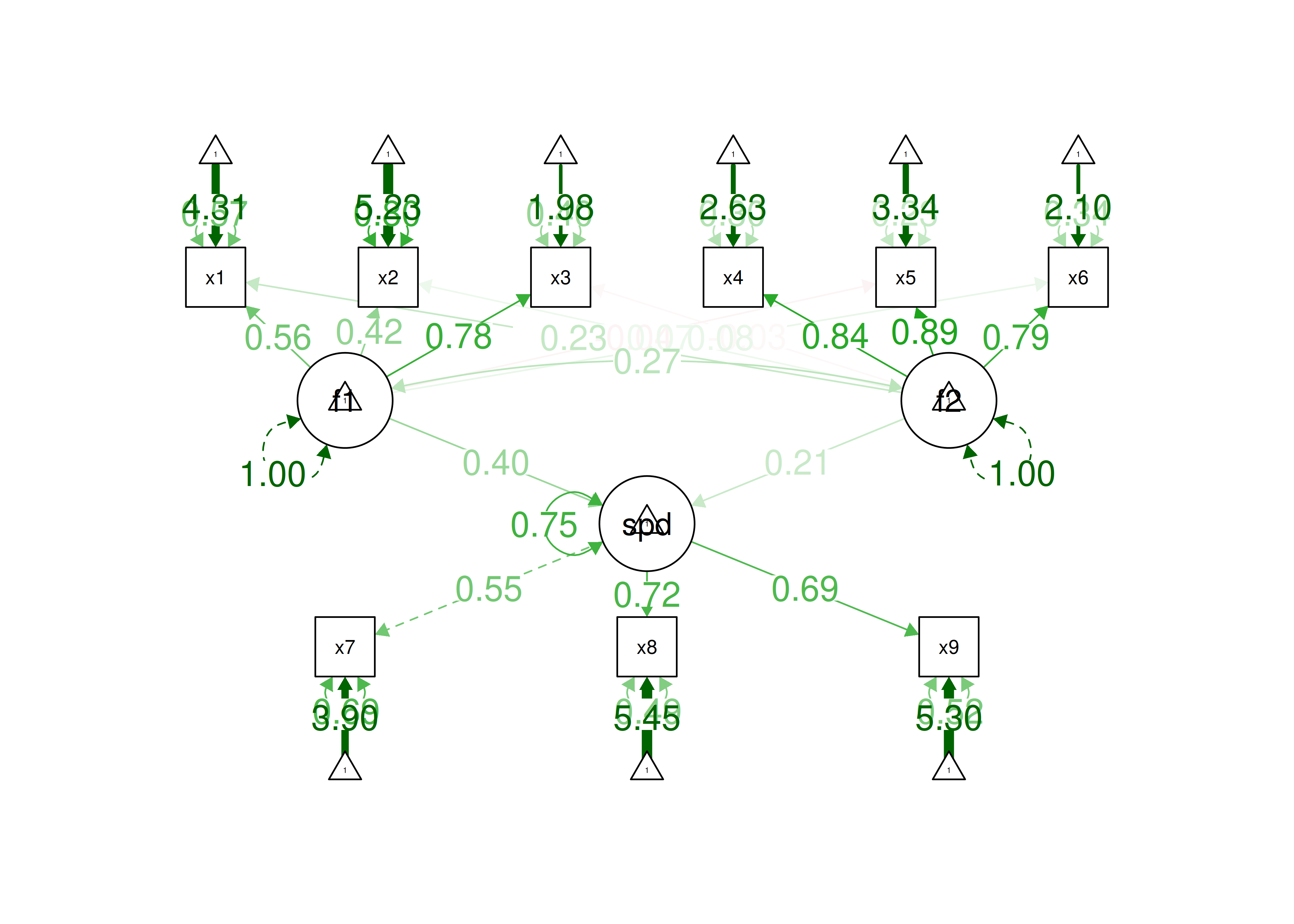
Figure 14.89: Exploratory Structural Equation Model With Exploratory Factors, Confirmatory Factors, and Regression Paths.
14.4.3.2.10 Equivalently fitting models
Markov equivalent directed acyclic graphs (DAGs) were depicted using the dagitty package (Textor et al., 2021).
Path diagrams of equivalent models are below.
Figure 14.90: Equivalently Fitting Models to an Exploratory Structural Equation Model.
Figure 14.91: Equivalently Fitting Models to an Exploratory Structural Equation Model.
Figure 14.92: Equivalently Fitting Models to an Exploratory Structural Equation Model.
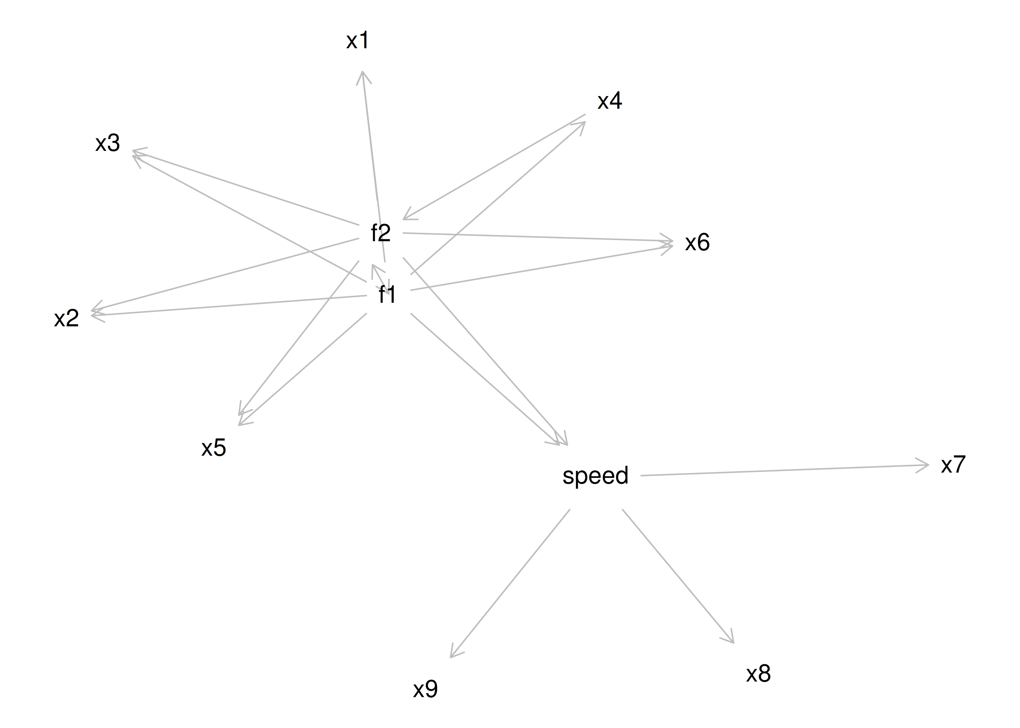
Figure 14.93: Equivalently Fitting Models to an Exploratory Structural Equation Model.
[[1]]
[[1]]$mar
[1] 0 0 0 0
[[2]]
[[2]]$mar
[1] 0 0 0 0
[[3]]
[[3]]$mar
[1] 0 0 0 0
[[4]]
[[4]]$mar
[1] 0 0 0 014.5 Principal Component Analysis (PCA)
Principal component analysis (PCA) is a technique for data reduction. PCA seeks to identify the principal components of the data, so that data can be reduced to that smaller set of components. That is, PCA seeks to identify the smallest set of components that explain the most variance in the variables. Although PCA is sometimes referred to as factor analysis, PCA is not factor analysis (Lilienfeld et al., 2015). PCA uses the total variance of all variables, whereas factor analysis uses the common variance among the variables.
14.5.1 Determine number of components
Determine the number of components to retain using the Scree plot and Very Simple Structure (VSS) plot.
14.5.1.1 Scree Plot
Scree plots were generated using the psych (Revelle, 2022) and nFactors (Raiche & Magis, 2020) packages. Note that eigenvalues of factors in PCA models are higher than factors from EFA models, because PCA components include common variance among the indicators in addition to error variance, whereas EFA factors include only the common variance among the indicators. A scree plot based on parallel analysis is in Figure 14.94.
The number of components to keep would depend on which criteria one uses. Based on the rule to keep components whose eigenvalues are greater than 1 and based on the parallel test, we would keep three factors. However, based on the Cattell scree test (as operationalized by the optimal coordinates and acceleration factor), we would keep one or three factors. Therefore, interpretability of the factors would be important for deciding between whether to keep one, two, or three factors.
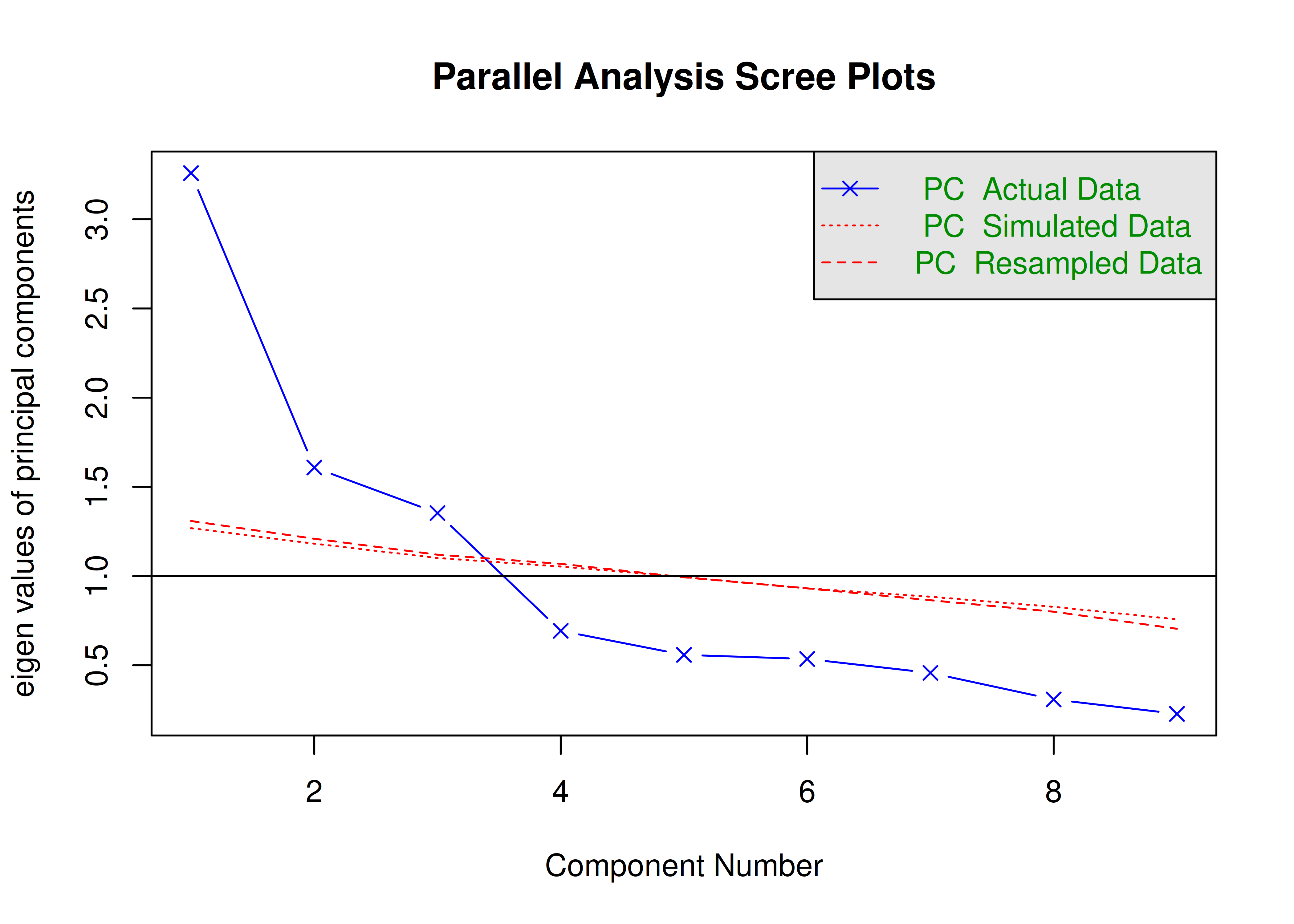
Figure 14.94: Scree Plot Based on Parallel Analysis in Principal Component Analysis.
Parallel analysis suggests that the number of factors = NA and the number of components = 3 A scree plot is in Figure 14.95.
Code
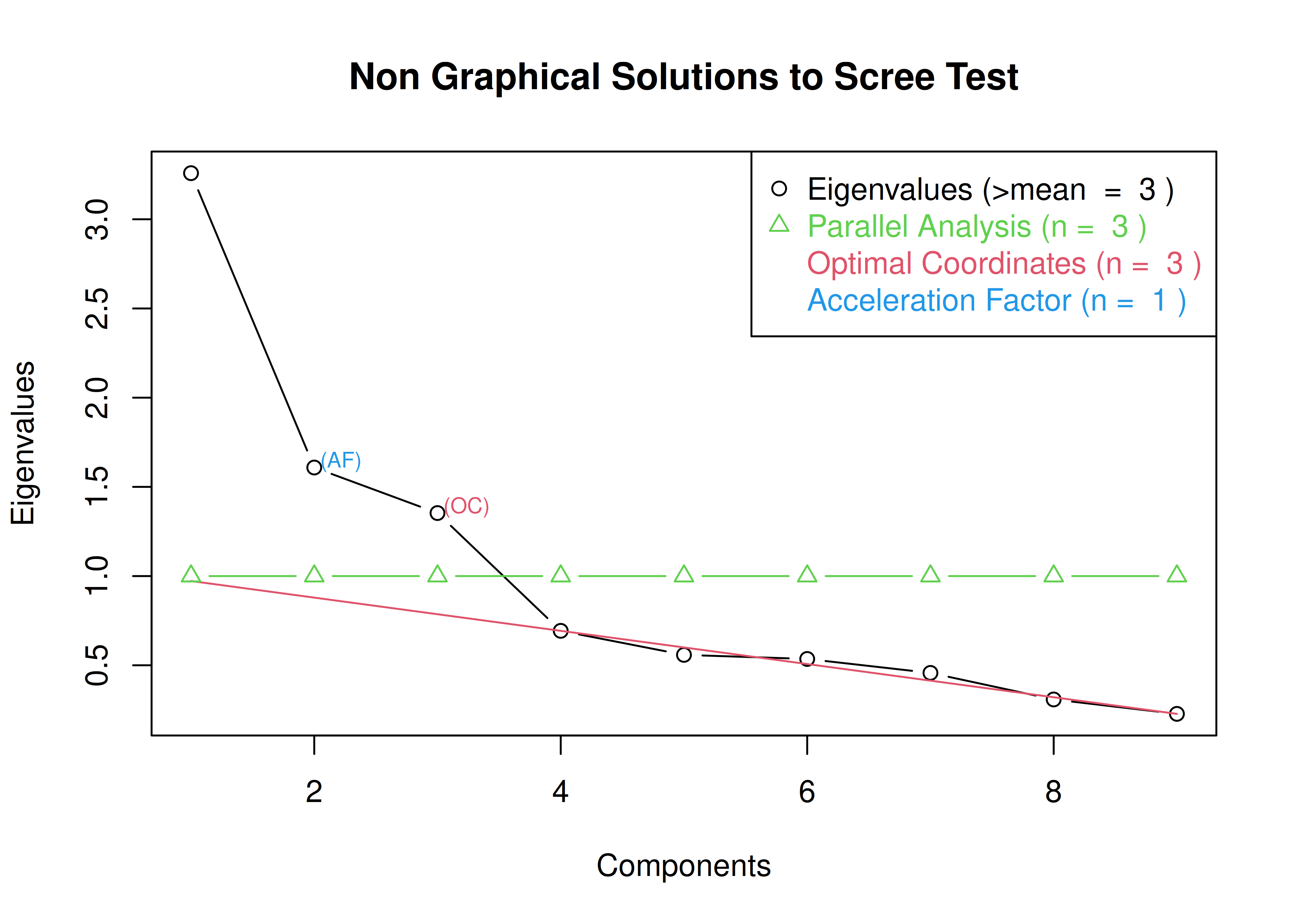
Figure 14.95: Scree Plot in Principal Component Analysis.
14.5.1.2 Very Simple Structure (VSS) Plot
Very simple structure (VSS) plots were generated using the psych package (Revelle, 2022).
14.5.1.2.1 Orthogonal (Varimax) rotation
In the example with orthogonal rotation below, the very simple structure (VSS) criterion is highest with three or four components.
A VSS plot of PCA with orthogonal rotation is in Figure 14.96.

Figure 14.96: Very Simple Structure Plot With Orthogonal Rotation in Principal Component Analysis.
Very Simple Structure
Call: vss(x = HolzingerSwineford1939[, vars], rotate = "varimax", fm = "pc")
VSS complexity 1 achieves a maximimum of 0.75 with 4 factors
VSS complexity 2 achieves a maximimum of 0.91 with 4 factors
The Velicer MAP achieves a minimum of 0.07 with 2 factors
BIC achieves a minimum of Inf with factorsSample Size adjusted BIC achieves a minimum of Inf with factors
Statistics by number of factors
vss1 vss2 map dof chisq prob sqresid fit RMSEA BIC SABIC complex eChisq
1 0.64 0.00 0.078 0 NA NA 5.853 0.64 NA NA NA NA NA
2 0.69 0.80 0.067 0 NA NA 3.266 0.80 NA NA NA NA NA
3 0.74 0.88 0.071 0 NA NA 1.434 0.91 NA NA NA NA NA
4 0.75 0.91 0.125 0 NA NA 0.954 0.94 NA NA NA NA NA
5 0.71 0.87 0.199 0 NA NA 0.643 0.96 NA NA NA NA NA
6 0.71 0.85 0.403 0 NA NA 0.356 0.98 NA NA NA NA NA
7 0.71 0.84 0.447 0 NA NA 0.147 0.99 NA NA NA NA NA
8 0.59 0.82 1.000 0 NA NA 0.052 1.00 NA NA NA NA NA
SRMR eCRMS eBIC
1 NA NA NA
2 NA NA NA
3 NA NA NA
4 NA NA NA
5 NA NA NA
6 NA NA NA
7 NA NA NA
8 NA NA NA14.5.1.2.2 Oblique (Oblimin) rotation
In the example with orthogonal rotation below, the VSS criterion is highest with 2 components.
A VSS plot of PCA with oblique rotation is in Figure 14.97.
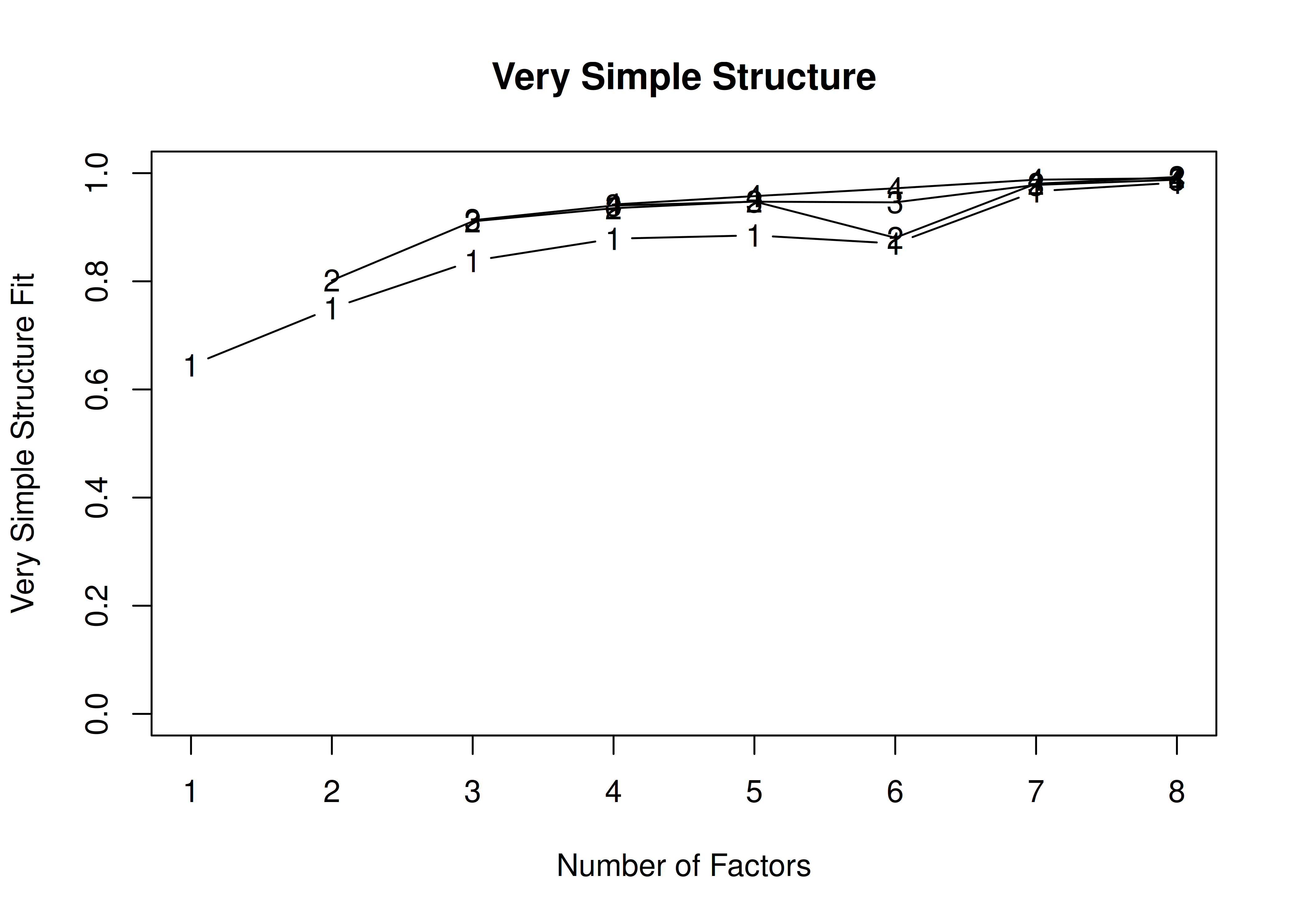
Figure 14.97: Very Simple Structure Plot With Oblique Rotation in Principal Component Analysis.
Very Simple Structure
Call: vss(x = HolzingerSwineford1939[, vars], rotate = "oblimin", fm = "pc")
VSS complexity 1 achieves a maximimum of 0.98 with 5 factors
VSS complexity 2 achieves a maximimum of 0.99 with 5 factors
The Velicer MAP achieves a minimum of 0.07 with 2 factors
BIC achieves a minimum of Inf with factorsSample Size adjusted BIC achieves a minimum of Inf with factors
Statistics by number of factors
vss1 vss2 map dof chisq prob sqresid fit RMSEA BIC SABIC complex eChisq
1 0.64 0.00 0.078 0 NA NA 5.853 0.64 NA NA NA NA NA
2 0.75 0.80 0.067 0 NA NA 3.266 0.80 NA NA NA NA NA
3 0.84 0.91 0.071 0 NA NA 1.434 0.91 NA NA NA NA NA
4 0.88 0.94 0.125 0 NA NA 0.954 0.94 NA NA NA NA NA
5 0.88 0.95 0.199 0 NA NA 0.643 0.96 NA NA NA NA NA
6 0.87 0.88 0.403 0 NA NA 0.356 0.98 NA NA NA NA NA
7 0.97 0.98 0.447 0 NA NA 0.147 0.99 NA NA NA NA NA
8 0.98 0.99 1.000 0 NA NA 0.052 1.00 NA NA NA NA NA
SRMR eCRMS eBIC
1 NA NA NA
2 NA NA NA
3 NA NA NA
4 NA NA NA
5 NA NA NA
6 NA NA NA
7 NA NA NA
8 NA NA NA14.5.1.2.3 No rotation
In the example with no rotation below, the VSS criterion is highest with 3 or 4 components.
A VSS plot of PCA with no rotation is in Figure 14.98.
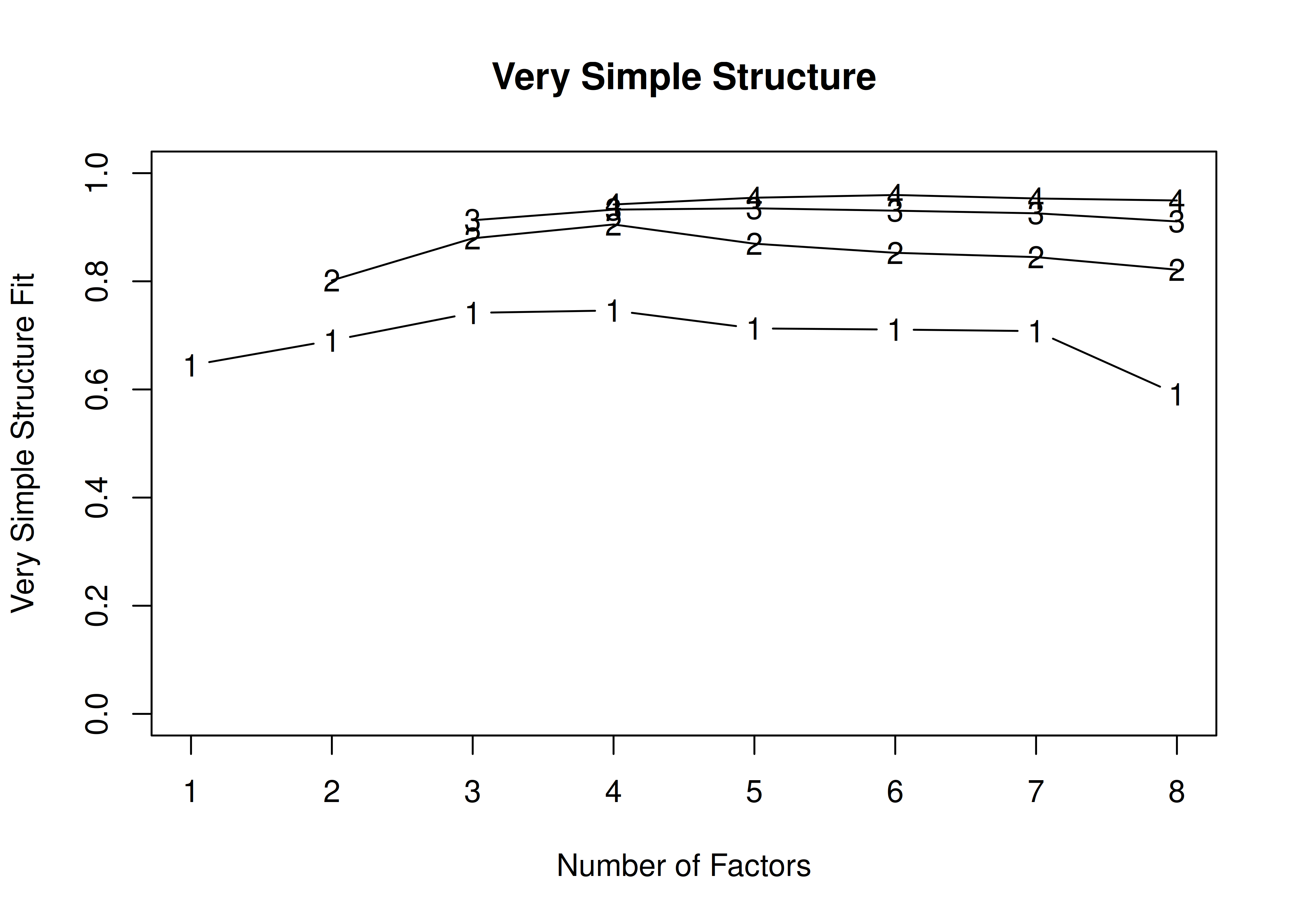
Figure 14.98: Very Simple Structure Plot With No Rotation in Principal Component Analysis.
Very Simple Structure
Call: vss(x = HolzingerSwineford1939[, vars], rotate = "none", fm = "pc")
VSS complexity 1 achieves a maximimum of 0.75 with 4 factors
VSS complexity 2 achieves a maximimum of 0.91 with 4 factors
The Velicer MAP achieves a minimum of 0.07 with 2 factors
BIC achieves a minimum of Inf with factorsSample Size adjusted BIC achieves a minimum of Inf with factors
Statistics by number of factors
vss1 vss2 map dof chisq prob sqresid fit RMSEA BIC SABIC complex eChisq
1 0.64 0.00 0.078 0 NA NA 5.853 0.64 NA NA NA NA NA
2 0.69 0.80 0.067 0 NA NA 3.266 0.80 NA NA NA NA NA
3 0.74 0.88 0.071 0 NA NA 1.434 0.91 NA NA NA NA NA
4 0.75 0.91 0.125 0 NA NA 0.954 0.94 NA NA NA NA NA
5 0.71 0.87 0.199 0 NA NA 0.643 0.96 NA NA NA NA NA
6 0.71 0.85 0.403 0 NA NA 0.356 0.98 NA NA NA NA NA
7 0.71 0.84 0.447 0 NA NA 0.147 0.99 NA NA NA NA NA
8 0.59 0.82 1.000 0 NA NA 0.052 1.00 NA NA NA NA NA
SRMR eCRMS eBIC
1 NA NA NA
2 NA NA NA
3 NA NA NA
4 NA NA NA
5 NA NA NA
6 NA NA NA
7 NA NA NA
8 NA NA NA14.5.2 Run the Principal Component Analysis
Principal component analysis (PCA) models were fit using the psych package (Revelle, 2022).
14.5.2.1 Orthogonal (Varimax) rotation
Code
pca1factorOrthogonal <- principal(
HolzingerSwineford1939[,vars],
nfactors = 1,
rotate = "varimax")
pca2factorOrthogonal <- principal(
HolzingerSwineford1939[,vars],
nfactors = 2,
rotate = "varimax")
pca3factorOrthogonal <- principal(
HolzingerSwineford1939[,vars],
nfactors = 3,
rotate = "varimax")
pca4factorOrthogonal <- principal(
HolzingerSwineford1939[,vars],
nfactors = 4,
rotate = "varimax")
pca5factorOrthogonal <- principal(
HolzingerSwineford1939[,vars],
nfactors = 5,
rotate = "varimax")
pca6factorOrthogonal <- principal(
HolzingerSwineford1939[,vars],
nfactors = 6,
rotate = "varimax")
pca7factorOrthogonal <- principal(
HolzingerSwineford1939[,vars],
nfactors = 7,
rotate = "varimax")
pca8factorOrthogonal <- principal(
HolzingerSwineford1939[,vars],
nfactors = 8,
rotate = "varimax")
pca9factorOrthogonal <- principal(
HolzingerSwineford1939[,vars],
nfactors = 9,
rotate = "varimax")14.5.2.2 Oblique (Oblimin) rotation
Code
pca1factorOblique <- principal(
HolzingerSwineford1939[,vars],
nfactors = 1,
rotate = "oblimin")
pca2factorOblique <- principal(
HolzingerSwineford1939[,vars],
nfactors = 2,
rotate = "oblimin")
pca3factorOblique <- principal(
HolzingerSwineford1939[,vars],
nfactors = 3,
rotate = "oblimin")
pca4factorOblique <- principal(
HolzingerSwineford1939[,vars],
nfactors = 4,
rotate = "oblimin")
pca5factorOblique <- principal(
HolzingerSwineford1939[,vars],
nfactors = 5,
rotate = "oblimin")
pca6factorOblique <- principal(
HolzingerSwineford1939[,vars],
nfactors = 6,
rotate = "oblimin")
pca7factorOblique <- principal(
HolzingerSwineford1939[,vars],
nfactors = 7,
rotate = "oblimin")
pca8factorOblique <- principal(
HolzingerSwineford1939[,vars],
nfactors = 8,
rotate = "oblimin")
pca9factorOblique <- principal(
HolzingerSwineford1939[,vars],
nfactors = 9,
rotate = "oblimin")14.5.3 Component Loadings
14.5.3.1 Orthogonal (Varimax) rotation
Principal Components Analysis
Call: principal(r = HolzingerSwineford1939[, vars], nfactors = 1, rotate = "varimax")
Standardized loadings (pattern matrix) based upon correlation matrix
PC1 h2 u2 com
x1 0.66 0.43 0.57 1
x2 0.40 0.16 0.84 1
x3 0.53 0.28 0.72 1
x4 0.75 0.56 0.44 1
x5 0.76 0.57 0.43 1
x6 0.73 0.53 0.47 1
x7 0.33 0.11 0.89 1
x8 0.51 0.26 0.74 1
x9 0.59 0.35 0.65 1
PC1
SS loadings 3.26
Proportion Var 0.36
Mean item complexity = 1
Test of the hypothesis that 1 component is sufficient.
The root mean square of the residuals (RMSR) is 0.16
with the empirical chi square 586.74 with prob < 1.7e-106
Fit based upon off diagonal values = 0.74Principal Components Analysis
Call: principal(r = HolzingerSwineford1939[, vars], nfactors = 2, rotate = "varimax")
Standardized loadings (pattern matrix) based upon correlation matrix
RC1 RC2 h2 u2 com
x1 0.51 0.42 0.43 0.57 1.9
x2 0.32 0.23 0.16 0.84 1.8
x3 0.27 0.54 0.36 0.64 1.5
x4 0.88 0.06 0.77 0.23 1.0
x5 0.86 0.09 0.75 0.25 1.0
x6 0.85 0.06 0.73 0.27 1.0
x7 -0.05 0.65 0.42 0.58 1.0
x8 0.08 0.77 0.60 0.40 1.0
x9 0.18 0.77 0.63 0.37 1.1
RC1 RC2
SS loadings 2.71 2.15
Proportion Var 0.30 0.24
Cumulative Var 0.30 0.54
Proportion Explained 0.56 0.44
Cumulative Proportion 0.56 1.00
Mean item complexity = 1.3
Test of the hypothesis that 2 components are sufficient.
The root mean square of the residuals (RMSR) is 0.12
with the empirical chi square 306.64 with prob < 8.7e-54
Fit based upon off diagonal values = 0.86Principal Components Analysis
Call: principal(r = HolzingerSwineford1939[, vars], nfactors = 3, rotate = "varimax")
Standardized loadings (pattern matrix) based upon correlation matrix
RC1 RC3 RC2 h2 u2 com
x1 0.32 0.68 0.15 0.59 0.41 1.5
x2 0.09 0.73 -0.12 0.55 0.45 1.1
x3 0.04 0.78 0.20 0.64 0.36 1.1
x4 0.89 0.13 0.08 0.82 0.18 1.1
x5 0.88 0.12 0.11 0.81 0.19 1.1
x6 0.86 0.13 0.07 0.77 0.23 1.1
x7 0.08 -0.16 0.83 0.73 0.27 1.1
x8 0.10 0.15 0.81 0.68 0.32 1.1
x9 0.10 0.45 0.65 0.63 0.37 1.8
RC1 RC3 RC2
SS loadings 2.46 1.90 1.87
Proportion Var 0.27 0.21 0.21
Cumulative Var 0.27 0.48 0.69
Proportion Explained 0.39 0.31 0.30
Cumulative Proportion 0.39 0.70 1.00
Mean item complexity = 1.2
Test of the hypothesis that 3 components are sufficient.
The root mean square of the residuals (RMSR) is 0.08
with the empirical chi square 151.71 with prob < 2.5e-26
Fit based upon off diagonal values = 0.93Principal Components Analysis
Call: principal(r = HolzingerSwineford1939[, vars], nfactors = 4, rotate = "varimax")
Standardized loadings (pattern matrix) based upon correlation matrix
RC1 RC2 RC3 RC4 h2 u2 com
x1 0.31 0.06 0.77 0.09 0.70 0.296 1.4
x2 0.11 0.00 0.22 0.96 0.97 0.028 1.1
x3 0.03 0.11 0.84 0.16 0.75 0.255 1.1
x4 0.89 0.06 0.18 -0.02 0.82 0.178 1.1
x5 0.88 0.13 0.07 0.12 0.82 0.181 1.1
x6 0.86 0.07 0.12 0.06 0.77 0.229 1.1
x7 0.07 0.83 -0.06 -0.17 0.73 0.267 1.1
x8 0.10 0.82 0.14 0.11 0.72 0.284 1.1
x9 0.09 0.62 0.47 0.14 0.63 0.368 2.0
RC1 RC2 RC3 RC4
SS loadings 2.45 1.80 1.64 1.02
Proportion Var 0.27 0.20 0.18 0.11
Cumulative Var 0.27 0.47 0.65 0.77
Proportion Explained 0.35 0.26 0.24 0.15
Cumulative Proportion 0.35 0.61 0.85 1.00
Mean item complexity = 1.2
Test of the hypothesis that 4 components are sufficient.
The root mean square of the residuals (RMSR) is 0.07
with the empirical chi square 119.21 with prob < 2.4e-23
Fit based upon off diagonal values = 0.95Principal Components Analysis
Call: principal(r = HolzingerSwineford1939[, vars], nfactors = 5, rotate = "varimax")
Standardized loadings (pattern matrix) based upon correlation matrix
RC1 RC2 RC3 RC4 RC5 h2 u2 com
x1 0.26 0.08 0.29 0.13 0.87 0.94 0.063 1.5
x2 0.11 -0.02 0.18 0.96 0.11 0.97 0.027 1.1
x3 0.08 0.01 0.87 0.15 0.26 0.86 0.144 1.3
x4 0.88 0.05 0.08 -0.02 0.18 0.82 0.178 1.1
x5 0.89 0.12 0.06 0.12 0.04 0.83 0.173 1.1
x6 0.87 0.06 0.07 0.06 0.09 0.77 0.225 1.1
x7 0.09 0.82 0.11 -0.17 -0.15 0.74 0.259 1.2
x8 0.07 0.85 0.01 0.13 0.29 0.83 0.171 1.3
x9 0.14 0.54 0.62 0.12 0.03 0.71 0.288 2.2
RC1 RC2 RC3 RC4 RC5
SS loadings 2.44 1.72 1.29 1.03 0.99
Proportion Var 0.27 0.19 0.14 0.11 0.11
Cumulative Var 0.27 0.46 0.61 0.72 0.83
Proportion Explained 0.33 0.23 0.17 0.14 0.13
Cumulative Proportion 0.33 0.56 0.73 0.87 1.00
Mean item complexity = 1.3
Test of the hypothesis that 5 components are sufficient.
The root mean square of the residuals (RMSR) is 0.07
with the empirical chi square 98 with prob < 4.2e-23
Fit based upon off diagonal values = 0.96Principal Components Analysis
Call: principal(r = HolzingerSwineford1939[, vars], nfactors = 6, rotate = "varimax")
Standardized loadings (pattern matrix) based upon correlation matrix
RC1 RC2 RC6 RC5 RC4 RC3 h2 u2 com
x1 0.26 0.00 0.12 0.87 0.13 0.28 0.94 0.062 1.5
x2 0.11 -0.05 0.07 0.11 0.97 0.16 0.99 0.010 1.1
x3 0.08 0.06 0.21 0.24 0.19 0.88 0.91 0.086 1.4
x4 0.88 0.08 -0.02 0.18 0.00 0.10 0.83 0.169 1.1
x5 0.89 0.02 0.20 0.05 0.10 -0.03 0.85 0.153 1.1
x6 0.87 0.06 0.04 0.09 0.07 0.07 0.78 0.224 1.1
x7 0.09 0.94 0.09 -0.09 -0.09 0.13 0.93 0.066 1.1
x8 0.07 0.64 0.49 0.37 0.12 -0.19 0.84 0.158 2.9
x9 0.13 0.19 0.90 0.08 0.06 0.26 0.94 0.064 1.3
RC1 RC2 RC6 RC5 RC4 RC3
SS loadings 2.44 1.35 1.15 1.03 1.02 1.01
Proportion Var 0.27 0.15 0.13 0.11 0.11 0.11
Cumulative Var 0.27 0.42 0.55 0.66 0.78 0.89
Proportion Explained 0.31 0.17 0.14 0.13 0.13 0.13
Cumulative Proportion 0.31 0.47 0.62 0.75 0.87 1.00
Mean item complexity = 1.4
Test of the hypothesis that 6 components are sufficient.
The root mean square of the residuals (RMSR) is 0.05
with the empirical chi square 62.84 with prob < NA
Fit based upon off diagonal values = 0.97Principal Components Analysis
Call: principal(r = HolzingerSwineford1939[, vars], nfactors = 7, rotate = "varimax")
Standardized loadings (pattern matrix) based upon correlation matrix
RC1 RC2 RC3 RC4 RC7 RC6 RC5 h2 u2 com
x1 0.23 -0.02 0.22 0.14 0.12 0.13 0.91 0.98 0.01620 1.4
x2 0.10 -0.06 0.15 0.97 0.03 0.07 0.12 1.00 0.00079 1.1
x3 0.09 0.03 0.94 0.16 0.06 0.18 0.20 0.99 0.01059 1.3
x4 0.86 0.16 0.01 0.03 -0.10 0.05 0.27 0.86 0.14081 1.3
x5 0.89 -0.01 -0.02 0.10 0.09 0.18 0.05 0.85 0.15266 1.1
x6 0.88 -0.01 0.15 0.04 0.15 -0.03 0.04 0.83 0.17414 1.1
x7 0.07 0.95 0.03 -0.06 0.24 0.15 -0.01 0.99 0.01101 1.2
x8 0.10 0.26 0.06 0.03 0.92 0.21 0.11 0.98 0.01810 1.3
x9 0.12 0.16 0.19 0.08 0.21 0.92 0.13 0.99 0.01167 1.4
RC1 RC2 RC3 RC4 RC7 RC6 RC5
SS loadings 2.42 1.03 1.01 1.01 1.00 1.00 0.99
Proportion Var 0.27 0.11 0.11 0.11 0.11 0.11 0.11
Cumulative Var 0.27 0.38 0.50 0.61 0.72 0.83 0.94
Proportion Explained 0.29 0.12 0.12 0.12 0.12 0.12 0.12
Cumulative Proportion 0.29 0.41 0.53 0.65 0.76 0.88 1.00
Mean item complexity = 1.3
Test of the hypothesis that 7 components are sufficient.
The root mean square of the residuals (RMSR) is 0.03
with the empirical chi square 21.82 with prob < NA
Fit based upon off diagonal values = 0.99Principal Components Analysis
Call: principal(r = HolzingerSwineford1939[, vars], nfactors = 8, rotate = "varimax")
Standardized loadings (pattern matrix) based upon correlation matrix
RC1 RC2 RC4 RC3 RC7 RC5 RC6 RC8 h2 u2 com
x1 0.21 -0.01 0.14 0.22 0.11 0.92 0.14 0.07 0.99 1.1e-02 1.4
x2 0.09 -0.06 0.97 0.15 0.03 0.12 0.07 0.04 1.00 5.2e-04 1.1
x3 0.07 0.03 0.16 0.95 0.07 0.20 0.17 0.05 1.00 1.0e-05 1.2
x4 0.89 0.14 0.03 0.06 -0.05 0.25 0.01 0.13 0.90 1.0e-01 1.3
x5 0.91 -0.04 0.09 0.03 0.15 0.02 0.14 0.15 0.91 9.3e-02 1.2
x6 0.61 0.03 0.06 0.08 0.07 0.11 0.04 0.77 1.00 5.4e-05 2.0
x7 0.07 0.95 -0.06 0.03 0.23 -0.01 0.15 0.02 0.99 8.2e-03 1.2
x8 0.08 0.26 0.03 0.07 0.93 0.11 0.20 0.05 0.99 7.7e-03 1.3
x9 0.12 0.17 0.08 0.18 0.21 0.13 0.92 0.03 1.00 2.6e-03 1.4
RC1 RC2 RC4 RC3 RC7 RC5 RC6 RC8
SS loadings 2.08 1.02 1.01 1.01 1.00 1.00 0.99 0.65
Proportion Var 0.23 0.11 0.11 0.11 0.11 0.11 0.11 0.07
Cumulative Var 0.23 0.35 0.46 0.57 0.68 0.79 0.90 0.97
Proportion Explained 0.24 0.12 0.12 0.12 0.11 0.11 0.11 0.07
Cumulative Proportion 0.24 0.35 0.47 0.58 0.70 0.81 0.93 1.00
Mean item complexity = 1.3
Test of the hypothesis that 8 components are sufficient.
The root mean square of the residuals (RMSR) is 0.02
with the empirical chi square 9.61 with prob < NA
Fit based upon off diagonal values = 1Principal Components Analysis
Call: principal(r = HolzingerSwineford1939[, vars], nfactors = 9, rotate = "varimax")
Standardized loadings (pattern matrix) based upon correlation matrix
RC8 RC2 RC4 RC3 RC5 RC7 RC6 RC1 RC9 h2 u2 com
x1 0.11 -0.01 0.14 0.22 0.93 0.11 0.13 0.09 0.15 1 -1.1e-15 1.3
x2 0.05 -0.06 0.97 0.15 0.12 0.03 0.07 0.06 0.04 1 -4.4e-16 1.1
x3 0.06 0.03 0.16 0.95 0.20 0.07 0.17 0.03 0.04 1 -8.9e-16 1.2
x4 0.34 0.08 0.05 0.05 0.19 0.01 0.05 0.36 0.84 1 0.0e+00 1.9
x5 0.35 0.03 0.08 0.03 0.10 0.09 0.11 0.86 0.32 1 -1.3e-15 1.8
x6 0.90 0.03 0.06 0.07 0.12 0.07 0.05 0.30 0.27 1 1.1e-16 1.5
x7 0.03 0.96 -0.06 0.03 -0.01 0.23 0.15 0.02 0.06 1 -2.2e-16 1.2
x8 0.06 0.25 0.03 0.07 0.10 0.93 0.20 0.07 0.02 1 5.6e-16 1.3
x9 0.05 0.16 0.08 0.18 0.13 0.21 0.93 0.09 0.05 1 -6.7e-16 1.3
RC8 RC2 RC4 RC3 RC5 RC7 RC6 RC1 RC9
SS loadings 1.07 1.02 1.02 1.01 1.01 1.00 0.99 0.98 0.91
Proportion Var 0.12 0.11 0.11 0.11 0.11 0.11 0.11 0.11 0.10
Cumulative Var 0.12 0.23 0.34 0.46 0.57 0.68 0.79 0.90 1.00
Proportion Explained 0.12 0.11 0.11 0.11 0.11 0.11 0.11 0.11 0.10
Cumulative Proportion 0.12 0.23 0.34 0.46 0.57 0.68 0.79 0.90 1.00
Mean item complexity = 1.4
Test of the hypothesis that 9 components are sufficient.
The root mean square of the residuals (RMSR) is 0
with the empirical chi square 0 with prob < NA
Fit based upon off diagonal values = 114.5.3.2 Oblique (Oblimin) rotation
Principal Components Analysis
Call: principal(r = HolzingerSwineford1939[, vars], nfactors = 1, rotate = "oblimin")
Standardized loadings (pattern matrix) based upon correlation matrix
PC1 h2 u2 com
x1 0.66 0.43 0.57 1
x2 0.40 0.16 0.84 1
x3 0.53 0.28 0.72 1
x4 0.75 0.56 0.44 1
x5 0.76 0.57 0.43 1
x6 0.73 0.53 0.47 1
x7 0.33 0.11 0.89 1
x8 0.51 0.26 0.74 1
x9 0.59 0.35 0.65 1
PC1
SS loadings 3.26
Proportion Var 0.36
Mean item complexity = 1
Test of the hypothesis that 1 component is sufficient.
The root mean square of the residuals (RMSR) is 0.16
with the empirical chi square 586.74 with prob < 1.7e-106
Fit based upon off diagonal values = 0.74Principal Components Analysis
Call: principal(r = HolzingerSwineford1939[, vars], nfactors = 2, rotate = "oblimin")
Standardized loadings (pattern matrix) based upon correlation matrix
TC1 TC2 h2 u2 com
x1 0.45 0.39 0.43 0.57 2.0
x2 0.29 0.21 0.16 0.84 1.8
x3 0.19 0.53 0.36 0.64 1.2
x4 0.88 -0.02 0.77 0.23 1.0
x5 0.87 0.01 0.75 0.25 1.0
x6 0.86 -0.02 0.73 0.27 1.0
x7 -0.15 0.67 0.42 0.58 1.1
x8 -0.05 0.79 0.60 0.40 1.0
x9 0.06 0.78 0.63 0.37 1.0
TC1 TC2
SS loadings 2.67 2.20
Proportion Var 0.30 0.24
Cumulative Var 0.30 0.54
Proportion Explained 0.55 0.45
Cumulative Proportion 0.55 1.00
With component correlations of
TC1 TC2
TC1 1.00 0.25
TC2 0.25 1.00
Mean item complexity = 1.2
Test of the hypothesis that 2 components are sufficient.
The root mean square of the residuals (RMSR) is 0.12
with the empirical chi square 306.64 with prob < 8.7e-54
Fit based upon off diagonal values = 0.86Principal Components Analysis
Call: principal(r = HolzingerSwineford1939[, vars], nfactors = 3, rotate = "oblimin")
Standardized loadings (pattern matrix) based upon correlation matrix
TC1 TC3 TC2 h2 u2 com
x1 0.24 0.65 0.05 0.59 0.41 1.3
x2 0.02 0.74 -0.21 0.55 0.45 1.2
x3 -0.06 0.79 0.11 0.64 0.36 1.1
x4 0.90 0.00 -0.01 0.82 0.18 1.0
x5 0.89 -0.01 0.03 0.81 0.19 1.0
x6 0.88 0.01 -0.01 0.77 0.23 1.0
x7 0.03 -0.20 0.86 0.73 0.27 1.1
x8 0.02 0.12 0.79 0.68 0.32 1.0
x9 0.00 0.43 0.60 0.63 0.37 1.8
TC1 TC3 TC2
SS loadings 2.49 1.90 1.82
Proportion Var 0.28 0.21 0.20
Cumulative Var 0.28 0.49 0.69
Proportion Explained 0.40 0.31 0.29
Cumulative Proportion 0.40 0.71 1.00
With component correlations of
TC1 TC3 TC2
TC1 1.00 0.27 0.18
TC3 0.27 1.00 0.16
TC2 0.18 0.16 1.00
Mean item complexity = 1.2
Test of the hypothesis that 3 components are sufficient.
The root mean square of the residuals (RMSR) is 0.08
with the empirical chi square 151.71 with prob < 2.5e-26
Fit based upon off diagonal values = 0.93Principal Components Analysis
Call: principal(r = HolzingerSwineford1939[, vars], nfactors = 4, rotate = "oblimin")
Standardized loadings (pattern matrix) based upon correlation matrix
TC1 TC2 TC3 TC4 h2 u2 com
x1 0.21 -0.05 0.78 -0.03 0.70 0.296 1.2
x2 0.02 -0.01 0.00 0.98 0.97 0.028 1.0
x3 -0.10 0.02 0.86 0.05 0.75 0.255 1.0
x4 0.90 -0.03 0.09 -0.08 0.82 0.178 1.0
x5 0.89 0.06 -0.07 0.09 0.82 0.181 1.0
x6 0.87 0.00 0.00 0.02 0.77 0.229 1.0
x7 0.03 0.85 -0.11 -0.15 0.73 0.267 1.1
x8 0.02 0.82 0.03 0.11 0.72 0.284 1.0
x9 -0.02 0.58 0.41 0.09 0.63 0.368 1.9
TC1 TC2 TC3 TC4
SS loadings 2.46 1.79 1.61 1.06
Proportion Var 0.27 0.20 0.18 0.12
Cumulative Var 0.27 0.47 0.65 0.77
Proportion Explained 0.36 0.26 0.23 0.15
Cumulative Proportion 0.36 0.61 0.85 1.00
With component correlations of
TC1 TC2 TC3 TC4
TC1 1.00 0.18 0.28 0.17
TC2 0.18 1.00 0.21 0.03
TC3 0.28 0.21 1.00 0.36
TC4 0.17 0.03 0.36 1.00
Mean item complexity = 1.1
Test of the hypothesis that 4 components are sufficient.
The root mean square of the residuals (RMSR) is 0.07
with the empirical chi square 119.21 with prob < 2.4e-23
Fit based upon off diagonal values = 0.95Principal Components Analysis
Call: principal(r = HolzingerSwineford1939[, vars], nfactors = 5, rotate = "oblimin")
Standardized loadings (pattern matrix) based upon correlation matrix
TC1 TC2 TC3 TC4 TC5 h2 u2 com
x1 0.09 0.06 0.13 0.00 0.88 0.94 0.063 1.1
x2 0.02 -0.01 0.03 0.98 -0.02 0.97 0.027 1.0
x3 -0.02 -0.11 0.87 0.05 0.17 0.86 0.144 1.1
x4 0.89 -0.03 0.00 -0.08 0.11 0.82 0.178 1.1
x5 0.91 0.04 -0.02 0.08 -0.07 0.83 0.173 1.0
x6 0.88 -0.02 0.00 0.02 0.01 0.77 0.225 1.0
x7 0.08 0.79 0.12 -0.17 -0.21 0.74 0.259 1.3
x8 -0.04 0.88 -0.11 0.10 0.24 0.83 0.171 1.2
x9 0.06 0.45 0.60 0.08 -0.09 0.71 0.288 2.0
TC1 TC2 TC3 TC4 TC5
SS loadings 2.45 1.68 1.27 1.06 1.01
Proportion Var 0.27 0.19 0.14 0.12 0.11
Cumulative Var 0.27 0.46 0.60 0.72 0.83
Proportion Explained 0.33 0.22 0.17 0.14 0.14
Cumulative Proportion 0.33 0.55 0.72 0.86 1.00
With component correlations of
TC1 TC2 TC3 TC4 TC5
TC1 1.00 0.18 0.19 0.17 0.28
TC2 0.18 1.00 0.23 0.01 0.08
TC3 0.19 0.23 1.00 0.26 0.31
TC4 0.17 0.01 0.26 1.00 0.29
TC5 0.28 0.08 0.31 0.29 1.00
Mean item complexity = 1.2
Test of the hypothesis that 5 components are sufficient.
The root mean square of the residuals (RMSR) is 0.07
with the empirical chi square 98 with prob < 4.2e-23
Fit based upon off diagonal values = 0.96Principal Components Analysis
Call: principal(r = HolzingerSwineford1939[, vars], nfactors = 6, rotate = "oblimin")
Standardized loadings (pattern matrix) based upon correlation matrix
TC1 TC6 TC2 TC5 TC4 TC3 h2 u2 com
x1 0.08 -0.09 -0.03 0.93 0.01 0.10 0.94 0.062 1.1
x2 0.01 -0.02 -0.04 -0.02 1.00 0.02 0.99 0.010 1.0
x3 -0.03 0.11 0.21 0.20 0.12 0.78 0.91 0.086 1.4
x4 0.88 0.07 -0.10 0.12 -0.05 0.06 0.83 0.169 1.1
x5 0.90 -0.06 0.17 -0.06 0.05 -0.10 0.85 0.153 1.1
x6 0.87 0.04 -0.02 0.01 0.03 0.02 0.78 0.224 1.0
x7 0.05 0.99 -0.04 -0.09 -0.04 0.07 0.93 0.066 1.0
x8 -0.07 0.48 0.34 0.36 0.10 -0.39 0.84 0.158 3.9
x9 0.05 -0.02 0.97 -0.03 -0.02 0.09 0.94 0.064 1.0
TC1 TC6 TC2 TC5 TC4 TC3
SS loadings 2.39 1.29 1.23 1.17 1.07 0.85
Proportion Var 0.27 0.14 0.14 0.13 0.12 0.09
Cumulative Var 0.27 0.41 0.55 0.68 0.80 0.89
Proportion Explained 0.30 0.16 0.15 0.15 0.13 0.11
Cumulative Proportion 0.30 0.46 0.61 0.76 0.89 1.00
With component correlations of
TC1 TC6 TC2 TC5 TC4 TC3
TC1 1.00 0.11 0.18 0.31 0.18 0.08
TC6 0.11 1.00 0.39 0.16 -0.02 -0.07
TC2 0.18 0.39 1.00 0.36 0.23 0.10
TC5 0.31 0.16 0.36 1.00 0.30 0.22
TC4 0.18 -0.02 0.23 0.30 1.00 0.20
TC3 0.08 -0.07 0.10 0.22 0.20 1.00
Mean item complexity = 1.4
Test of the hypothesis that 6 components are sufficient.
The root mean square of the residuals (RMSR) is 0.05
with the empirical chi square 62.84 with prob < NA
Fit based upon off diagonal values = 0.97Principal Components Analysis
Call: principal(r = HolzingerSwineford1939[, vars], nfactors = 7, rotate = "oblimin")
Standardized loadings (pattern matrix) based upon correlation matrix
TC1 TC4 TC6 TC5 TC7 TC3 TC2 h2 u2 com
x1 0.00 0.02 -0.04 0.95 0.02 0.04 0.06 0.98 0.01620 1.0
x2 0.00 1.00 0.00 0.00 -0.01 0.00 0.00 1.00 0.00079 1.0
x3 0.01 0.02 0.02 0.03 0.04 0.97 -0.02 0.99 0.01059 1.0
x4 0.82 -0.01 0.18 0.23 0.00 -0.05 -0.19 0.86 0.14081 1.4
x5 0.90 0.06 -0.06 -0.05 0.16 -0.08 0.04 0.85 0.15266 1.1
x6 0.90 -0.01 -0.05 -0.06 -0.11 0.15 0.14 0.83 0.17414 1.2
x7 -0.01 0.00 0.97 -0.04 0.01 0.02 0.06 0.99 0.01101 1.0
x8 0.02 0.00 0.07 0.06 0.04 -0.02 0.93 0.98 0.01810 1.0
x9 0.01 0.00 0.01 0.01 0.96 0.04 0.02 0.99 0.01167 1.0
TC1 TC4 TC6 TC5 TC7 TC3 TC2
SS loadings 2.34 1.02 1.03 1.05 1.03 1.01 0.99
Proportion Var 0.26 0.11 0.11 0.12 0.11 0.11 0.11
Cumulative Var 0.26 0.37 0.49 0.60 0.72 0.83 0.94
Proportion Explained 0.28 0.12 0.12 0.12 0.12 0.12 0.12
Cumulative Proportion 0.28 0.40 0.52 0.64 0.76 0.88 1.00
With component correlations of
TC1 TC4 TC6 TC5 TC7 TC3 TC2
TC1 1.00 0.16 0.12 0.34 0.19 0.14 0.12
TC4 0.16 1.00 -0.09 0.28 0.20 0.32 0.08
TC6 0.12 -0.09 1.00 0.07 0.31 0.07 0.40
TC5 0.34 0.28 0.07 1.00 0.29 0.39 0.16
TC7 0.19 0.20 0.31 0.29 1.00 0.33 0.39
TC3 0.14 0.32 0.07 0.39 0.33 1.00 0.17
TC2 0.12 0.08 0.40 0.16 0.39 0.17 1.00
Mean item complexity = 1.1
Test of the hypothesis that 7 components are sufficient.
The root mean square of the residuals (RMSR) is 0.03
with the empirical chi square 21.82 with prob < NA
Fit based upon off diagonal values = 0.99Principal Components Analysis
Call: principal(r = HolzingerSwineford1939[, vars], nfactors = 8, rotate = "oblimin")
Standardized loadings (pattern matrix) based upon correlation matrix
TC1 TC8 TC3 TC4 TC2 TC6 TC7 TC5 h2 u2 com
x1 0.01 0.02 0.02 0.02 0.03 -0.03 0.04 0.95 0.99 1.1e-02 1.0
x2 0.00 0.00 0.00 1.00 0.00 0.01 -0.01 0.01 1.00 5.2e-04 1.0
x3 0.00 0.00 1.00 0.00 0.00 0.00 0.00 0.00 1.00 1.0e-05 1.0
x4 0.86 0.03 0.02 -0.02 -0.06 0.14 -0.12 0.18 0.90 1.0e-01 1.2
x5 0.90 0.05 0.00 0.04 0.08 -0.11 0.12 -0.11 0.91 9.3e-02 1.1
x6 0.00 1.00 0.00 0.00 0.00 0.00 0.00 0.00 1.00 5.4e-05 1.0
x7 0.00 0.01 0.00 0.00 0.03 0.97 0.04 -0.03 0.99 8.2e-03 1.0
x8 0.01 0.00 0.01 -0.01 0.00 0.04 0.97 0.04 0.99 7.7e-03 1.0
x9 0.00 0.00 0.00 0.00 0.99 0.02 -0.01 0.02 1.00 2.6e-03 1.0
TC1 TC8 TC3 TC4 TC2 TC6 TC7 TC5
SS loadings 1.64 1.07 1.02 1.01 1.02 1.01 1.01 1.01
Proportion Var 0.18 0.12 0.11 0.11 0.11 0.11 0.11 0.11
Cumulative Var 0.18 0.30 0.41 0.53 0.64 0.75 0.86 0.97
Proportion Explained 0.19 0.12 0.12 0.12 0.12 0.11 0.11 0.12
Cumulative Proportion 0.19 0.31 0.42 0.54 0.66 0.77 0.88 1.00
With component correlations of
TC1 TC8 TC3 TC4 TC2 TC6 TC7 TC5
TC1 1.00 0.71 0.14 0.16 0.21 0.11 0.14 0.32
TC8 0.71 1.00 0.20 0.17 0.18 0.09 0.17 0.30
TC3 0.14 0.20 1.00 0.34 0.39 0.08 0.18 0.43
TC4 0.16 0.17 0.34 1.00 0.20 -0.10 0.09 0.28
TC2 0.21 0.18 0.39 0.20 1.00 0.31 0.45 0.28
TC6 0.11 0.09 0.08 -0.10 0.31 1.00 0.43 0.05
TC7 0.14 0.17 0.18 0.09 0.45 0.43 1.00 0.19
TC5 0.32 0.30 0.43 0.28 0.28 0.05 0.19 1.00
Mean item complexity = 1
Test of the hypothesis that 8 components are sufficient.
The root mean square of the residuals (RMSR) is 0.02
with the empirical chi square 9.61 with prob < NA
Fit based upon off diagonal values = 1Principal Components Analysis
Call: principal(r = HolzingerSwineford1939[, vars], nfactors = 9, rotate = "oblimin")
Standardized loadings (pattern matrix) based upon correlation matrix
TC4 TC6 TC2 TC3 TC7 TC5 TC8 TC1 TC9 h2 u2 com
x1 0 0 0 0 0 1 0 0 0 1 -1.1e-15 1
x2 1 0 0 0 0 0 0 0 0 1 -4.4e-16 1
x3 0 0 0 1 0 0 0 0 0 1 -8.9e-16 1
x4 0 0 0 0 0 0 0 0 1 1 0.0e+00 1
x5 0 0 0 0 0 0 0 1 0 1 -1.3e-15 1
x6 0 0 0 0 0 0 1 0 0 1 1.1e-16 1
x7 0 1 0 0 0 0 0 0 0 1 -2.2e-16 1
x8 0 0 1 0 0 0 0 0 0 1 5.6e-16 1
x9 0 0 0 0 1 0 0 0 0 1 -6.7e-16 1
TC4 TC6 TC2 TC3 TC7 TC5 TC8 TC1 TC9
SS loadings 1.00 1.00 1.00 1.00 1.00 1.00 1.00 1.00 1.00
Proportion Var 0.11 0.11 0.11 0.11 0.11 0.11 0.11 0.11 0.11
Cumulative Var 0.11 0.22 0.33 0.44 0.56 0.67 0.78 0.89 1.00
Proportion Explained 0.11 0.11 0.11 0.11 0.11 0.11 0.11 0.11 0.11
Cumulative Proportion 0.11 0.22 0.33 0.44 0.56 0.67 0.78 0.89 1.00
With component correlations of
TC4 TC6 TC2 TC3 TC7 TC5 TC8 TC1 TC9
TC4 1.00 -0.09 0.09 0.34 0.20 0.32 0.17 0.19 0.15
TC6 -0.09 1.00 0.49 0.09 0.35 0.04 0.10 0.11 0.15
TC2 0.09 0.49 1.00 0.20 0.46 0.26 0.19 0.21 0.13
TC3 0.34 0.09 0.20 1.00 0.40 0.46 0.19 0.15 0.18
TC7 0.20 0.35 0.46 0.40 1.00 0.34 0.18 0.26 0.19
TC5 0.32 0.04 0.26 0.46 0.34 1.00 0.32 0.31 0.40
TC8 0.17 0.10 0.19 0.19 0.18 0.32 1.00 0.69 0.68
TC1 0.19 0.11 0.21 0.15 0.26 0.31 0.69 1.00 0.73
TC9 0.15 0.15 0.13 0.18 0.19 0.40 0.68 0.73 1.00
Mean item complexity = 1
Test of the hypothesis that 9 components are sufficient.
The root mean square of the residuals (RMSR) is 0
with the empirical chi square 0 with prob < NA
Fit based upon off diagonal values = 114.5.5 Plots
Biplots were generated using the psych package (Revelle, 2022).
Pairs panel plots were generated using the psych package (Revelle, 2022).
Correlation plots were generated using the corrplot package (Wei & Simko, 2021).
14.5.5.1 Biplot
A biplot is in Figure 14.99.
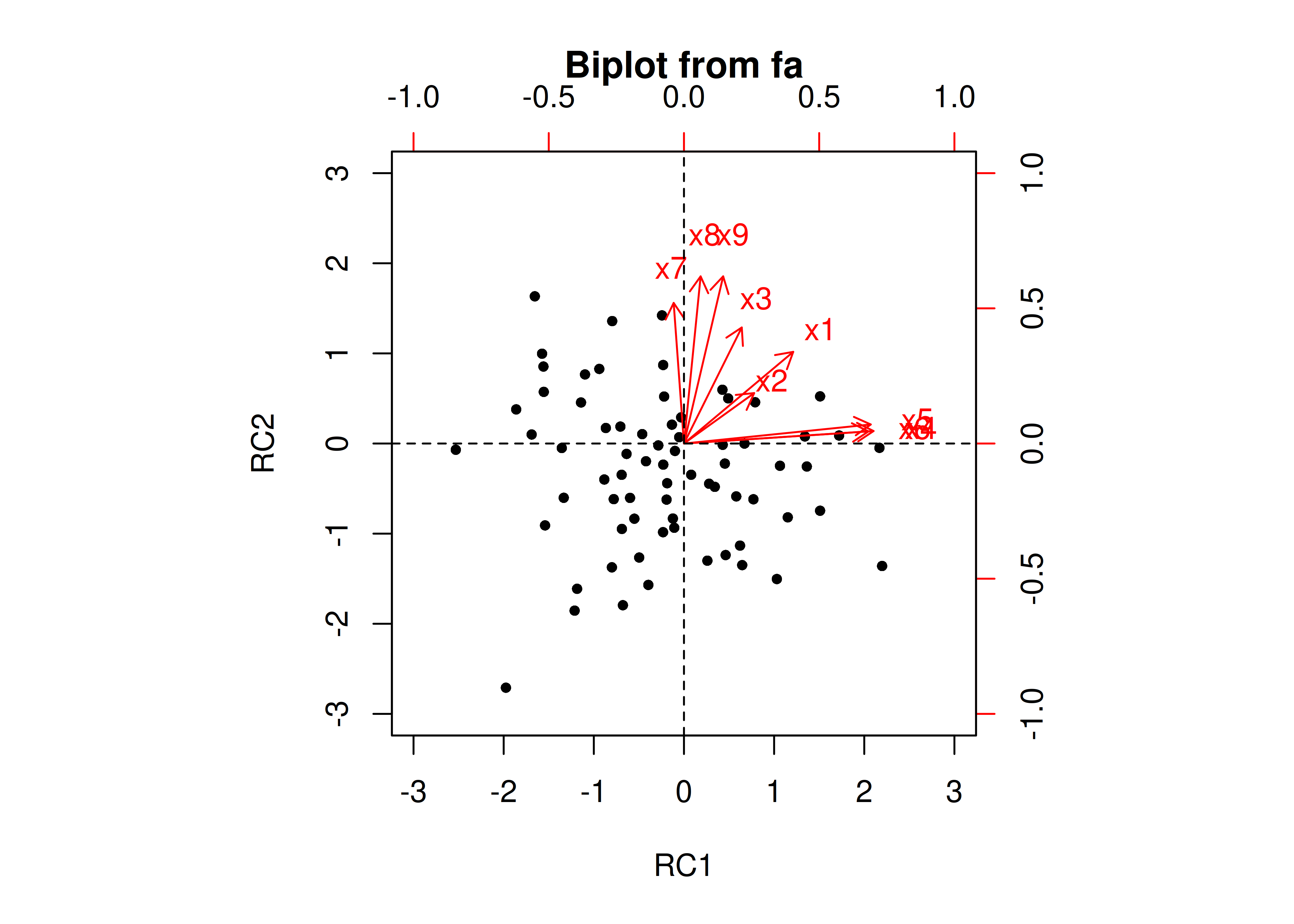
Figure 14.99: Biplot Using Orthogonal Rotation in Principal Component Analysis.
14.5.5.2 Orthogonal (Varimax) rotation
A pairs panel plot is in Figure 14.100.
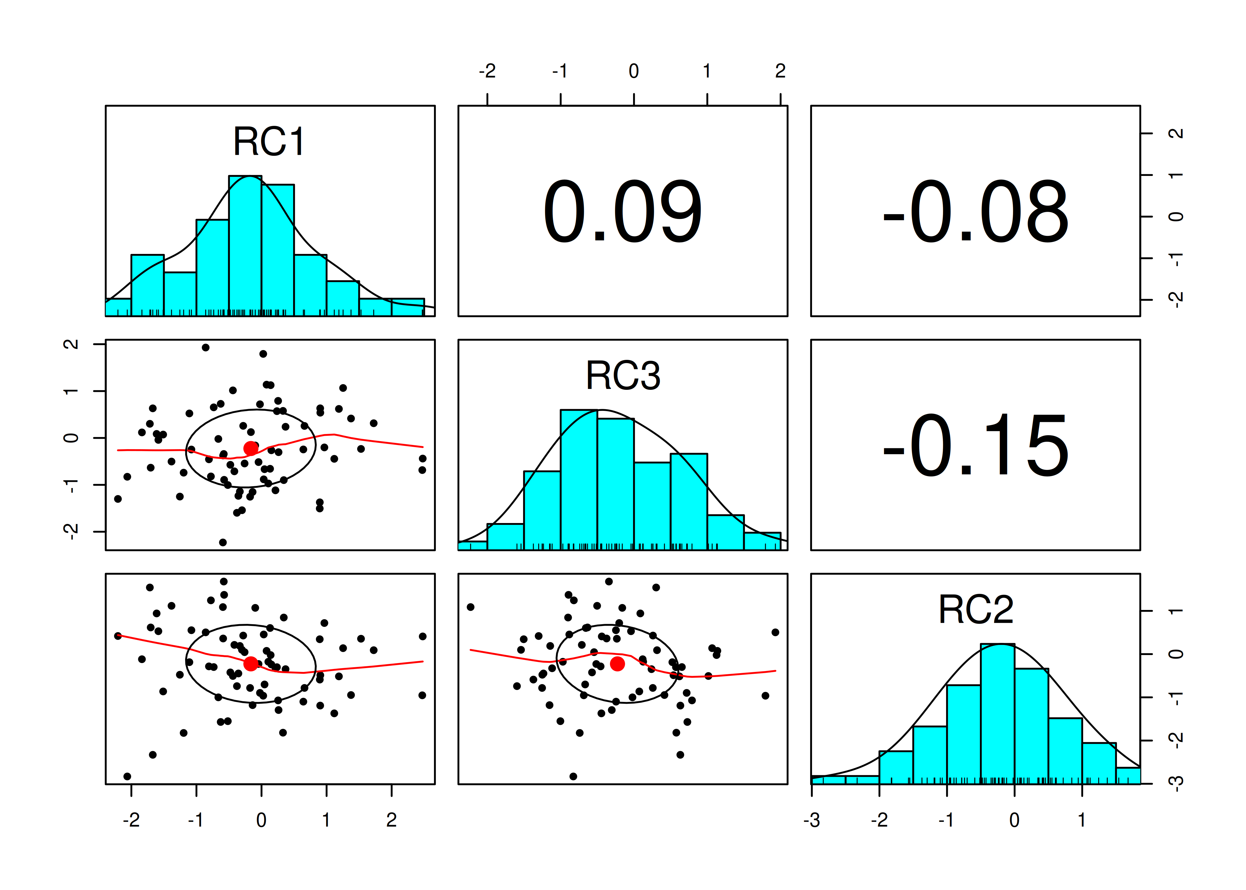
Figure 14.100: Pairs Panel Plot Using Orthogonal Rotation in Principal Component Analysis.
A correlation plot is in Figure 14.101.
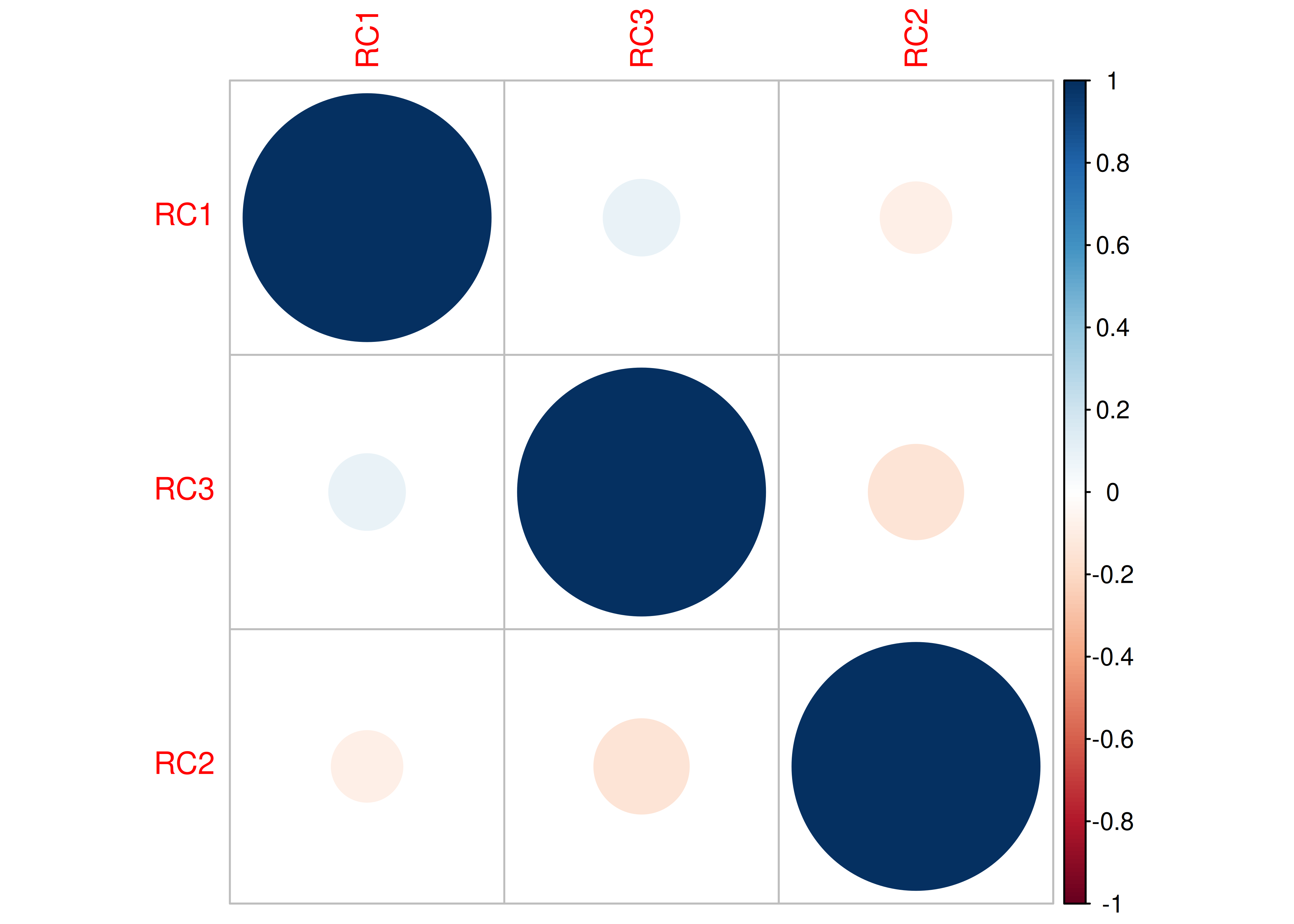
Figure 14.101: Correlation Plot Using Orthogonal Rotation in Principal Component Analysis.
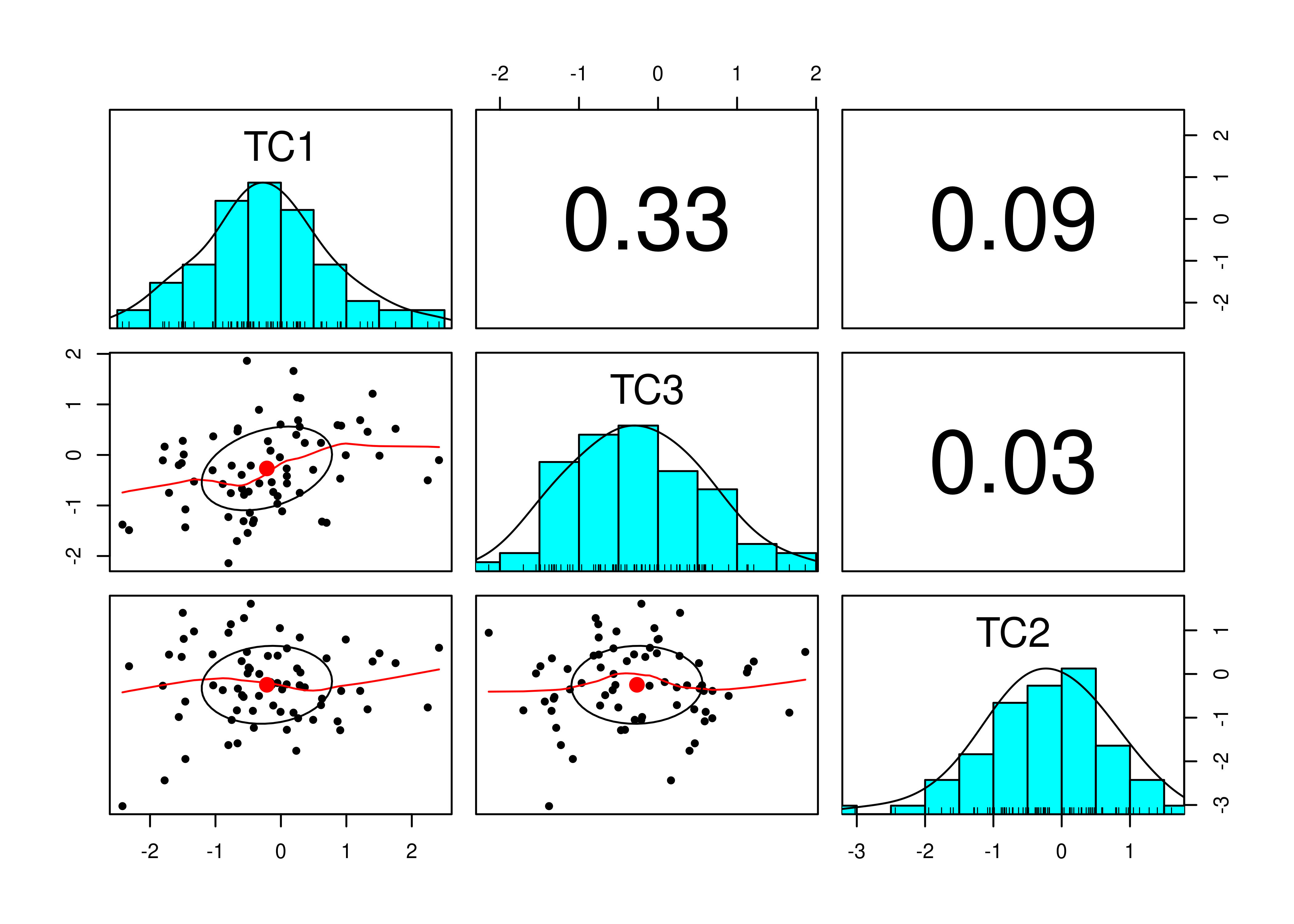

14.6 Benefits of Factor Analysis
Factor analysis has several benefits. First, factor analysis can be used for data reduction, similar to PCA. This is useful for reducing a large set of variables into a smaller set of factors that can be more easily analyzed. In addition, this data reduction can help to address multicollinearity issues in regression analyses. In addition to data reduction, factor analysis can help identify the structure of measures and constructs. Thus, factor analysis is particularly useful in the development, validation, and improvement of measures.
14.7 Conclusion
PCA is not factor analysis. PCA is a technique for data reduction, whereas factor analysis uses latent variables and can be used to identify the structure of measures/constructs or for data reduction. Many people use PCA when they should use factor analysis instead, such as when they are assessing latent constructs. Nevertheless, factor analysis has weaknesses including indeterminacy—i.e., a given data matrix can produce many different factor models, and you cannot determine which one is correct based on the data matrix alone. There are many decisions to make in factor analysis. These decisions can have important impacts on the resulting solution. Thus, it can be helpful for theory and interpretability to help guide decision-making when conducting factor analysis.
14.8 Suggested Readings
Floyd & Widaman (1995)
14.9 Exercises
14.9.1 Questions
Note: Several of the following questions use data from the Children of the National Longitudinal Survey of Youth Survey (CNLSY). The CNLSY is a publicly available longitudinal data set provided by the Bureau of Labor Statistics (https://www.bls.gov/nls/nlsy79-children.htm#topical-guide; archived at https://perma.cc/EH38-HDRN). The CNLSY data file for these exercises is located on the book’s page of the Open Science Framework (https://osf.io/3pwza). Children’s behavior problems were rated in 1988 (time 1: T1) and then again in 1990 (time 2: T2) on the Behavior Problems Index (BPI). Below are the items corresponding to the Antisocial subscale of the BPI:
- cheats or tells lies
- bullies or is cruel/mean to others
- does not seem to feel sorry after misbehaving
- breaks things deliberately
- is disobedient at school
- has trouble getting along with teachers
- has sudden changes in mood or feeling
- Fit an exploratory factor analysis (EFA) model using maximum likelihood to the seven items of the Antisocial subscale of the Behavior Problems Index at T1.
- Create a scree plot using the raw data (not the correlation or covariance matrix).
- How many factors should be retained according to the Kaiser–Guttman rule? How many factors should be retained according to a Parallel Test? Based on the available information, how many factors would you retain?
- Extract two factors with an oblique (oblimin) rotation. Which items load most strongly on Factor 1? Which items load most strongly on Factor 2? Why do you think these items load onto Factor 2? Which item has the highest cross-loading (on both Factors 1 and 2)?
- What is the association between Factors 1 and 2 when using an oblique rotation? What does this indicate about whether you should use an orthogonal or oblique rotation?
- For exercises about confirmatory factor analysis, see the exercises in Section #ref(semExercises) of the chapter on Structural Equation Modeling.
- Fit a principal component analysis (PCA) model to the seven items of the Antisocial subscale of the Behavior Problems Index at T1. How many components should be kept?
- Fit a one-factor confirmatory factor analysis (CFA) model to the seven items of the Antisocial subscale of the Behavior Problems Index at T1. Set the scale of the latent factor by standardizing the latent factor—set the mean of the factor to one and the variance of the factor to zero. Freely estimate the factor loadings of all indicators. Allow the residuals of indicators 5 and 6 to be correlated. Use full information maximum likelihood (FIML) to account for missing data. Use robust standard errors to account for non-normally distributed data.
- If your model fits well, why is it important to consider alternative models? What are some possible alternative models?
14.9.2 Answers
- A scree plot is in Figure 14.104.
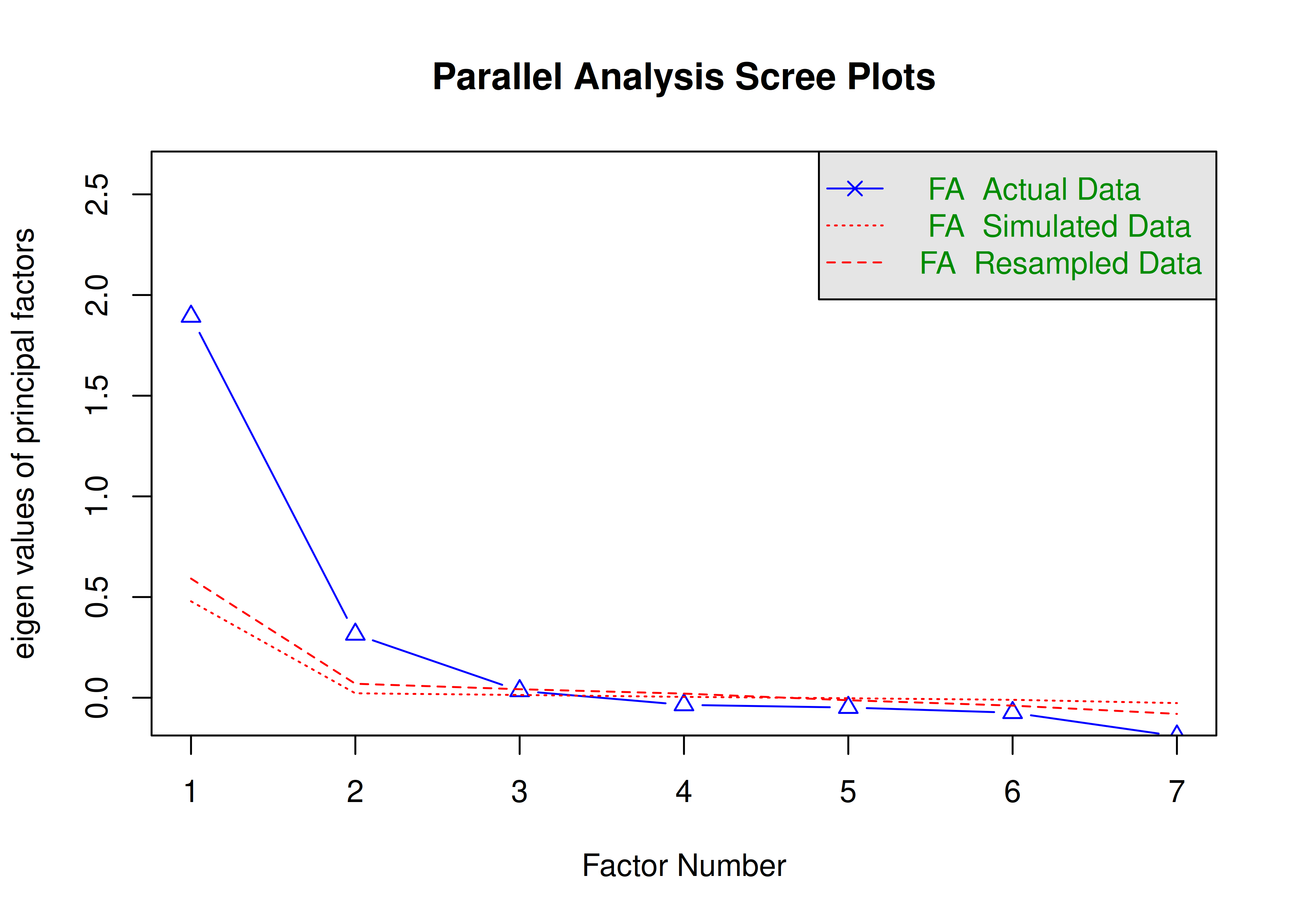
Figure 14.104: Scree Plot From Exploratory Factor Analysis.
- The Kaiser-Guttman rule states that all factors should be retained whose eigenvalues are greater than 1, because it is not conceptually elegant to include factors that explain less than one variable’s worth of variance (i.e., one eigenvalue). According to the Kaiser-Guttman rule, one factor should be retained in this case. However, for factor analysis (rather than PCA), we modify the guidelines to retain factors whose eigenvalues are greater than zero, so we would keep two factors. According to the Parallel Test, factors should be retained that explain more variance than randomly generated data. According to the Parallel Test, two factors should be retained.
- Items 1 (loading = .52), 2 (loading = .66), 3 (loading = .48), 4 (loading = .52), and 7 (loading = .39) load most strongly on Factor 1. Items 5 (“disobedient at school”; loading = 1.00) and 6 (“trouble getting along with teachers”; loading = .42) load most strongly on Factor 2. It is likely that these two items load onto a separate factor from the other antisocial items because they reflect school-related antisocial behavior. Item 6 has the highest cross-loading—in addition to loading onto Factor 2 (.42), it has a non-trivial loading on Factor 1 (.22).
- The association between Factors 1 and 2 is .48. This indicates that the factors are moderately correlated and that using an orthogonal rotation would likely be improper. An oblique rotation would be important to capture the association between the two factors. However, this could come at the expense of having simple structure and, therefore, straightforward interpretation of the factors.
- See the exercises on “Structural Equation Modeling” in Section 7.18.
- According to the Kaiser-Guttman rule and the Parallel Test, one component should be retained.
- The factor scores from the CFA model are correlated \(r = .97\) and \(r = .98\) with the factor scores of the EFA model and the component scores of the PCA model, respectively. The factor scores of the EFA model are correlated \(r = .997\) with the component scores of the PCA model.
- Even if a given model fits well, there are many other models that fit just as well. Any given data matrix can produce an infinite number of factor models that accurately represent the data structure (indeterminacy). For any model, there always exist an infinite number of models that fit exactly the same. There is no way to distinguish which factor model is correct from the data matrix. Although the fit of the structural model may be consistent with the hypothesized model, fit does not demonstrate that a given model is uniquely valid. Thus, it is important to consider alternative models that may better capture the causal processes, even if their fit is mathematically equivalent. For instance, you could consider models with multiple factors, correlated factors, correlated residuals, cross-loading indicators, regression paths, hierarchical (higher-order) factors, bifactors, etc. Remember, an important part of science is specifying and testing plausible alternative explanations! Some alternative, equivalently fitting models are in Figure 14.105.
Figure 14.105: Equivalently Fitting Models in Confirmatory Factor Analysis.