Overview of Factor Analysis
Factor analysis is a class of latent variable models that is designated to identify the structure of a measure or set of measures, and ideally, a construct or set of constructs. It aims to identify the optimal latent structure for a group of variables. Factor analysis encompasses two general types: confirmatory factor analysis and exploratory factor analysis. Exploratory factor analysis (EFA) is a latent variable modeling approach that is used when the researcher has no a priori hypotheses about how a set of variables is structured. EFA seeks to identify the empirically optimal-fitting model in ways that balance accuracy (i.e., variance accounted for) and parsimony (i.e., simplicity). Confirmatory factor analysis (CFA) is a latent variable modeling approach that is used when a researcher wants to evaluate how well a hypothesized model fits, and the model can be examined in comparison to alternative models. Using a CFA approach, the researcher can pit models representing two theoretical frameworks against each other to see which better accounts for the observed data.
Factor analysis is considered to be a “pure” data-driven method for identifying the structure of the data, but the “truth” that we get depends heavily on the decisions we make regarding the parameters of our factor analysis (Floyd & Widaman, 1995; Sarstedt et al., 2024). The goal of factor analysis is to identify simple, parsimonious factors that underlie the “junk” (i.e., scores filled with measurement error) that we observe.
It used to take a long time to calculate a factor analysis because it was computed by hand. Now, it is fast to compute factor analysis with computers (e.g., oftentimes less than 30 ms). In the 1920s, Spearman developed factor analysis to understand the factor structure of intelligence. It was a long process—it took Spearman around one year to calculate the first factor analysis! Factor analysis takes a large dimension data set and simplifies it into a smaller set of factors that are thought to reflect underlying constructs. If you believe that nature is simple underneath, factor analysis gives nature a chance to display the simplicity that lives beneath the complexity on the surface. Spearman identified a single factor, g, that accounted for most of the covariation between the measures of intelligence.
Factor analysis involves observed (manifest) variables and unobserved (latent) factors. In a reflective model, it is assumed that the latent factor influences the manifest variables, and the latent factor therefore reflects the common (reliable) variance among the variables. A factor model potentially includes factor loadings, residuals (errors or disturbances), intercepts/means, covariances, and regression paths. A regression path indicates a hypothesis that one variable (or factor) influences another. The standardized regression coefficient represents the strength of association between the variables or factors. A factor loading is a regression path from a latent factor to an observed (manifest) variable. The standardized factor loading represents the strength of association between the variable and the latent factor. A residual is variance in a variable (or factor) that is unexplained by other variables or factors. An indicator’s intercept is the expected value of the variable when the factor(s) (onto which it loads) is equal to zero. Covariances are the associations between variables (or factors). A covariance path between two variables represents omitted shared cause(s) of the variables. For instance, if you depict a covariance path between two variables, it means that there is a shared cause of the two variables that is omitted from the model (for instance, if the common cause is not known or was not assessed).
In factor analysis, the relation between an indicator (\(\text{X}\)) and its underlying latent factor(s) (\(\text{F}\)) can be represented with a regression formula as in Equation 14.1:
\[
\text{X} = \lambda \cdot \text{F} + \text{Item Intercept} + \text{Error Term}
\tag{14.1}\]
where:
-
\(\text{X}\) is the observed value of the indicator
-
\(\lambda\) is the factor loading, indicating the strength of the association between the indicator and the latent factor(s)
-
\(\text{F}\) is the person’s value on the latent factor(s)
-
\(\text{Item Intercept}\) represents the constant term that accounts for the expected value of the indicator when the latent factor(s) are zero
-
\(\text{Error Term}\) is the residual, indicating the extent of variance in the indicator that is not explained by the latent factor(s)
When the latent factors are uncorrelated, the (standardized) error term for an indicator is calculated as 1 minus the sum of squared standardized factor loadings for a given item (including cross-loadings).
Another class of factor analysis models are higher-order (or hierarchical) factor models and bifactor models. Guidelines in using higher-order factor and bifactor models are discussed by Markon (2019).
Factor analysis is a powerful technique to help identify the factor structure that underlies a measure or construct. As discussed in Section 14.1.4, however, there are many decisions to make in factor analysis, in addition to questions about which variables to use, how to scale the variables, etc. (Floyd & Widaman, 1995; Sarstedt et al., 2024). If the variables going into a factor analysis are not well assessed, factor analysis will not rescue the factor structure. In such situations, there is likely to be the problem of garbage in, garbage out. Factor analysis depends on the covariation among variables. Given the extensive method variance that measures have, factor analysis (and principal component analysis) tends to extract method factors. Method factors are factors that are related to the methods being assessed rather than the construct of interest. However, multitrait-multimethod approaches to factor analysis (such as in Section 14.4.2.13) help better partition the variance in variables that reflects method variance versus construct variance, to get more accurate estimates of constructs.
Floyd & Widaman (1995) provide an overview of factor analysis for the development of clinical assessments.
Example Factor Models from Correlation Matrices
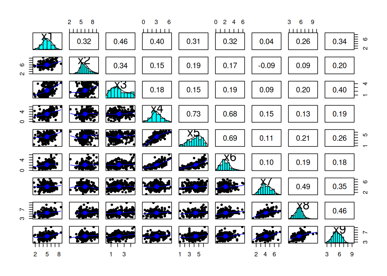
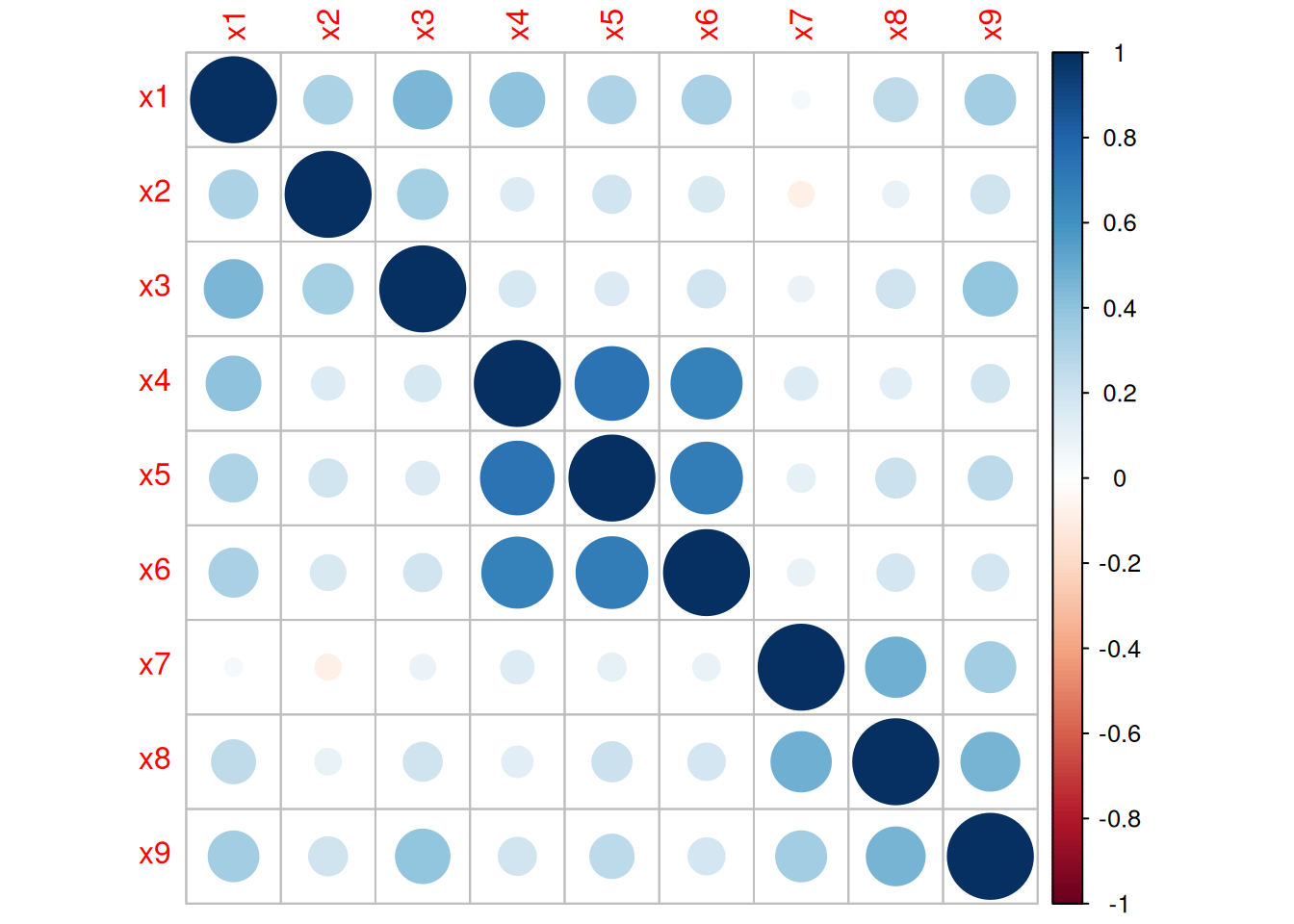
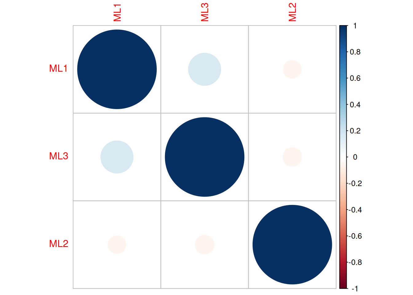
Before pursuing factor analysis, it is helpful to evaluate the extent to which the variables are intercorrelated. If the variables are not correlated (or are correlated only weakly), there is no reason to believe that a common factor influences them, and thus factor analysis would not be useful. So, before conducting a factor analysis, it is important to examine the correlation matrix of the variables to determine whether the variables intercorrelate strongly enough to justify a factor analysis.
Below, I provide some example factor models from various correlation matrices. Analytical examples of factor analysis are presented in Section 14.4.
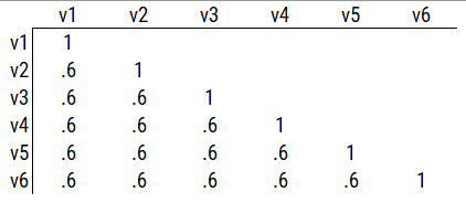
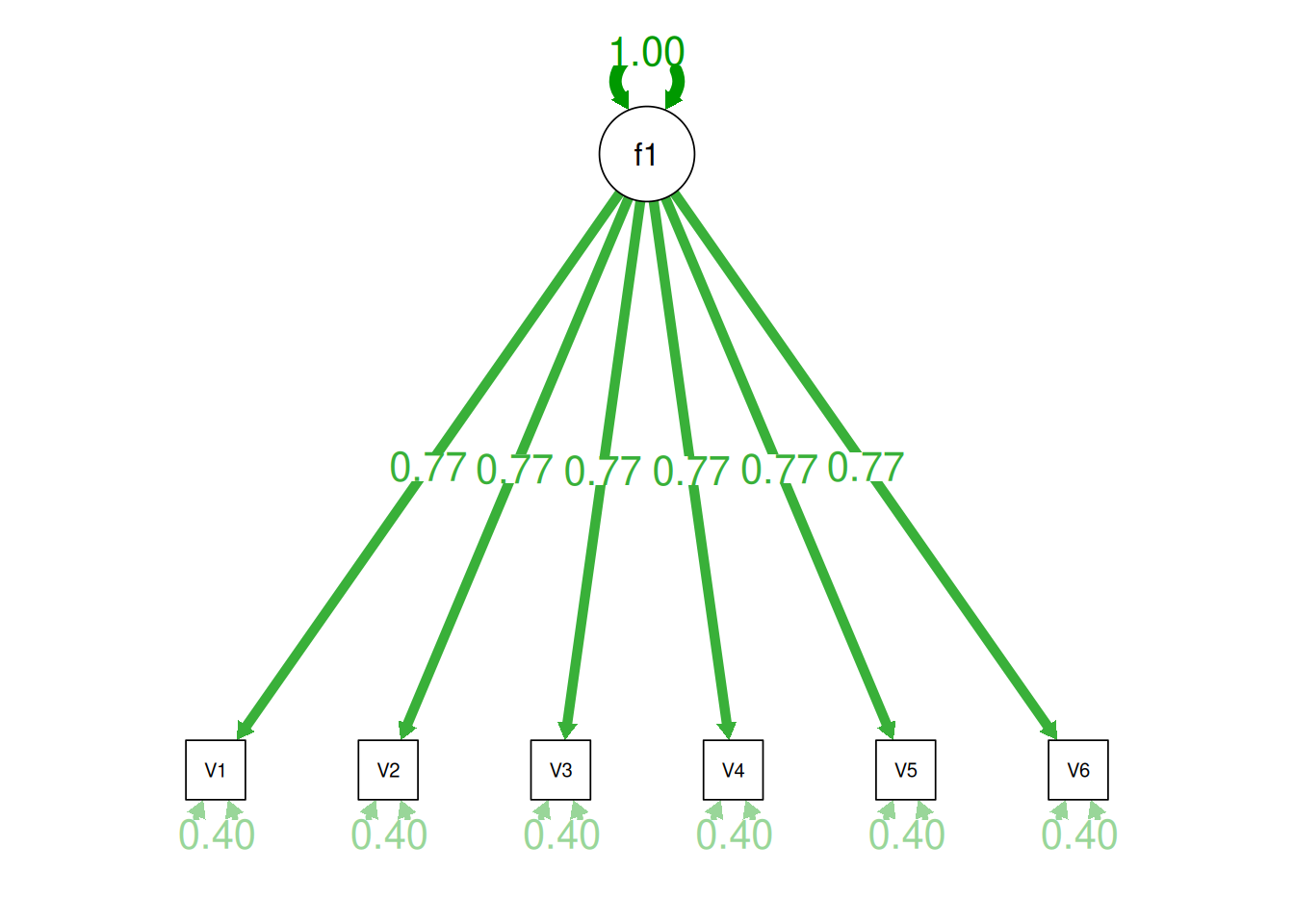
Consider the example correlation matrix in Figure 14.1. Because all of the correlations are the same (\(r = .60\)), we expect there is approximately one factor for this pattern of data.
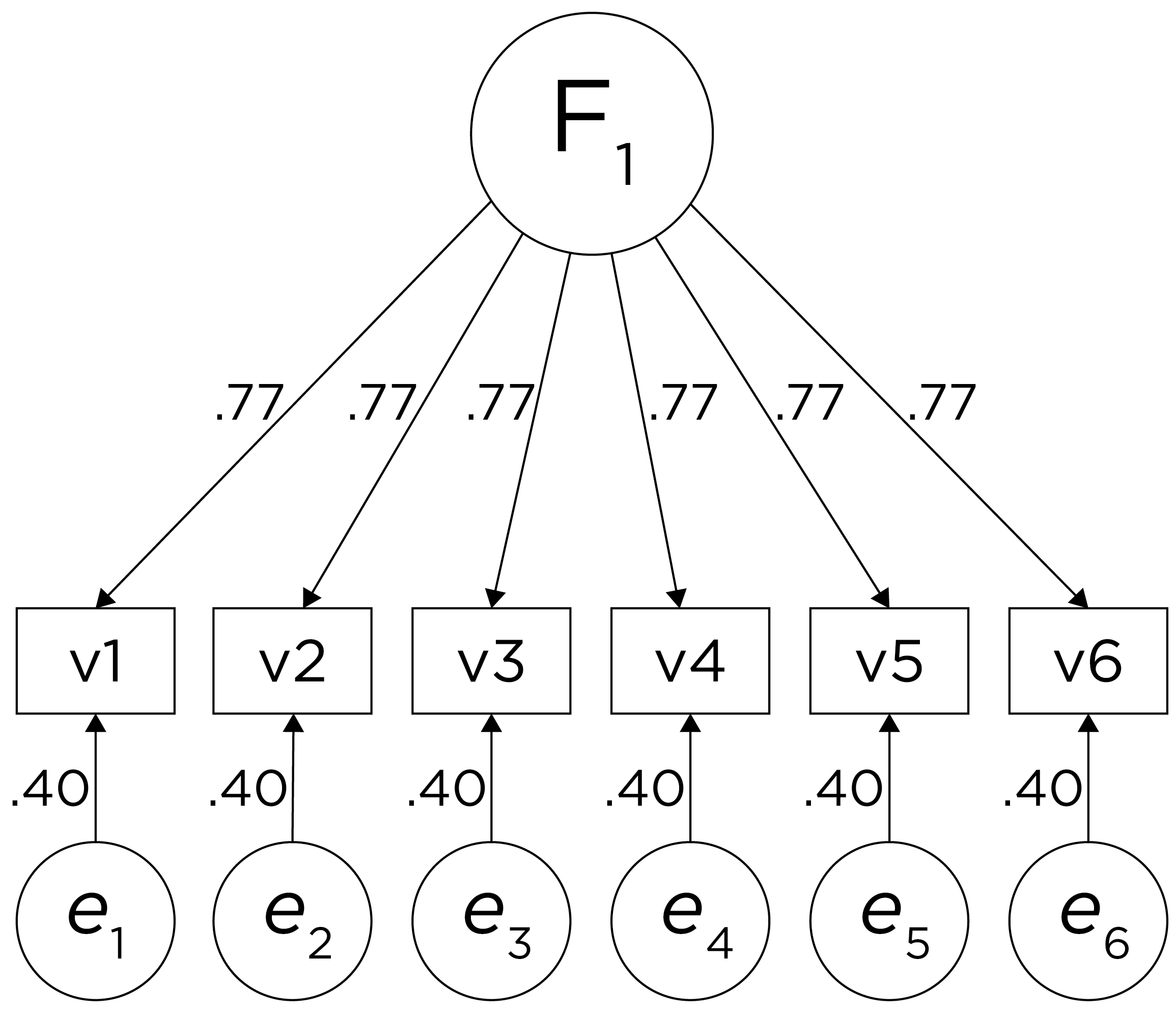
In a single-factor model fit to these data, the factor loadings are .77 and the residual error terms are .40, as depicted in Figure 14.2. The amount of common variance (\(R^2\)) that is accounted for by an indicator is estimated as the square of the standardized loading: \(.60 = .77 \times .77\). The amount of error for an indicator is estimated as: \(\text{error} = 1 - \text{common variance}\), so in this case, the amount of error is: \(.40 = 1 - .60\). The proportion of the total variance in indicators that is accounted for by the latent factor is the sum of the square of the standardized loadings divided by the number of indicators. That is, to calculate the proportion of the total variance in the variables that is accounted for by the latent factor, you would square the loadings, sum them up, and divide by the number of variables: \(\frac{.77^2 + .77^2 + .77^2 + .77^2 + .77^2 + .77^2}{6} = \frac{.60 + .60 + .60 + .60 + .60 + .60}{6} = .60\). Thus, the latent factor accounts for 60% of the variance in the indicators. In this model, the latent factor explains the covariance among the variables. If the answer is simple, a small and parsimonious model should be able to obtain the answer.
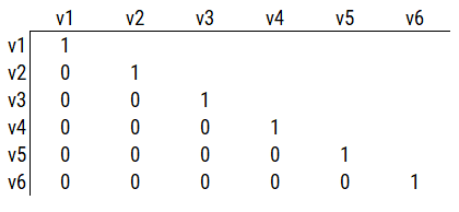
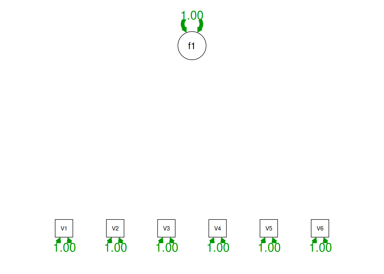
Consider a different correlation matrix in Figure 14.3. There is no common variance (correlations between the variables are zero), so there is no reason to believe there is a common factor that influences all of the variables. Variables that are not correlated cannot be related by a third variable, such as a common factor, so a common factor is not the right model.
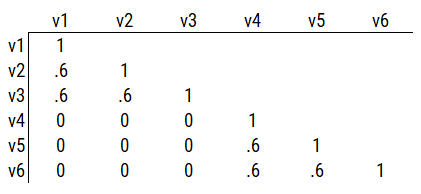
Consider another correlation matrix in Figure 14.4.
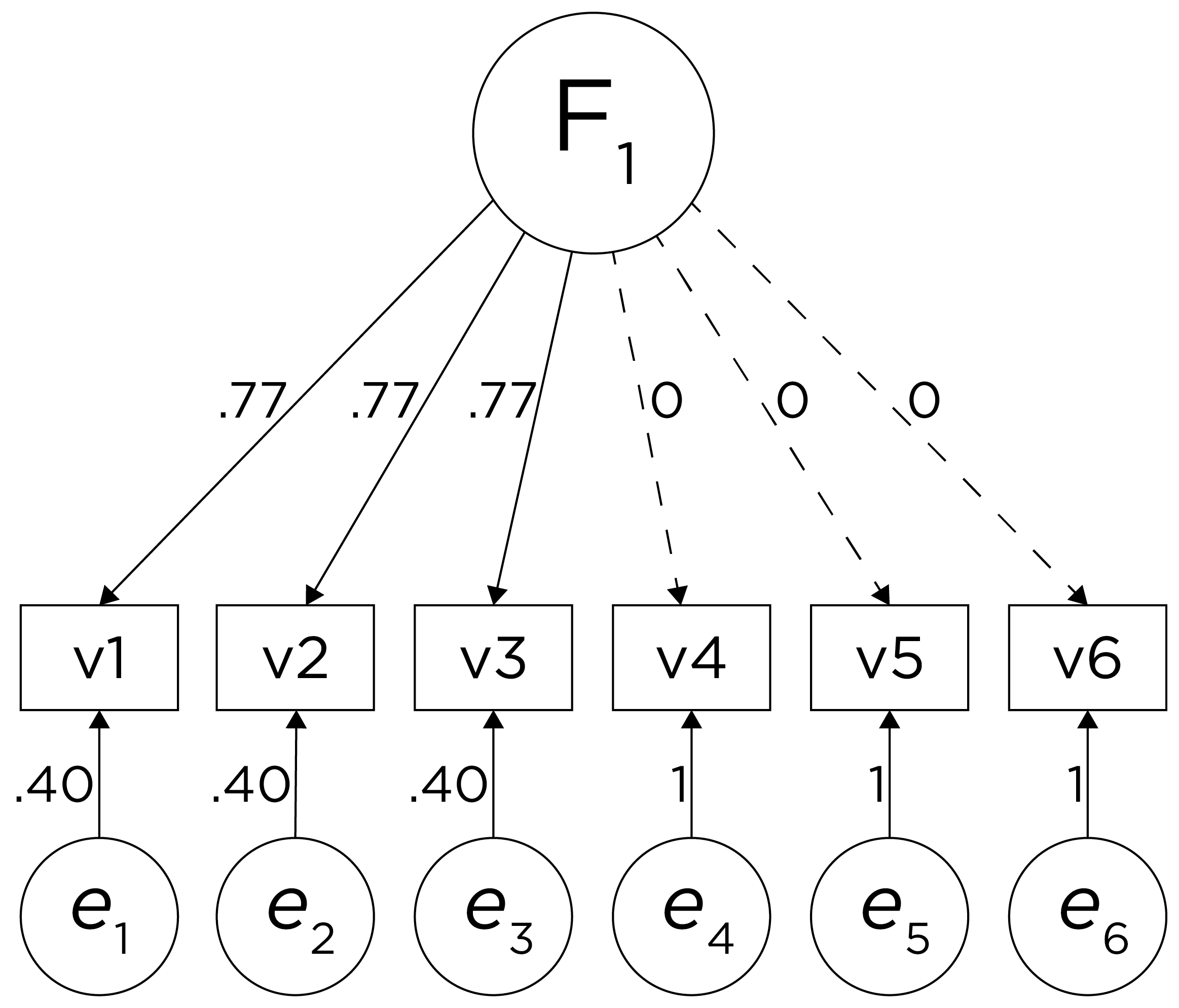
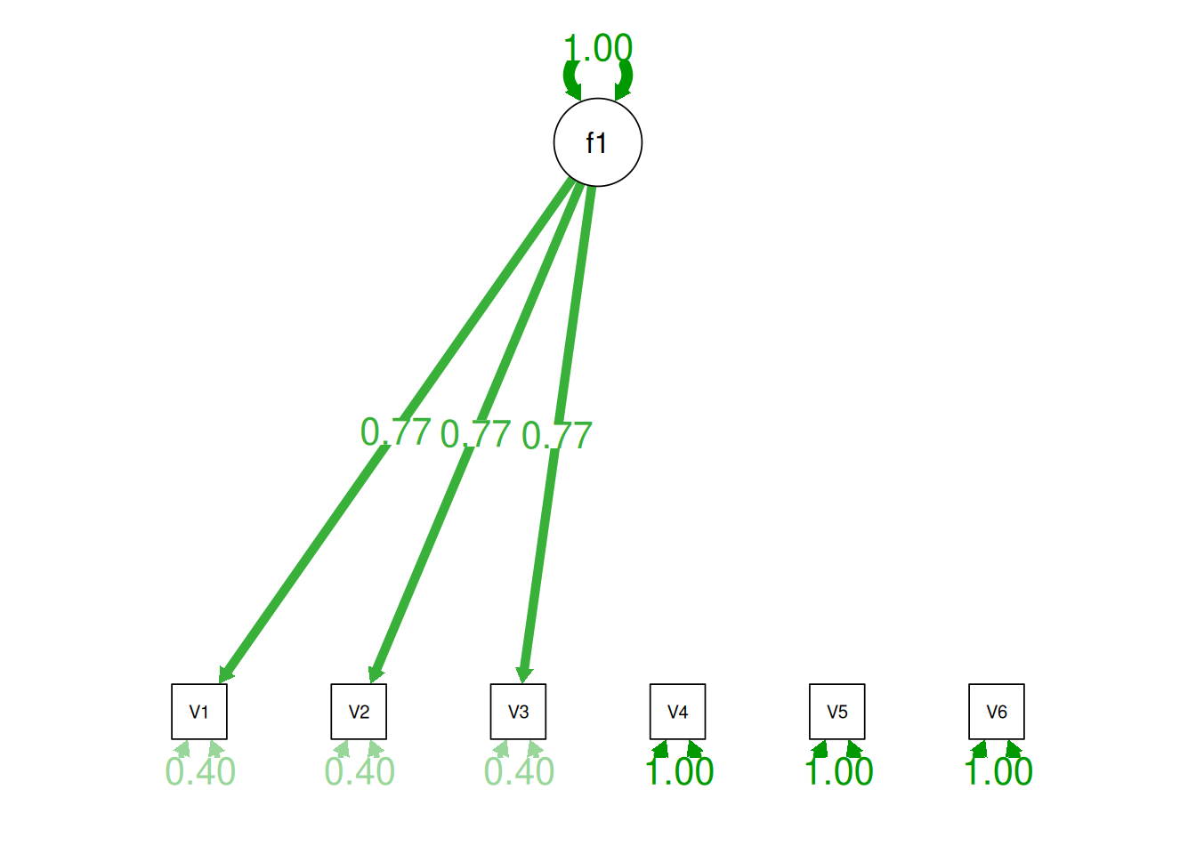
If you try to fit a single factor to this correlation matrix, it generates a factor model depicted in Figure 14.5. In this model, the first three variables have a factor loading of .77, but the remaining three variables have a factor loading of zero. This indicates that three remaining factors likely do not share a common factor with the first three variables.
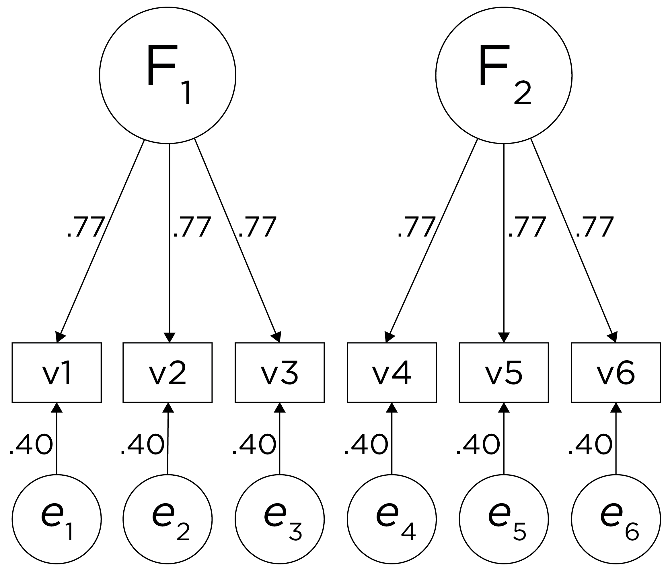
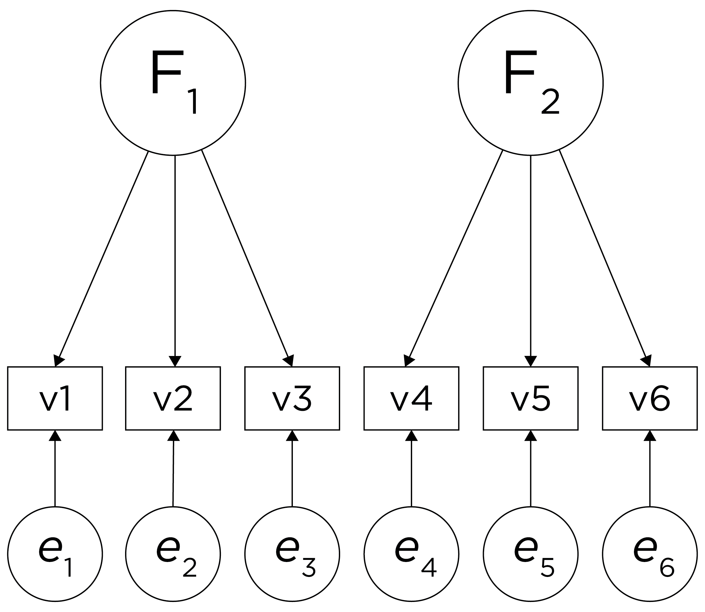
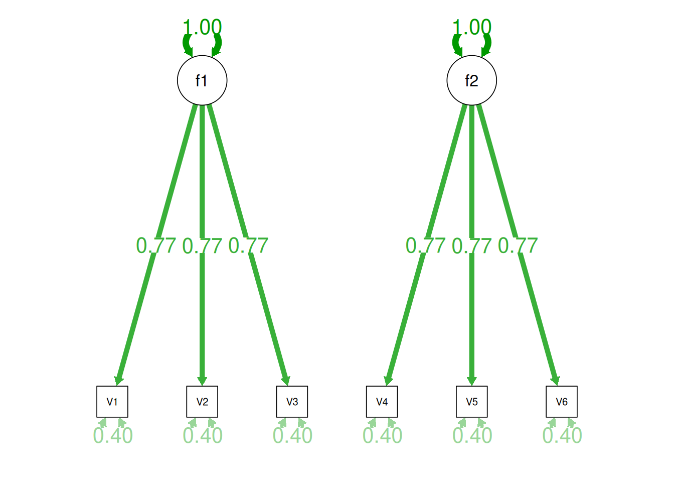
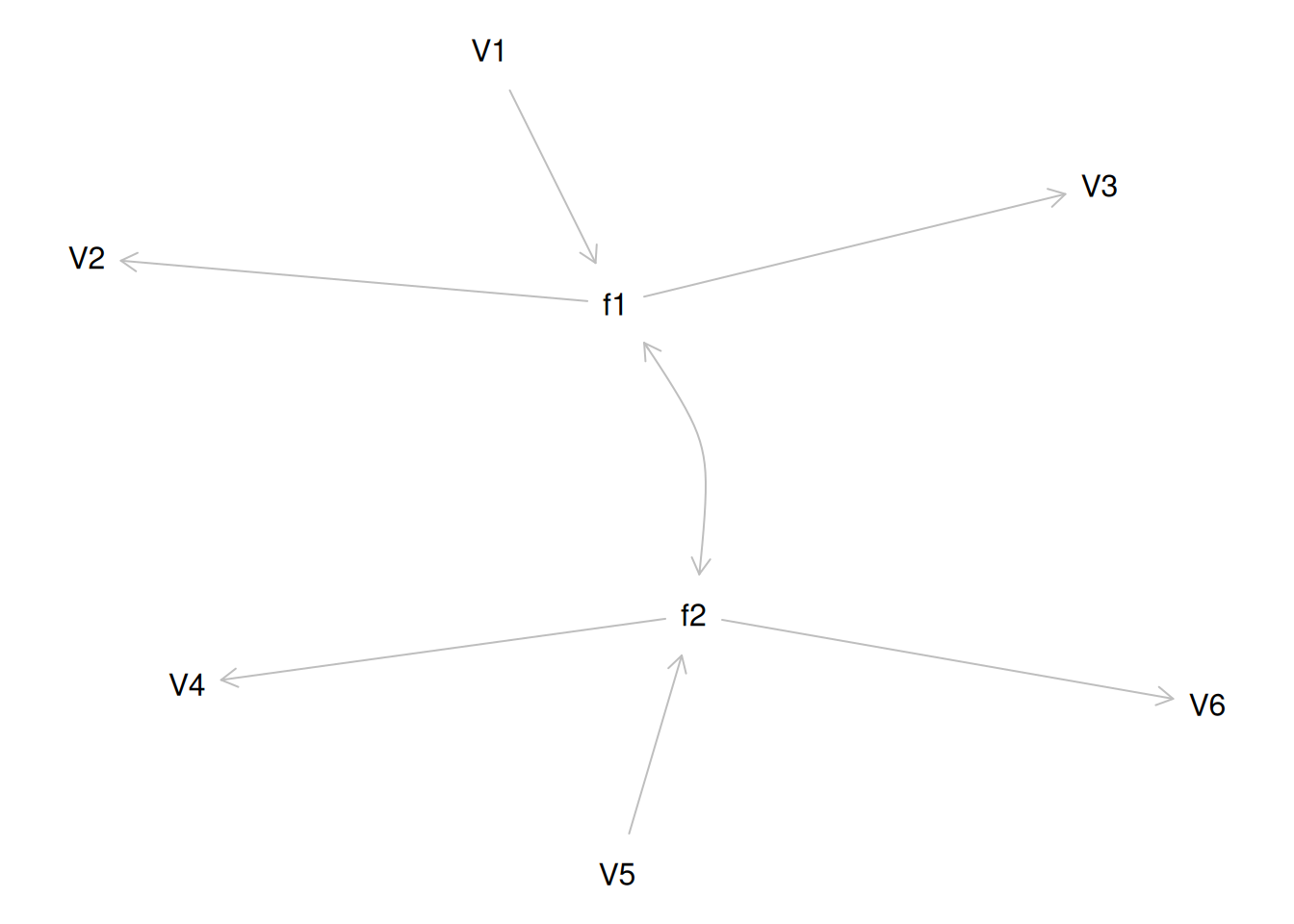
Therefore, a one-factor model is probably not correct; instead, the structure of the data is probably best represented by a two-factor model, as depicted in Figure 14.6. In the model, Factor 1 explains why measures 1, 2, and 3 are correlated, whereas Factor 2 explains why measures 4, 5, and 6 are correlated. A two-factor model thus explains why measures 1, 2, and 3 are not correlated with measures 4, 5, and 6. In this model, each latent factor accounts for 60% of the variance in the indicators that load onto it: \(\frac{.77^2 + .77^2 + .77^2}{3} = \frac{.60 + .60 + .60}{3} = .60\). Each latent factor accounts for 30% of the variance in all of the indicators: \(\frac{.77^2 + .77^2 + .77^2 + 0^2 + 0^2 + 0^2}{6} = \frac{.60 + .60 + .60 + 0 + 0 + 0}{6} = .30\).
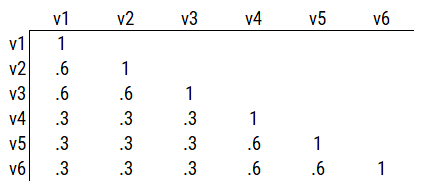
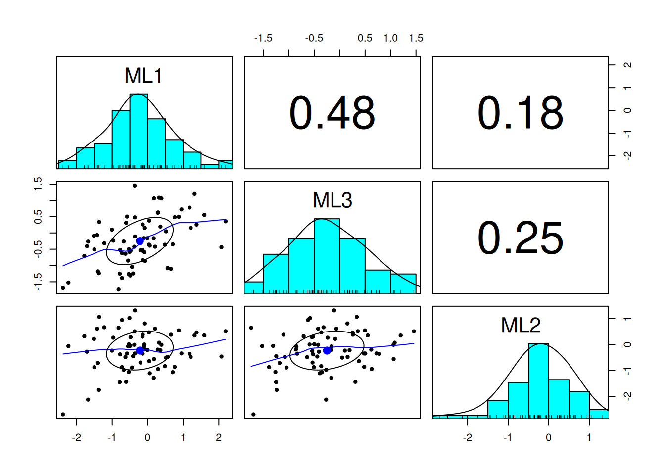
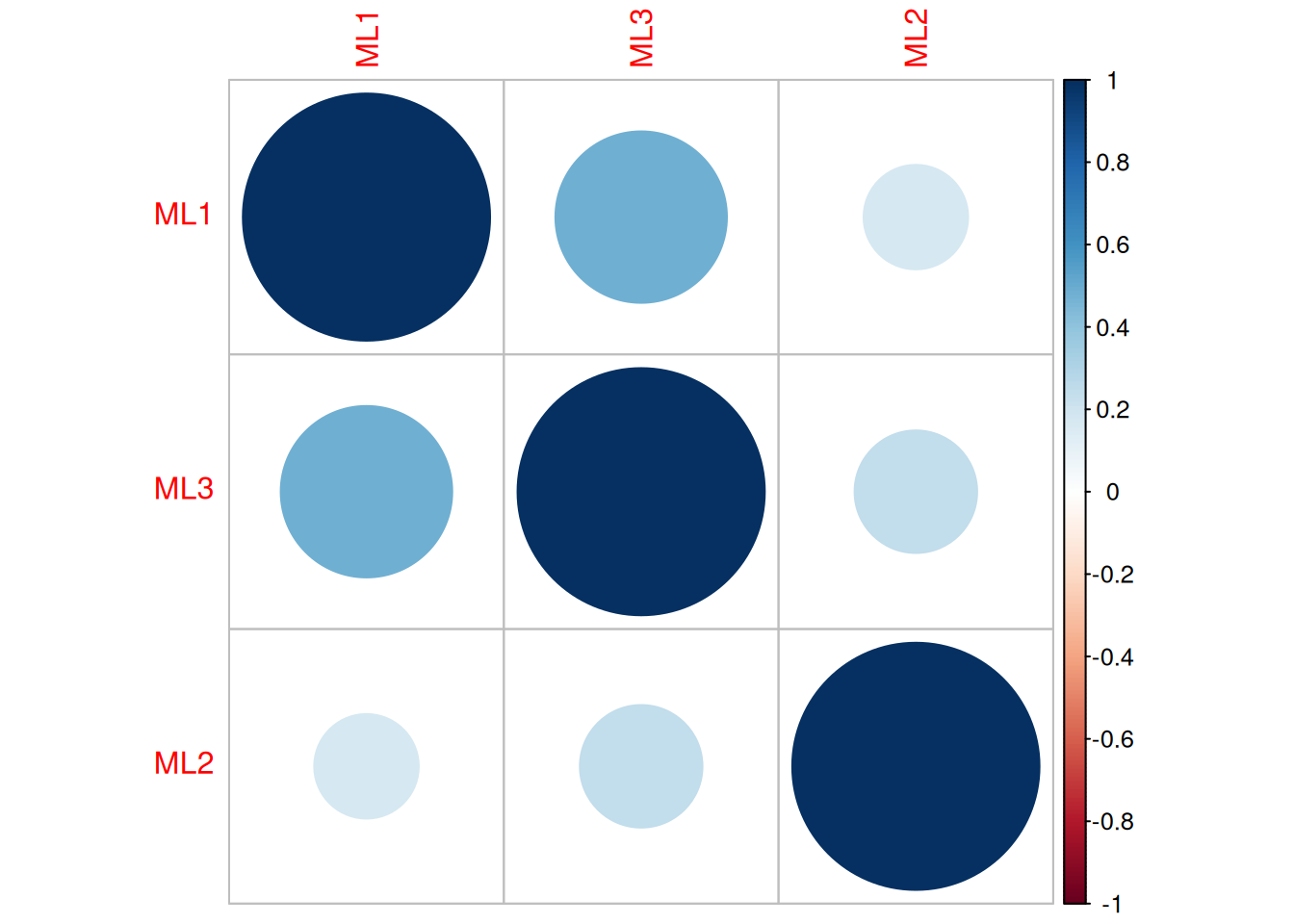
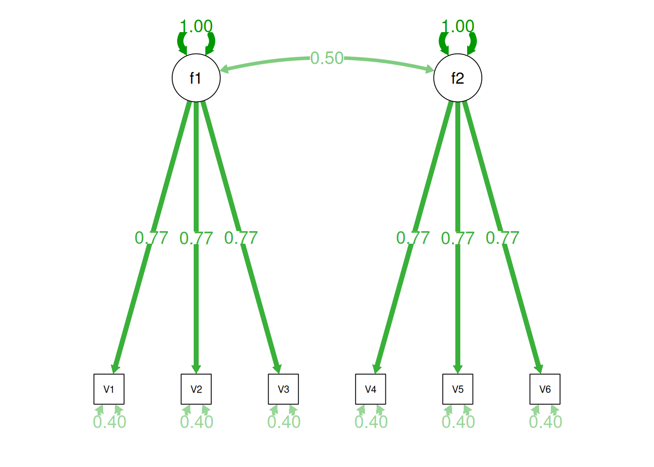
Consider another correlation matrix in Figure 14.7.
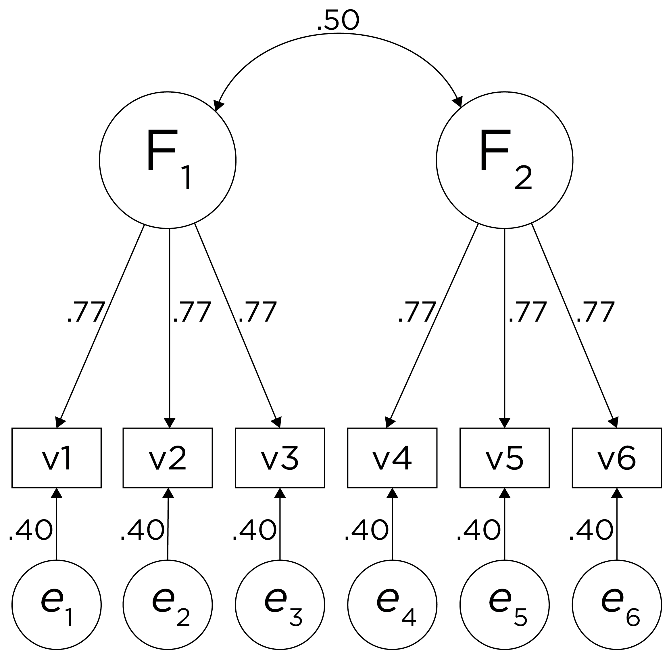
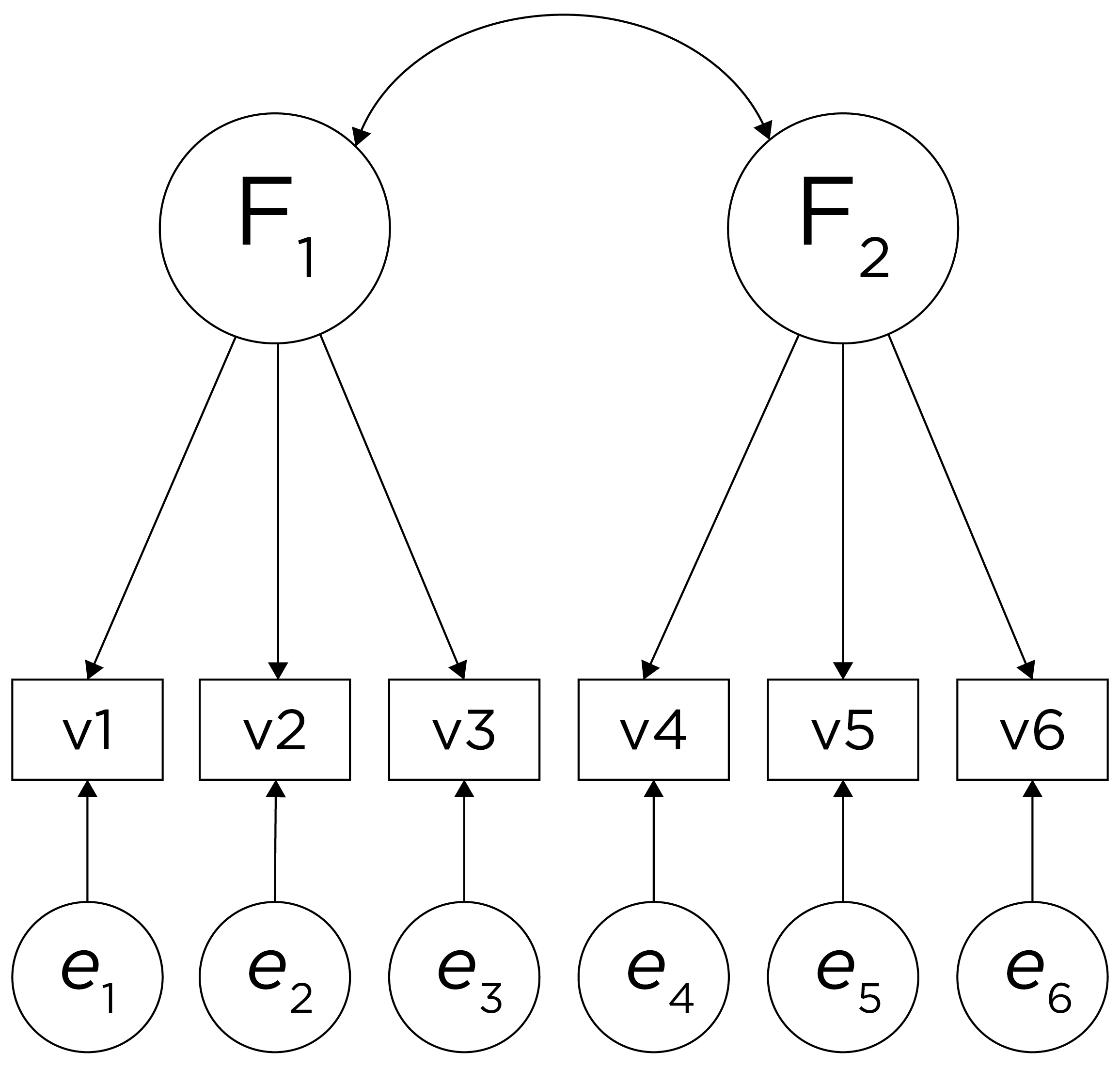
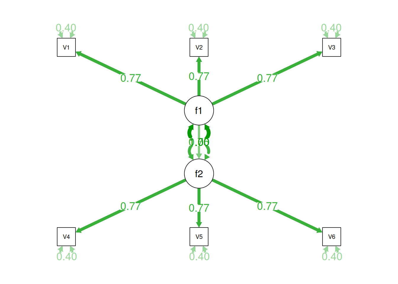
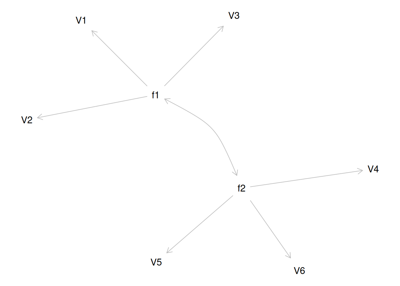
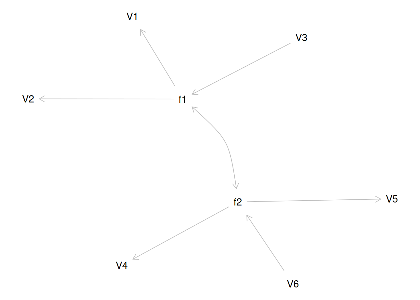
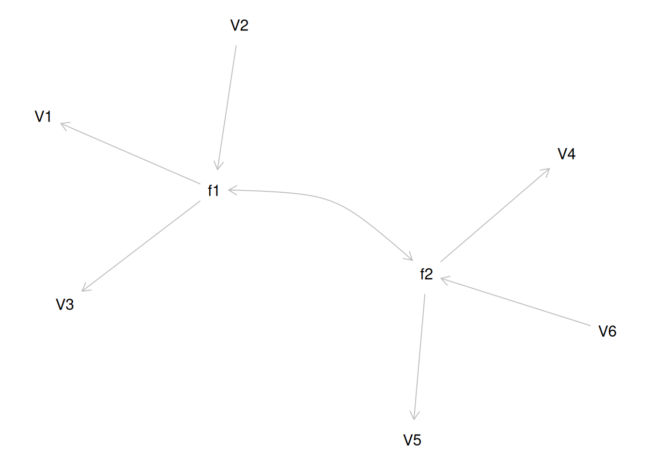
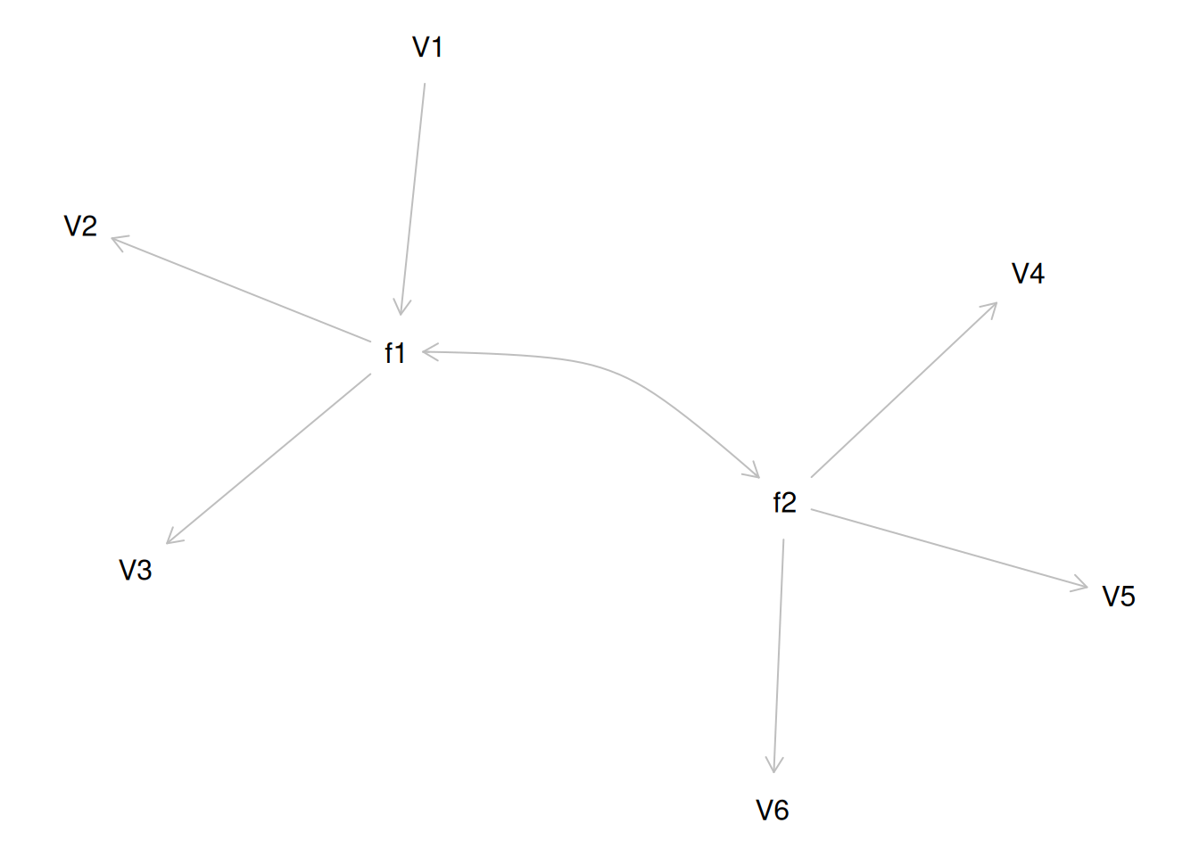
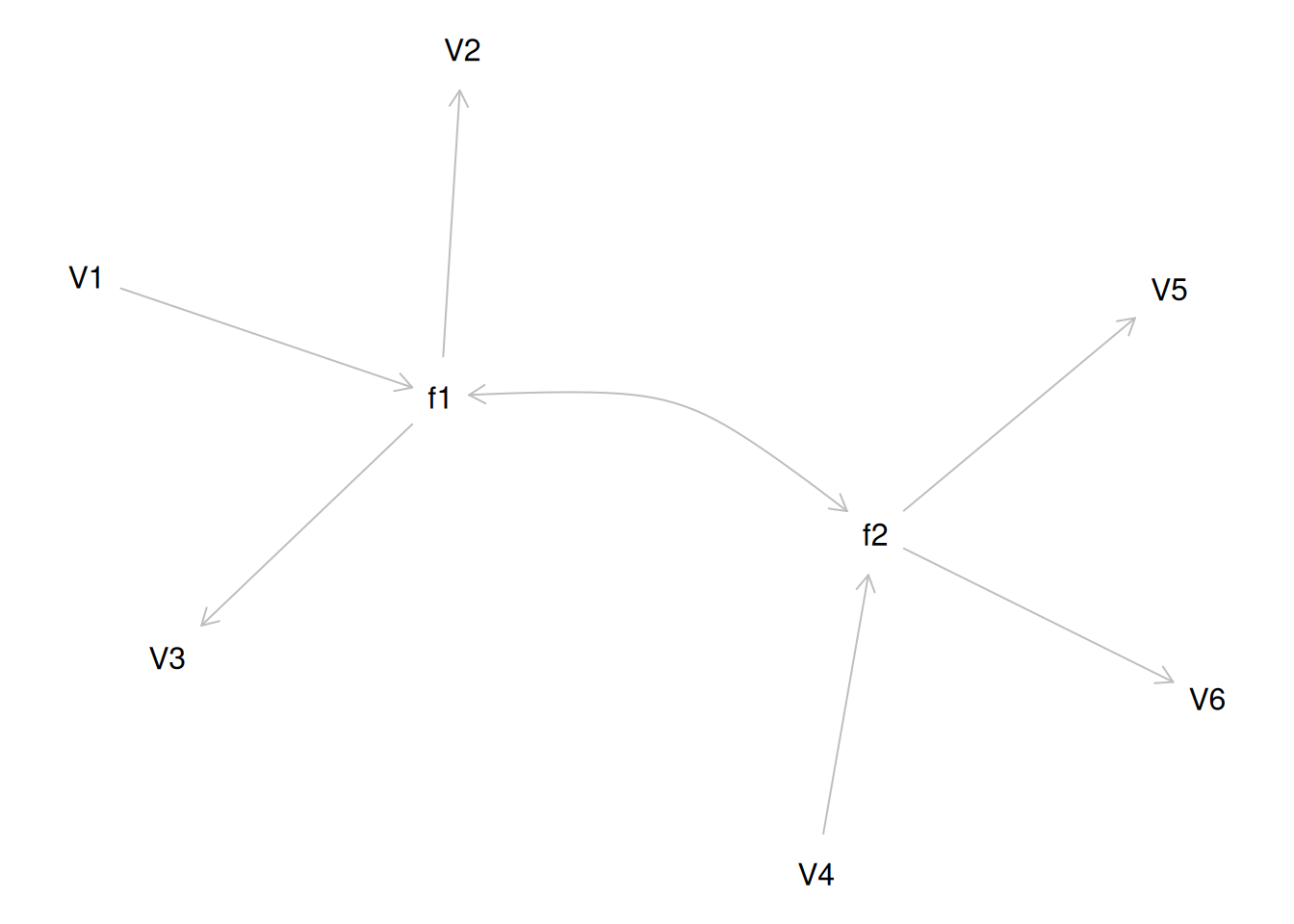
One way to model these data is depicted in Figure 14.8. In this model, the factor loadings are .77, the residual error terms are .40, and there is a covariance path of .50 for the association between Factor 1 and Factor 2. Going from the model to the correlation matrix is deterministic. If you know the model, you can calculate the correlation matrix. For instance, using path tracing rules (described in Section 4.1), the correlation of measures within a factor in this model is calculated as: \(0.60 = .77 \times .77\). Using path tracing rules, the correlation of measures across factors in this model is calculated as: \(.30 = .77 \times .50 \times .77\). In this model, each latent factor accounts for 60% of the variance in the indicators that load onto it: \(\frac{.77^2 + .77^2 + .77^2}{3} = \frac{.60 + .60 + .60}{3} = .60\). Each latent factor accounts for 37% of the variance in all of the indicators: \(\frac{.77^2 + .77^2 + .77^2 + (.50^2 \times .77^2) + (.50^2 \times .77^2) + (.50^2 \times .77^2)}{6} = \frac{.60 + .60 + .60 + .15 + .15 + .15}{6} = .37\).
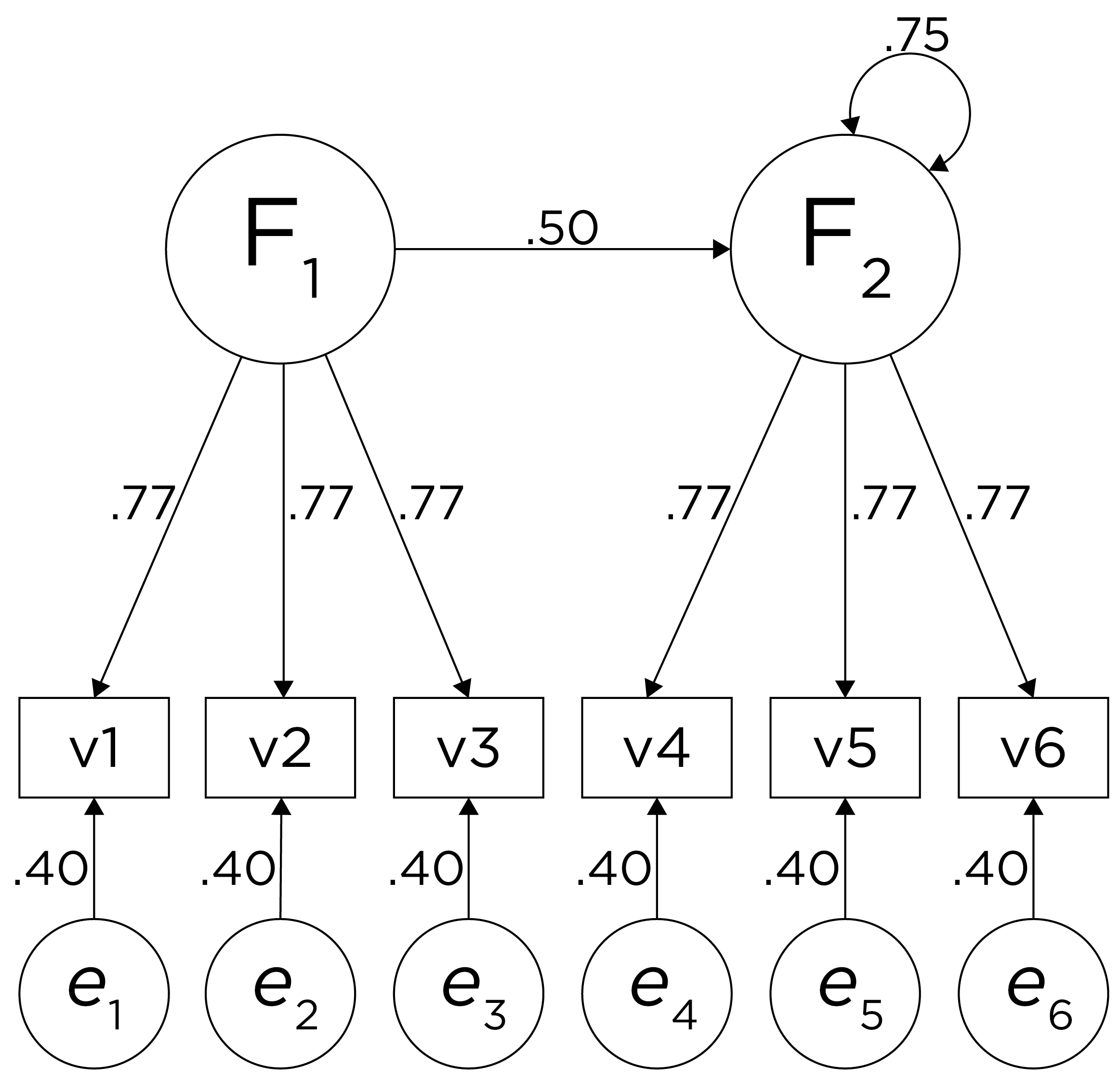
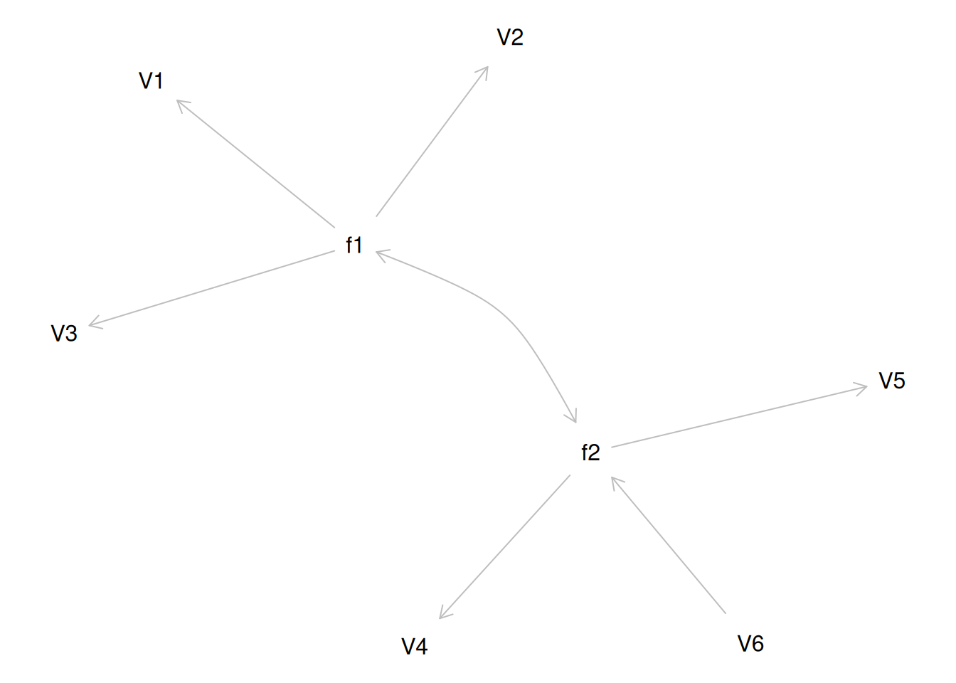
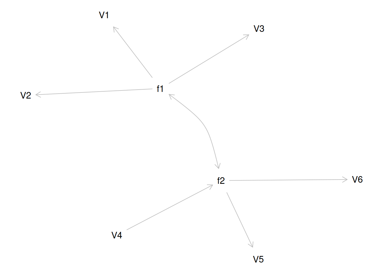
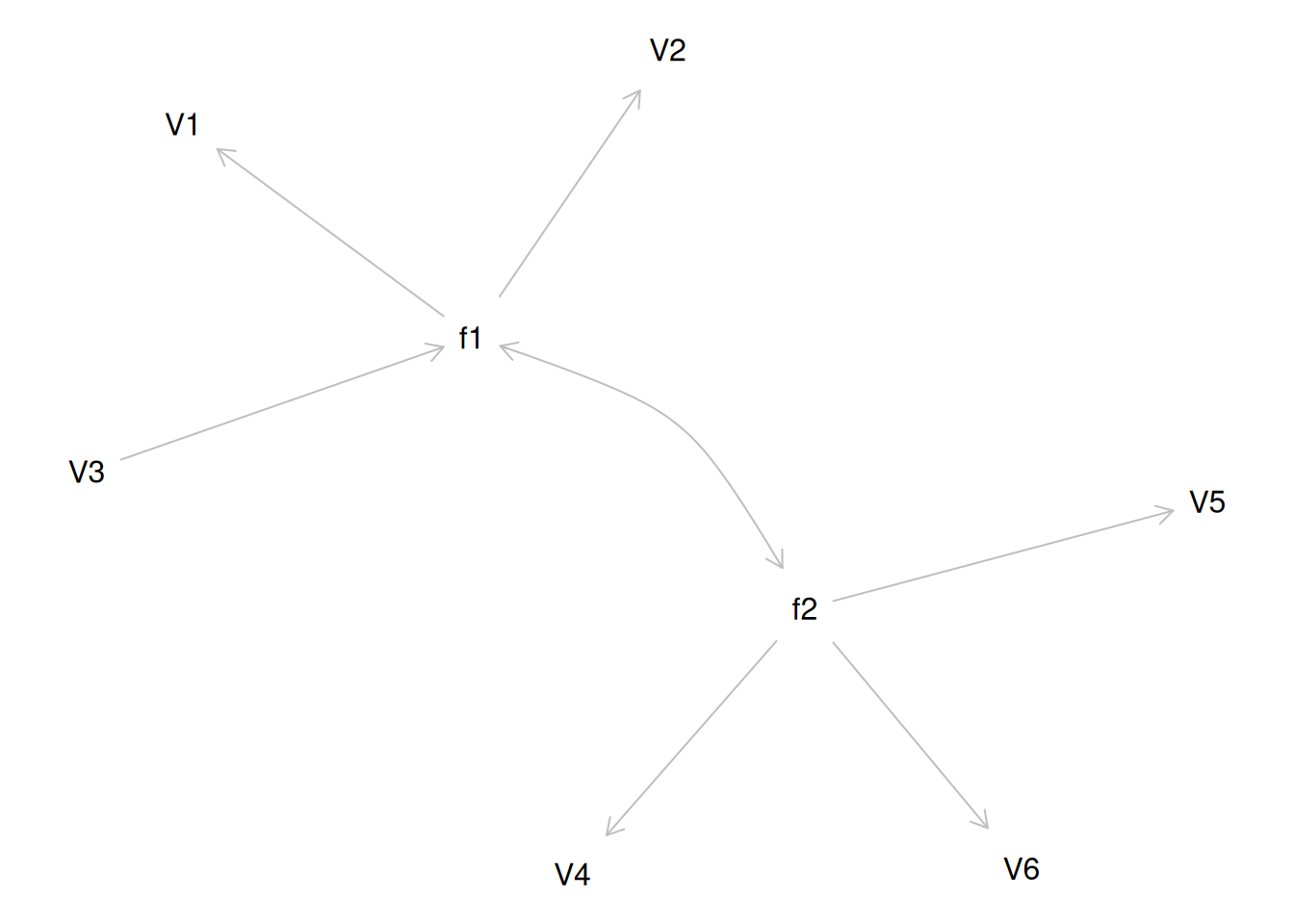
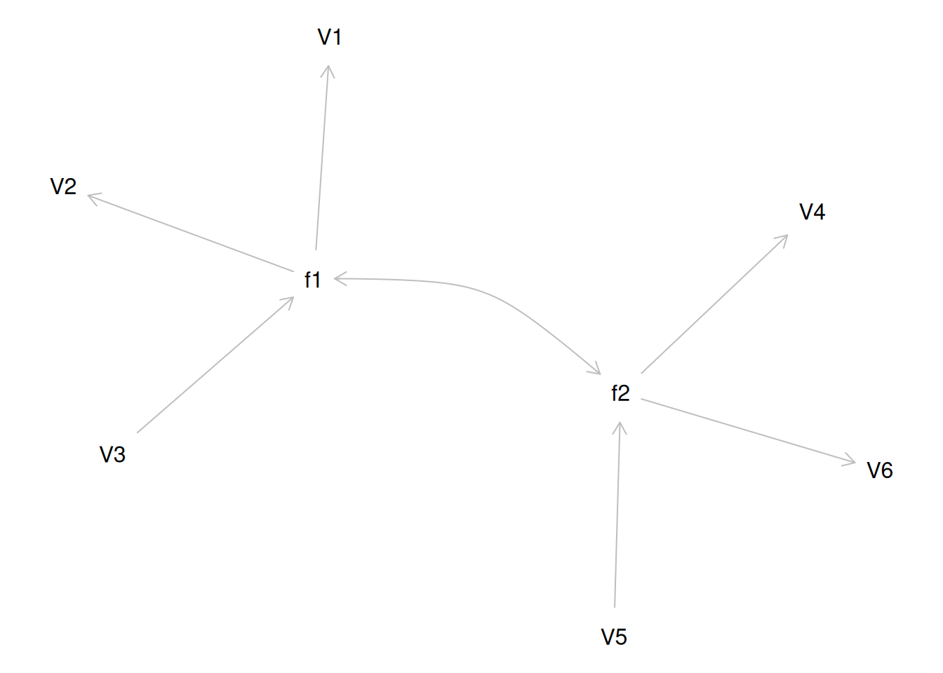
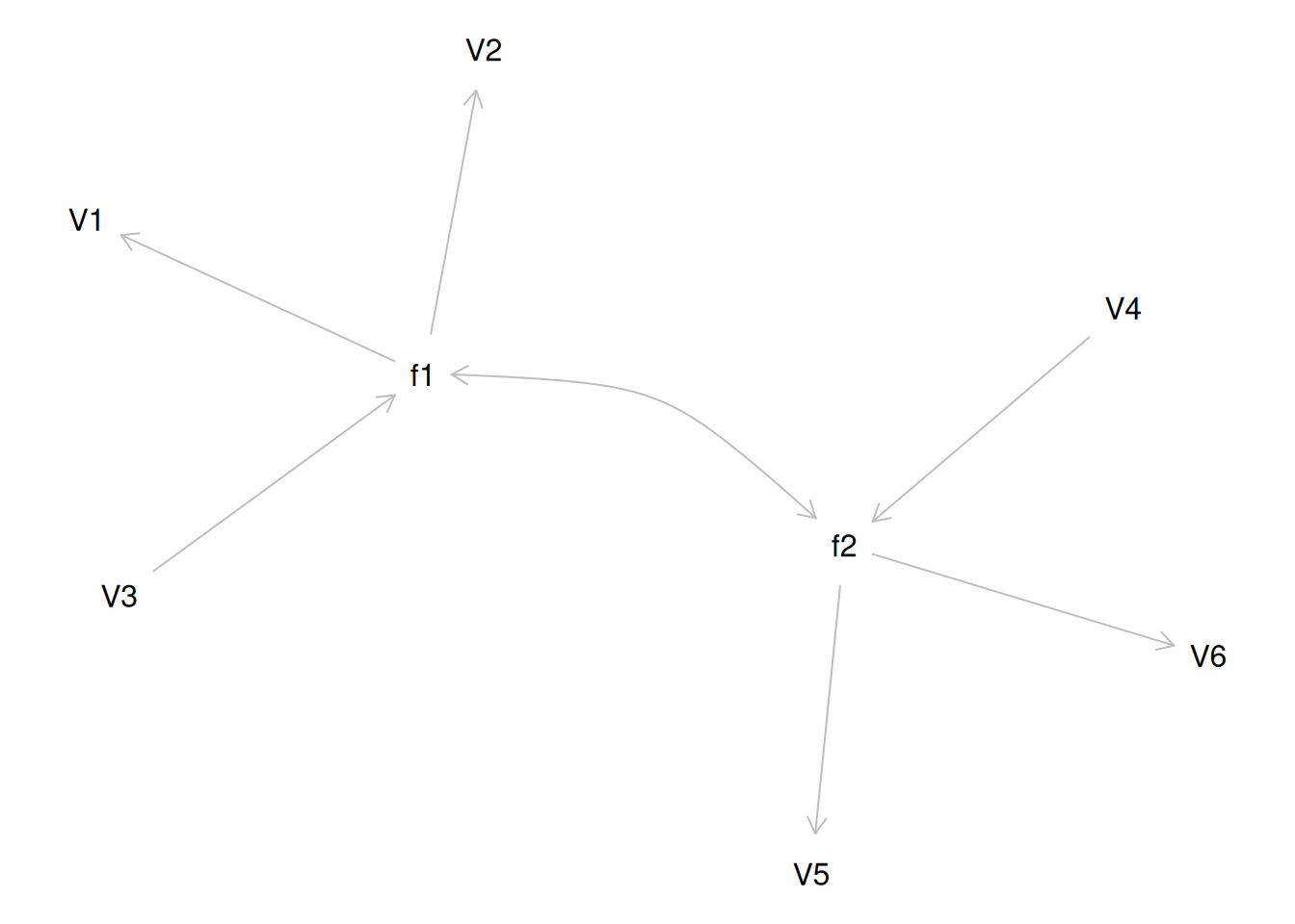
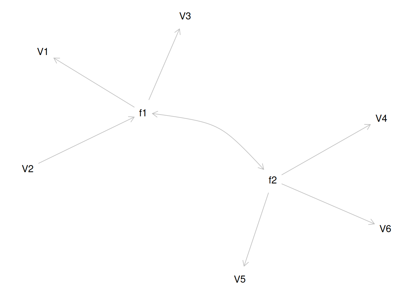
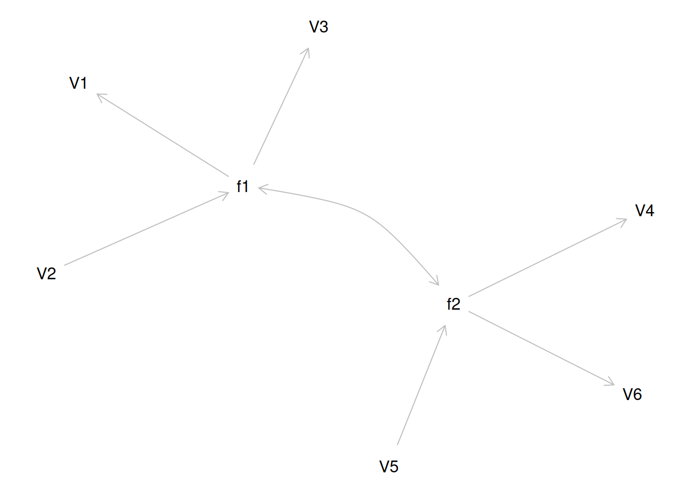
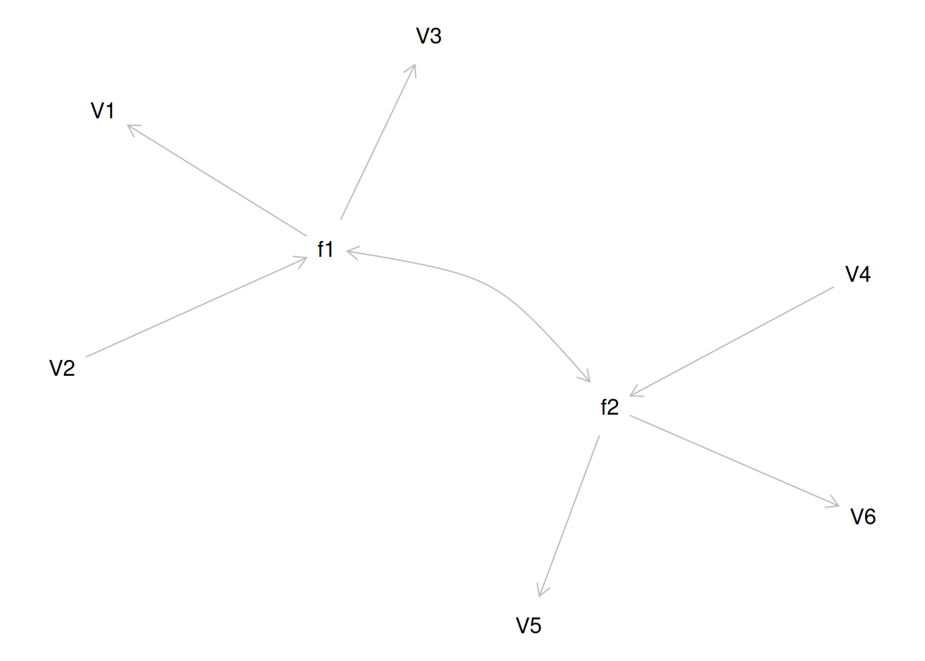
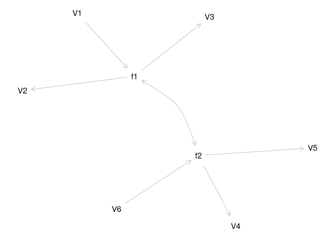
Although going from the model to the correlation matrix is deterministic, going from the correlation matrix to the model is not deterministic. If you know the correlation matrix, there may be many possible models. For instance, the model could also be the one depicted in Figure 14.9, with factor loadings of .77, residual error terms of .40, a regression path of .50, and a disturbance term of .75. The proportion of variance in Factor 2 that is explained by Factor 1 is calculated as: \(.25 = .50 \times .50\). The disturbance term is calculated as \(.75 = 1 - (.50 \times .50) = 1 - .25\). In this model, each latent factor accounts for 60% of the variance in the indicators that load onto it: \(\frac{.77^2 + .77^2 + .77^2}{3} = \frac{.60 + .60 + .60}{3} = .60\). Factor 1 accounts for 15% of the variance in the indicators that load onto Factor 2: \(\frac{(.50^2 \times .77^2) + (.50^2 \times .77^2) + (.50^2 \times .77^2)}{3} = \frac{.15 + .15 + .15}{3} = .15\). This model has the exact same fit as the previous model, but it has different implications. Unlike the previous model, in this model, there is a “causal” pathway from Factor 1 to Factor 2. However, the causal effect of Factor 1 does not account for all of the variance in Factor 2 because the correlation is only .50.
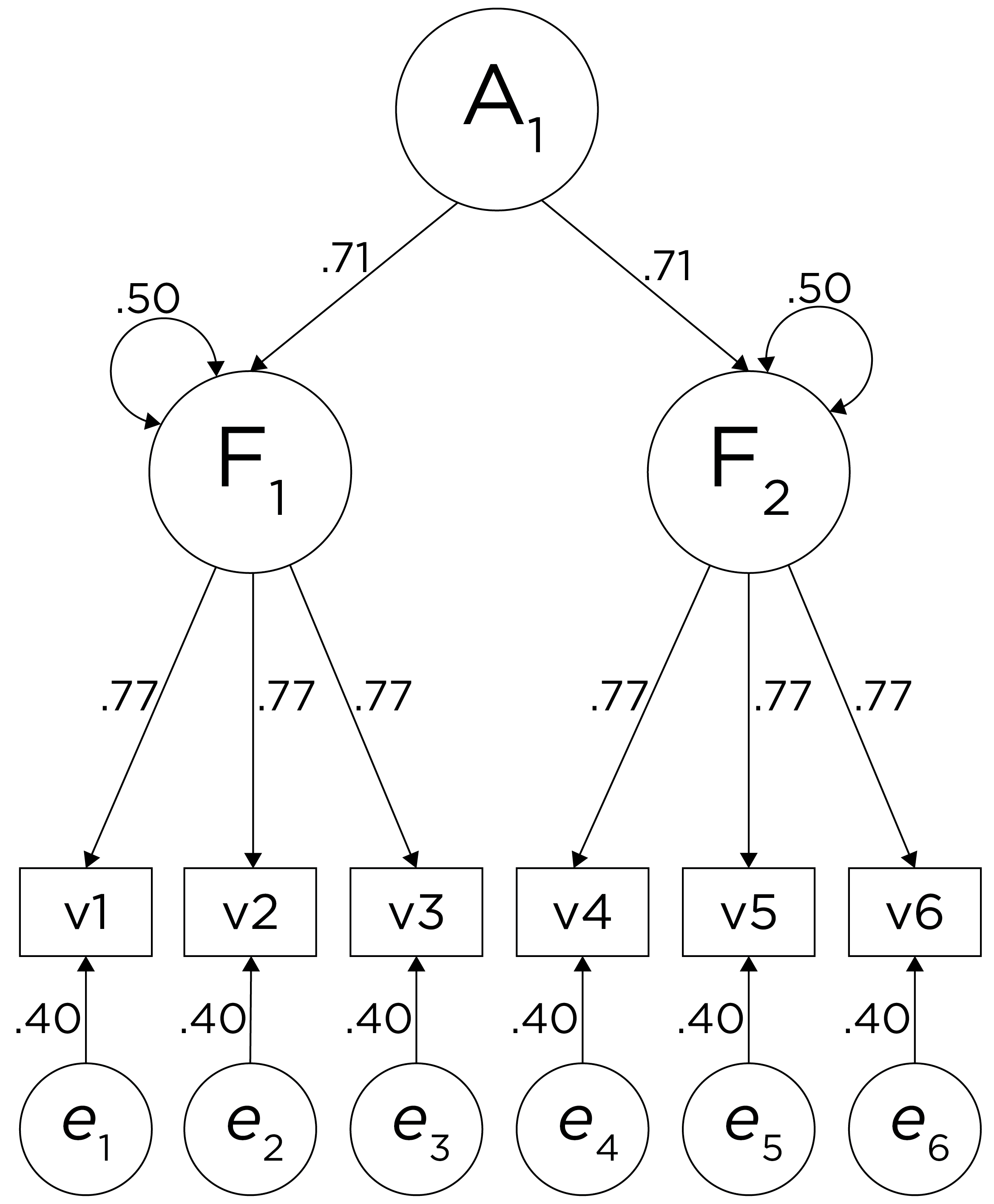
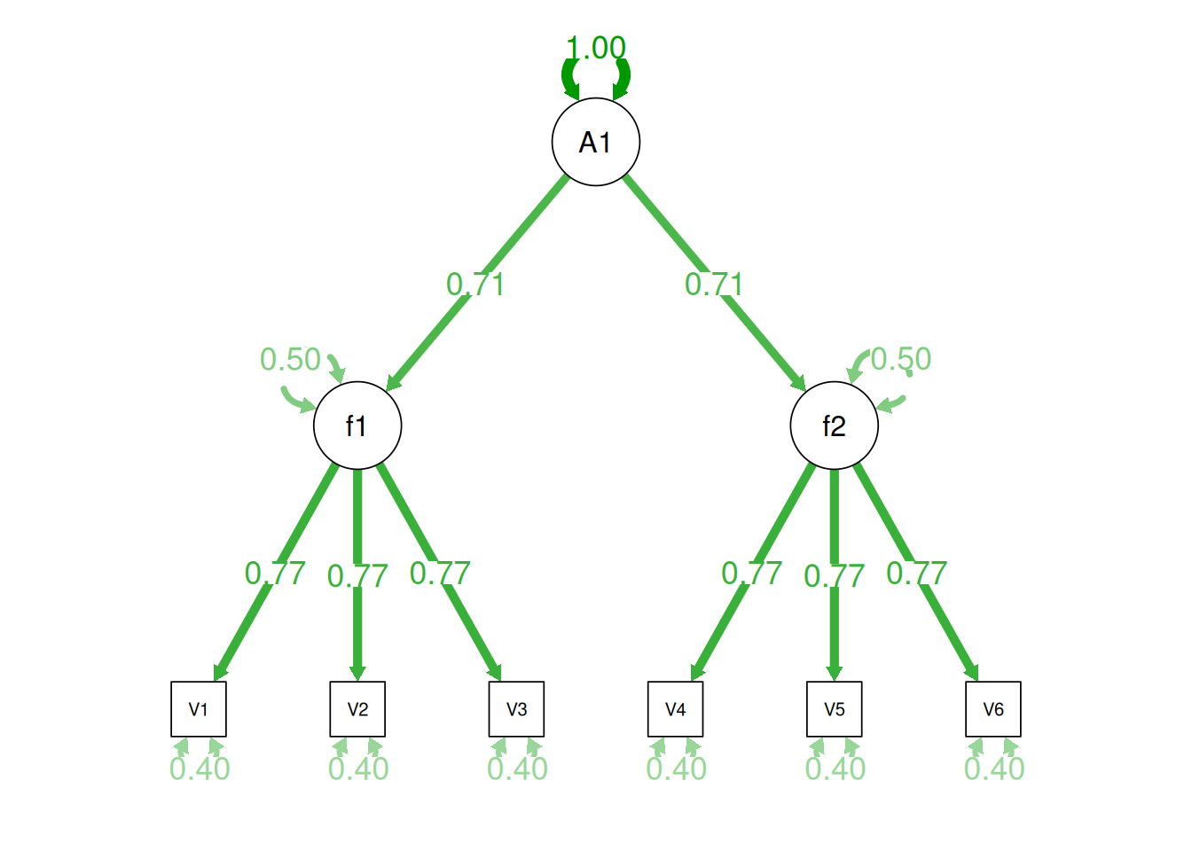
Alternatively, something else (e.g., another factor) could be explaining the data that we have not considered, as depicted in Figure 14.10. This is a higher-order factor model, in which there is a higher-order factor (\(A_1\)) that influences both lower-order factors, Factor 1 (\(F_1\)) and Factor 2 (\(F_2\)). The factor loadings from the lower order factors to the manifest variables are .77, the factor loading from the higher-order factor to the lower-order factors is .71, and the residual error terms are .40. This model has the exact same fit as the previous models. The proportion of variance in a lower-order factor (\(F_1\) or \(F_2\)) that is explained by the higher-order factor (\(A_1\)) is calculated as: \(.50 = .71 \times .71\). The disturbance term is calculated as \(.50 = 1 - (.71 \times .71) = 1 - .50\). Using path tracing rules, the correlation of measures across factors in this model is calculated as: \(.30 = .77 \times .71 \times .71 \times .77\). In this model, the higher-order factor (\(A_1\)) accounts for 30% of the variance in the indicators: \(\frac{(.77^2 \times .71^2) + (.77^2 \times .71^2) + (.77^2 \times .71^2) + (.77^2 \times .71^2) + (.77^2 \times .71^2) + (.77^2 \times .71^2)}{6} = \frac{.30 + .30 + .30 + .30 + .30 + .30}{6} = .30\).
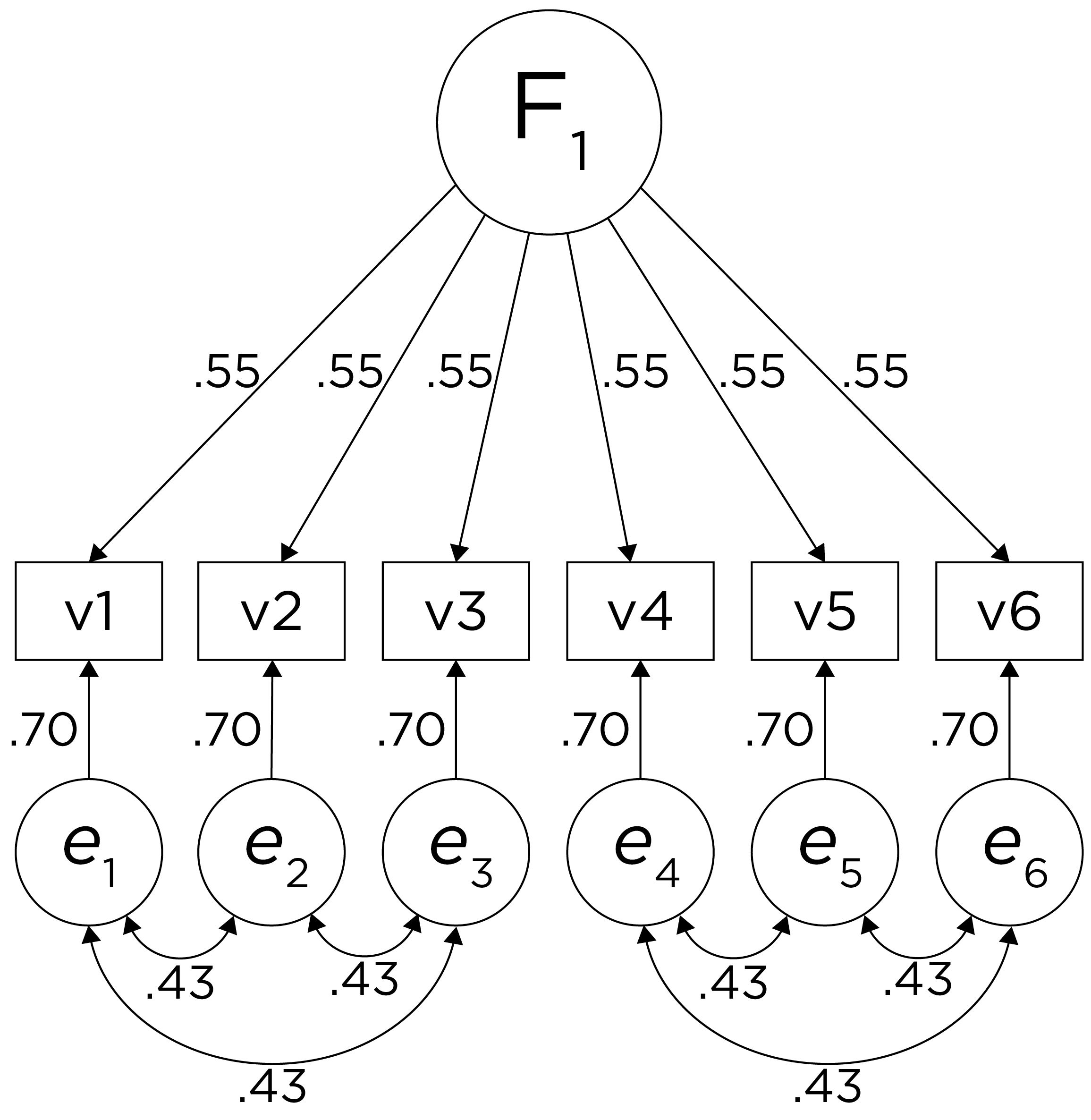
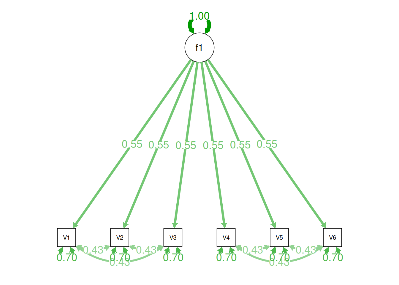
Alternatively, there could be a single factor that ties measures 1, 2, and 3 together and measures 4, 5, and 6 together, as depicted in Figure 14.11. In this model, the measures no longer have merely random error: measures 1, 2, and 3 have correlated residuals—that is, they share error variance (i.e., systematic error); likewise, measures 4, 5, and 6 have correlated residuals. This model has the exact same fit as the previous models. The amount of common variance (\(R^2\)) that is accounted for by an indicator is estimated as the square of the standardized loading: \(.30 = .55 \times .55\). The amount of error for an indicator is estimated as: \(\text{error} = 1 - \text{common variance}\), so in this case, the amount of error is: \(.70 = 1 - .30\). Using path tracing rules, the correlation of measures within a factor in this model is calculated as: \(.60 = (.55 \times .55) + (.70 \times .43 \times .70) + (.70 \times .43 \times .43 \times .70)\). The correlation of measures across factors in this model is calculated as: \(.30 = .55 \times .55\). In this model, the latent factor accounts for 30% of the variance in the indicators: \(\frac{.55^2 + .55^2 + .55^2 + .55^2 + .55^2 + .55^2}{6} = \frac{.30 + .30 + .30 + .30 + .30 + .30}{6} = .30\).
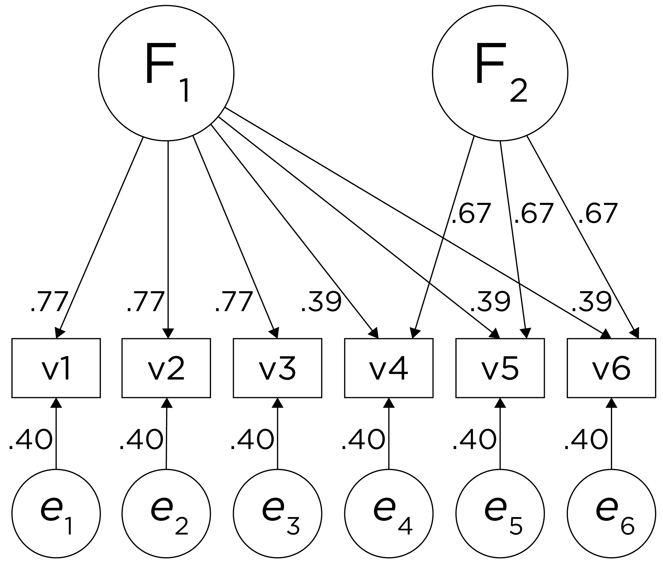
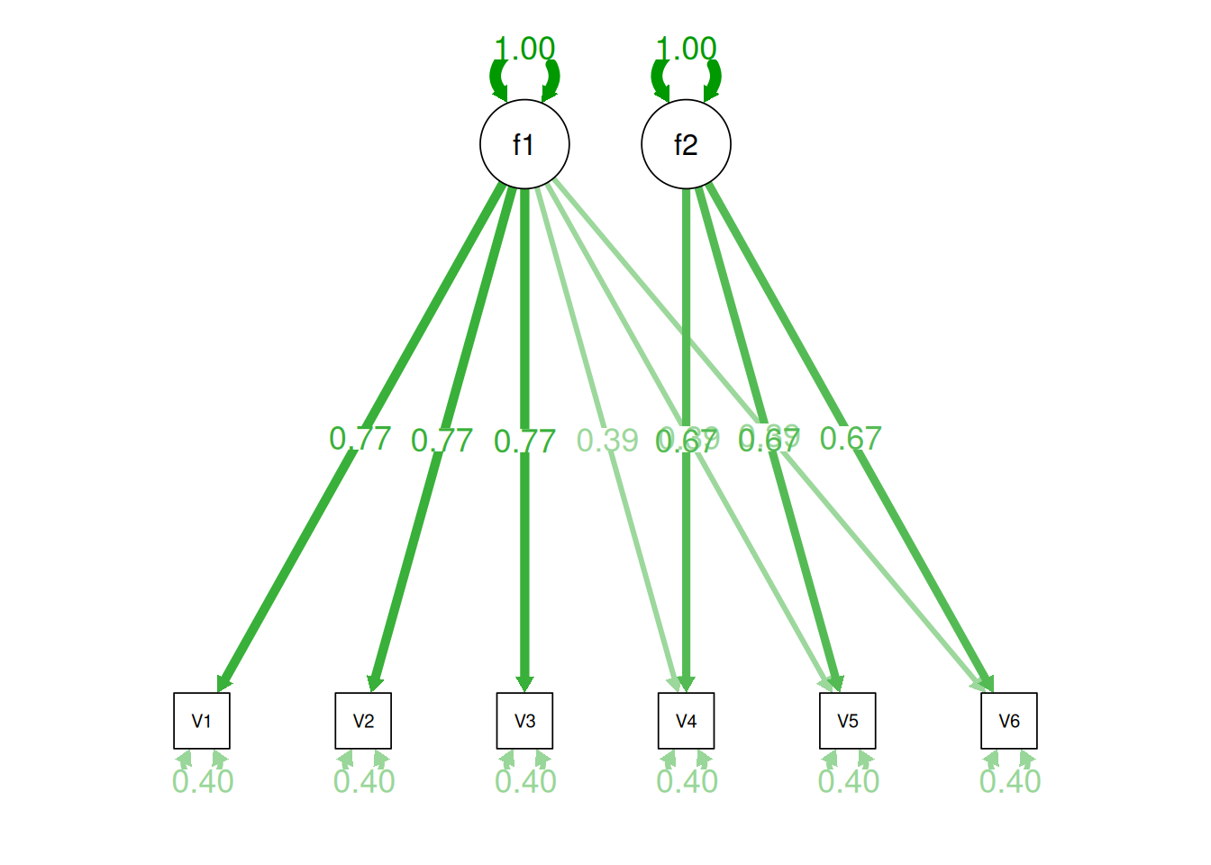
Alternatively, there could be a single factor that influences measures 1, 2, 3, 4, 5, and 6 in addition to a method bias factor (e.g., a particular measurement method, item stem, reverse-worded item, or another method bias) that influences measures 4, 5, and 6 equally, as depicted in Figure 14.12. In this model, measures 4, 5, and 6 have cross-loadings—that is, they load onto more than one latent factor. This model has the exact same fit as the previous models. The amount of common variance (\(R^2\)) that is accounted for by an indicator is estimated as the sum of the squared standardized loadings: \(.60 = .77 \times .77 = (.39 \times .39) + (.67 \times .67)\). The amount of error for an indicator is estimated as: \(\text{error} = 1 - \text{common variance}\), so in this case, the amount of error is: \(.40 = 1 - .60\). Using path tracing rules, the correlation of measures within a factor in this model is calculated as: \(.60 = (.77 \times .77) = (.39 \times .39) + (.67 \times .67)\). The correlation of measures across factors in this model is calculated as: \(.30 = .77 \times .39\). In this model, the first latent factor accounts for 37% of the variance in the indicators: \(\frac{.77^2 + .77^2 + .77^2 + .39^2 + .39^2 + .39^2}{6} = \frac{.59 + .59 + .59 + .15 + .15 + .15}{6} = .30\). The second latent factor accounts for 45% of the variance in its indicators: \(\frac{.67^2 + .67^2 + .67^2}{3} = \frac{.45 + .45 + .45}{3} = .45\).
Indeterminacy
There could be many more models that have the same fit to the data. Thus, factor analysis has indeterminacy because all of these models can explain these same data equally well, with all having different theoretical meaning. Factor indeterminacy reflects uncertainty (Rigdon et al., 2019a). The goal of factor analysis is for the model to look at the data and induce the model. However, most data matrices in real life are very complicated—much more complicated than in these examples.
This is why we do not calculate our own factor analysis by hand; use a stats program! It is important to think about the possibility of other models to determine how confident you can be in your data model. For every fully specified factor model—i.e., where the relevant paths are all defined, there is one and only one predictive data matrix (correlation matrix). However, each data matrix can produce many different factor models. Equivalent models are different models with the same degrees of freedom that have the same fit to the data—i.e., they generate the same model-implied covariance matrix and have the same fit indices. Rules for generating equivalent models are provided by Lee & Hershberger (1990). There is no way to distinguish which of these factor models is correct from the data matrix alone. Any given data matrix can predict an infinite number of factor models that accurately represent the data structure (Raykov & Marcoulides, 2001)—so we make decisions that determine what type of factor solution our data will yield. In general, factor indeterminacy—and the uncertainty it creates—tends to be greater in models with fewer items and where those items have smaller factor loadings and larger residual variances (Rigdon et al., 2019a). Conversely, factor indeterminacy is lower when there are many items per latent factor, and when loadings and factor correlations are strong (Rigdon et al., 2019b). Further, factor indeterminacy is compounded when creating factor scores for use in separate analyses (rather than estimating the associations within the same model; Rhemtulla & Savalei, 2025; Rigdon et al., 2019a). Thus, where possible, it is preferable to estimate associations between factors and other variables within the same model.
Many models could explain your data, and there are many more models that do not explain the data. For equally good-fitting models, decide based on interpretability. If you have strong theory, decide based on theory and things outside of factor analysis!
Practical Considerations
There are important considerations for doing factor analysis in real life with complex data. Traditionally, researchers had to consider what kind of data they have, and they often assumed interval-level data even though data in psychology are often not interval data. In the past, factor analysis was not good with categorical and dichotomous (e.g., True/False) data because the variance then is largely determined by the mean. So, we need something more complicated for dichotomous data. More solutions are available now for factor analysis with ordinal and dichotomous data, but it is generally best to have at least four ordered categories to perform factor analysis.
The necessary sample size depends on the complexity of the true factor structure. If there is a strong single factor for 30 items, then \(N = 50\) is plenty. But if there are five factors and some correlated errors, then the sample size will need to be closer to ~5,000. Factor analysis can recover the truth when the world is simple. However, nature is often not simple, and it may end in the distortion of nature instead of nature itself.
Recommendations for factor analysis are described by Sellbom & Tellegen (2019).
Decisions to Make in Factor Analysis
There are many decisions to make in factor analysis (Floyd & Widaman, 1995; Sarstedt et al., 2024). These decisions can have important impacts on the resulting solution. Decisions include things such as:
- What variables to include in the model and how to scale them
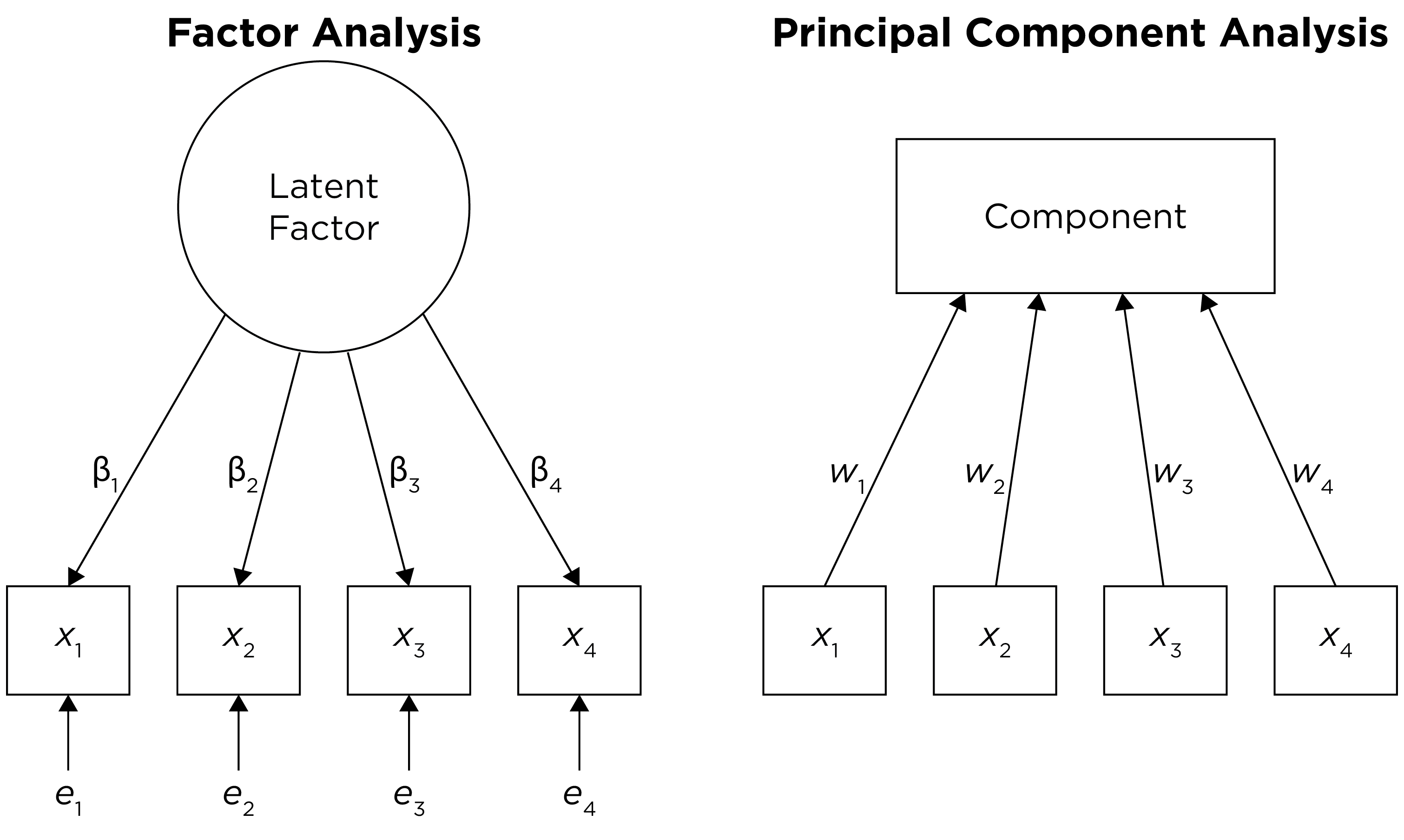
- Method of factor extraction: factor analysis or PCA
- If factor analysis, the kind of factor analysis: EFA or CFA
- How many factors to retain
- If EFA or PCA, whether and how to rotate factors (factor rotation)
- Model selection and interpretation
1. Variables to Include and their Scaling
The first decision when conducting a factor analysis is which variables to include and the scaling of those variables. What factors (or components) you extract can differ widely depending on what variables you include in the analysis. For example, if you include many variables from the same source (e.g., self-report), it is possible that you will extract a factor that represents the common variance among the variables from that source (i.e., the self-reported variables). This would be considered a method factor, which works against the goal of estimating latent factors that represent the constructs of interest (as opposed to the measurement methods used to estimate those constructs).
An additional consideration is the scaling of the variables. Before performing a PCA, it is generally important to ensure that the variables included in the PCA are on the same scale. PCA seeks to identify components that explain variance in the data, so if the variables are not on the same scale, some variables may contribute considerably more variance than others. A common way of ensuring that variables are on the same scale is to standardize them using, for example, z-scores that have a mean of zero and standard deviation of one. By contrast, factor analysis can better accommodate variables that are on different scales.
3. EFA or CFA
A third decision is the kind of factor analysis to use: exploratory factor analysis (EFA) or confirmatory factor analysis (CFA).
Exploratory Factor Analysis (EFA)
Exploratory factor analysis (EFA) is used if you have no a priori hypotheses about the factor structure of the model, but you would like to understand the latent variables represented by your items.
EFA is partly induced from the data. You feed in the data and let the program build the factor model. You can set some parameters going in, including how to extract or rotate the factors. The factors are extracted from the data without specifying the number and pattern of loadings between the items and the latent factors (Bollen, 2002). All cross-loadings are freely estimated.
Confirmatory Factor Analysis (CFA)
Confirmatory factor analysis (CFA) is used to (dis)confirm a priori hypotheses about the factor structure of the model. CFA is a test of the hypothesis. In CFA, you specify the model and ask how well this model represents the data. The researcher specifies the number, meaning, associations, and pattern of free parameters in the factor loading matrix (Bollen, 2002). A key advantage of CFA is the ability to directly compare alternative models (i.e., factor structures), which is valuable for theory testing (Strauss & Smith, 2009). For instance, you could use CFA to test whether the variance in several measures’ scores is best explained with one factor or two factors. In CFA, cross-loadings are not estimated unless the researcher specifies them.
Exploratory Structural Equation Modeling (ESEM)
In real life, there is not a clear distinction between EFA and CFA. In CFA, researchers often set only half of the constraints, and let the data fill in the rest. Moreover, our initial hypothesized CFA model is often not a good fit to the data—especially for models with many items (Floyd & Widaman, 1995)—and requires modification for adequate fit, such as cross loadings and correlated residuals. Such modifications are often made based on empirical criteria (e.g., modification indices) rather than our initial hypothesis. In EFA, researchers often set constraints and assumptions. Moreover, the initial items for the EFA were selected by the researcher, who often has expectations about the number and types of factors that will be extracted. Thus, the line between EFA and CFA is often blurred. There is an exploratory–confirmatory continuum, and the important thing is to report which aspects of your modeling approach were exploratory and which were confirmatory.
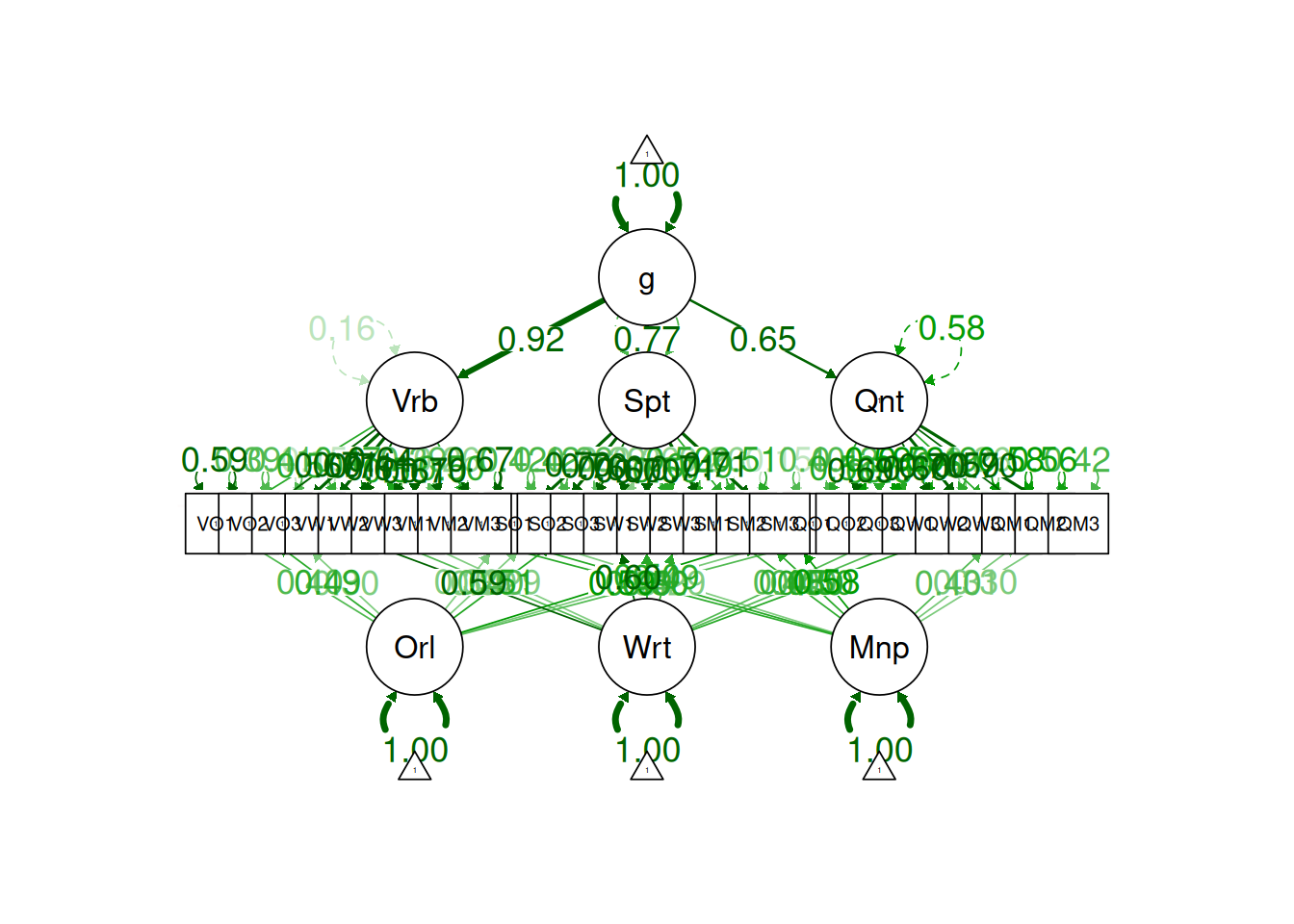
EFA and CFA can be considered special cases of exploratory structural equation modeling (ESEM), which combines features of EFA, CFA, and SEM (Marsh et al., 2014). ESEM can include any combination of exploratory (i.e., EFA) and confirmatory (CFA) factors. ESEM, unlike traditional CFA models, typically estimates all cross-loadings—at least for the exploratory factors. If a CFA model without cross-loadings and correlated residuals fits as well as an ESEM model with all cross-loadings, the CFA model should be retained for its simplicity. However, ESEM models often fit better than CFA models because requiring no cross-loadings is an unrealistic expectation of items from many psychological instruments (Marsh et al., 2014). The correlations between factors tend to be positively biased when fitting CFA models without cross-loadings, which leads to challenges in using CFA to establish discriminant validity (Marsh et al., 2014). Thus, compared to CFA, ESEM has the potential to more accurately estimate factor correlations and establish discriminant validity (Marsh et al., 2014). Moreover, ESEM can be useful in a multitrait-multimethod framework. We provide examples of ESEM in Section 14.4.3.
4. How Many Factors to Retain
A goal of factor analysis and PCA is simplification or parsimony, while still explaining as much variance as possible. The hope is that you can have fewer factors that explain the associations between the variables than the number of observed variables. The fewer the number of factors retained, the greater the parsimony, but the greater the amount of information that is discarded (i.e., the less the variance accounted for in the variables). The more factors we retain, the less the amount of information that is discarded (i.e., more variance is accounted for in the variables), but the less the parsimony. But how do you decide on the number of factors (in factor analysis) or components (in PCA)?
There are a number of criteria that one can use to help determine how many factors/components to keep:
- Kaiser-Guttman criterion (Kaiser, 1960): in PCA, components with eigenvalues greater than 1
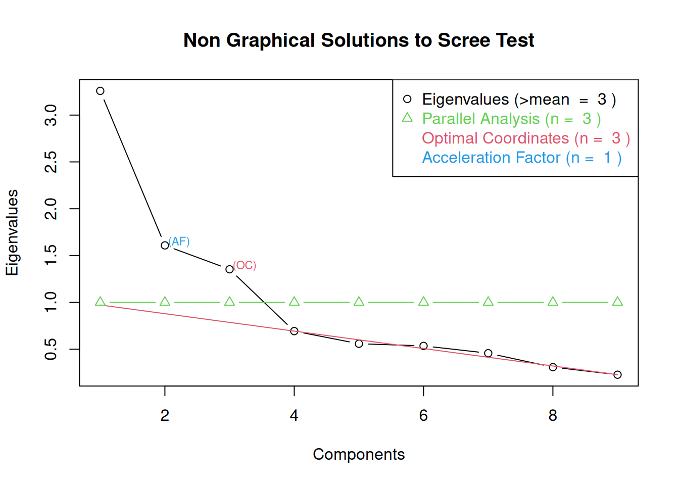
- Cattell’s scree test (Cattell, 1966): the “elbow” (inflection point) in a scree plot minus one; sometimes operationalized with optimal coordinates (OC) or the acceleration factor (AF)
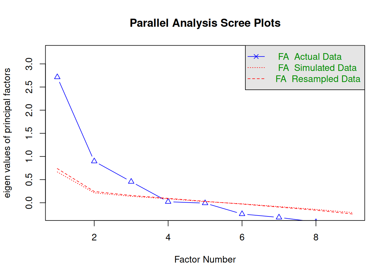
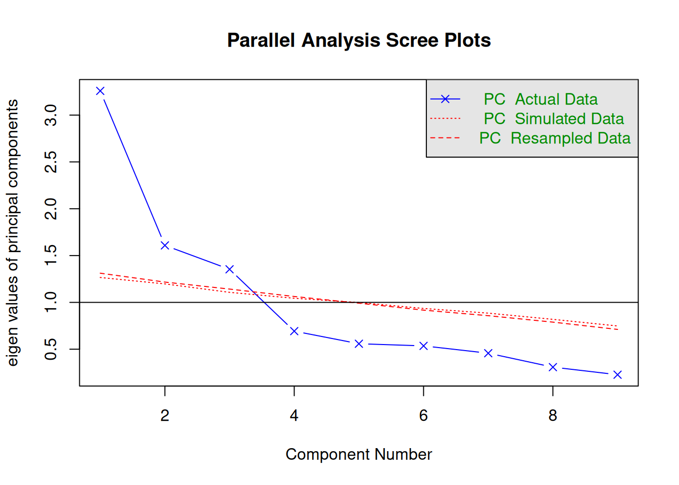
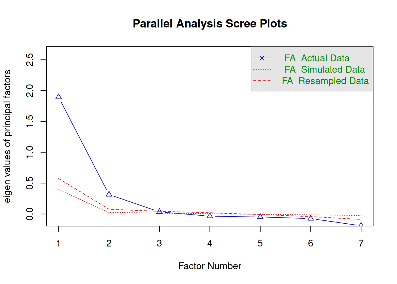
- Parallel analysis: factors that explain more variance than randomly simulated data
-
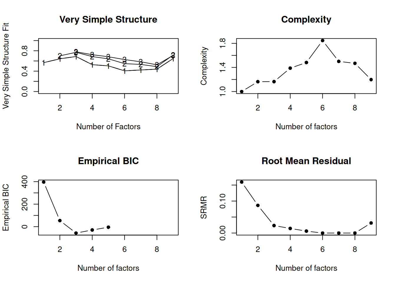
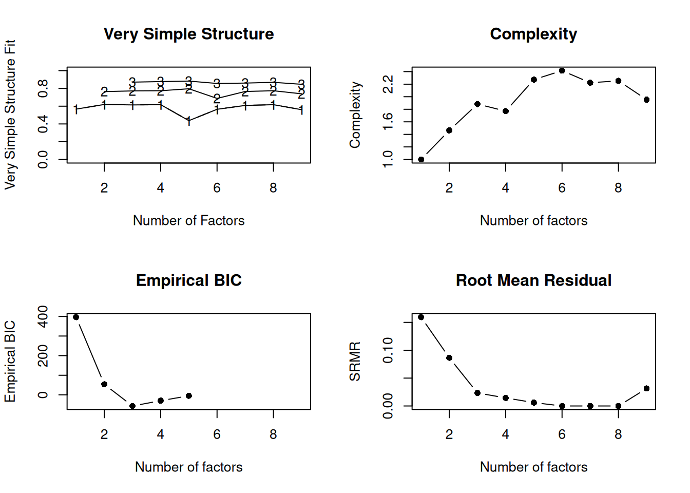
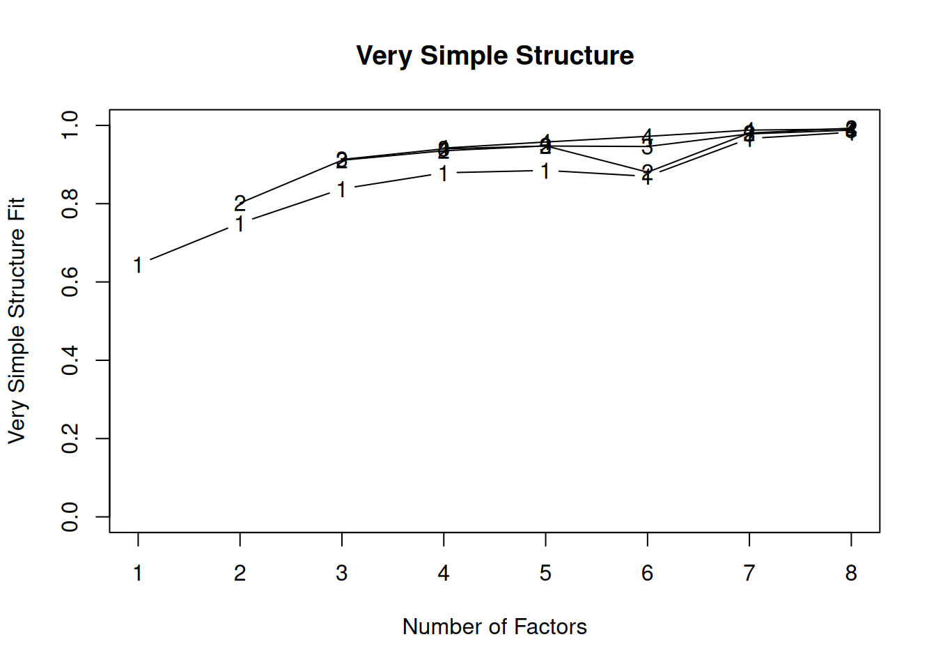
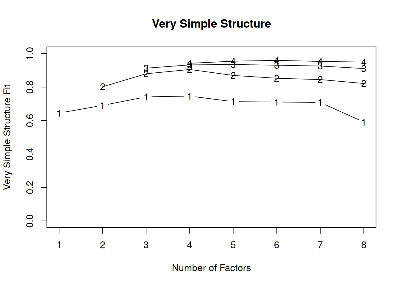
Very simple structure (VSS) criterion: larger is better
- Velicer’s minimum average partial (MAP) test: smaller is better
- Akaike information criterion (AIC): smaller is better
- Bayesian information criterion (BIC): smaller is better
- Sample size-adjusted BIC (SABIC): smaller is better
- Root mean square error of approximation (RMSEA): smaller is better
- Chi-square difference test: smaller is better; a significant test indicates that the more complex model is significantly better fitting than the less complex model
- Standardized root mean square residual (SRMR): smaller is better
- Comparative Fit Index (CFI): larger is better
- Tucker Lewis Index (TLI): larger is better
There is not necessarily a “correct” criterion to use in determining how many factors to keep, so it is generally recommended that researchers use multiple criteria in combination with theory and interpretability.
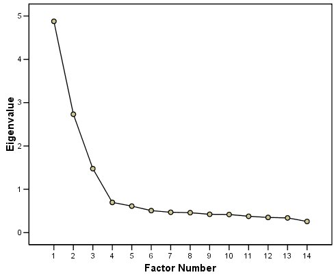
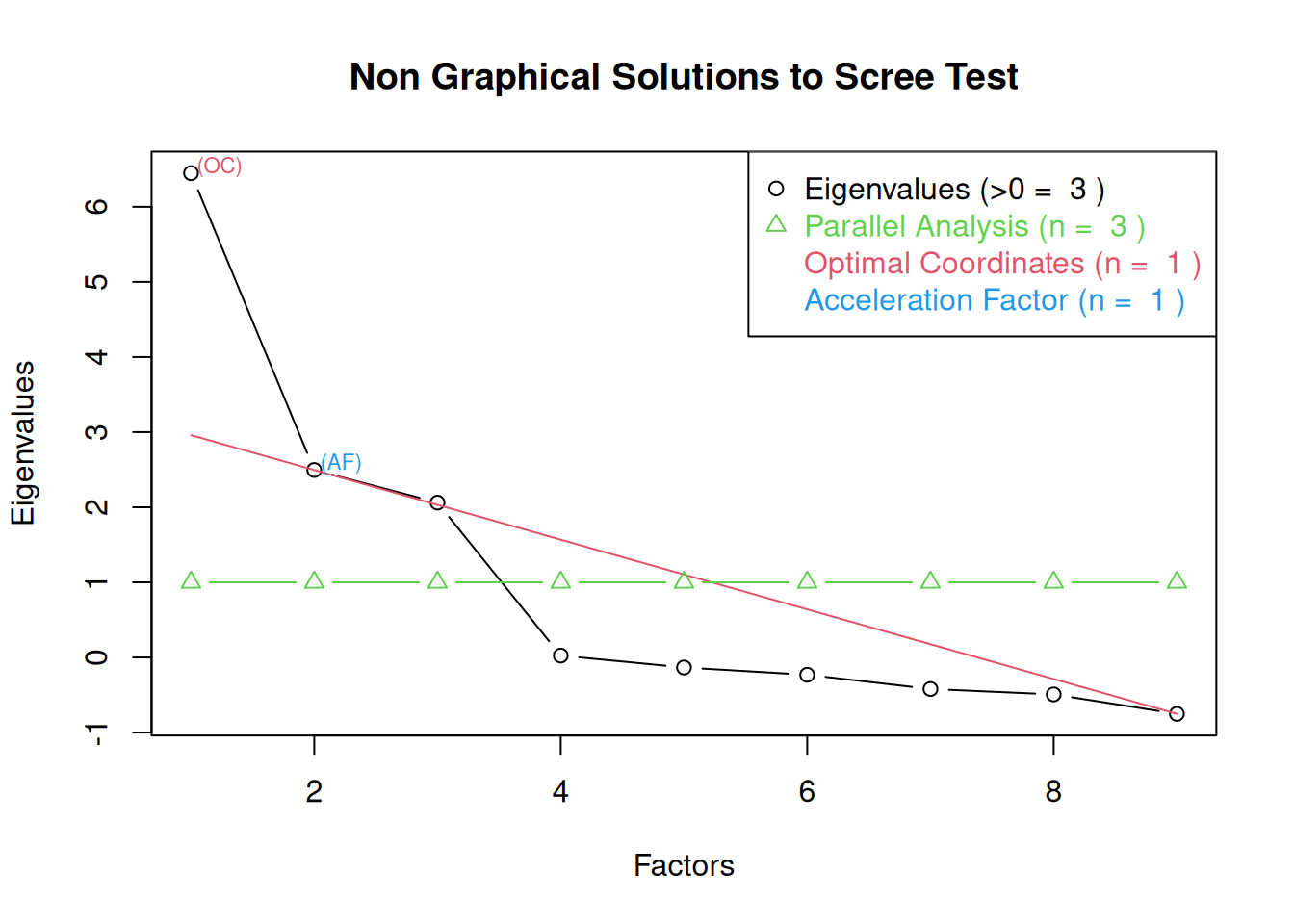
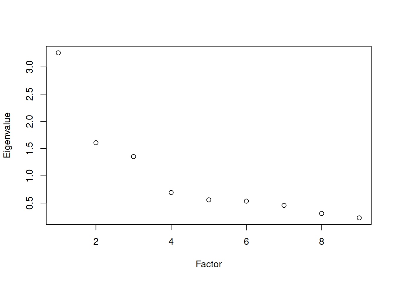
A scree plot from a factor analysis or PCA provides lots of information. A scree plot has the factor number on the x-axis and the eigenvalue on the y-axis. The eigenvalue is the variance accounted for by a factor; when using a varimax (orthogonal) rotation, an eigenvalue (or factor variance) is calculated as the sum of squared standardized factor (or component) loadings on that factor. An example of a scree plot is in Figure 14.14.
The total variance is equal to the number of variables you have, so one eigenvalue is approximately one variable’s worth of variance. In a factor analysis and PCA, the first factor (or component) accounts for the most variance, the second factor accounts for the second-most variance, and so on. The more factors you add, the less variance is explained by the additional factor.
One criterion for how many factors to keep is the Kaiser-Guttman criterion. According to the Kaiser-Guttman criterion (Kaiser, 1960), you should keep any factors whose eigenvalue is greater than 1. That is, for the sake of simplicity, parsimony, and data reduction, you should take any factors that explain more than a single variable would explain. According to the Kaiser-Guttman criterion, we would keep three factors from Figure 14.14 that have eigenvalues greater than 1. The default in SPSS is to retain factors with eigenvalues greater than 1. However, keeping factors whose eigenvalue is greater than 1 is not the most correct rule. If you let SPSS do this, you may get many factors with eigenvalues around 1 (e.g., factors with an eigenvalue ~ 1.0001) that are not adding so much that it is worth the added complexity. The Kaiser-Guttman criterion usually results in keeping too many factors. Factors with small eigenvalues around 1 could reflect error shared across variables. For instance, factors with small eigenvalues could reflect method variance (i.e., method factor), such as a self-report factor that turns up as a factor in factor analysis, but that may be useless to you as a conceptual factor of a construct of interest.
Another criterion is Cattell’s scree test (Cattell, 1966), which involves selecting the number of factors from looking at the scree plot. “Scree” refers to the rubble of stones at the bottom of a mountain. According to Cattell’s scree test, you should keep the factors before the last steep drop in eigenvalues—i.e., the factors before the rubble, where the slope approaches zero. The beginning of the scree (or rubble), where the slope approaches zero, is called the “elbow” of a scree plot. Using Cattell’s scree test, you retain the number of factors that explain the most variance prior to the explained variance drop-off, because, ultimately, you want to include only as many factors in which you gain substantially more by the inclusion of these factors. That is, you would keep the number of factors at the elbow of the scree plot minus one. If the last steep drop occurs from Factor 4 to Factor 5 and the elbow is at Factor 5, we would keep four factors. In Figure 14.14, the last steep drop in eigenvalues occurs from Factor 3 to Factor 4; the elbow of the scree plot occurs at Factor 4. We would keep the number of factors at the elbow minus one. Thus, using Cattell’s scree test, we would keep three factors based on Figure 14.14.
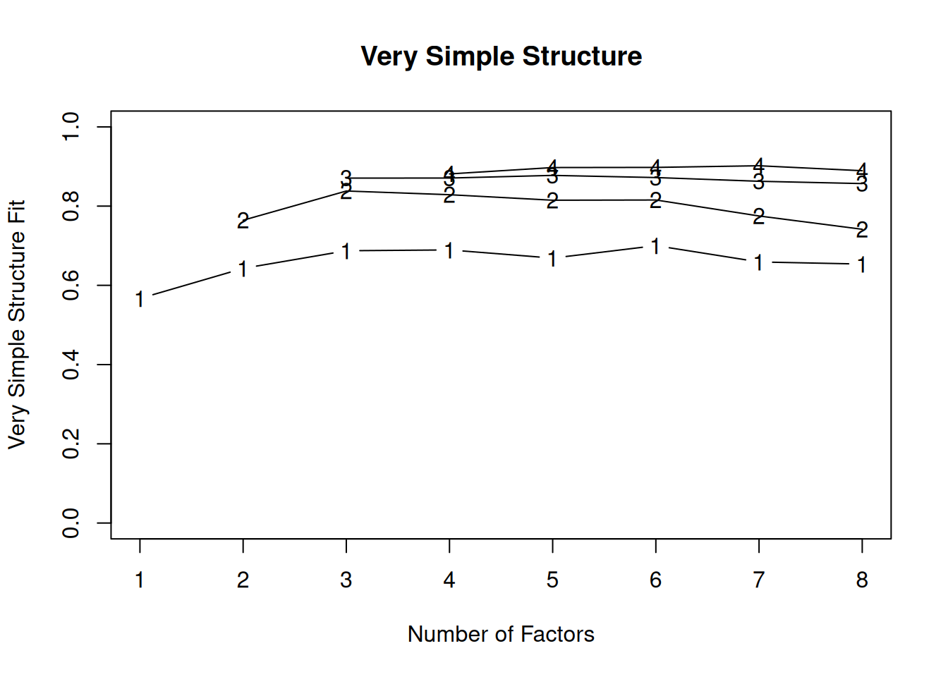
There are more sophisticated ways of using a scree plot, but they usually end up at a similar decision. Examples of more sophisticated tests include parallel analysis and very simple structure (VSS) plots. In a parallel analysis, you examine where the eigenvalues from observed data and random data converge, so you do not retain a factor that explains less variance than would be expected by random chance. A parallel analysis can be helpful when you have many variables and one factor accounts for the majority of the variance such that the elbow is at Factor 2 (which would result in keeping one factor), but you have theoretical reasons to select more than one factor. An example in which parallel analysis may be helpful is with neurophysiological data. For instance, parallel analysis can be helpful when conducting temporo-spatial PCA of event-related potential (ERP) data in which you want to separate multiple time windows and multiple spatial locations despite a predominant signal during a given time window and spatial location (Dien, 2012).
In general, my recommendation is to use Cattell’s scree test, and then test the factor solutions with plus or minus one factor. You should never accept PCA components with eigenvalues less than one (or factors with eigenvalues less than zero), because they are likely to be largely composed of error. If you are using maximum likelihood factor analysis, you can compare the fit of various models with model fit criteria to see which model fits best for its parsimony. A model will always fit better when you add additional parameters or factors, so you examine if there is significant improvement in model fit when adding the additional factor—that is, we keep adding complexity until additional complexity does not buy us much. Always try a factor solution that is one less and one more than suggested by Cattell’s scree test to buffer your final solution because the purpose of factor analysis is to explain things and to have interpretability. Even if all rules or indicators suggest to keep X number of factors, maybe \(\pm\) one factor helps clarify things. Even though factor analysis is empirical, theory and interpretatability should also inform decisions.
5. Factor Rotation
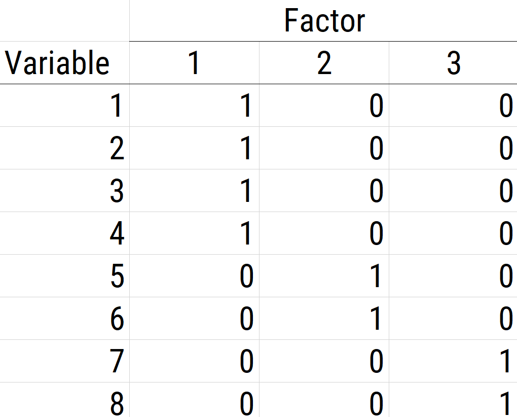
The next step if using EFA or PCA is, possibly, to rotate the factors to make them more interpretable and simple, which is the whole goal. To interpret the results of a factor analysis, we examine the factor matrix. The columns refer to the different factors; the rows refer to the different observed variables. The cells in the table are the factor loadings—they are basically the correlation between the variable and the factor. Our goal is to achieve a model with simple structure because it is easily interpretable. Simple structure means that every variable loads perfectly on one and only one factor, as operationalized by a matrix of factor loadings with values of one and zero and nothing else. An example of a factor matrix that follows simple structure is depicted in Figure 14.15.
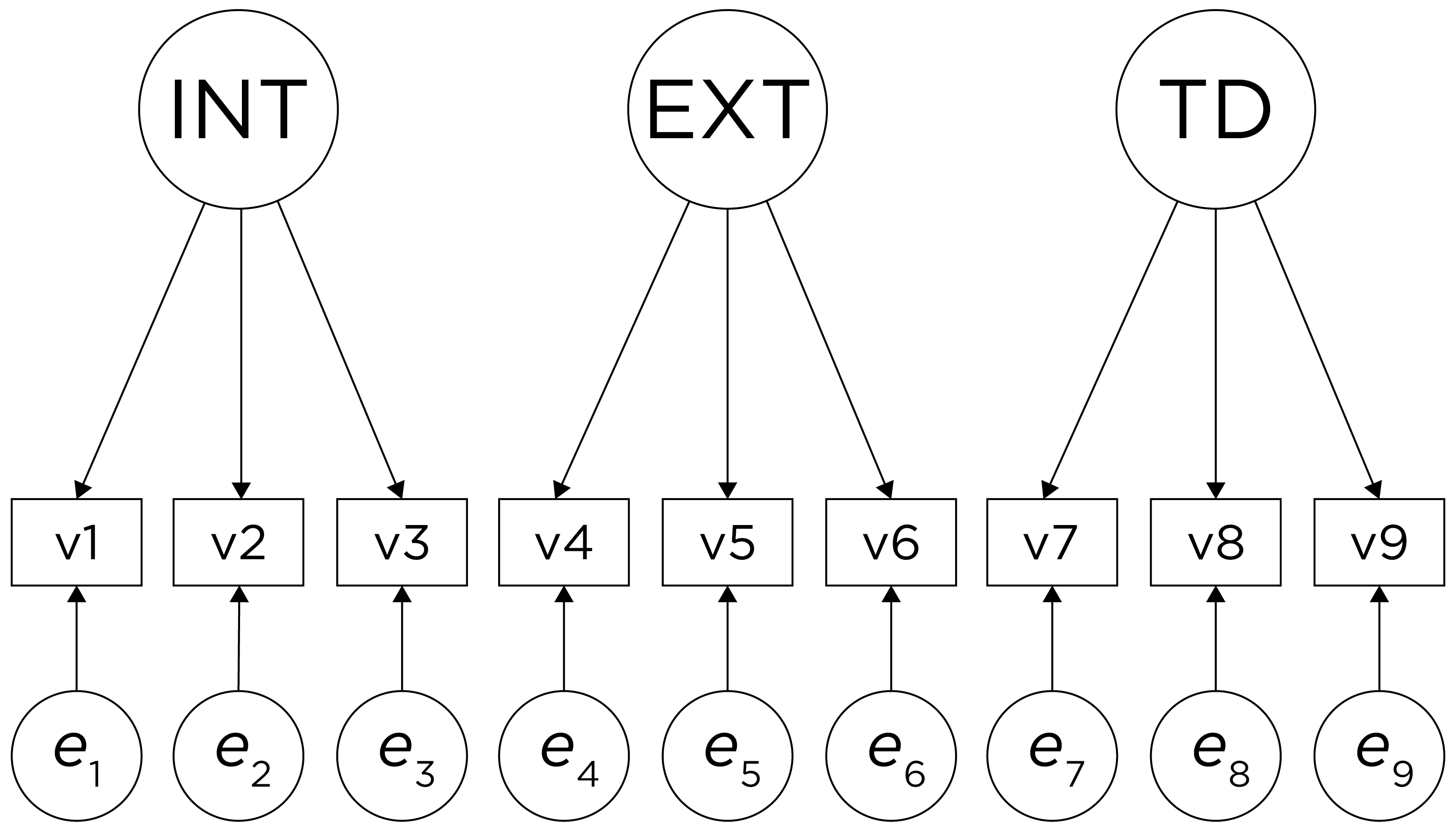
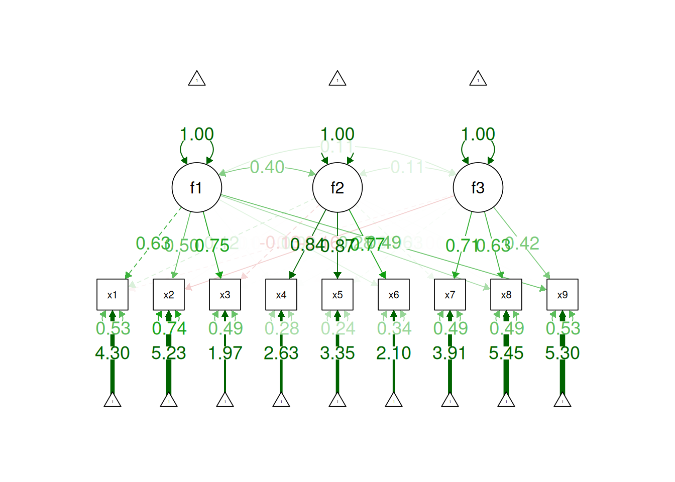
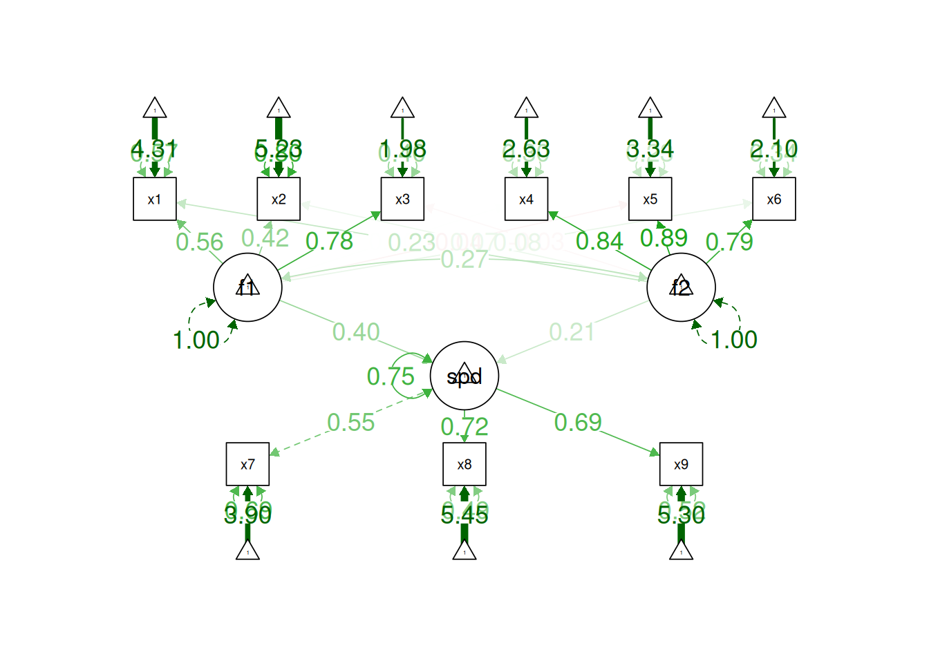
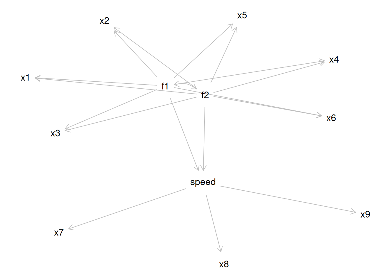
An example of a measurement model that follows simple structure is depicted in Figure 14.16. Each variable loads onto one and only one factor, which makes it easy to interpret the meaning of each factor, because a given factor represents the common variance among the items that load onto it.
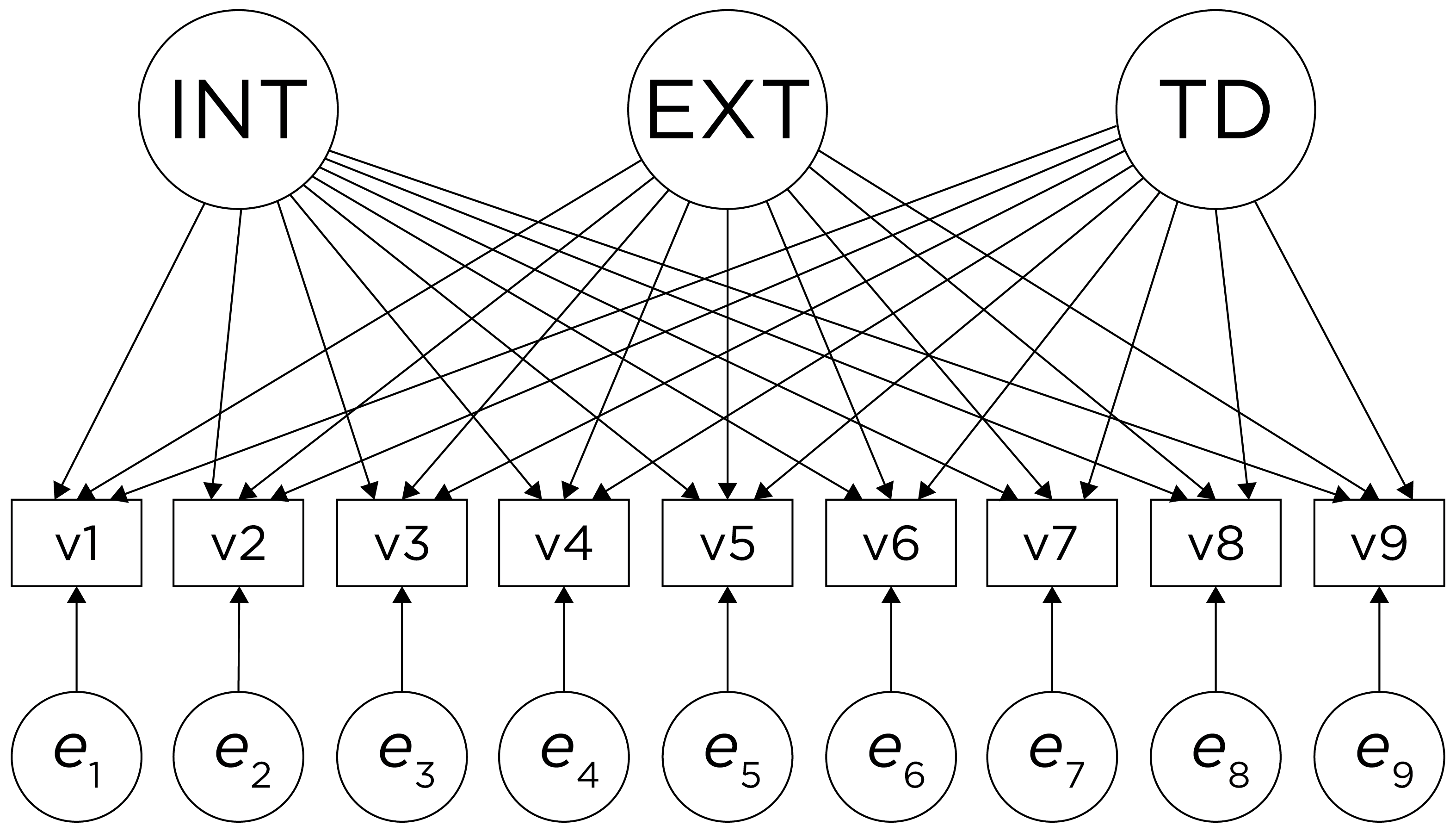
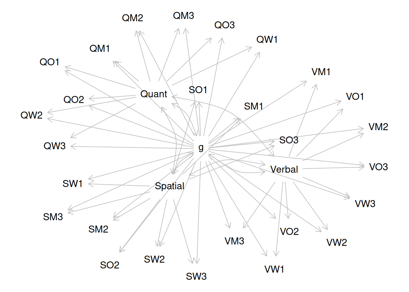
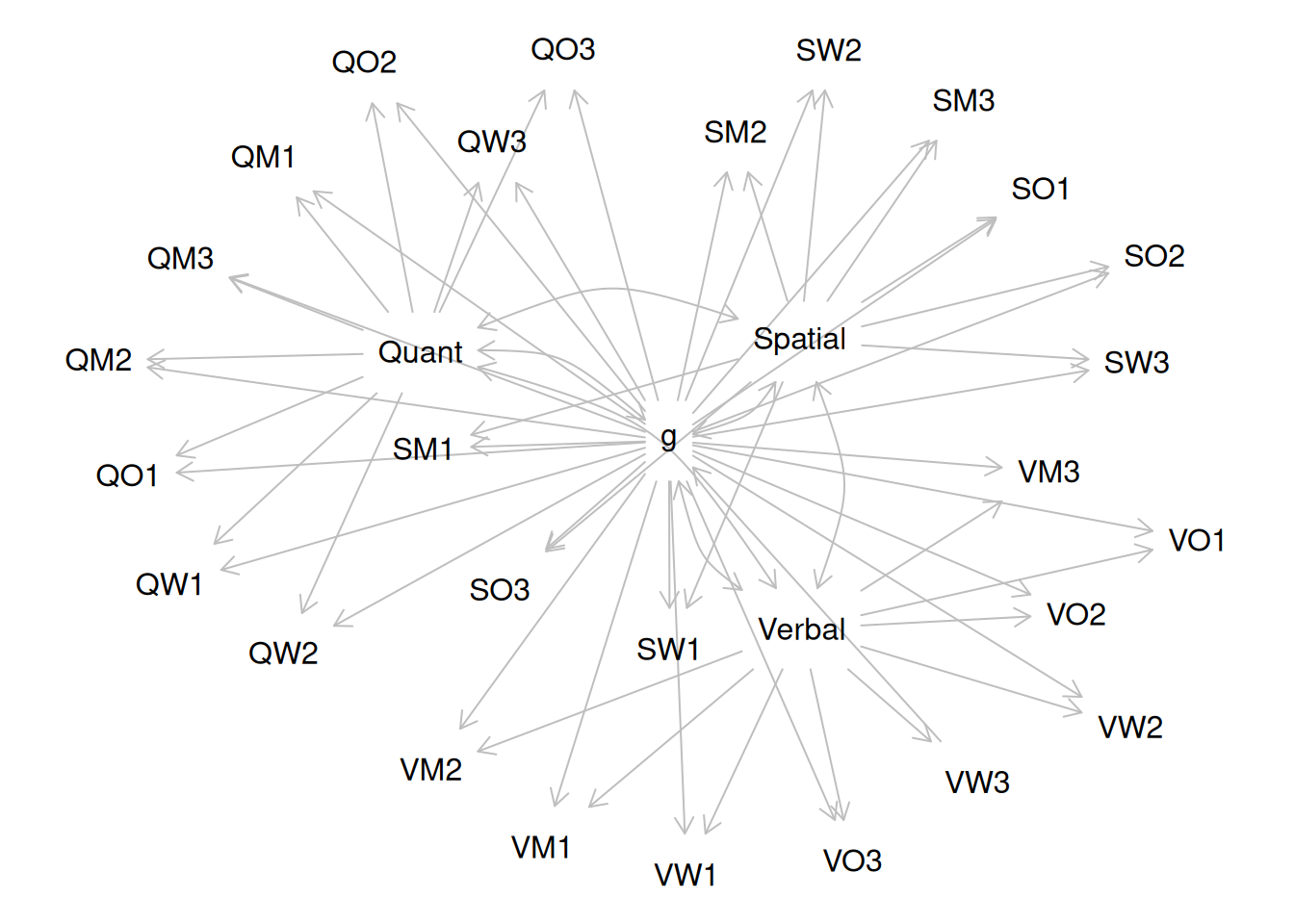
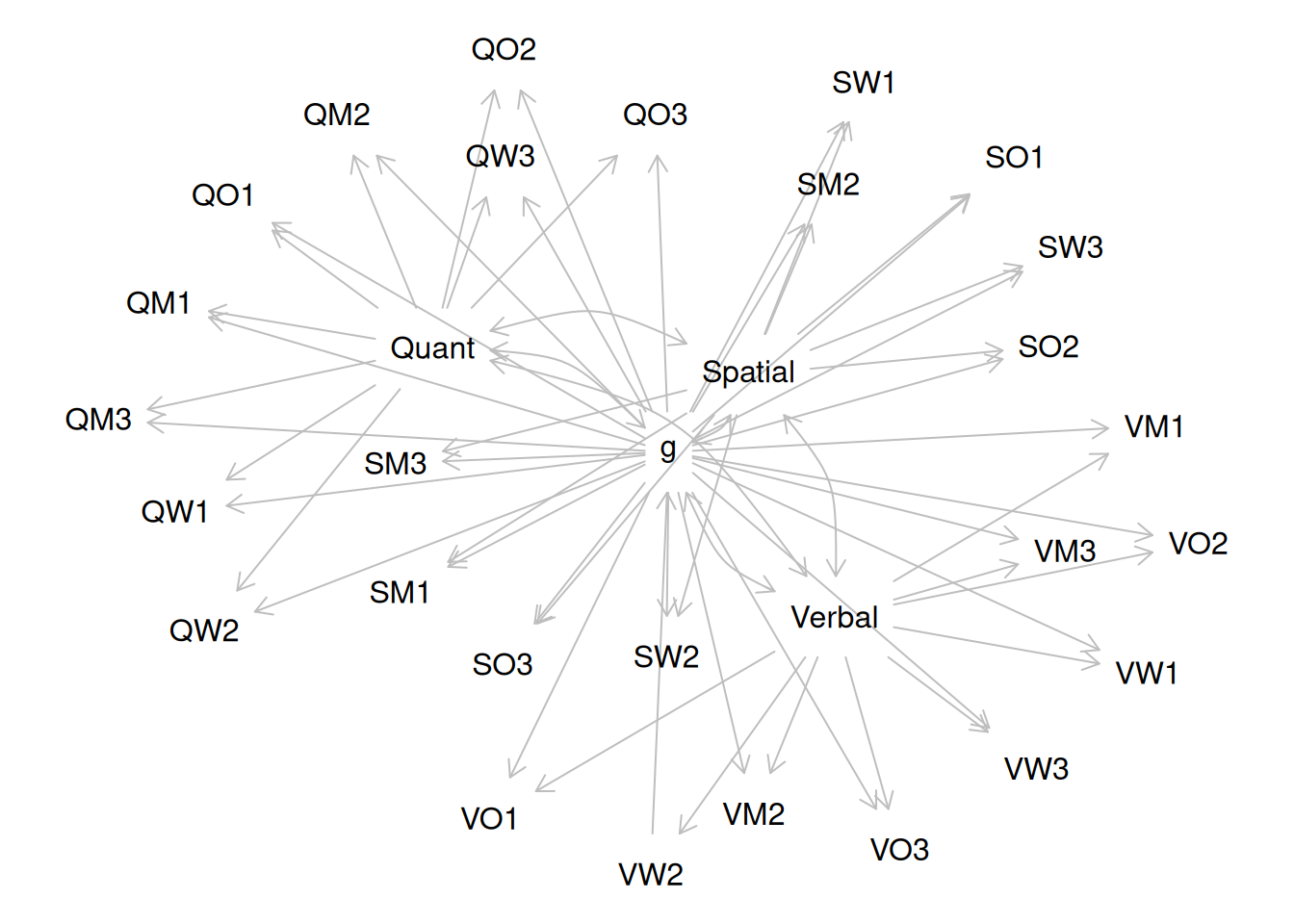
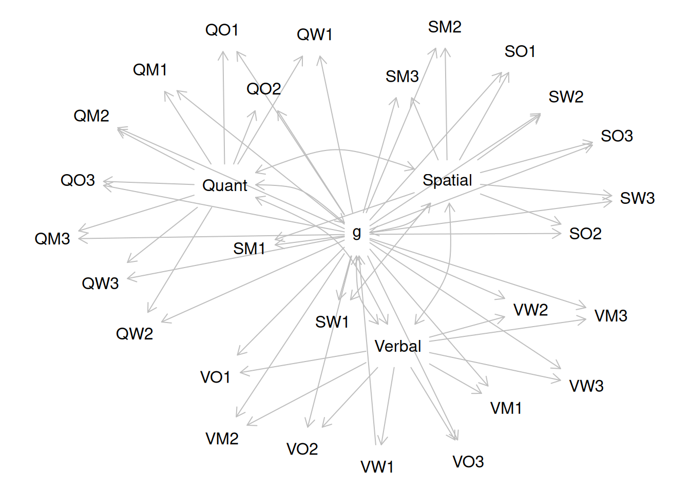
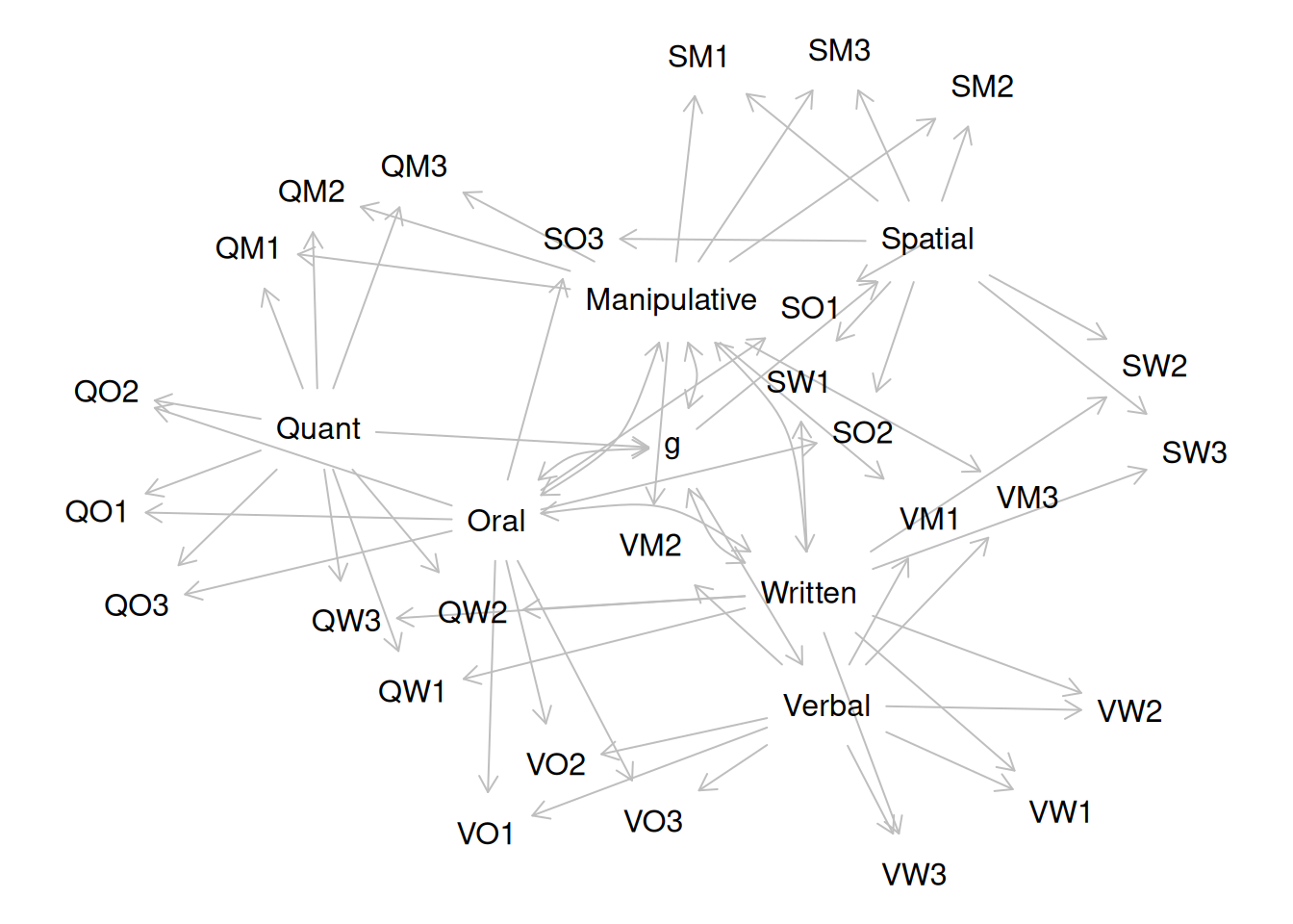
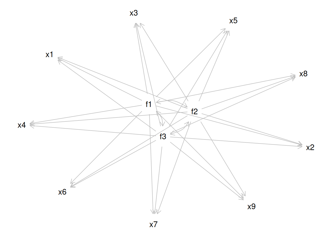
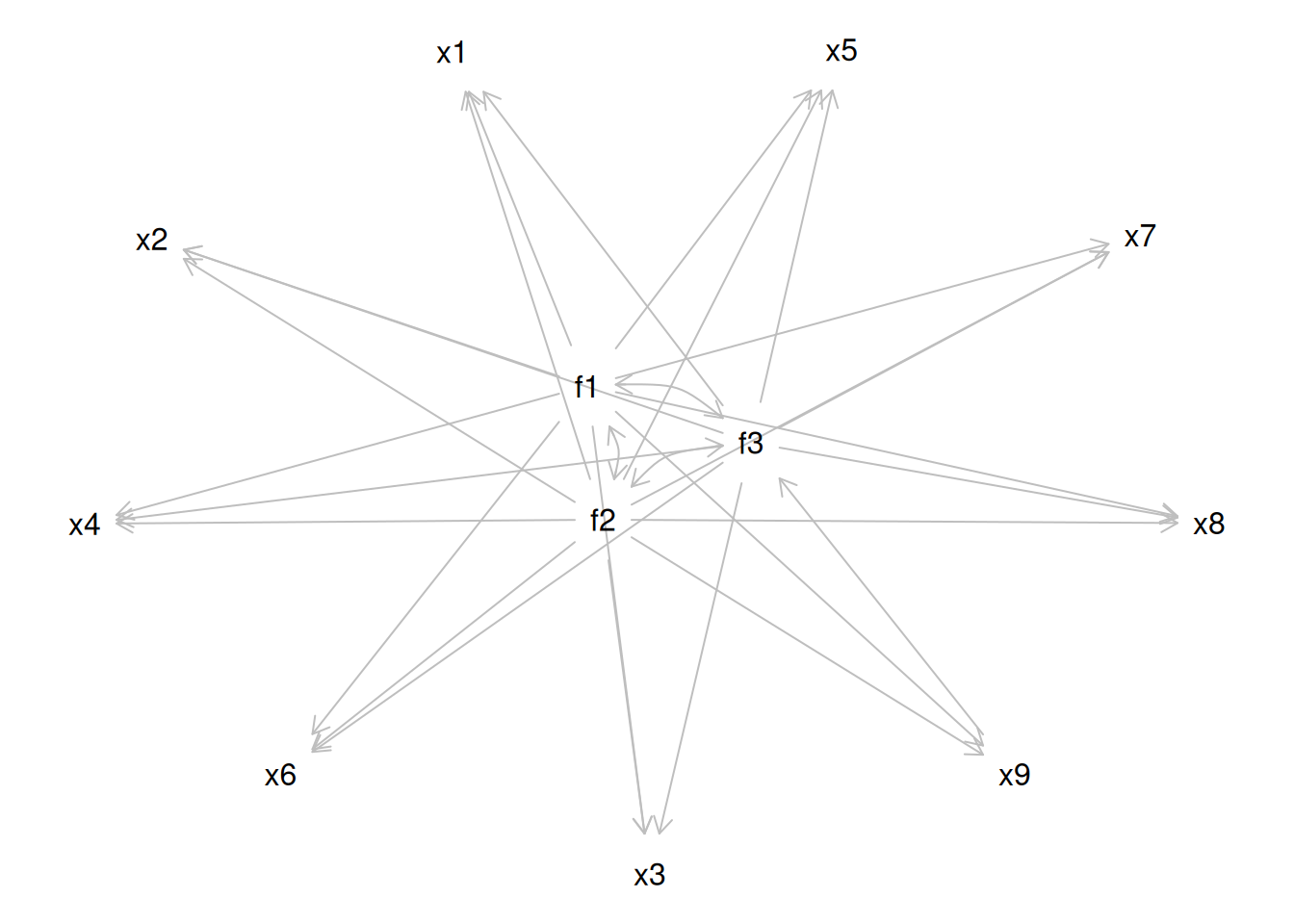
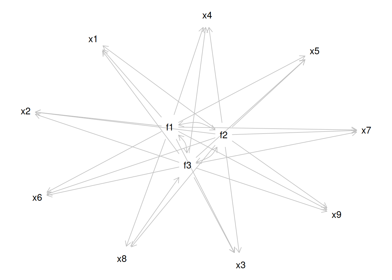
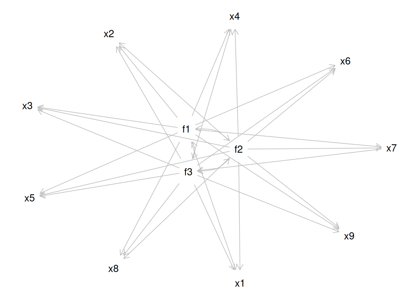
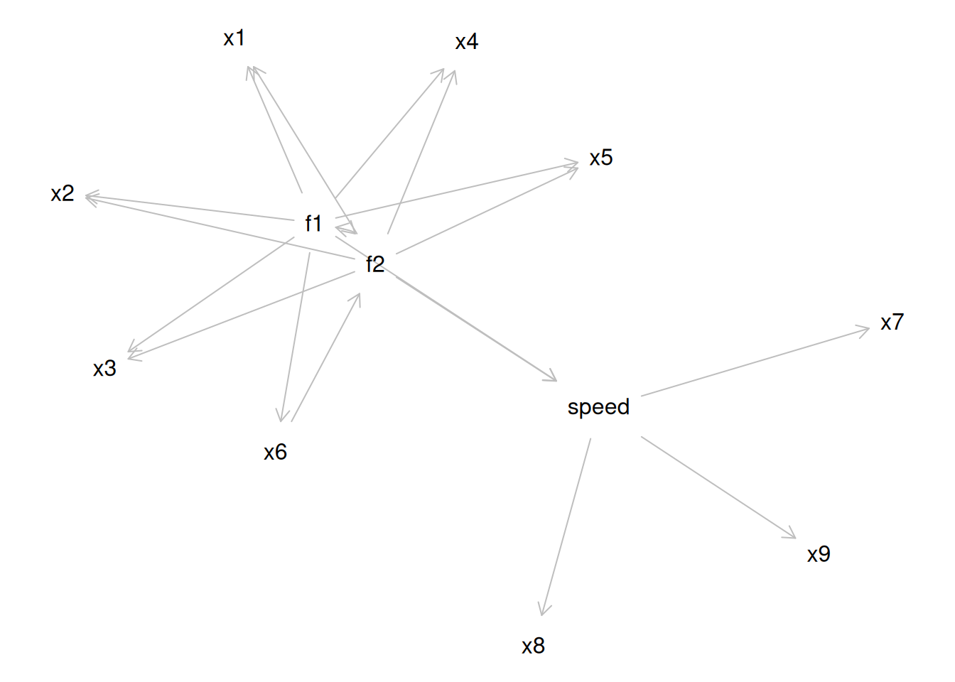
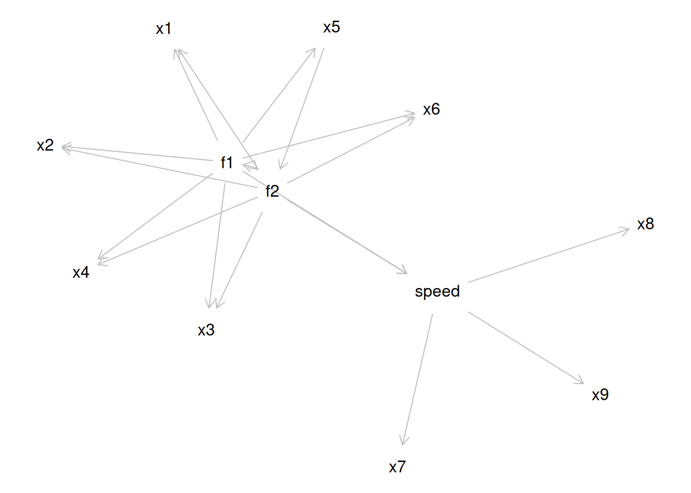
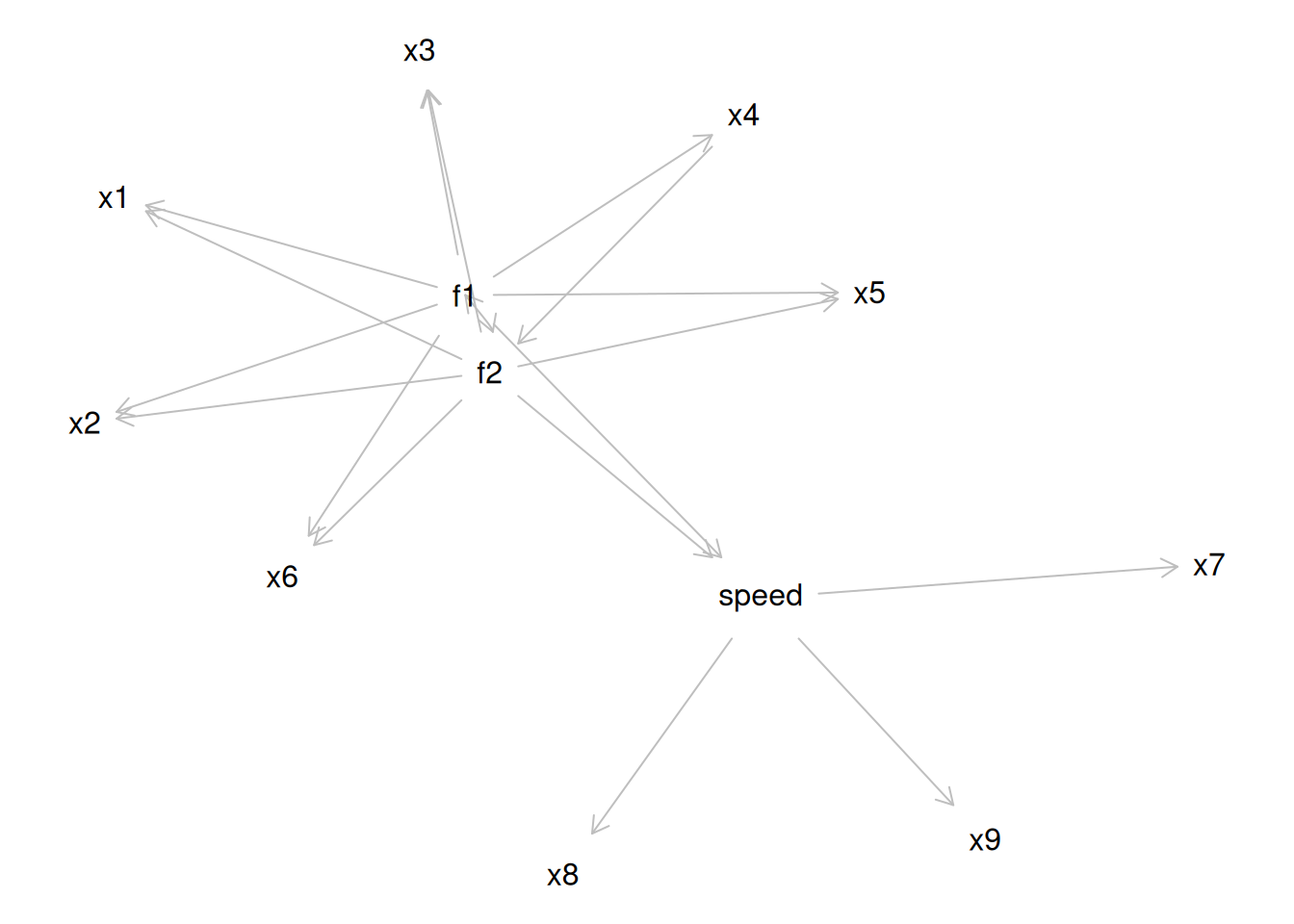
However, pure simple structure only occurs in simulations, not in real-life data. In reality, our measurement model in an unrotated factor analysis model might look like the model in Figure 14.17. In this example, the measurement model does not show simple structure because the items have cross-loadings—that is, the items load onto more than one factor. The cross-loadings make it difficult to interpret the factors, because all of the items load onto all of the factors, so the factors are not very distinct from each other, which makes it difficult to interpret what the factors mean.
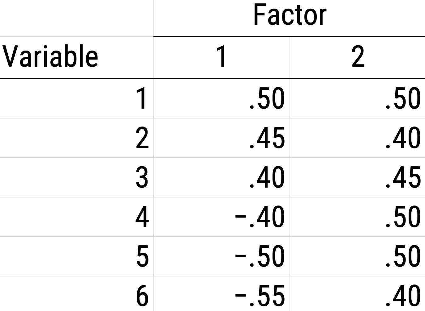
As a result of the challenges of interpretability caused by cross-loadings, factor rotations are often performed. An example of an unrotated factor matrix is in Figure 14.18.
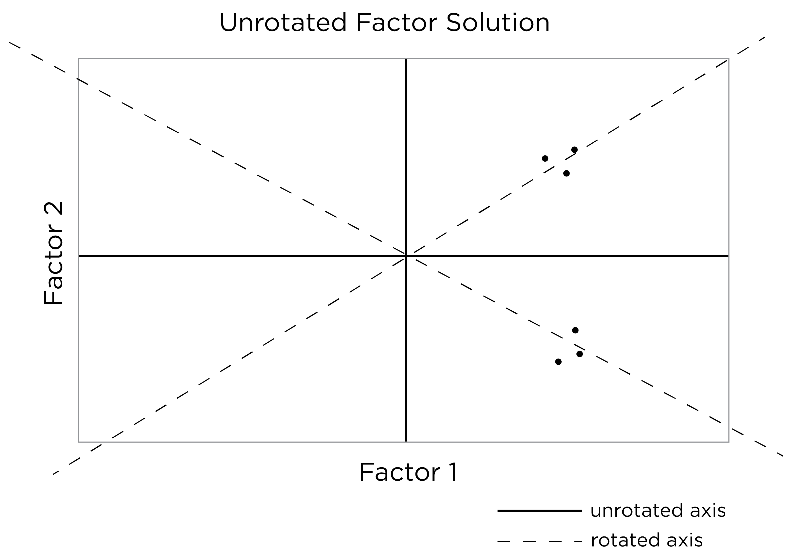
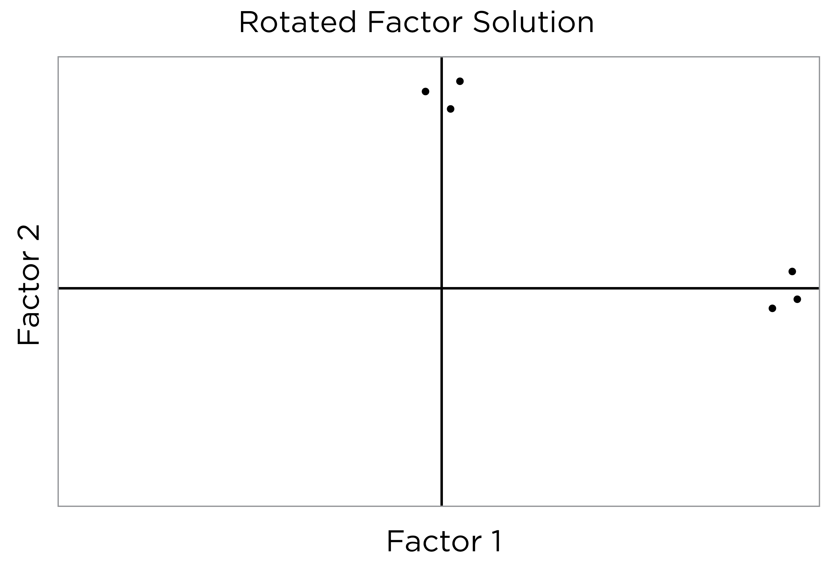
In the example factor matrix in Figure 14.18, the factor analysis is not very helpful—it tells us very little because it did not distinguish between the two factors. The variables have similar loadings on Factor 1 and Factor 2. An example of a unrotated factor solution is in Figure 14.19. In the figure, all of the variables are in the midst of the quadrants—they are not on the factors’ axes. Thus, the factors are not very informative.
As a result, to improve the interpretability of the factor analysis, we can do what is called rotation. Rotation leverages the idea that there are infinite solutions to the factor analysis model that fit equally well. Rotation involves changing the orientation of the factors by changing the axes so that variables end up with very high (close to one or negative one) or very low (close to zero) loadings, so that it is clear which factors include which variables (and which factors each variable most strongly loads onto). That is, rotation rescales the factors and tries to identify the ideal solution (factor) for each variable. Rotation occurs by changing the variables’ loadings while keeping the structure of correlations among the variables intact (Field et al., 2012). Moreover, rotation does not change the variance explained by factors. Rotation searches for simple structure and keeps searching until it finds a minimum (i.e., the closest as possible to simple structure). After rotation, if the rotation was successful for imposing simple structure, each factor will have loadings close to one (or negative one) for some variables and close to zero for other variables. The goal of factor rotation is to achieve simple structure, to help make it easier to interpret the meaning of the factors.
To perform factor rotation, orthogonal rotations are often used. Orthogonal rotations make the rotated factors uncorrelated. An example of a commonly used orthogonal rotation is varimax rotation. Varimax rotation maximizes the sum of the variance of the squared loadings (i.e., so that items have either a very high or very low loading on a factor) and yields axes with a 90-degree angle.
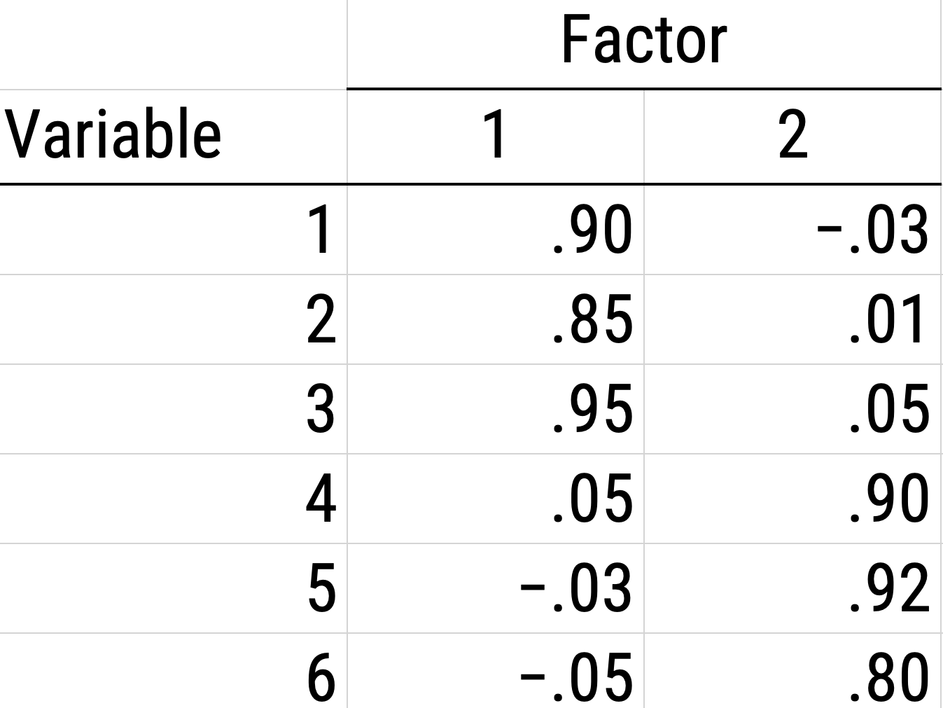
An example of a factor matrix following an orthogonal rotation is depicted in Figure 14.20. An example of a factor solution following an orthogonal rotation is depicted in Figure 14.21.
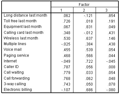
An example of a factor matrix from SPSS following an orthogonal rotation is depicted in Figure 14.22.
An example of a factor structure from an orthogonal rotation is in Figure 14.23.
Sometimes, however, the two factors and their constituent variables may be correlated. Examples of two correlated factors may be depression and anxiety. When the two factors are correlated in reality, if we make them uncorrelated, this would result in an inaccurate model. Oblique rotation allows for factors to be correlated and yields axes with an angle of less than 90 degrees. However, if the factors have low correlation (e.g., .2 or less), you can likely continue with orthogonal rotation. Nevertheless, just because an oblique rotation allows for correlated factors does not mean that the factors will be correlated, so oblique rotation provides greater flexibility than orthogonal rotation. An example of a factor structure from an oblique rotation is in Figure 14.24. Results from an oblique rotation are more complicated than orthogonal rotation—they provide lots of output and are more complicated to interpret. In addition, oblique rotation might not yield a smooth answer if you have a relatively small sample size.
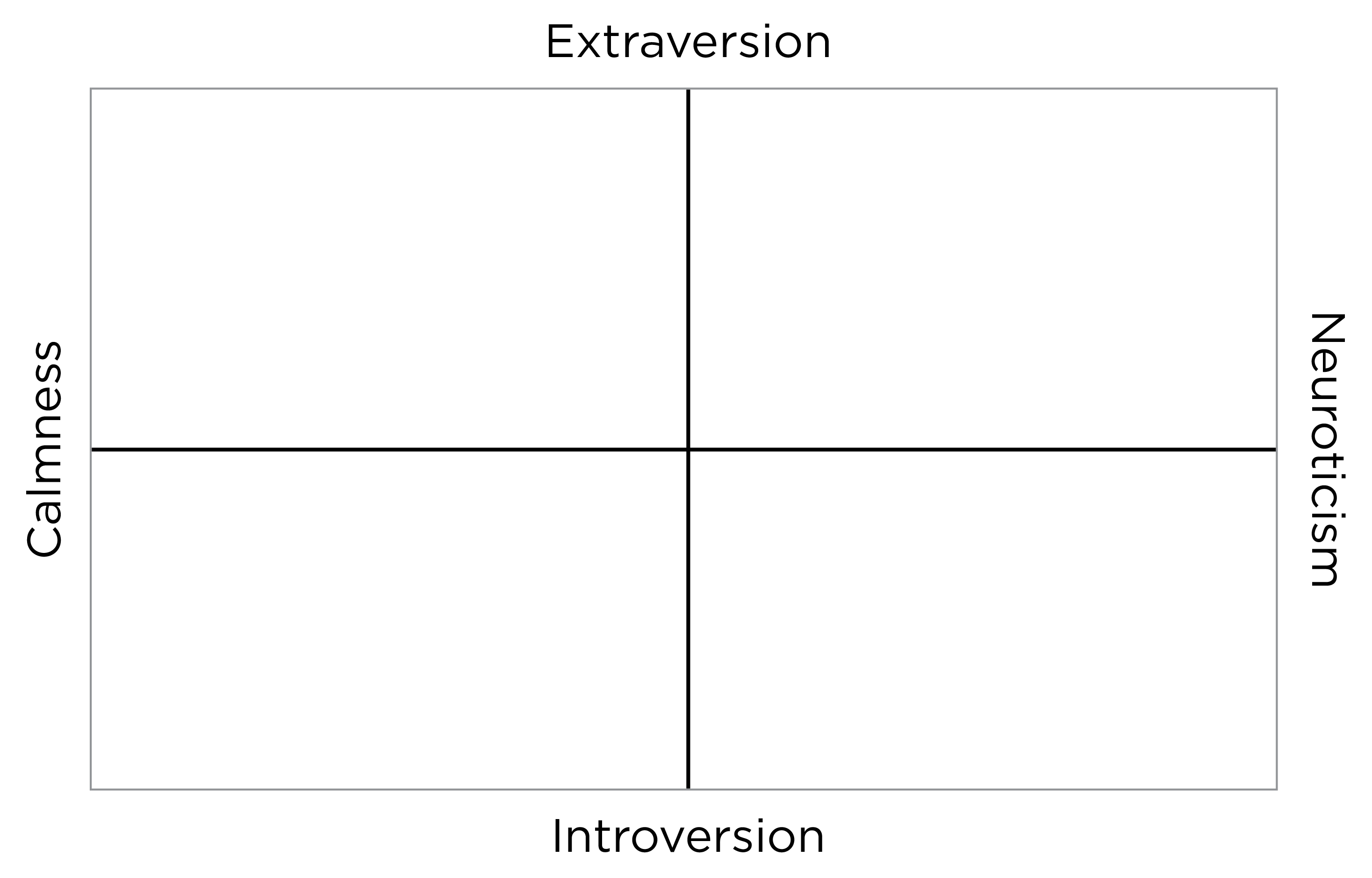
As an example of rotation based on interpretability, consider the Five-Factor Model of Personality (the Big Five), which goes by the acronym, OCEAN: Openness, Conscientiousness, Extraversion, Agreeableness, and Neuroticism. Although the five factors of personality are somewhat correlated, we can use rotation to ensure they are maximally independent. Upon rotation, extraversion and neuroticism are essentially uncorrelated, as depicted in Figure 14.25. The other pole of extraversion is intraversion and the other pole of neuroticism might be emotional stability or calmness.
Simple structure is achieved when each variable loads highly onto as few factors as possible (i.e., each item has only one significant or primary loading). Oftentimes this is not the case, so we choose our rotation method in order to decide if the factors can be correlated (an oblique rotation) or if the factors will be uncorrelated (an orthogonal rotation). If the factors are not correlated with each other, use an orthogonal rotation. The correlation between an item and a factor is a factor loading, which is simply a way to ask how much a variable is correlated with the underlying factor. However, its interpretation is more complicated if there are correlated factors!
An orthogonal rotation (e.g., varimax) can help with simplicity of interpretation because it seeks to yield simple structure without cross-loadings. Cross-loadings are instances where a variable loads onto multiple factors. My recommendation would always be to use an orthogonal rotation if you have reason to believe that finding simple structure in your data is possible; otherwise, the factors are extremely difficult to interpret—what exactly does a cross-loading even mean? However, you should always try an oblique rotation, too, to see how strongly the factors are correlated. If the factors are not correlated, an oblique rotation will resolve to yield similar results as an orthogonal rotation (and thus may be preferred over othogonal rotation given its flexibility). Examples of oblique rotations include oblimin and promax.
6. Model Selection and Interpretation
The next step of factor analysis is selecting and interpreting the model. One data matrix can lead to many different (correct) models—you must choose one based on the factor structure and theory. Use theory to interpret the model and label the factors. When interpreting others’ findings, do not rely just on the factor labels—look at the actual items to determine what they assess. What they are called matters much less than what the actual items are! This calls to mind the jingle-jangle fallacy. The jingle fallacy is the erroneous assumption that two different things are the same because they have the same label; the jangle fallacy is the erroneous assumption that two identical or near-identical things are different because they have different labels. Thus, it is important to evaluate the measures and what they actually assess, and not just to rely on labels and what they intend to assess.
The Downfall of Factor Analysis
The downfall of factor analysis is cross-validation. Cross-validating a factor structure would mean getting the same factor structure with a new sample. We want factor structures to show good replicability across samples. However, cross-validation often falls apart. The way to attempt to replicate a factor structure in an independent sample is to use CFA to set everything up and test the hypothesized factor structure in the independent sample.
What to Do with Factors
What can you do with factors once you have them? In SEM, factors have meaning. You can use them as predictors, mediators, moderators, or outcomes. And, using latent factors in SEM helps disattenuate associations for measurement error, as described in Section 5.6.3. People often want to use factors outside of SEM, but there is confusion here: When researchers find that three variables load onto Factor A, the researchers often combine those three using a sum or average—but this is not accurate. If you just add or average them, this ignores the factor loadings and the error. A mean or sum score is a measurement model that assumes that all items have the same factor loading (i.e., a loading of 1) and no error (residual of 0), which is unrealistic. Another solution is to form a linear composite by adding and weighting the variables by the factor loadings, which retains the differences in correlations (i.e., a weighted sum), but this still ignores the estimated error, so it still may not be generalizable and meaningful. At the same time, weighted sums may be less generalizable than unit-weighted composites where each variable is given equal weight (Garb & Wood, 2019; Wainer, 1976) because some variability in factor loadings likely reflects sampling error.
A comparison of various measurement models is in Table 14.1.
Missing Data Handling
The PCA default in SPSS is listwise deletion of missing data: if a participant is missing data on any variable, the subject gets excluded from the analysis, so you might end up with too few participants. Instead, use a correlation matrix with pairwise deletion for PCA with missing data. Maximum likelihood factor analysis can make use of all available data points for a participant, even if they are missing some data points. Mplus, which is often used for SEM and factor analysis, will notify you if you are removing many participants in CFA/EFA. The lavaan package (Rosseel et al., 2022) in R also notifies you if you are removing participants in CFA/SEM models.
Troubleshooting Improper Solutions
A PCA will always converge; however, a factor analysis model may not converge. If a factor analysis model does not converge, you will need to modify the model to get it to converge. Model identification is described here.
In addition, a factor analysis model may converge but be improper. For example, if the factor analysis model has a negative residual variance or correlation above 1, the model is improper. A negative residual variance is also called a Heywood case. Problematic parameters such as a negative residual variance or correlation above 1 can lead to problems with other parameters in the model. It is thus preferable to avoid or address improper solutions. A negative residual variance or correlation above 1 could be caused by a variety of things such as a misspecified model, too many factors, too few indicators per factor, or too few participants (relative to the complexity of the model). Another issue that could arise is a non-positive definite matrix. A non-positive definite matrix could also be caused by a variety of things such as multicollinearity or singularity, variables with zero variance, too many variables relative to the sample size, or too many factors.
Here are various ways you may troubleshoot improper solutions in factor analysis:
- Modify the model to be a represent a truer representation of the data-generating process
- Simplify the model
- Estimate fewer paths/parameters
- Reduce the number of factors estimated/extracted
- Reduce the number of indicators included, either by removing variables or by parceling items (Little et al., 2002, 2013)
- Increase the sample size
- Increase the number of indicators per factor
- Drop the offending item that has a negative residual variance (if theoretically justifiable because the item may be poorly performing)
- Use different starting values
- Test whether the negative residual variance is significantly different from zero; if not, can consider fixing it to zero (though this is not an ideal solution)
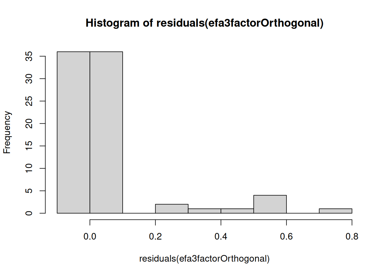
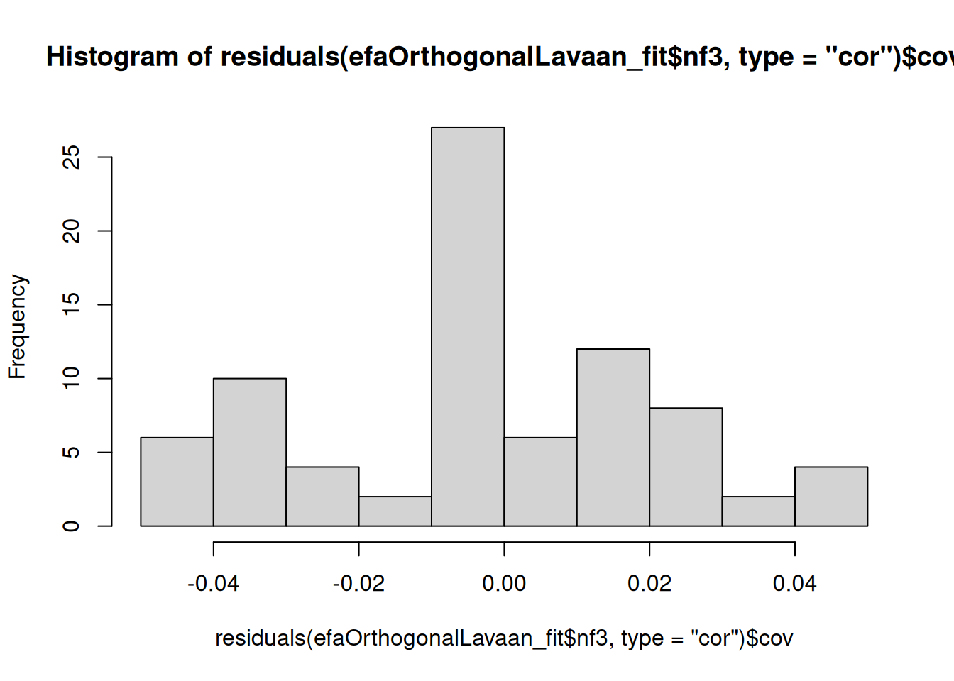
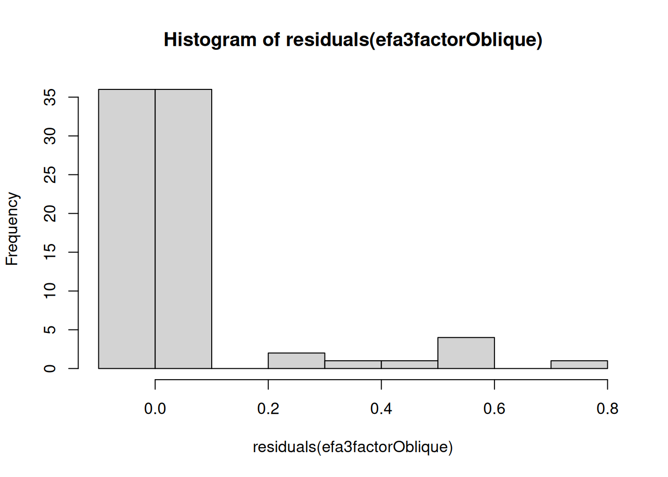
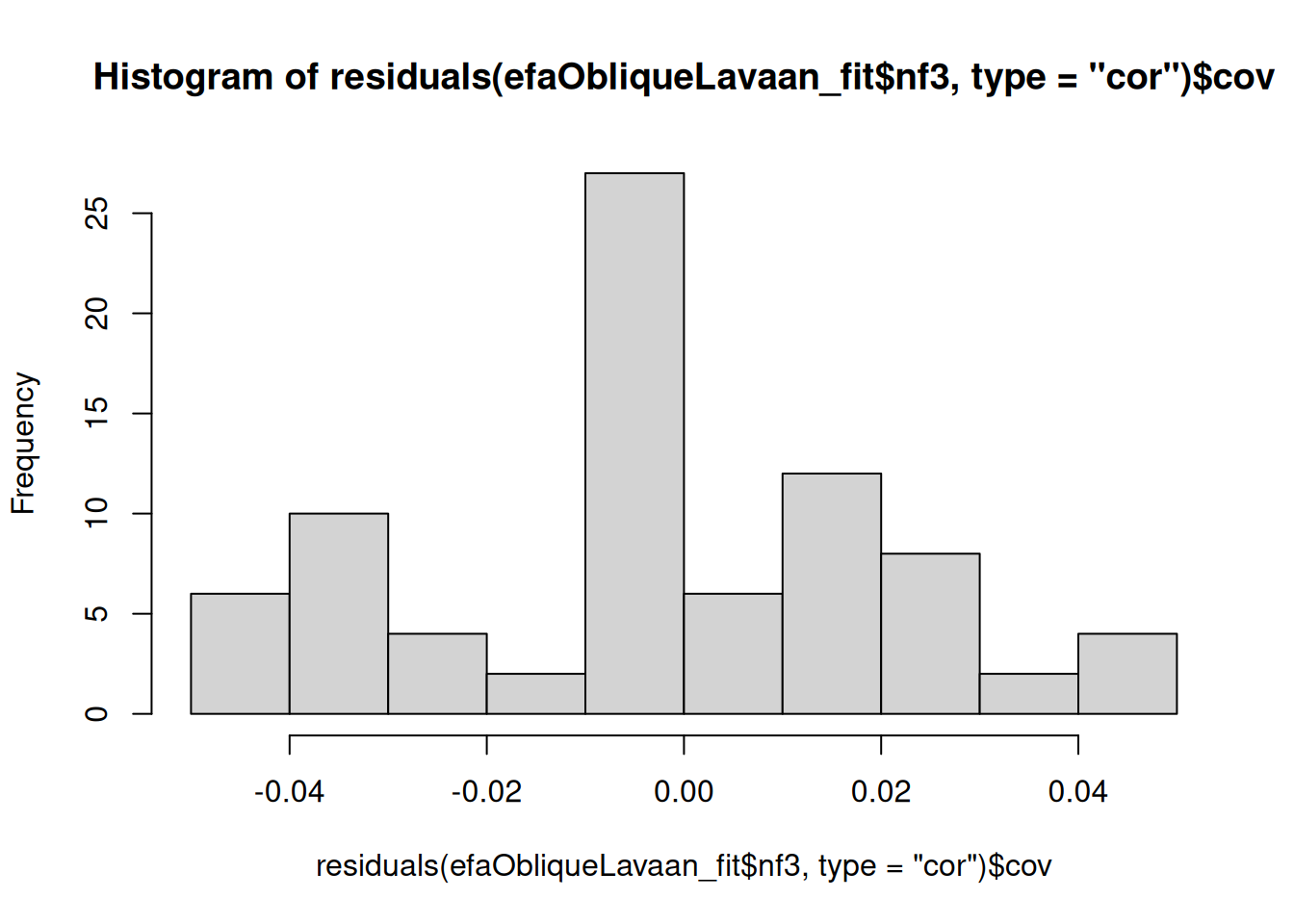
- Examine the data (e.g., using a histogram) for possible outliers or for variables with minimal variance
- Examine a correlation matrix of the data for variables that are insufficiently associated for estimating a latent factor, or for variables that are so strongly correlated to be redundant
- Use regularization with constraints so the residual variances do not become negative