I want your feedback to make the book better for you and other readers. If you find typos, errors, or places where the text may be improved, please let me know.
The best ways to provide feedback are by GitHub or hypothes.is annotations.
Adding an annotation using hypothes.is.
To add an annotation, select some text and then click the
symbol on the pop-up menu.
To see the annotations of others, click the
symbol in the upper right-hand corner of the page.
8Item Response Theory
In the chapter on reliability, we introduced classical test theory. Classical test theory is a measurement theory of how test scores relate to a construct. Classical test theory provides a way to estimate the relation between the measure (or item) and the construct. For instance, with a classical test theory approach, to estimate the relation between an item and the construct, you would compute an item–total correlation. An item–total correlation is the correlation of an item with the total score on the measure (e.g., sum score). The item–total correlation approximates the relation between an item and the construct. However, the item–total correlation is a crude estimate of the relation between an item and the construct. And there are many other ways to characterize the relation between an item and a construct. One such way is with item response theory (IRT).
8.1 Overview of IRT
Unlike classical test theory, which is a measurement theory of how test scores relate to a construct, IRT is a measurement theory that describes how an item is related to a construct. For instance, given a particular person’s level on the construct, what is their chance of answering “TRUE” on a particular item?
IRT is an approach to latent variable modeling. In IRT, we estimate a person’s construct score (i.e., level on the construct) based on their item responses. The construct is estimated as a latent factor that represents the common variance among all items as in structural equation modeling or confirmatory factor analysis. The person’s level on the construct is called theta (\(\theta\)). When dealing with performance-based tests, theta is sometimes called “ability.”
8.1.1 Item Characteristic Curve
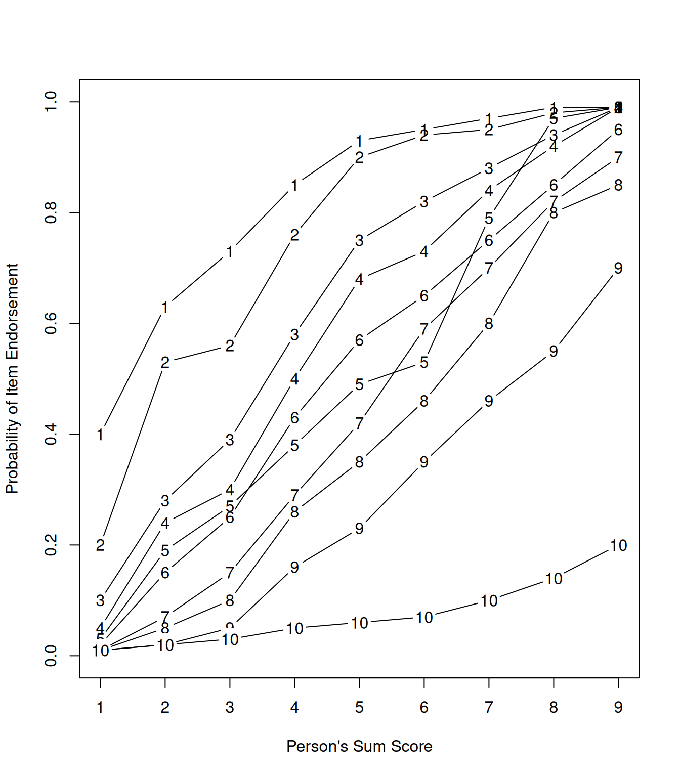
In IRT, we can plot an item characteristic curve (ICC). The ICC is a plot of the model-derived probability of a symptom being present (or a correct response) as a function of a person’s standing on a latent continuum. For instance, we can create empirical ICCs that can take any shape (see Figure 8.1).
plot(empiricalICCdata$itemSum, empiricalICCdata$item10, type ="n", xlim =c(1,9), ylim =c(0,1), xlab ="Person's Sum Score", ylab ="Probability of Item Endorsement", xaxt ="n")lines(empiricalICCdata$itemSum, empiricalICCdata$item1, type ="b", pch ="1")lines(empiricalICCdata$itemSum, empiricalICCdata$item2, type ="b", pch ="2")lines(empiricalICCdata$itemSum, empiricalICCdata$item3, type ="b", pch ="3")lines(empiricalICCdata$itemSum, empiricalICCdata$item4, type ="b", pch ="4")lines(empiricalICCdata$itemSum, empiricalICCdata$item5, type ="b", pch ="5")lines(empiricalICCdata$itemSum, empiricalICCdata$item6, type ="b", pch ="6")lines(empiricalICCdata$itemSum, empiricalICCdata$item7, type ="b", pch ="7")lines(empiricalICCdata$itemSum, empiricalICCdata$item8, type ="b", pch ="8")lines(empiricalICCdata$itemSum, empiricalICCdata$item9, type ="b", pch ="9")lines(empiricalICCdata$itemSum, empiricalICCdata$item10, type ="l")points(empiricalICCdata$itemSum, empiricalICCdata$item10, type ="p", pch =19, col ="white", cex =3)text(empiricalICCdata$itemSum, empiricalICCdata$item10, labels ="10")axis(1, at =1:9, labels =1:9)
Figure 8.1: Empirical Item Characteristic Curves of the Probability of Endorsement of a Given Item as a Function of the Person’s Sum Score.
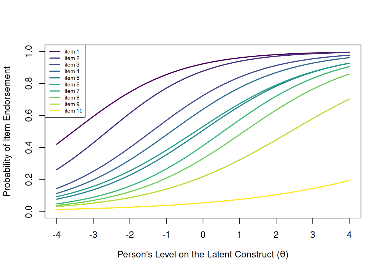
In a model-implied ICC, we fit a logistic (sigmoid) curve to each item’s probability of a symptom being present as a function of a person’s level on the latent construct. The model-implied ICCs for the same 10 items from Figure 8.1 are depicted in Figure 8.2.
Code
#https://www.statforbiology.com/nonlinearregression/usefulequations#logistic_curve; archived at https://perma.cc/8WFX-FCEQ#https://github.com/OnofriAndreaPG/aomisc/blob/1eb698b3bc5f55a718c37bfd2028b9ac73a6fbbe/R/SSL.R; archived at https://perma.cc/94CM-PSGYlibrary("viridis")#Log-Logistic Function nlsL.2 (similar to L.3 from drc package)L2.fun <-function(predictor, a, b) { x <- predictor1/(1+exp( - a* (x - b)))}L2.Init <-function(mCall, LHS, data, ...) { xy <-sortedXyData(mCall[["predictor"]], LHS, data) x <- xy[, "x"]; y <- xy[, "y"] d <-1## Linear regression on pseudo y values pseudoY <-log((d - y)/(y+0.00001)) coefs <-coef( lm(pseudoY ~ x)) k <- coefs[1]; a <-- coefs[2] b <- k/a value <-c(a, b)names(value) <- mCall[c("a", "b")] value}NLS.L2 <-selfStart(L2.fun, L2.Init, parameters =c("a", "b"))twoPLitem1 <-nls(item1 ~NLS.L2(itemSum, a, b), data = empiricalICCdata, control =list(warnOnly =TRUE))twoPLitem2 <-nls(item2 ~NLS.L2(itemSum, a, b), data = empiricalICCdata, control =list(warnOnly =TRUE))twoPLitem3 <-nls(item3 ~NLS.L2(itemSum, a, b), data = empiricalICCdata, control =list(warnOnly =TRUE))twoPLitem4 <-nls(item4 ~NLS.L2(itemSum, a, b), data = empiricalICCdata, control =list(warnOnly =TRUE))twoPLitem5 <-nls(item5 ~NLS.L2(itemSum, a, b), data = empiricalICCdata, control =list(warnOnly =TRUE))twoPLitem6 <-nls(item6 ~NLS.L2(itemSum, a, b), data = empiricalICCdata, control =list(warnOnly =TRUE))twoPLitem7 <-nls(item7 ~NLS.L2(itemSum, a, b), data = empiricalICCdata, control =list(warnOnly =TRUE))twoPLitem8 <-nls(item8 ~NLS.L2(itemSum, a, b), data = empiricalICCdata, control =list(warnOnly =TRUE))twoPLitem9 <-nls(item9 ~NLS.L2(itemSum, a, b), data = empiricalICCdata, control =list(warnOnly =TRUE))twoPLitem10 <-nls(item10 ~NLS.L2(itemSum, a, b), data = empiricalICCdata, control =list(warnOnly =TRUE))newdata <-data.frame(itemSum =seq(from =1, to =9, length.out =1000))newdata$item1 <-predict(twoPLitem1, newdata = newdata)newdata$item2 <-predict(twoPLitem2, newdata = newdata)newdata$item3 <-predict(twoPLitem3, newdata = newdata)newdata$item4 <-predict(twoPLitem4, newdata = newdata)newdata$item5 <-predict(twoPLitem5, newdata = newdata)newdata$item6 <-predict(twoPLitem6, newdata = newdata)newdata$item7 <-predict(twoPLitem7, newdata = newdata)newdata$item8 <-predict(twoPLitem8, newdata = newdata)newdata$item9 <-predict(twoPLitem9, newdata = newdata)newdata$item10 <-predict(twoPLitem10, newdata = newdata)newdata$itemTotal <-rowSums(newdata[,paste("item", 1:10, sep ="")])
Code
plot(newdata$itemSum, newdata$item1, type ="n", ylim =c(0,1), xlab =expression(paste("Person's Level on the Latent Construct (", theta, ")", sep ="")), ylab ="Probability of Item Endorsement", xaxt ="n")lines(newdata$itemSum, newdata$item1, type ="l", lwd =2, col =viridis(10)[1])lines(newdata$itemSum, newdata$item2, type ="l", lwd =2, col =viridis(10)[2])lines(newdata$itemSum, newdata$item3, type ="l", lwd =2, col =viridis(10)[3])lines(newdata$itemSum, newdata$item4, type ="l", lwd =2, col =viridis(10)[4])lines(newdata$itemSum, newdata$item5, type ="l", lwd =2, col =viridis(10)[5])lines(newdata$itemSum, newdata$item6, type ="l", lwd =2, col =viridis(10)[6])lines(newdata$itemSum, newdata$item7, type ="l", lwd =2, col =viridis(10)[7])lines(newdata$itemSum, newdata$item8, type ="l", lwd =2, col =viridis(10)[8])lines(newdata$itemSum, newdata$item9, type ="l", lwd =2, col =viridis(10)[9])lines(newdata$itemSum, newdata$item10, type ="l", lwd =2, col =viridis(10)[10])axis(1, at =seq(from =1, to =9, length.out =9), labels =c(-4:4))legend("topleft", legend =paste("item", 1:10, sep =" "), col =viridis(10), lwd =2, cex =0.6)
Figure 8.2: Item Characteristic Curves of the Probability of Endorsement of a Given Item as a Function of the Person’s Level on the Latent Construct.
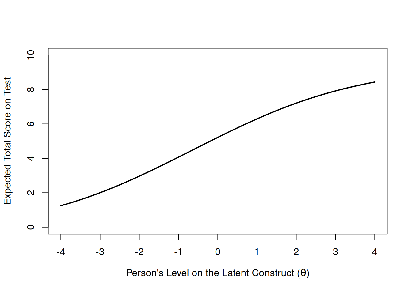
ICCs can be summed across items to get the test characteristic curve (TCC):
Code
plot(newdata$itemSum, newdata$itemTotal, type ="n", ylim =c(0,10), xlab =expression(paste("Person's Level on the Latent Construct (", theta, ")", sep ="")), ylab ="Expected Total Score on Test", xaxt ="n")lines(newdata$itemSum, newdata$itemTotal, type ="l", lwd =2)axis(1, at =seq(from =1, to =9, length.out =9), labels =c(-4:4))
Figure 8.3: Test Characteristic Curve of the Expected Total Score on the Test as a Function of the Person’s Level on the Latent Construct.
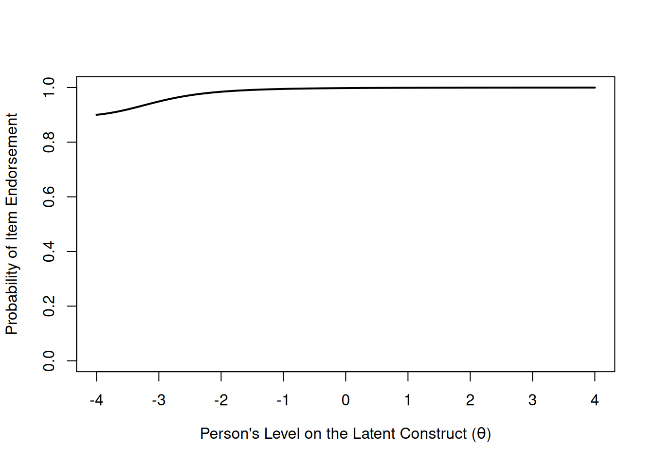
An ICC provides more information than an item–total correlation. Visually, we can see the utility of various items by looking at the items’ ICC plots. For instance, consider what might be a useless item for diagnostic purposes. For a particular item, among those with a low total score (level on the construct), 90% respond with “TRUE” to the item, whereas among everyone else, 100% respond with “TRUE” (see Figure 8.4). This item has a ceiling effect and provides only a little information about who would be considered above clinical threshold for a disorder. So, the item is not very clinically useful.
Code
library("drc")empiricalICCdata$ceilingEffect <-c(.90, .95, .98, 1, 1, 1, 1, 1, 1)empiricalICCdata$diagnosticallyUseful <-c(0, 0, 0, 0, 0, 0, .69, .70, .70)threePL_ceilingeffect <-drm(ceilingEffect ~ itemSum, data = empiricalICCdata, fct =LL.3u(), type ="continuous") #fix upper asymptote at 1threePL_diagnosticallyUseful <-drm(diagnosticallyUseful ~ itemSum, data = empiricalICCdata, fct =LL.3(), type ="continuous") #fix lower asymptote at 0newdata$ceilingEffect <-predict(threePL_ceilingeffect, newdata = newdata)newdata$diagnosticallyUseful <-predict(threePL_diagnosticallyUseful, newdata = newdata)
Code
plot(newdata$itemSum, newdata$ceilingEffect, type ="l", lwd =2, ylim =c(0,1), xlab =expression(paste("Person's Level on the Latent Construct (", theta, ")", sep ="")), ylab ="Probability of Item Endorsement", xaxt ="n")axis(1, at =seq(from =1, to =9, length.out =9), labels =c(-4:4))
Figure 8.4: Item Characteristic Curve of an Item with a Ceiling Effect That is not Diagnostically Useful.
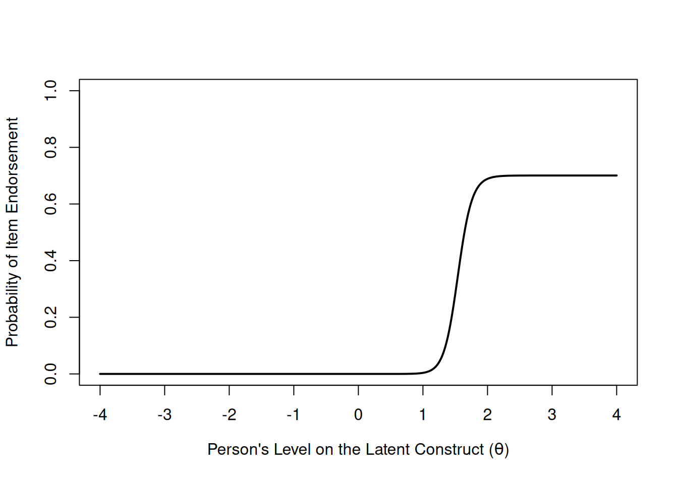
Now, consider a different item. For those with a low level on the construct, 0% respond with “TRUE”, so it has a floor effect and tells us nothing about the lower end of the construct. But for those with a higher level on the construct, 70% respond with true (see Figure 8.5). So, the item tells us something about the higher end of the distribution, and could be diagnostically useful. Thus, an ICC allows us to immediately tell the utility of items.
Code
plot(newdata$itemSum, newdata$diagnosticallyUseful, type ="l", lwd =2, ylim =c(0,1), xlab =expression(paste("Person's Level on the Latent Construct (", theta, ")", sep ="")), ylab ="Probability of Item Endorsement", xaxt ="n")axis(1, at =seq(from =1, to =9, length.out =9), labels =c(-4:4))
Figure 8.5: Item Characteristic Curve of an Item With a Floor Effect That is Diagnostically Useful.
8.1.2 Parameters
We can estimate up to four parameters in an IRT model and can glean up to four key pieces of information from an item’s ICC:
Difficulty (severity)
Discrimination
Guessing
Inattention/careless errors
8.1.2.1 Difficulty (Severity)
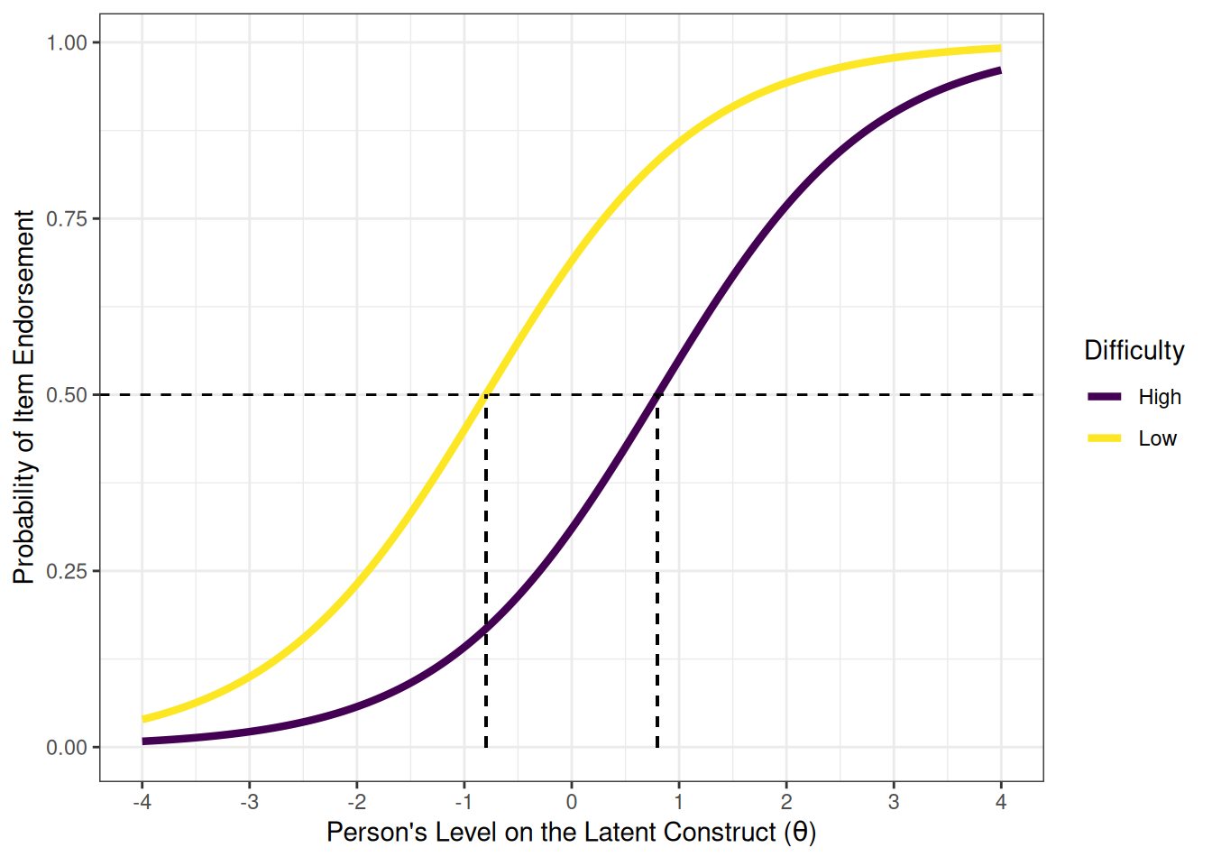
The item’s difficulty parameter is the item’s location on the latent construct. It is quantified by the intercept, i.e., the location on the x-axis of the inflection point of the ICC. In a 1- or 2-parameter model, the inflection point is where 50% of the sample endorses the item (or gets the item correct), that is, the point on the x-axis where the ICC crosses .5 probability on the y-axis (i.e., the level on the construct at which the probability of endorsing the item is equal to the probability of not endorsing the item). Item difficulty is similar to item means or intercepts in structural equation modeling or factor analysis. Some items are more useful at the higher levels of the construct, whereas other items are more useful at the lower levels of the construct. See Figure 8.6 for an example of an item with a low difficulty and an item with a high difficulty.
Code
library("tidyverse")library("psych")difficultyData <-data.frame(itemSum =1:length(-4:4))difficultyData$lowDifficulty <- psych::logistic(-4:4, d =-0.8)difficultyData$highDifficulty <- psych::logistic(-4:4, d =0.8)L1.fun <-function(predictor, b) { x <- predictor1/(1+exp( -(x - b)))}L1.Init <-function(mCall, LHS, data, ...) { xy <-sortedXyData(mCall[["predictor"]], LHS, data) x <- xy[, "x"]; y <- xy[, "y"] d <-1## Linear regression on pseudo y values pseudoY <-log((d - y)/(y+0.00001)) coefs <-coef( lm(pseudoY ~ x)) k <- coefs[1] b <- coefs[2] value <-c(b)names(value) <- mCall[c("b")] value}NLS.L1 <-selfStart(L1.fun, L1.Init, parameters =c("b"))onePL_lowDifficulty <-nls(lowDifficulty ~NLS.L1(itemSum, b), data = difficultyData, control =list(warnOnly =TRUE))onePL_highDifficulty <-nls(highDifficulty ~NLS.L1(itemSum, b), data = difficultyData, control =list(warnOnly =TRUE))newdata$lowDifficulty <-predict(onePL_lowDifficulty, newdata = newdata)newdata$highDifficulty <-predict(onePL_highDifficulty, newdata = newdata)newdata$theta <-seq(from =-4, to =4, length.out =1000)midpoint_lowDifficulty <- newdata$theta[which.min(abs(newdata$lowDifficulty -0.5))]midpoint_highDifficulty <- newdata$theta[which.min(abs(newdata$highDifficulty -0.5))]difficulty_long <-pivot_longer(newdata, cols = lowDifficulty:highDifficulty) %>%rename(item = name)difficulty_long$Difficulty <-NAdifficulty_long$Difficulty[which(difficulty_long$item =="lowDifficulty")] <-"Low"difficulty_long$Difficulty[which(difficulty_long$item =="highDifficulty")] <-"High"
Code
ggplot(difficulty_long, aes(theta, value, group = Difficulty, color = Difficulty)) +geom_line(linewidth =1.5) +scale_color_viridis_d() +geom_hline(yintercept =0.5, linetype ="dashed") +geom_segment(aes(x = midpoint_lowDifficulty, xend = midpoint_lowDifficulty, y =0, yend =0.5), linewidth =0.5, col ="black", linetype ="dashed") +geom_segment(aes(x = midpoint_highDifficulty, xend = midpoint_highDifficulty, y =0, yend =0.5), linewidth =0.5, col ="black", linetype ="dashed") +scale_x_continuous(name =expression(paste("Person's Level on the Latent Construct (", theta, ")", sep ="")), breaks =-4:4) +scale_y_continuous(name ="Probability of Item Endorsement") +theme_bw()
Figure 8.6: Item Characteristic Curves of an Item With Low Difficulty Versus High Difficulty. The dashed horizontal line indicates a probability of item endorsement of .50. The dashed vertical line is the item difficulty, i.e., the person’s level on the construct (the location on the x-axis) at the inflection point of the item characteristic curve. In a two-parameter logistic model, the inflection point corresponds to the probability of item endorsement is 50%. Thus, in a two-parameter logistic model, the difficulty of an item is the person’s level on the construct where the probability of endorsing the item is 50%.
When dealing with a measure of clinical symptoms (e.g., depression), the difficulty parameter is sometimes called severity, because symptoms that are endorsed less frequently tend to be more severe (e.g., suicidal behavior; Krueger et al., 2004). One way of thinking about the severity parameter of an item is: “How severe does your psychopathology have to be for half of people to endorse the symptom?”
When dealing with a measure of performance, aptitude, or intelligence, the parameter would be more likely to be called difficulty: “How high does your ability have to be for half of people to pass the item?” An item with a low difficulty would be considered easy, because even people with a low ability tend to pass the item. An item with a high difficulty would be considered difficult, because only people with a high ability tend to pass the item.
8.1.2.2 Discrimination
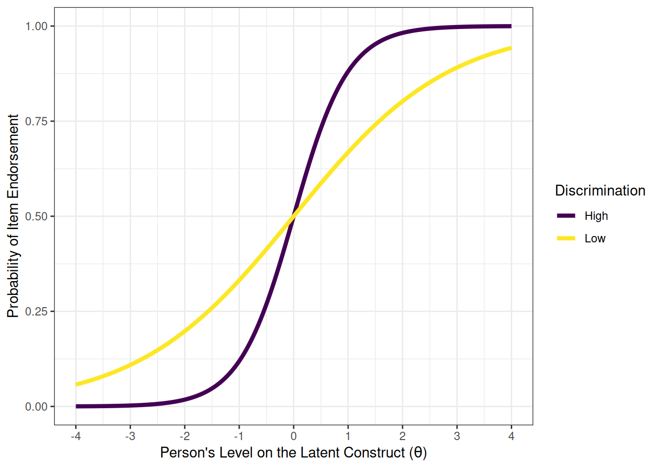
The item’s discrimination parameter is how well the item can distinguish between those who were higher versus lower on the construct, that is, how strongly the item is correlated with the construct (i.e., the latent factor). It is similar to the factor loading in structural equation modeling or factor analysis. It is quantified by the slope of the ICC, i.e., the steepness of the line at its steepest point. The slope reflects the inverse of how much range of construct levels it would take to flip 50/50 whether a person is likely to pass or fail an item.
Some items have ICCs that go up fast (have a steep slope). These items provide a fine distinction between people with lower versus higher levels on the construct and therefore have high discrimination. Some items go up gradually (less steep slope), so it provides less precision and information, and has a low discrimination. See Figure 8.7 for an example of an item with a low discrimination and an item with a high discrimination.
Code
discriminationData <-data.frame(itemSum =1:length(-4:4))discriminationData$lowDiscrimination <- psych::logistic(-4:4, d =0, a =0.7)discriminationData$highDiscrimination <- psych::logistic(-4:4, d =0, a =2)twoPL_lowDiscrimination <-nls(lowDiscrimination ~NLS.L2(itemSum, a, b), data = discriminationData, control =list(warnOnly =TRUE))twoPL_highDiscrimination <-nls(highDiscrimination ~NLS.L2(itemSum, a, b), data = discriminationData, control =list(warnOnly =TRUE))newdata$lowDiscrimination <-predict(twoPL_lowDiscrimination, newdata = newdata)newdata$highDiscrimination <-predict(twoPL_highDiscrimination, newdata = newdata)newdata$theta <-seq(from =-4, to =4, length.out =1000)discrimination_long <-pivot_longer(newdata, cols = lowDiscrimination:highDiscrimination) %>%rename(item = name)discrimination_long$Discrimination <-NAdiscrimination_long$Discrimination[which(discrimination_long$item =="lowDiscrimination")] <-"Low"discrimination_long$Discrimination[which(discrimination_long$item =="highDiscrimination")] <-"High"
Code
ggplot(discrimination_long, aes(theta, value, group = Discrimination, color = Discrimination)) +geom_line(linewidth =1.5) +scale_color_viridis_d() +scale_x_continuous(name =expression(paste("Person's Level on the Latent Construct (", theta, ")", sep ="")), breaks =-4:4) +scale_y_continuous(name ="Probability of Item Endorsement") +theme_bw()
Figure 8.7: Item Characteristic Curves of an Item With Low Discrimination Versus High Discrimination. The discrimination of an item is the slope of the line at its inflection point.
8.1.2.3 Guessing
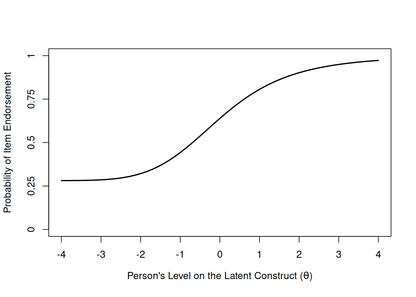
The item’s guessing parameter is reflected by the lower asymptote of the ICC. If the item has a lower asymptote above zero, it suggests that the probability of getting the item correct (or endorsing the item) never reaches zero, for any level of the construct. On an educational test, this could correspond to the person’s likelihood of being able to answer the item correctly by chance just by guessing. For example, for a 4-option multiple choice test, a respondent would be expected to get a given item correct 25% of the time just by guessing. See Figure 8.8 for an example of an item from a true/false exam and Figure 8.9 for an example of an item from a 4-option multiple choice exam.
Code
empiricalICCdata$guessingTF <- psych::logistic(-4:4, c =0.5)empiricalICCdata$guessingMC <- psych::logistic(-4:4, c =0.25)threePL_guessingTF <-drm(guessingTF ~ itemSum, data = empiricalICCdata, fct =LL.3u(), type ="continuous") #fix upper asymptote at 1threePL_guessingMC <-drm(guessingMC ~ itemSum, data = empiricalICCdata, fct =LL.3u(), type ="continuous") #fix upper asymptote at 1newdata$guessingTF <-predict(threePL_guessingTF, newdata = newdata)newdata$guessingMC <-predict(threePL_guessingMC, newdata = newdata)
Code
plot(newdata$itemSum, newdata$guessingTF, type ="l", lwd =2, ylim =c(0,1), xlab =expression(paste("Person's Level on the Latent Construct (", theta, ")", sep ="")), ylab ="Probability of Item Endorsement", xaxt ="n", yaxt ="n")axis(1, at =seq(from =1, to =9, length.out =9), labels =c(-4:4))axis(2, at =c(0, .25, .5, .75, 1), labels =c(0, .25, .5, .75, 1))
Figure 8.8: Item Characteristic Curve of an Item from a True/False Exam, There Test Takers Get the Item Correct at Least 50% of the Time.
Code
plot(newdata$itemSum, newdata$guessingMC, type ="l", lwd =2, ylim =c(0,1), xlab =expression(paste("Person's Level on the Latent Construct (", theta, ")", sep ="")), ylab ="Probability of Item Endorsement", xaxt ="n", yaxt ="n")axis(1, at =seq(from =1, to =9, length.out =9), labels =c(-4:4))axis(2, at =c(0, .25, .5, .75, 1), labels =c(0, .25, .5, .75, 1))
Figure 8.9: Item Characteristic Curve of an Item From a 4-Option Multiple Choice Exam, Where Test Takers Get the Item Correct at Least 25% of the Time.
8.1.2.4 Inattention/Careless Errors
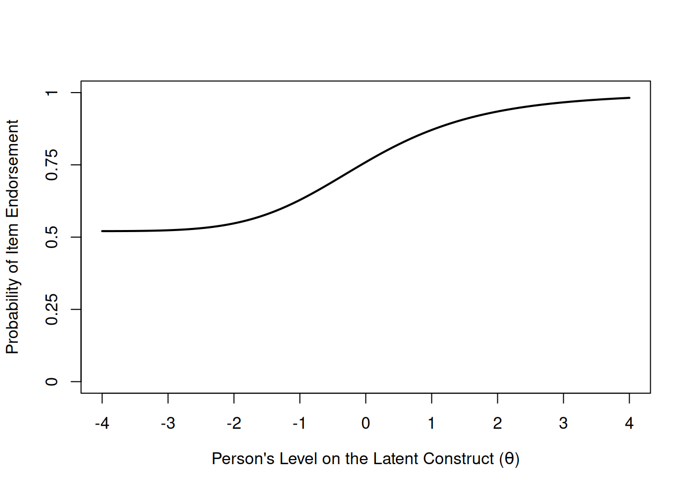
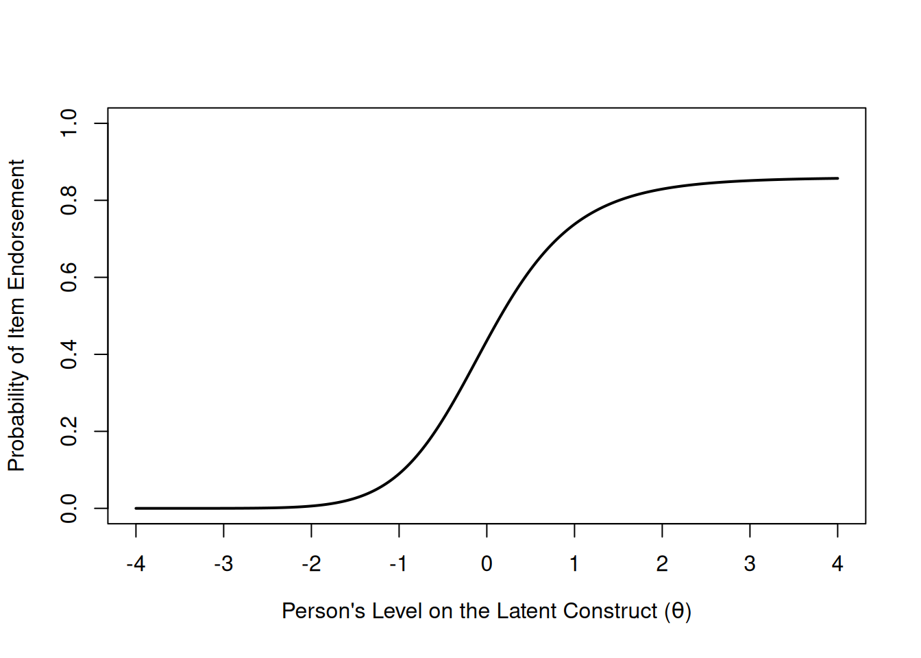
The item’s inattention (or careless error) parameter is the reflected by the upper asymptote of the ICC. If the item has an upper asymptote below one, it suggests that the probability of getting the item correct (or endorsing the item) never reaches one, for any level on the construct. See Figure 8.10 for an example of an item whose probability of endorsement (or getting it correct) exceeds .85.
Code
empiricalICCdata$inattention <- psych::logistic(-4:4, z =0.85, a =2)threePL_inattention <-drm(inattention ~ itemSum, data = empiricalICCdata, fct =LL.3(), type ="continuous") #fix lower asymptote at 0newdata$inattention <-predict(threePL_inattention, newdata = newdata)
Code
plot(newdata$itemSum, newdata$inattention, type ="l", lwd =2, ylim =c(0,1), xlab =expression(paste("Person's Level on the Latent Construct (", theta, ")", sep ="")), ylab ="Probability of Item Endorsement", xaxt ="n")axis(1, at =seq(from =1, to =9, length.out =9), labels =c(-4:4))
Figure 8.10: Item Characteristic Curve of an Item Where the Probability of Getting an Item Correct Never Exceeds .85.
8.1.3 Models
IRT models can be fit that estimate one or more of these four item parameters.
8.1.3.1 1-Parameter and Rasch models
A Rasch model estimates the item difficulty parameter and holds everything else fixed across items. It fixes the item discrimination to be one for each item. In the Rasch model, the probability that a person \(j\) with a level on the construct of \(\theta\) gets a score of one (instead of zero) on item \(i\), based on the difficulty (\(b\)) of the item, is estimated using Equation 8.1:
The petersenlab package (Petersen, 2025) contains the fourPL() function that estimates the probability of item endorsement as function of the item characteristics from the Rasch model and the person’s level on the construct (theta). To estimate the probability of endorsement from the Rasch model, specify \(b\) and \(\theta\), while keeping the defaults for the other parameters.
fourPL <-function(a =1, b, c =0, d =1, theta){ c + (d - c) * (exp(a * (theta - b))) / (1+exp(a * (theta - b)))}
Code
fourPL(b, theta)
Code
fourPL(b =1, theta =0)
[1] 0.2689414
A one-parameter logistic (1-PL) IRT model, similar to a Rasch model, estimates the item difficulty parameter, and holds everything else fixed across items (see Figure 8.11). The one-parameter logistic model holds the item discrimination fixed across items, but does not fix it to one, unlike the Rasch model.
In the one-parameter logistic model, the probability that a person \(j\) with a level on the construct of \(\theta\) gets a score of one (instead of zero) on item \(i\), based on the difficulty (\(b\)) of the item and the items’ (fixed) discrimination (\(a\)), is estimated using Equation 8.2:
The petersenlab package (Petersen, 2025) contains the fourPL() function that estimates the probability of item endorsement as function of the item characteristics from the one-parameter logistic model and the person’s level on the construct (theta). To estimate the probability of endorsement from the one-parameter logistic model, specify \(a\), \(b\), and \(\theta\), while keeping the defaults for the other parameters.
Code
fourPL(a, b, theta)
Rasch and one-parameter logistic models are common and are the easiest to fit. However, they make fairly strict assumptions. They assume that items have the same discrimination.
plot(empiricalICCdata_noCrossing$itemSum, empiricalICCdata_noCrossing$item10, type ="n", xlim =c(1,9), ylim =c(0,1), xlab ="Person's Sum Score", ylab ="Probability of Item Endorsement", xaxt ="n")lines(empiricalICCdata_noCrossing$itemSum, empiricalICCdata_noCrossing$item1, type ="b", pch ="1")lines(empiricalICCdata_noCrossing$itemSum, empiricalICCdata_noCrossing$item2, type ="b", pch ="2")lines(empiricalICCdata_noCrossing$itemSum, empiricalICCdata_noCrossing$item3, type ="b", pch ="3")lines(empiricalICCdata_noCrossing$itemSum, empiricalICCdata_noCrossing$item4, type ="b", pch ="4")lines(empiricalICCdata_noCrossing$itemSum, empiricalICCdata_noCrossing$item5, type ="b", pch ="5")lines(empiricalICCdata_noCrossing$itemSum, empiricalICCdata_noCrossing$item6, type ="b", pch ="6")lines(empiricalICCdata_noCrossing$itemSum, empiricalICCdata_noCrossing$item7, type ="b", pch ="7")lines(empiricalICCdata_noCrossing$itemSum, empiricalICCdata_noCrossing$item8, type ="b", pch ="8")lines(empiricalICCdata_noCrossing$itemSum, empiricalICCdata_noCrossing$item9, type ="b", pch ="9")lines(empiricalICCdata_noCrossing$itemSum, empiricalICCdata_noCrossing$item10, type ="l")points(empiricalICCdata_noCrossing$itemSum, empiricalICCdata_noCrossing$item10, type ="p", pch =19, col ="white", cex =3)text(empiricalICCdata_noCrossing$itemSum, empiricalICCdata_noCrossing$item10, labels ="10")axis(1, at =1:9, labels =1:9)
Figure 8.12: Empirical Item Characteristic Curves of the Probability of Endorsement of a Given Item as a Function of the Person’s Sum Score. The empirical item characteristic curves of these items do not cross each other.
8.1.3.2 2-Parameter
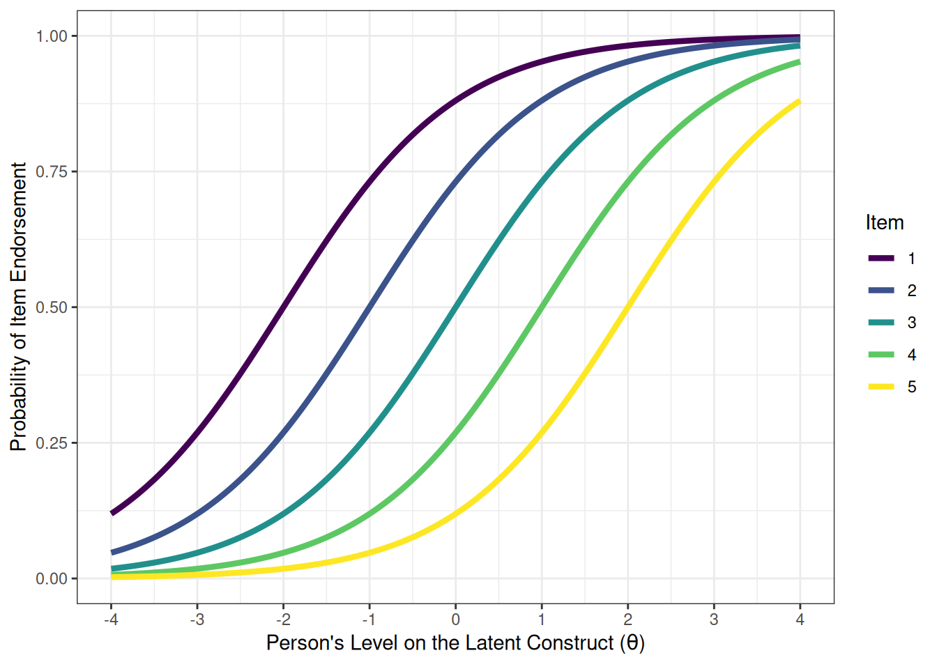
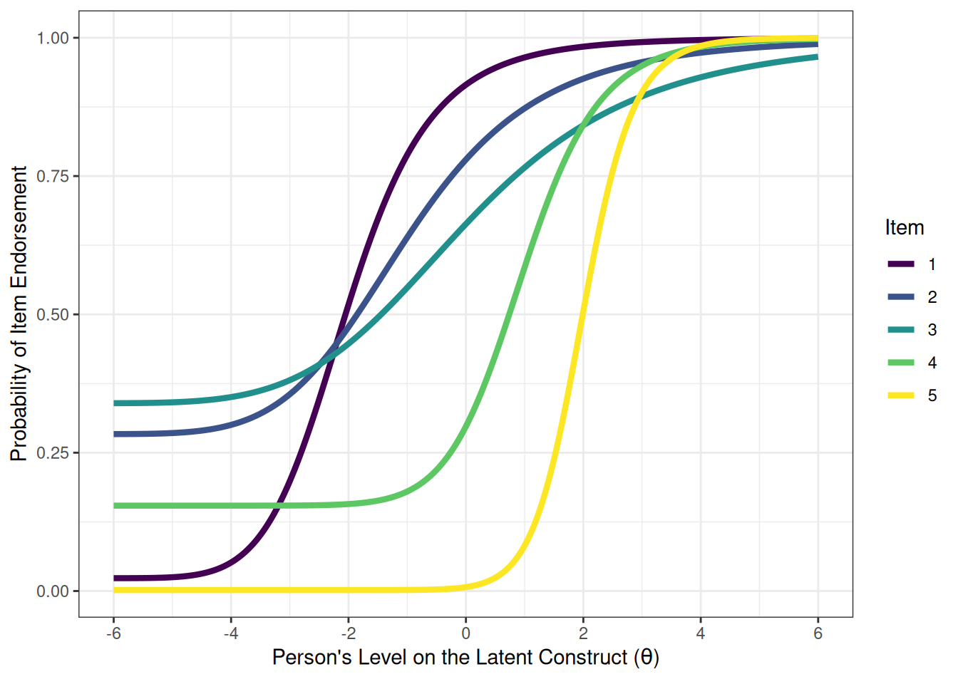
A two-parameter logistic (2-PL) IRT model estimates item difficulty and discrimination, and it holds the asymptotes fixed across items (see Figure 8.13). Two-parameter logistic models are also common.
In the two-parameter logistic model, the probability that a person \(j\) with a level on the construct of \(\theta\) gets a score of one (instead of zero) on item \(i\), based on the difficulty (\(b\)) and discrimination (\(a\)) of the item, is estimated using Equation 8.3:
The petersenlab package (Petersen, 2025) contains the fourPL() function that estimates the probability of item endorsement as function of the item characteristics from the two-parameter logistic model and the person’s level on the construct (theta). To estimate the probability of endorsement from the two-parameter logistic model, specify \(a\), \(b\), and \(\theta\), while keeping the defaults for the other parameters.
Code
fourPL(a, b, theta)
Code
fourPL(a =0.6, b =0, theta =-1)
[1] 0.3543437
Code
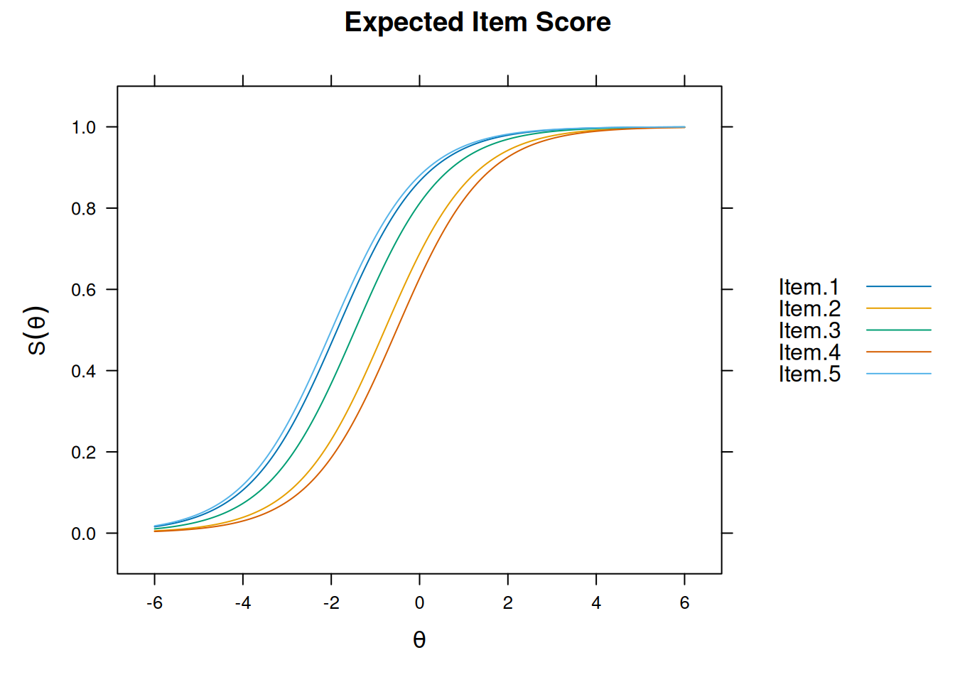
twoPLitems <-data.frame(theta =-6:6,item1 =fourPL(a =1.3, b =-2, theta =-6:6),item2 =fourPL(a =0.8, b =-1, theta =-6:6),item3 =fourPL(a =0.6, b =0, theta =-6:6),item4 =fourPL(a =1.5, b =1, theta =-6:6),item5 =fourPL(a =2.3, b =2, theta =-6:6))twoPL_item1 <-nls(item1 ~NLS.L2(theta, a, b), data = twoPLitems, control =list(warnOnly =TRUE))twoPL_item2 <-nls(item2 ~NLS.L2(theta, a, b), data = twoPLitems, control =list(warnOnly =TRUE))twoPL_item3 <-nls(item3 ~NLS.L2(theta, a, b), data = twoPLitems, control =list(warnOnly =TRUE))twoPL_item4 <-nls(item4 ~NLS.L2(theta, a, b), data = twoPLitems, control =list(warnOnly =TRUE))twoPL_item5 <-nls(item5 ~NLS.L2(theta, a, b), data = twoPLitems, control =list(warnOnly =TRUE))twoPLitems_newdata <-data.frame(theta =seq(from =-6, to =6, length.out =1000))twoPLitems_newdata$item1 <-predict(twoPL_item1, newdata = twoPLitems_newdata)twoPLitems_newdata$item2 <-predict(twoPL_item2, newdata = twoPLitems_newdata)twoPLitems_newdata$item3 <-predict(twoPL_item3, newdata = twoPLitems_newdata)twoPLitems_newdata$item4 <-predict(twoPL_item4, newdata = twoPLitems_newdata)twoPLitems_newdata$item5 <-predict(twoPL_item5, newdata = twoPLitems_newdata)twoPLitems_long <-pivot_longer(twoPLitems_newdata, cols = item1:item5) %>%rename(item = name)twoPLitems_long$Item <-NAtwoPLitems_long$Item[which(twoPLitems_long$item =="item1")] <-1twoPLitems_long$Item[which(twoPLitems_long$item =="item2")] <-2twoPLitems_long$Item[which(twoPLitems_long$item =="item3")] <-3twoPLitems_long$Item[which(twoPLitems_long$item =="item4")] <-4twoPLitems_long$Item[which(twoPLitems_long$item =="item5")] <-5
Code
ggplot(twoPLitems_long, aes(theta, value, group =factor(Item), color =factor(Item))) +geom_line(linewidth =1.5) +labs(color ="Item") +scale_color_viridis_d() +scale_x_continuous(name =expression(paste("Person's Level on the Latent Construct (", theta, ")", sep ="")), breaks =seq(from =-6, to =6, by =2), limits =c(-6,6)) +scale_y_continuous(name ="Probability of Item Endorsement") +theme_bw()
Figure 8.13: Two-Parameter Logistic Model in Item Response Theory.
8.1.3.3 3-Parameter
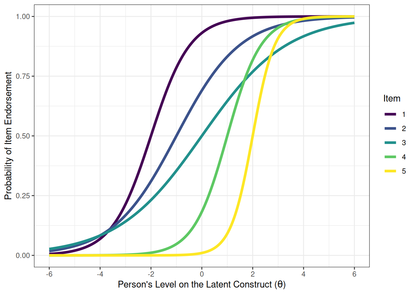
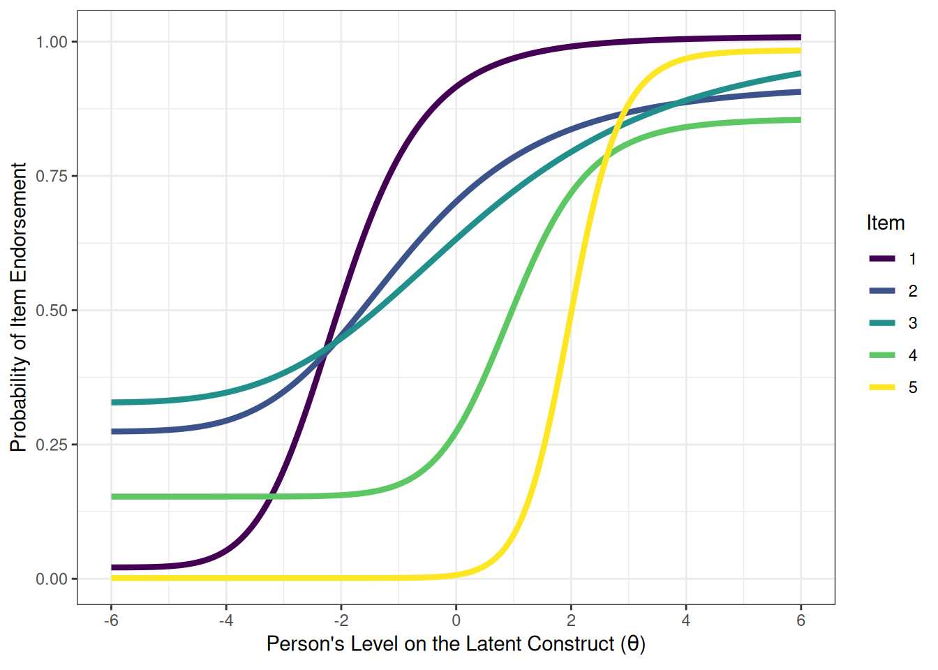
A three-parameter logistic (3-PL) IRT model estimates item difficulty, discrimination, and guessing (lower asymptote), and it holds the upper asymptote fixed across items (see Figure 8.14). This model would provide information about where an item drops out. Three-parameter logistic models are less common to estimate because it adds considerable computational complexity and requires a large sample size, and the guessing parameter is often not as important as difficulty and discrimination. Nevertheless, 3-parameter logistic models are sometimes estimated in the education literature to account for getting items correct by random guessing.
In the three-parameter logistic model, the probability that a person \(j\) with a level on the construct of \(\theta\) gets a score of one (instead of zero) on item \(i\), based on the difficulty (\(b\)), discrimination (\(a\)), and guessing parameter (\(c\)) of the item, is estimated using Equation 8.4:
The petersenlab package (Petersen, 2025) contains the fourPL() function that estimates the probability of item endorsement as function of the item characteristics from the three-parameter logistic model and the person’s level on the construct (theta). To estimate the probability of endorsement from the three-parameter logistic model, specify \(a\), \(b\), \(c\), and \(\theta\), while keeping the defaults for the other parameters.
Code
fourPL(a, b, c, theta)
Code
fourPL(a =0.8, b =-1, c = .25, theta =-1)
[1] 0.625
Code
threePLitems <-data.frame(theta =1:13,item1 =fourPL(a =1.3, b =-2, c =0, theta =-6:6),item2 =fourPL(a =0.8, b =-1, c = .25, theta =-6:6),item3 =fourPL(a =0.6, b =0, c = .3, theta =-6:6),item4 =fourPL(a =1.5, b =1, c = .15, theta =-6:6),item5 =fourPL(a =2.3, b =2, c =0, theta =-6:6))threePL_item1 <-drm(item1 ~ theta, data = threePLitems, fct =LL.3u(), type ="continuous")threePL_item2 <-drm(item2 ~ theta, data = threePLitems, fct =LL.3u(), type ="continuous")threePL_item3 <-drm(item3 ~ theta, data = threePLitems, fct =LL.3u(), type ="continuous")threePL_item4 <-drm(item4 ~ theta, data = threePLitems, fct =LL.3u(), type ="continuous")threePL_item5 <-drm(item5 ~ theta, data = threePLitems, fct =LL.3u(), type ="continuous")threePLitems_newdata <-data.frame(theta =seq(from =1, to =13, length.out =1000))threePLitems_newdata$item1 <-predict(threePL_item1, newdata = threePLitems_newdata)threePLitems_newdata$item2 <-predict(threePL_item2, newdata = threePLitems_newdata)threePLitems_newdata$item3 <-predict(threePL_item3, newdata = threePLitems_newdata)threePLitems_newdata$item4 <-predict(threePL_item4, newdata = threePLitems_newdata)threePLitems_newdata$item5 <-predict(threePL_item5, newdata = threePLitems_newdata)threePLitems_newdata$theta <-seq(from =-6, to =6, length.out =1000)threePLitems_long <-pivot_longer(threePLitems_newdata, cols = item1:item5) %>%rename(item = name)threePLitems_long$Item <-NAthreePLitems_long$Item[which(threePLitems_long$item =="item1")] <-1threePLitems_long$Item[which(threePLitems_long$item =="item2")] <-2threePLitems_long$Item[which(threePLitems_long$item =="item3")] <-3threePLitems_long$Item[which(threePLitems_long$item =="item4")] <-4threePLitems_long$Item[which(threePLitems_long$item =="item5")] <-5
Code
ggplot(threePLitems_long, aes(theta, value, group =factor(Item), color =factor(Item))) +geom_line(linewidth =1.5) +labs(color ="Item") +scale_color_viridis_d() +scale_x_continuous(name =expression(paste("Person's Level on the Latent Construct (", theta, ")", sep ="")), breaks =seq(from =-6, to =6, by =2), limits =c(-6,6)) +scale_y_continuous(name ="Probability of Item Endorsement") +theme_bw()
Figure 8.14: Three-Parameter Logistic Model in Item Response Theory.
In the four-parameter logistic model, the probability that a person \(j\) with a level on the construct of \(\theta\) gets a score of one (instead of zero) on item \(i\), based on the difficulty (\(b\)), discrimination (\(a\)), guessing parameter (\(c\)), and careless error parameter (\(d\)) of the item, is estimated using Equation 8.5:
The petersenlab package (Petersen, 2025) contains the fourPL() function that estimates the probability of item endorsement as function of the item characteristics from the four-parameter logistic model and the person’s level on the construct (theta). To estimate the probability of endorsement from the four-parameter logistic model, specify \(a\), \(b\), \(c\), \(d\), and \(\theta\).
Code
fourPL(a, b, c, d, theta)
Code
fourPL(a =1.5, b =1, c = .15, d =0.85, theta =3)
[1] 0.8168019
Code
fourPLitems <-data.frame(theta =1:13,item1 =fourPL(a =1.3, b =-2, c =0, d =1, theta =-6:6),item2 =fourPL(a =0.8, b =-1, c = .25, d =0.9, theta =-6:6),item3 =fourPL(a =0.6, b =0, c = .3, d =0.95, theta =-6:6),item4 =fourPL(a =1.5, b =1, c = .15, d =0.85, theta =-6:6),item5 =fourPL(a =2.3, b =2, c =0, d =0.98, theta =-6:6))fourPL_item1 <-drm(item1 ~ theta, data = fourPLitems, fct =LL.4(), type ="continuous")fourPL_item2 <-drm(item2 ~ theta, data = fourPLitems, fct =LL.4(), type ="continuous")fourPL_item3 <-drm(item3 ~ theta, data = fourPLitems, fct =LL.4(), type ="continuous")fourPL_item4 <-drm(item4 ~ theta, data = fourPLitems, fct =LL.4(), type ="continuous")fourPL_item5 <-drm(item5 ~ theta, data = fourPLitems, fct =LL.4(), type ="continuous")fourPLitems_newdata <-data.frame(theta =seq(from =1, to =13, length.out =1000))fourPLitems_newdata$item1 <-predict(fourPL_item1, newdata = fourPLitems_newdata)fourPLitems_newdata$item2 <-predict(fourPL_item2, newdata = fourPLitems_newdata)fourPLitems_newdata$item3 <-predict(fourPL_item3, newdata = fourPLitems_newdata)fourPLitems_newdata$item4 <-predict(fourPL_item4, newdata = fourPLitems_newdata)fourPLitems_newdata$item5 <-predict(fourPL_item5, newdata = fourPLitems_newdata)fourPLitems_newdata$theta <-seq(from =-6, to =6, length.out =1000)fourPLitems_long <-pivot_longer(fourPLitems_newdata, cols = item1:item5) %>%rename(item = name)fourPLitems_long$Item <-NAfourPLitems_long$Item[which(fourPLitems_long$item =="item1")] <-1fourPLitems_long$Item[which(fourPLitems_long$item =="item2")] <-2fourPLitems_long$Item[which(fourPLitems_long$item =="item3")] <-3fourPLitems_long$Item[which(fourPLitems_long$item =="item4")] <-4fourPLitems_long$Item[which(fourPLitems_long$item =="item5")] <-5
Code
ggplot(fourPLitems_long, aes(theta, value, group =factor(Item), color =factor(Item))) +geom_line(linewidth =1.5) +labs(color ="Item") +scale_color_viridis_d() +scale_x_continuous(name =expression(paste("Person's Level on the Latent Construct (", theta, ")", sep ="")), breaks =seq(from =-6, to =6, by =2), limits =c(-6,6)) +scale_y_continuous(name ="Probability of Item Endorsement") +theme_bw()
Figure 8.15: Four-Parameter Logistic Model in Item Response Theory.
8.1.3.5 Graded Response Model
Graded response models and generalized partial credit models can be estimated with one, two, three, or four parameters. However, they use polytomous data (not dichotomous data), as described in the section below.
In the model, \(a_i\) an item-specific discrimination parameter, \(b_{ic}\) is an item- and category-specific difficulty parameter, and \(θ_n\) is an estimate of a person’s standing on the latent variable. In the model, \(i\) represents unique items, \(c\) represents different categories that are rated, and \(j\) represents participants.
8.1.4 Type of Data
IRT models are most commonly estimated with binary or dichotomous data. For example, the measures have questions or items that can be considered collapsed into two groups (e.g., true/false, correct/incorrect, endorsed/not endorsed). IRT models can also be estimated with polytomous data (e.g., likert scale), which adds computational complexity. IRT models with polytomous data can be fit with a graded response model or generalized partial credit model.
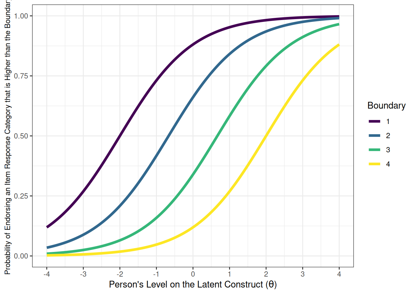
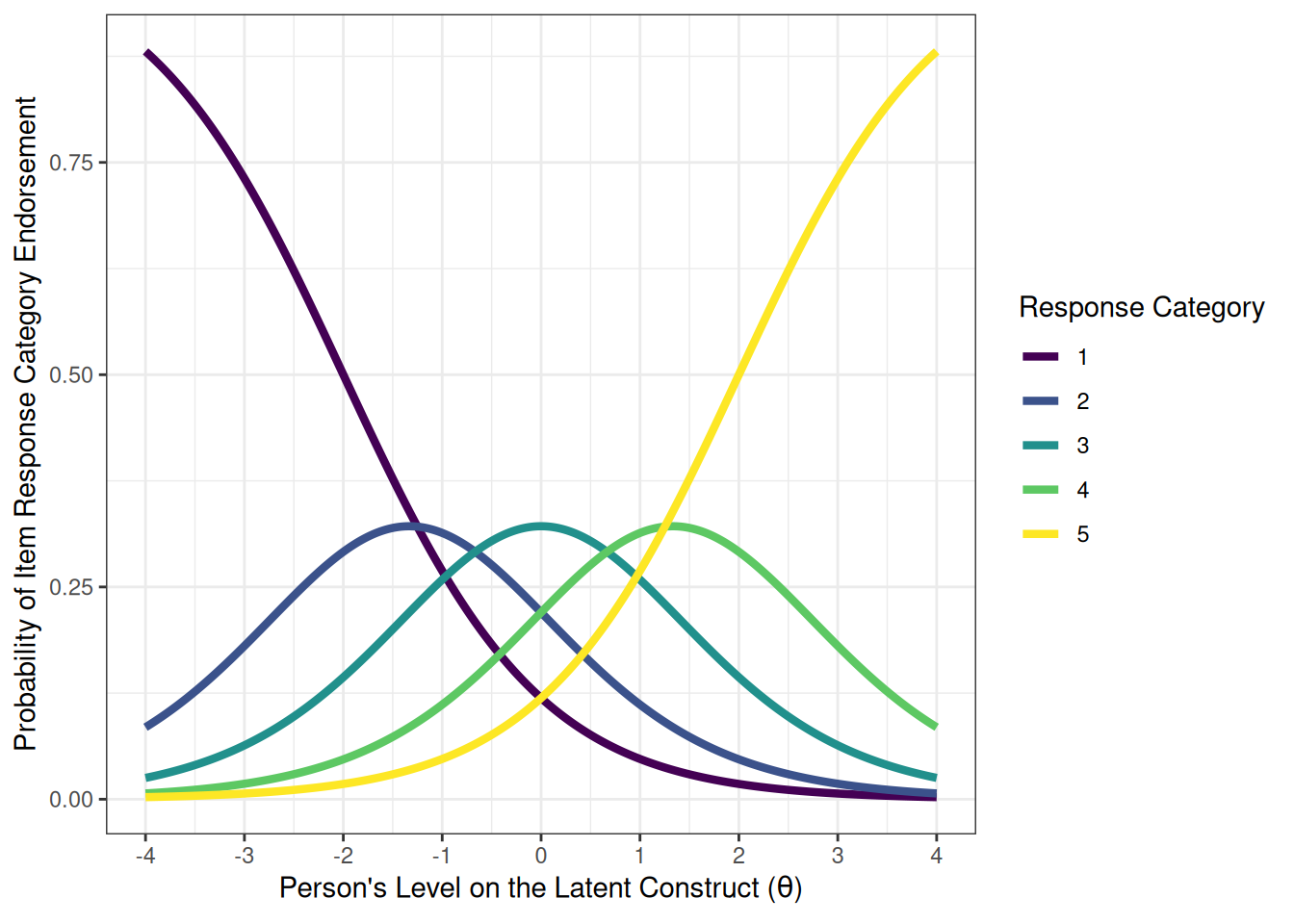
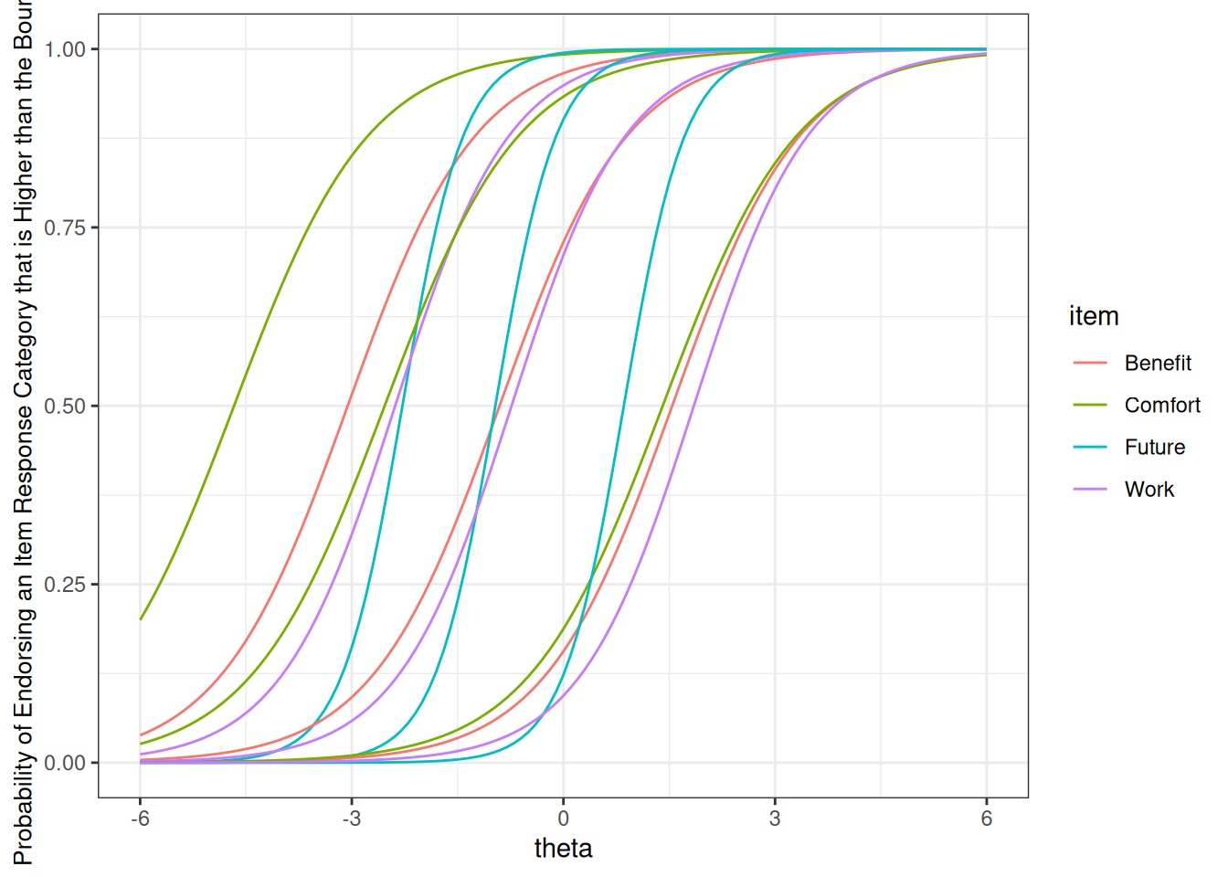
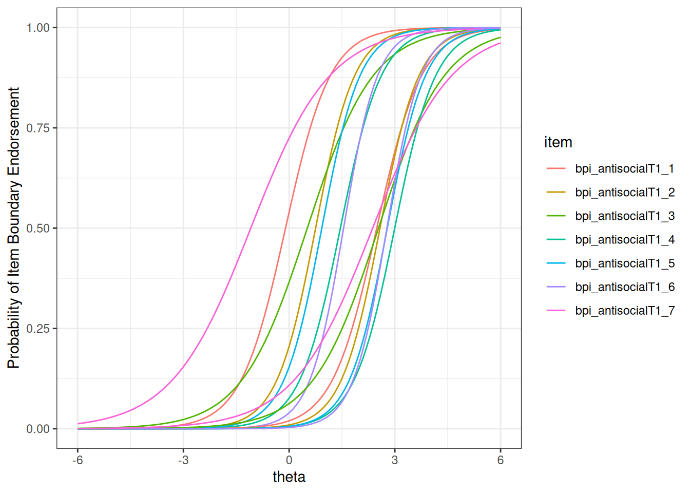
For example, see Figure 8.16 for an example of an item boundary characteristic curve for an item from a 5-level likert scale (based on a cumulative distribution). If an item has \(k\) response categories, it has \(k - 1\) thresholds. For example, an item with 5-level likert scale (1 = strongly disagree; 2 = disagree; 3 = neither agree nor disagree; 4 = agree; 5 = strongly agree) has 4 thresholds: one from 1–2, one from 2–3, one from 3–4, and one from 4–5. The item boundary characteristic curve is the probability that a person selects a response category higher than \(k\) of a polytomous item. As depicted, one likert scale item does equivalent work as 4 binary items. See Figure 8.17 for the same 5-level likert scale item plotted with an item response category characteristic curve (based on a static, non-cumulative distribution).
ggplot(polytomousItemBoundary_long, aes(theta, value, group =factor(boundary), color =factor(boundary))) +geom_line(linewidth =1.5) +labs(color ="Boundary") +scale_color_viridis_d() +scale_x_continuous(name =expression(paste("Person's Level on the Latent Construct (", theta, ")", sep ="")), breaks =-4:4) +scale_y_continuous(name ="Probability of Endorsing an Item Response Category that is Higher than the Boundary") +theme_bw() +theme(axis.title.y =element_text(size =9))
Figure 8.16: Item Boundary Characteristic Curves From Two-Parameter Graded Response Model in Item Response Theory.
Code
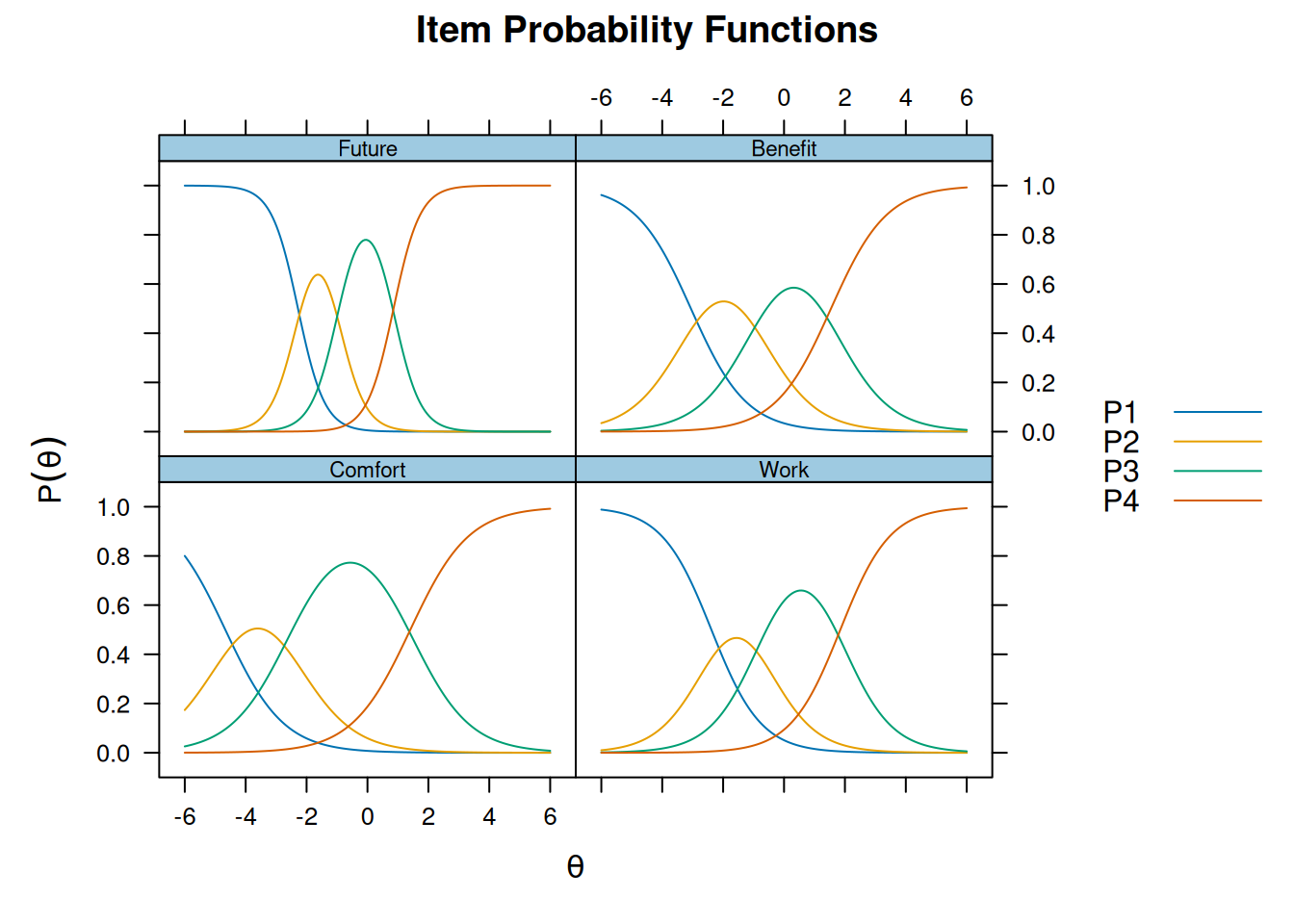
ggplot(polytomousItemResponseCategory_long, aes(theta, value, group =factor(responseCategory), color =factor(responseCategory))) +geom_line(linewidth =1.5) +labs(color ="Response Category") +scale_color_viridis_d() +scale_x_continuous(name =expression(paste("Person's Level on the Latent Construct (", theta, ")", sep ="")), breaks =-4:4) +scale_y_continuous(name ="Probability of Item Response Category Endorsement") +theme_bw()
Figure 8.17: Item Response Category Characteristic Curves From Two-Parameter Graded Response Model in Item Response Theory.
IRT does not handle continuous data well, with some exceptions (Chen et al., 2019) such as in a Bayesian framework (Bürkner, 2021). If you want to use continuous data, you might consider moving to a factor analysis framework.
8.1.5 Sample Size
Sample size requirements depend on the complexity of the model. A 1-parameter model often requires ~100 participants. A 2-parameter model often requires ~1,000 participants. A 3-parameter model often requires ~10,000 participants.
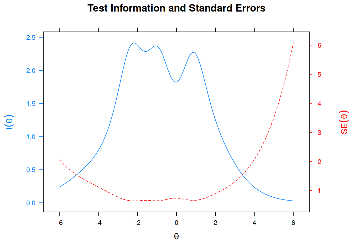
Based on an item’s difficulty and discrimination, we can calculate how much information each item provides. In IRT, information is how much measurement precision or consistency an item (or the measure) provides. In other words, information is the degree to which an item (or measure) reduces the standard error of measurement, that is, how much it reduces uncertainty of a person’s level on the construct. As a reminder (from Equation 4.11), the standard error of measurement is calculated as:
where \(\sigma_x = \text{standard deviation of observed scores on the item } x\), and \(r_{xx} = \text{reliability of the item } x\). The standard error of measurement is used to generate confidence intervals for people’s scores. In IRT, the standard error of measurement (at a given construct level) can be calculated as the inverse of the square root of the amount of test information at that construct level, as in Equation 8.8:
The petersenlab package (Petersen, 2025) contains the standardErrorIRT() function that estimates the standard error of measurement at a person’s level on the construct (theta) from the amount of information that the item (or test) provides.
The standard error of measurement tends to be higher (i.e., reliability/information tends to be lower) at the extreme levels of the construct where there are fewer items.
The formula for information for item \(i\) at construct level \(\theta\) in a Rasch model is in Equation 8.9:
where \(P_i(\theta)\) is the probability of getting a one instead of a zero on item \(i\) at a given level on the latent construct, and \(Q_i(\theta) = 1 - P_i(\theta)\).
The petersenlab package (Petersen, 2025) contains the itemInformation() function that estimates the amount of information an item provides as function of the item characteristics from the Rasch model and the person’s level on the construct (theta). To estimate the amount of information an item provides in a Rasch model, specify \(b\) and \(\theta\), while keeping the defaults for the other parameters.
Code
itemInformation <-function(a =1, b, c =0, d =1, theta){ P <-NULL information <-NULLfor(i in1:length(theta)){ P[i] <-fourPL(b = b, a = a, c = c, d = d, theta = theta[i]) information[i] <- ((a^2) * (P[i] - c)^2* (d - P[i])^2) / ((d - c)^2* P[i] * (1- P[i])) }return(information)}
Code
itemInformation(b, theta)
Code
itemInformation(b =1, theta =0)
[1] 0.1966119
The formula for information for item \(i\) at construct level \(\theta\) in a two-parameter logistic model is in Equation 8.10:
The petersenlab package (Petersen, 2025) contains the itemInformation() function that estimates the amount of information an item provides as function of the item characteristics from the two-parameter logistic model and the person’s level on the construct (theta). To estimate the amount of information an item provides in a two-parameter logistic model, specify \(a\), \(b\), and \(\theta\), while keeping the defaults for the other parameters.
Code
itemInformation(a, b, theta)
Code
itemInformation(a =0.6, b =0, theta =-1)
[1] 0.08236233
The formula for information for item \(i\) at construct level \(\theta\) in a three-parameter logistic model is in Equation 8.11:
The petersenlab package (Petersen, 2025) contains the itemInformation() function that estimates the amount of information an item provides as function of the item characteristics from the three-parameter logistic model and the person’s level on the construct (theta). To estimate the amount of information an item provides in a three-parameter logistic model, specify \(a\), \(b\), \(c\), and \(\theta\), while keeping the defaults for the other parameters.
Code
itemInformation(a, b, c, theta)
Code
itemInformation(a =0.8, b =-1, c = .25, theta =-1)
[1] 0.096
The formula for information for item \(i\) at construct level \(\theta\) in a four-parameter logistic model is in Equation 8.12:
The petersenlab package (Petersen, 2025) contains the itemInformation() function that estimates the amount of information an item provides as function of the item characteristics from the four-parameter logistic model and the person’s level on the construct (theta). To estimate the amount of information an item provides in a four-parameter logistic model, specify \(a\), \(b\), \(c\), \(d\), and \(\theta\).
Code
itemInformation(a, b, c, d, theta)
Code
itemInformation(a =1.5, b =1, c = .15, d =0.85, theta =3)
[1] 0.01503727
Reliability at a given level of the construct (\(\theta\)) can be estimated as in Equation 8.13:
where \(\sigma^2(\theta)\) is the variance of theta, which is fixed to one in most IRT models.
The petersenlab package (Petersen, 2025) contains the reliabilityIRT() function that estimates the amount of reliability an item or a measure provides as function of its information and the variance of people’s construct levels (\(\theta\)).
Code
reliabilityIRT <-function(information, varTheta =1){ information / (information + varTheta)}
Code
reliabilityIRT(information, varTheta =1)
Code
reliabilityIRT(10)
[1] 0.9090909
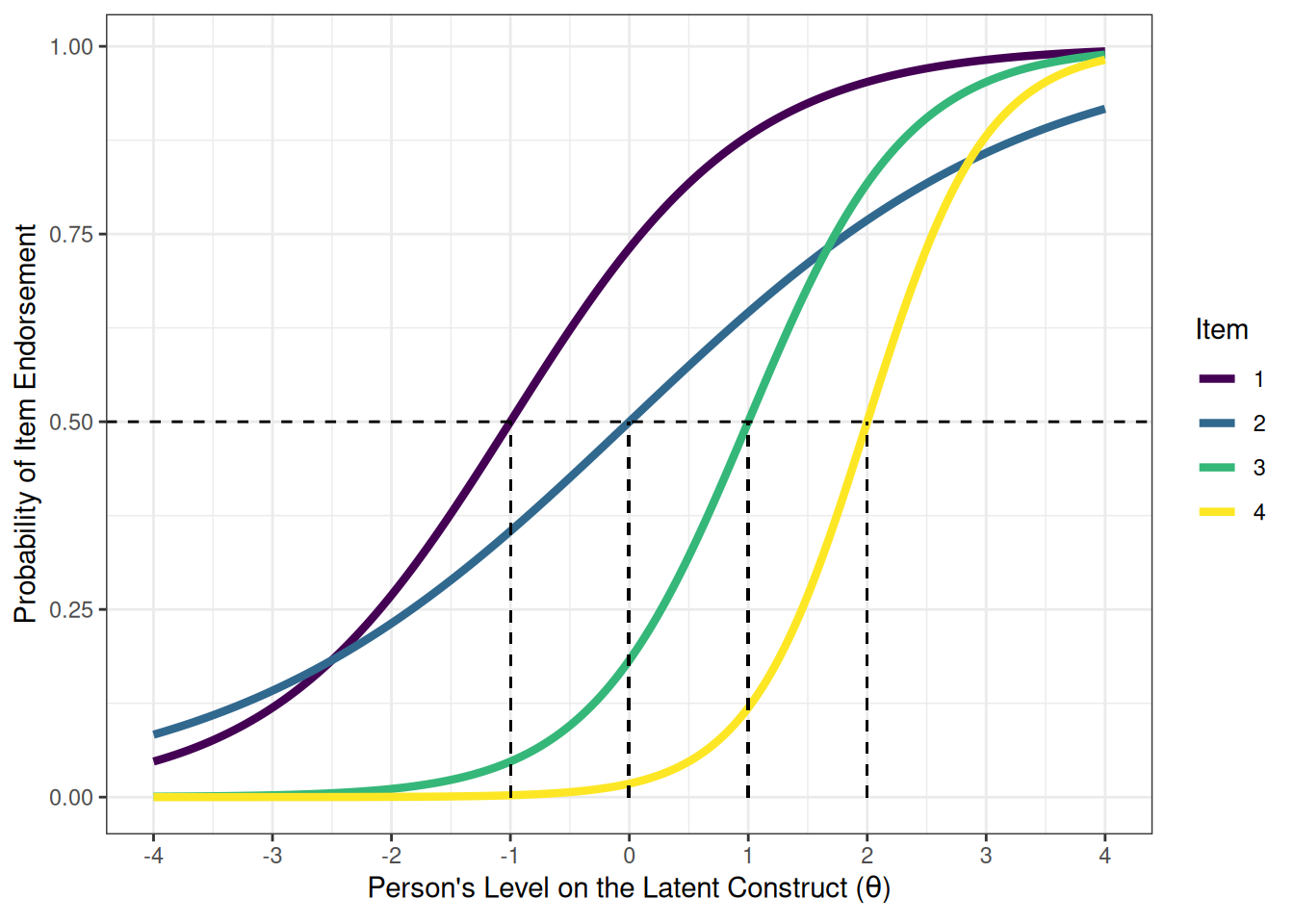
Consider some hypothetical items depicted with ICCs in Figure 8.18.
ggplot(irtReliability_long, aes(theta, value, group =factor(Item), color =factor(Item))) +geom_line(linewidth =1.5) +labs(color ="Item") +scale_color_viridis_d() +geom_hline(yintercept =0.5, linetype ="dashed") +geom_segment(aes(x = midpoint_item1, xend = midpoint_item1, y =0, yend =0.5), linewidth =0.5, col ="black", linetype ="dashed") +geom_segment(aes(x = midpoint_item2, xend = midpoint_item2, y =0, yend =0.5), linewidth =0.5, col ="black", linetype ="dashed") +geom_segment(aes(x = midpoint_item3, xend = midpoint_item3, y =0, yend =0.5), linewidth =0.5, col ="black", linetype ="dashed") +geom_segment(aes(x = midpoint_item4, xend = midpoint_item4, y =0, yend =0.5), linewidth =0.5, col ="black", linetype ="dashed") +scale_x_continuous(name =expression(paste("Person's Level on the Latent Construct (", theta, ")", sep ="")), breaks =-4:4) +scale_y_continuous(name ="Probability of Item Endorsement") +theme_bw()
Figure 8.18: Item Characteristic Curves From Two-Parameter Logistic Model in Item Response Theory. The dashed horizontal line indicates a probability of item endorsement of .50. The dashed vertical line is the item difficulty, i.e., the person’s level on the construct (the location on the x-axis) at the inflection point of the item characteristic curve. In a two-parameter logistic model, the inflection point corresponds to the probability of item endorsement is 50%. Thus, in a two-parameter logistic model, the difficulty of an item is the person’s level on the construct where the probability of endorsing the item is 50%.
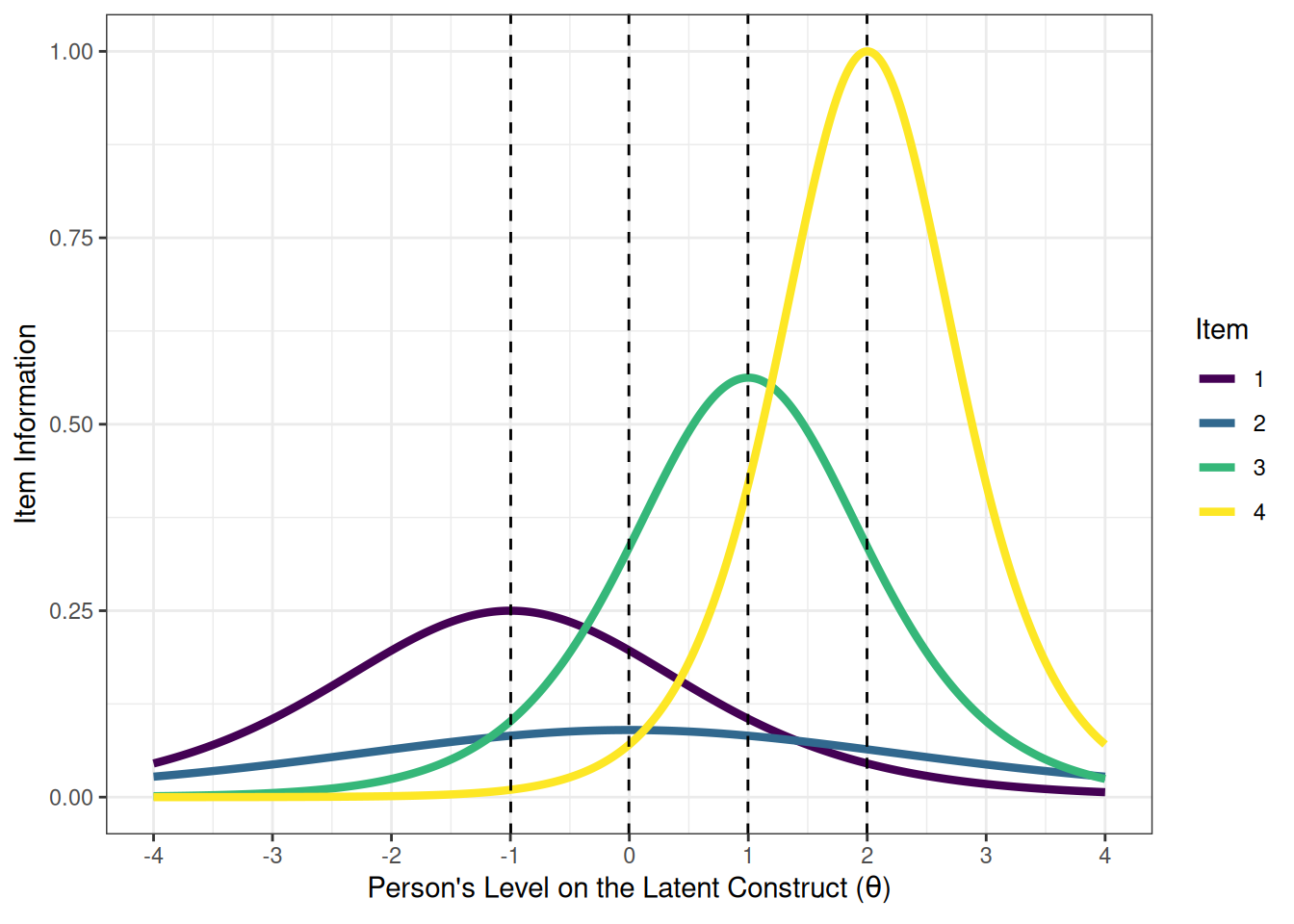
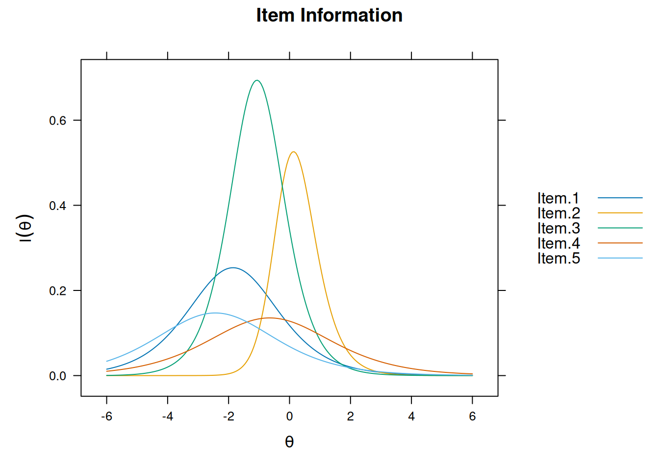
We can present the ICC in terms of an item information curve (see Figure 8.19). On the x-axis, the information peak is located at the difficulty/severity of the item. The higher the discrimination, the higher the information peak on the y-axis.
Figure 8.19: Item Information From Two-Parameter Logistic Model in Item Response Theory. The dashed vertical line is the item difficulty, which is located at the peak of the item information curve.
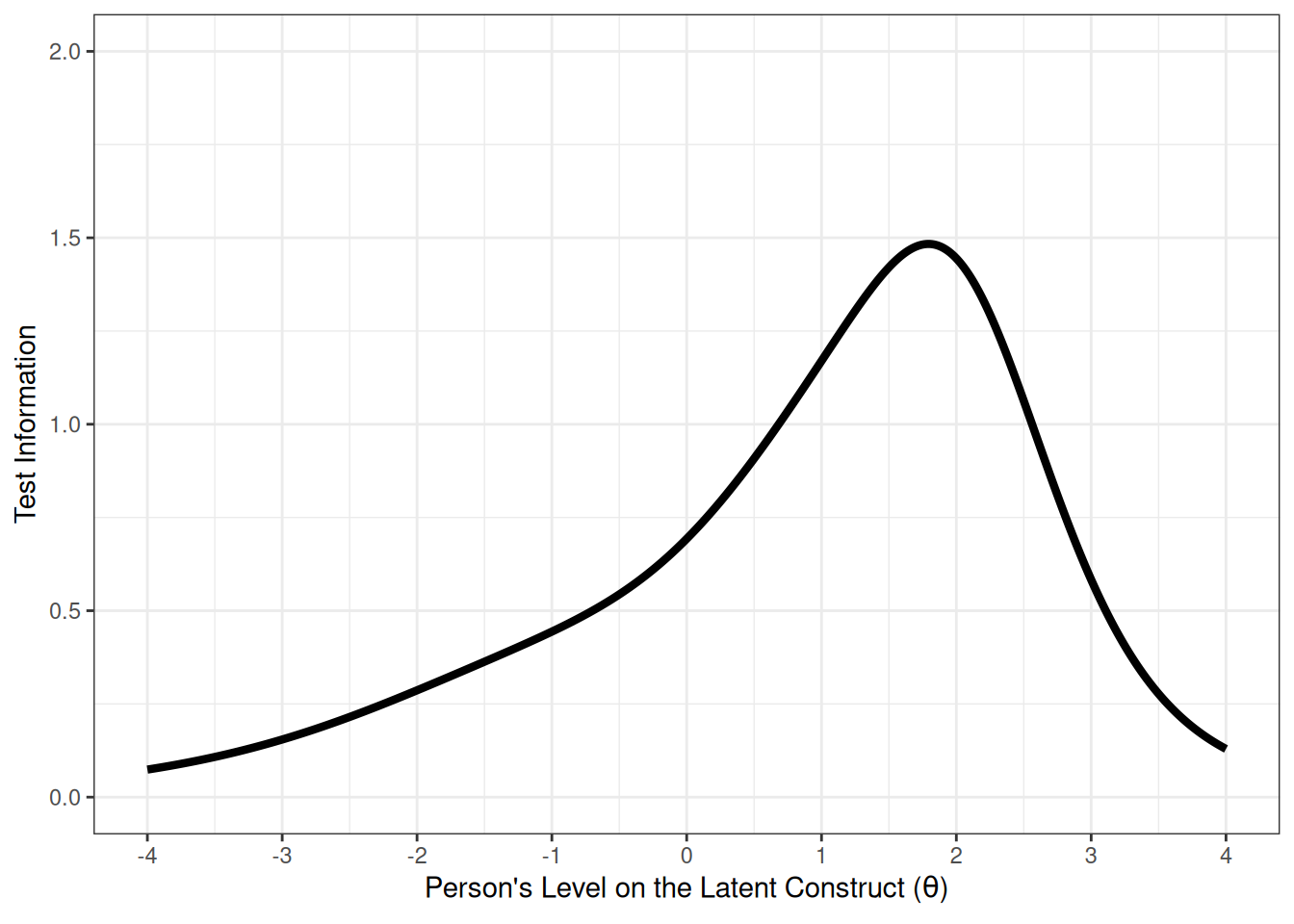
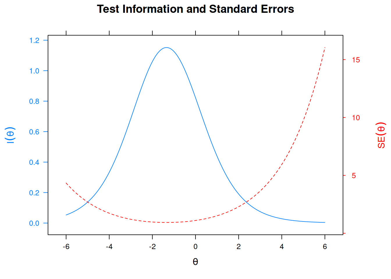
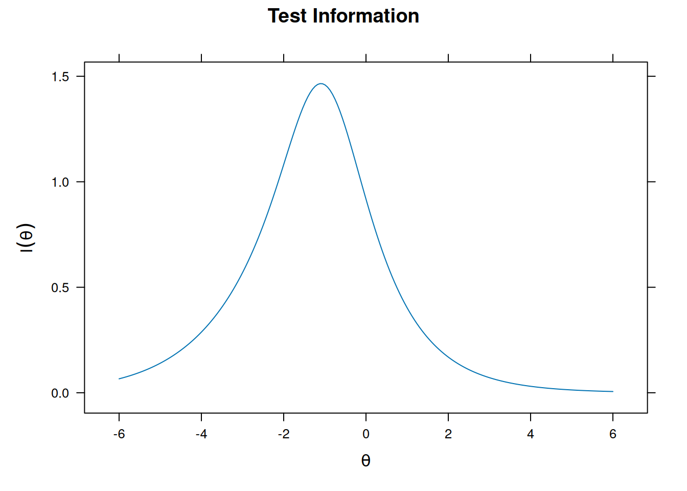
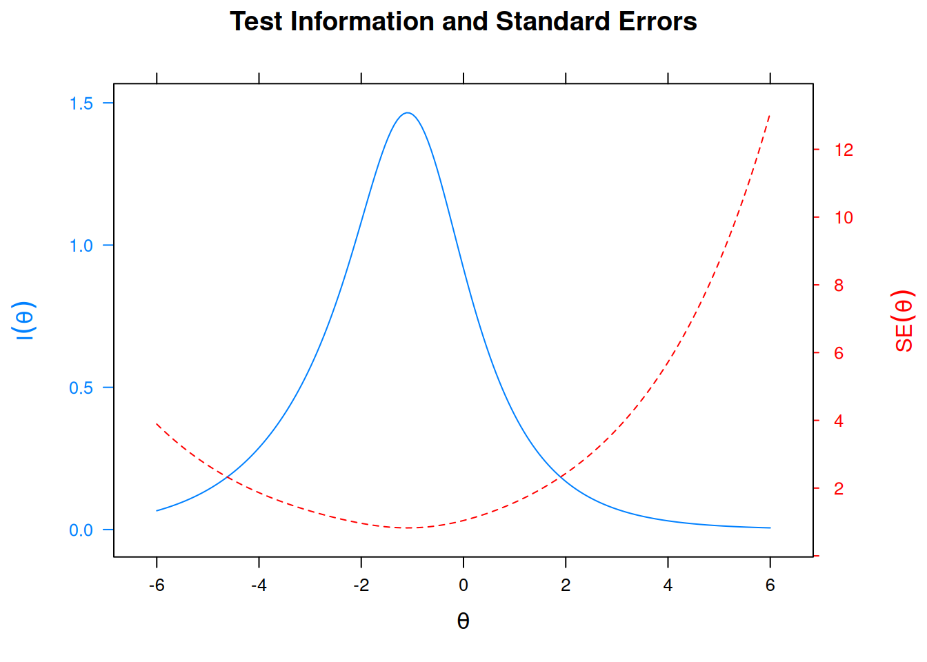
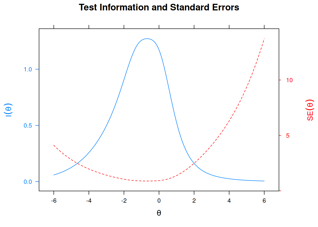
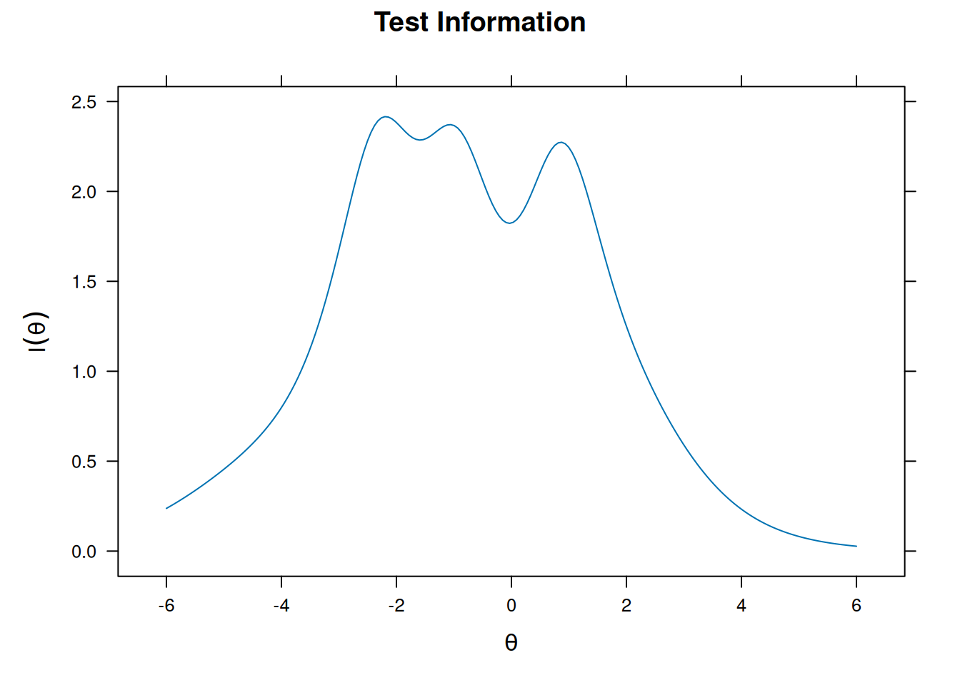
We can aggregate (sum) information across items to determine how much information the measure as a whole provides. This is called the test information curve (see Figure 8.20). Note that we get more information from likert/multiple response items compared to binary/dichotomous items. Having 10 items with a 5-level response scale yields as much information as 40 dichotomous items.
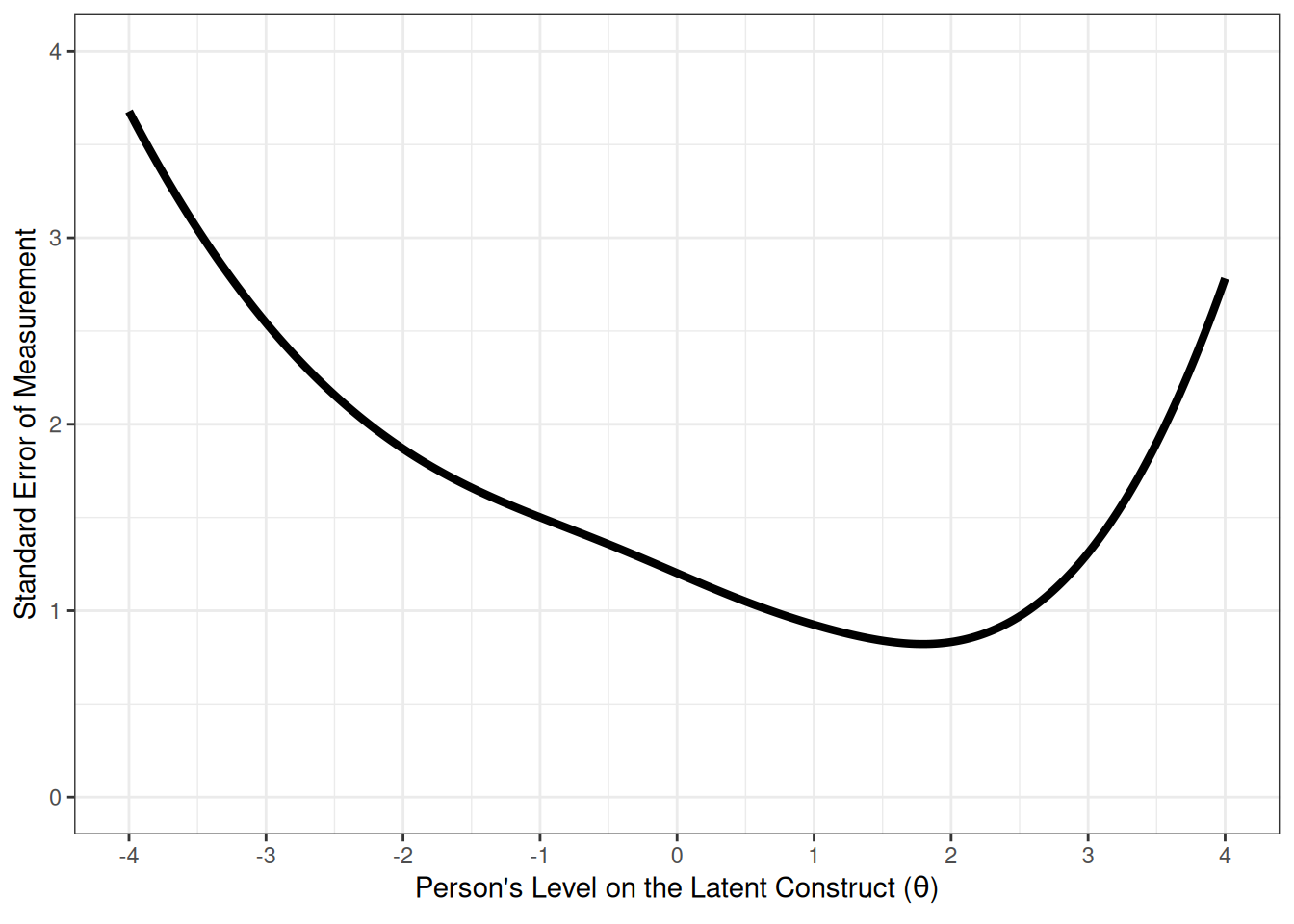
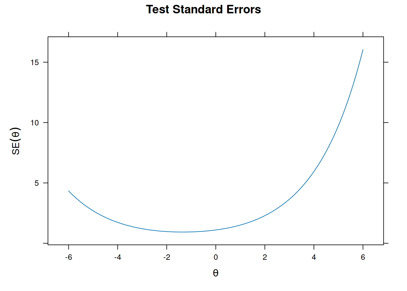
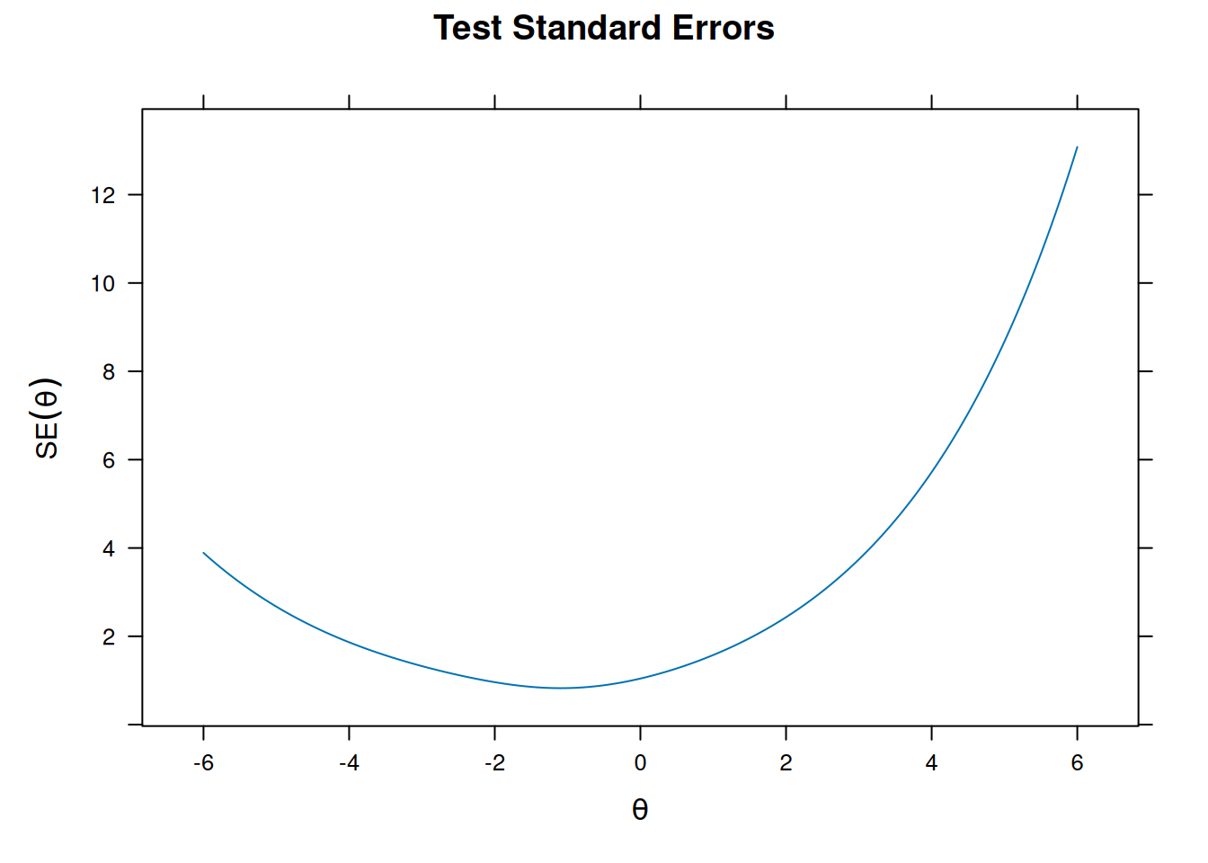
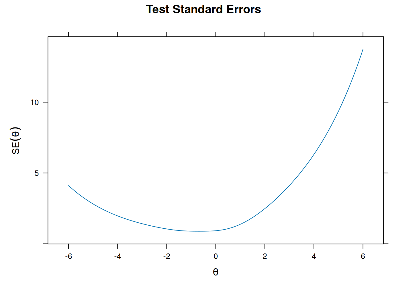
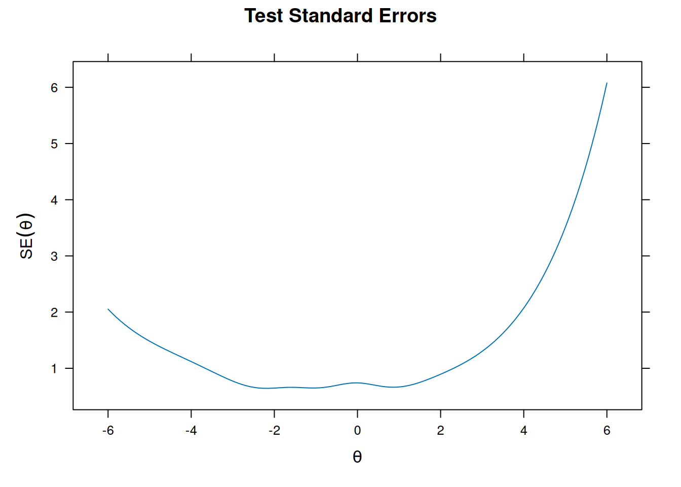
ggplot(irtInformation, aes(theta, standardError)) +geom_line(linewidth =1.5) +scale_color_viridis_d() +scale_x_continuous(name =expression(paste("Person's Level on the Latent Construct (", theta, ")", sep ="")), breaks =-4:4) +scale_y_continuous(name ="Standard Error of Measurement", limits =c(0,4)) +theme_bw()
Figure 8.21: Test Standard Error of Measurement From Two-Parameter Logistic Model in Item Response Theory.
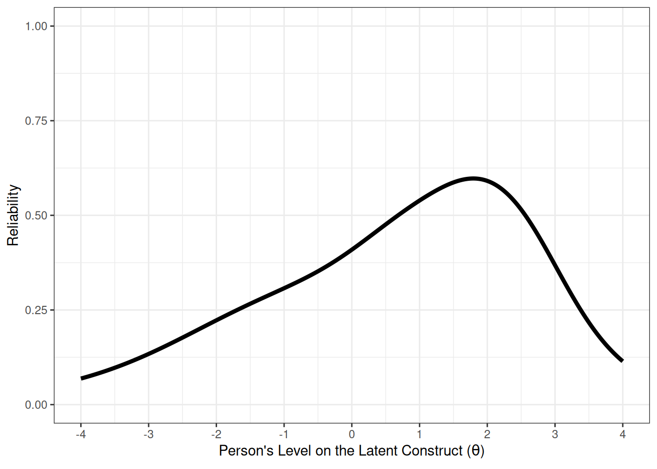
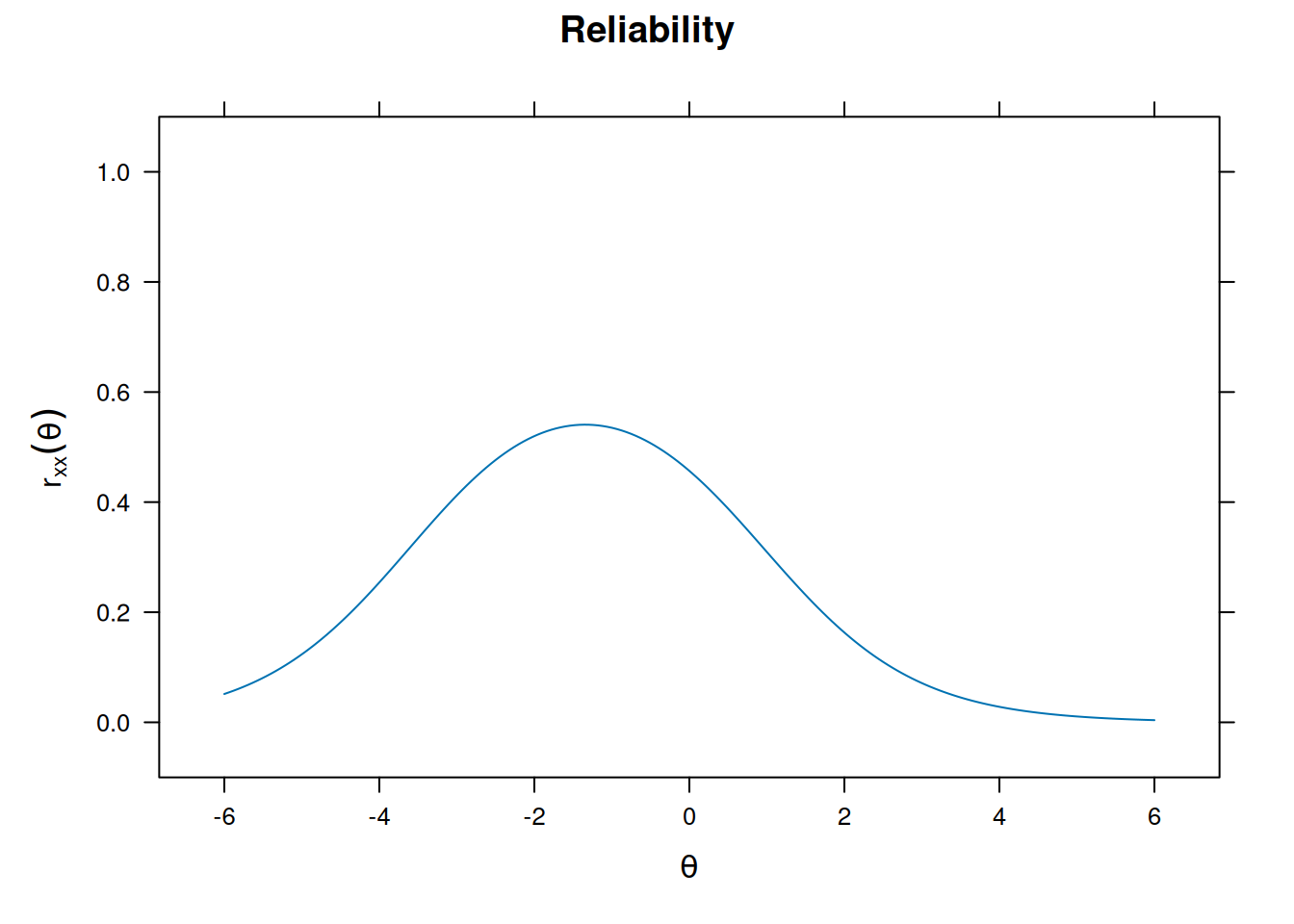
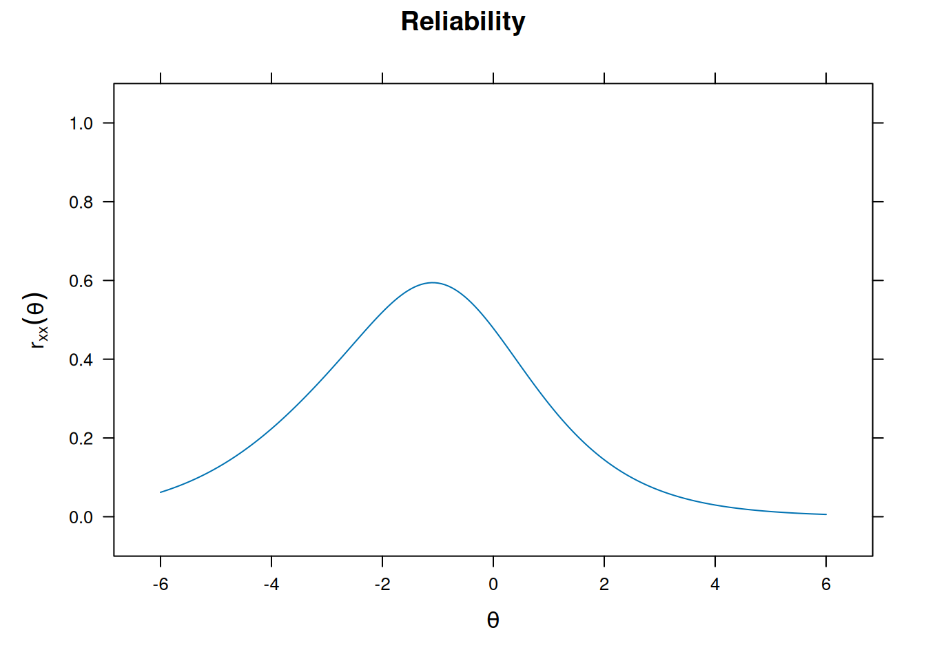
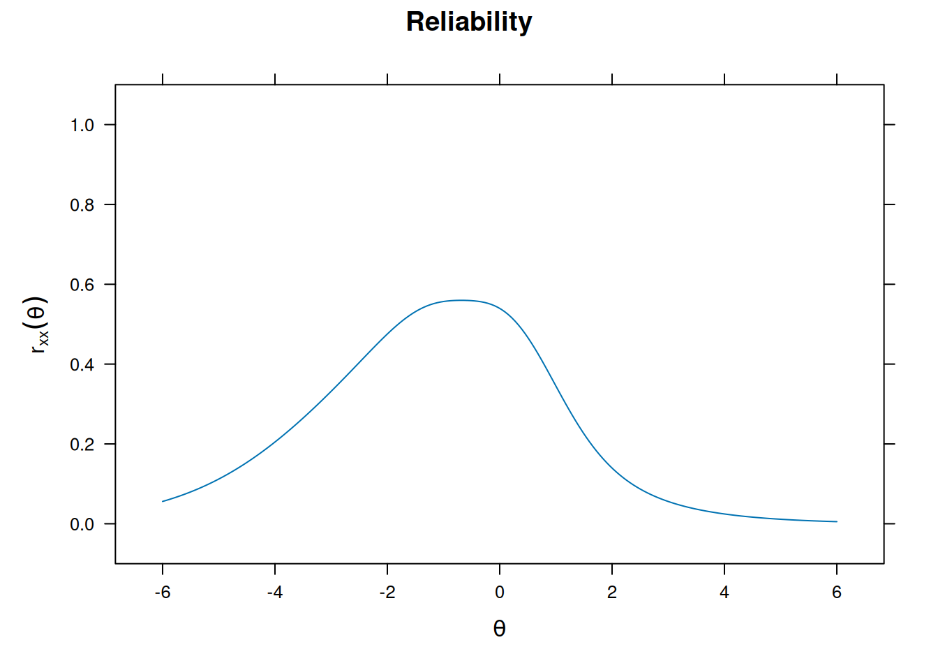
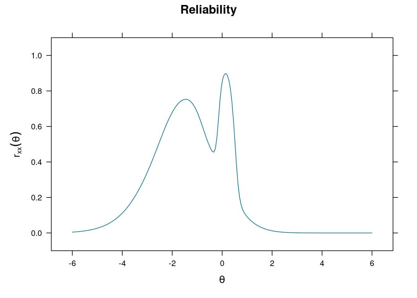
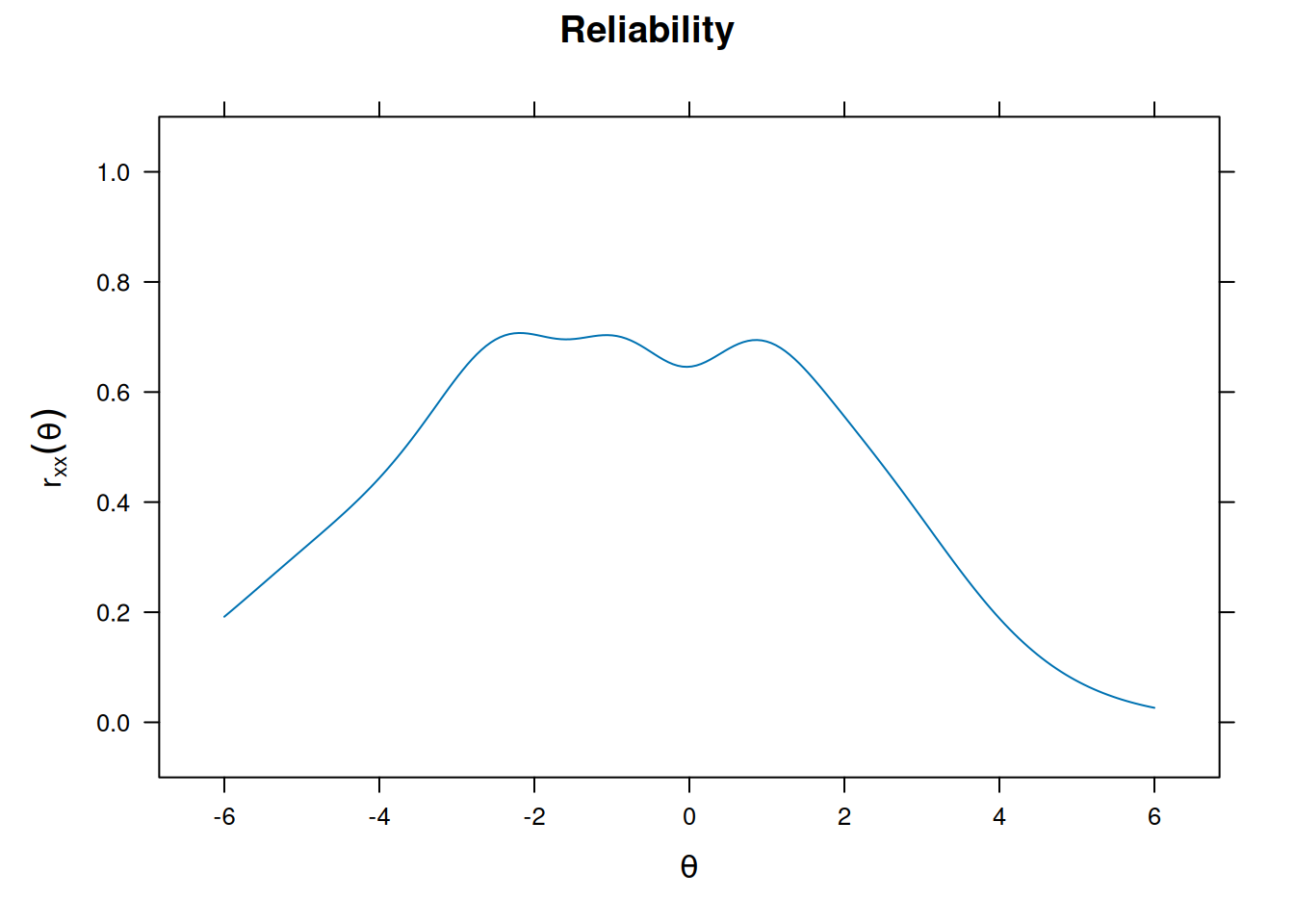
Based on test information, we can estimate the reliability (see Figure 8.22). Notice how the degree of (un)reliability differs at different construct levels.
Figure 8.22: Test Reliability From Two-Parameter Logistic Model in Item Response Theory.
8.1.7 Efficient Assessment
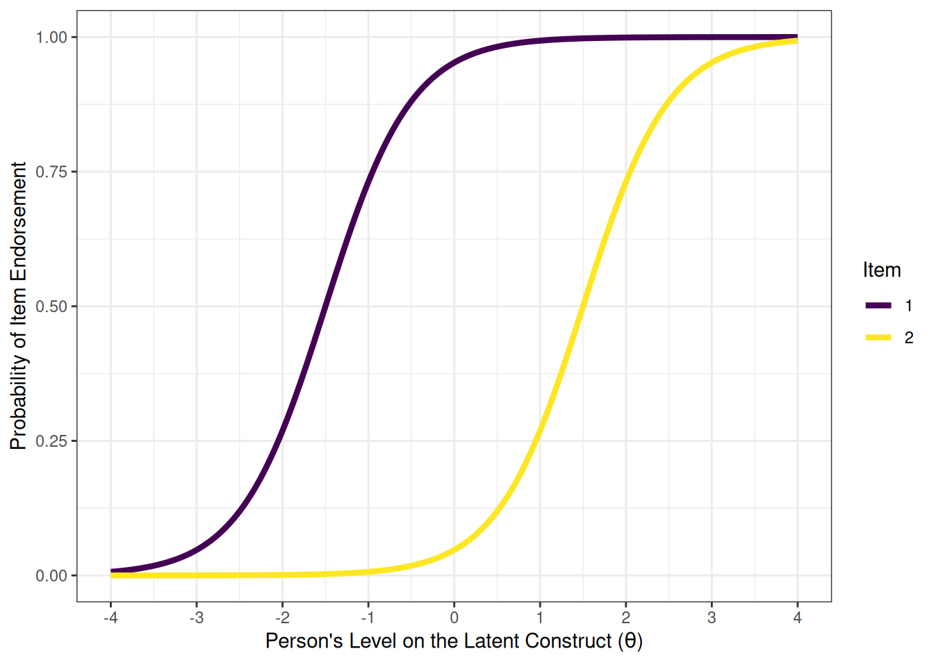
One of the benefits of IRT is for item selection to develop brief assessments. For instance, you could use two items to estimate where the person is on the construct: low, middle, or high (see Figure 8.23). If the responses to the two items do not meet expectations, for instance, the person passes the difficult item but fails the easy item, we would keep assessing additional items to determine their level on the construct. If two items perform similarly, that is, they have the same difficulty and discrimination, they are redundant, and we can sacrifice one of them. This leads to greater efficiency and better measurement in terms of reliability and validity. For more information on designing and evaluating short forms compared to their full-scale counterparts, see Smith et al. (2000).
ggplot(efficientAssessment_long, aes(theta, value, group =factor(Item), color =factor(Item))) +geom_line(linewidth =1.5) +labs(color ="Item") +scale_color_viridis_d() +scale_x_continuous(name =expression(paste("Person's Level on the Latent Construct (", theta, ")", sep ="")), breaks =-4:4) +scale_y_continuous(name ="Probability of Item Endorsement") +theme_bw()
Figure 8.23: Visual Representation of an Efficient Assessment Based on Item Characteristic Curves from Two-Parameter Logistic Model in Item Response Theory.
IRT forms the basis of computerized adaptive testing, which is discussed in Chapter 21. As discussed earlier, briefer measures can increase reliability and validity of measurement if the items are tailored to the ability level of the participant. The idea of adaptive testing is that, instead of having a standard scale for all participants, the items adapt to each person. An example of a measure that has used computerized adaptive testing is the Graduate Record Examination (GRE).
With adaptive testing, it is important to develop a comprehensive item bank that spans the difficulty range of interest. The starting construct level is the 50th percentile. If the respondent gets the first item correct, it moves to the next item that would provide the most information for the person, based on a split of the remaining sample (e.g., 75th percentile). And so on… The goal of adaptive testing is to find the construct level where the respondent keeps getting items right and wrong 50% of the time. Adaptive testing is a promising approach that saves time because it tailors which items are administered to which person (based on their construct level) to get the most reliable estimate in the shortest time possible. However, it assumes that if you get a more difficult item correct, that you would have gotten easier items correct, which might not be true in all contexts (especially for constructs that are not unidimensional).
Although most uses of IRT have been in cognitive and educational testing, IRT may also benefit other domains of assessment including clinical assessment (Gibbons et al., 2016; Reise & Waller, 2009; Thomas, 2019).
8.1.7.1 A Good Measure
According to IRT a good measure should:
fit your goals of the assessment, in terms of the range of interest regarding levels on the construct,
have good items that yield lots of information, and
have a good set of items that densely cover the construct within the range of interest, without redundancy.
First, a good measure should fit your goals of the assessment, in terms of the “range of interest” or the “target range” of levels on the construct. For instance, if your goal is to perform diagnosis, you would only care about the high end of the construct (e.g., 1–3 standard deviations above the mean)—there is no use discriminating between “nothing”, “almost nothing”, and “a little bit.” For secondary prevention, i.e., early identification of risk to prevent something from getting worse, you would be interested in finding people with elevated risk—e.g., you would need to know who is 1 or more standard deviations above the mean, but you would not need to discriminate beyond that. For assessing individual differences, you would want items that discriminate across the full range, including at the lower end. The items’ difficulty should span the range of interest.
Second, a good measure should have good items that yield lots of information. For example, the items should have strong discrimination, that is, the items are strongly related to the construct. The items should have sufficient variability in responses. This can be achieved by having items with more response options (e.g., likert/multiple choice items, as opposed to binary items), items that differ in difficulty, and (at least some) items that are not too difficult or too easy (to avoid ceiling/floor effects).
Third, a good measure should have a good set of items that densely cover the construct within the range of interest, without redundancy. The items should not have the same difficulty or they would be considered redundant, and one of the redundant items could be dropped. The items’ difficulty should densely cover the construct within the range of interest. For instance, if the construct range of interest is 1–2 standard deviations above the mean, the items should have difficulty that densely cover this range (e.g., 1.0, 1.05, 1.10, 1.15, 1.20, 1.25, 1.30, …, 2.0).
With items that (1) span the range of interest, (2) have high discrimination and information, and (3) densely cover the range of interest without redundancy, the measure should have a high information in the range of interest. This would allow it to efficiently and accurately assess the construct for the intended purpose.
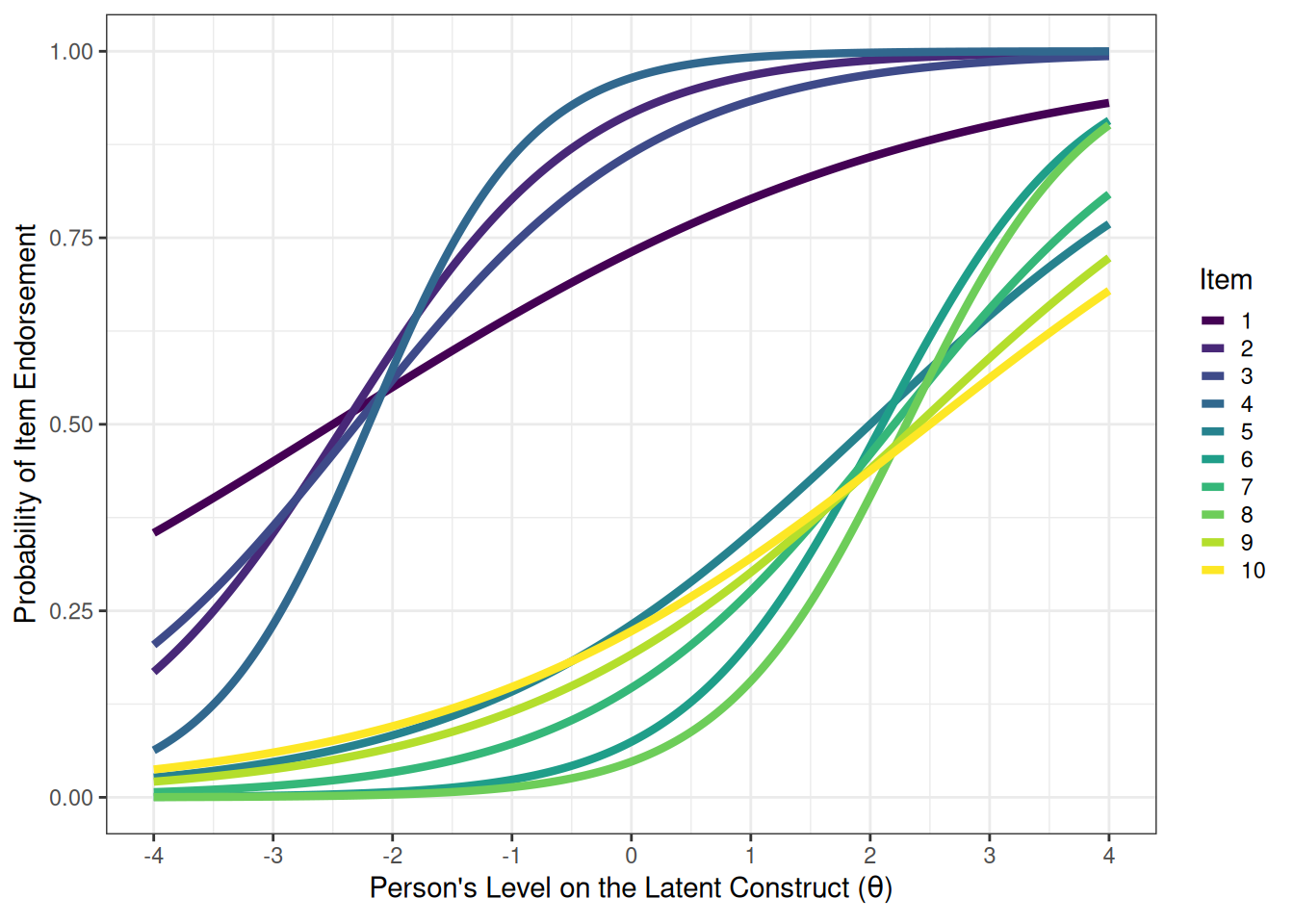
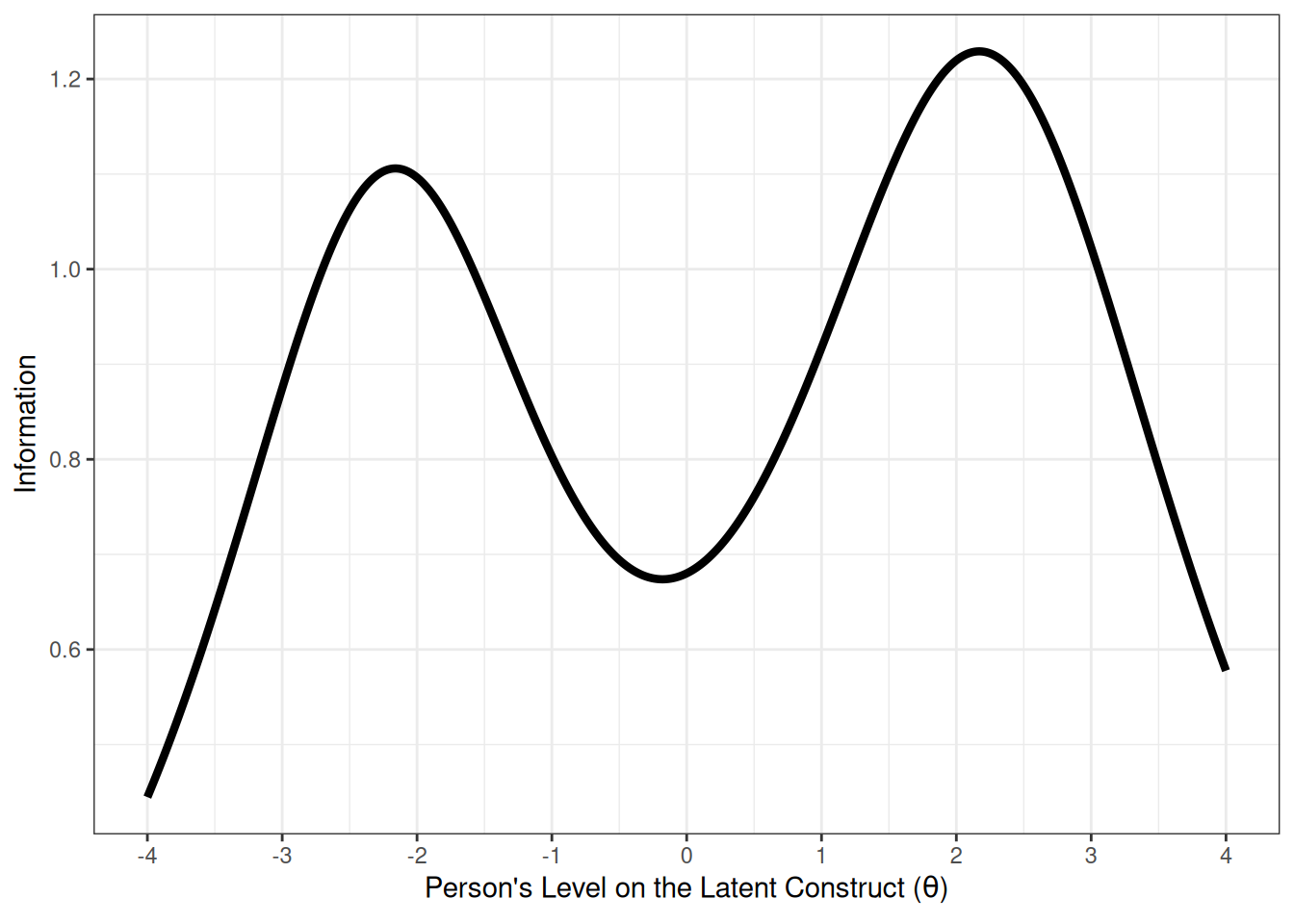
An example of a bad measure for assessing the full range of individual differences is depicted in terms of ICCs in Figure 8.24 and in terms of test information in Figure 8.25. The measure performs poorly for the intended purpose, because its items do not (a) span the range of interest (−3 to 3 standard deviations from the mean of the latent construct), (b) have high discrimination and information, and (c) densely cover the range of interest without redundancy.
Code
badMeasure <- badMeasureInfo <-data.frame(theta =seq(from =-4, to =4, length.out =1000))badMeasure$item1 <-fourPL(b =-2.5, a =0.4, theta = badMeasure$theta)badMeasure$item2 <-fourPL(b =-2.4, a =1, theta = badMeasure$theta)badMeasure$item3 <-fourPL(b =-2.3, a =0.8, theta = badMeasure$theta)badMeasure$item4 <-fourPL(b =-2.2, a =1.5, theta = badMeasure$theta)badMeasure$item5 <-fourPL(b =2.0, a =0.6, theta = badMeasure$theta)badMeasure$item6 <-fourPL(b =2.1, a =1.2, theta = badMeasure$theta)badMeasure$item7 <-fourPL(b =2.2, a =0.8, theta = badMeasure$theta)badMeasure$item8 <-fourPL(b =2.3, a =1.3, theta = badMeasure$theta)badMeasure$item9 <-fourPL(b =2.4, a =0.6, theta = badMeasure$theta)badMeasure$item10 <-fourPL(b =2.5, a =0.5, theta = badMeasure$theta)badMeasureInfo$info1 <-itemInformation(b =-2.5, a =0.4, theta = badMeasureInfo$theta)badMeasureInfo$info2 <-itemInformation(b =-2.4, a =1, theta = badMeasureInfo$theta)badMeasureInfo$info3 <-itemInformation(b =-2.3, a =0.8, theta = badMeasureInfo$theta)badMeasureInfo$info4 <-itemInformation(b =-2.2, a =1.5, theta = badMeasureInfo$theta)badMeasureInfo$info5 <-itemInformation(b =2.0, a =0.6, theta = badMeasureInfo$theta)badMeasureInfo$info6 <-itemInformation(b =2.1, a =1.2, theta = badMeasureInfo$theta)badMeasureInfo$info7 <-itemInformation(b =2.2, a =0.8, theta = badMeasureInfo$theta)badMeasureInfo$info8 <-itemInformation(b =2.3, a =1.3, theta = badMeasureInfo$theta)badMeasureInfo$info9 <-itemInformation(b =2.4, a =0.6, theta = badMeasureInfo$theta)badMeasureInfo$info10 <-itemInformation(b =2.5, a =0.5, theta = badMeasureInfo$theta)badMeasureInfo$information <-rowSums(badMeasureInfo[,paste("info", 1:10, sep ="")])badMeasure_long <-pivot_longer(badMeasure, cols = item1:item10) %>%rename(item = name)badMeasure_long$Item <-NAbadMeasure_long$Item[which(badMeasure_long$item =="item1")] <-1badMeasure_long$Item[which(badMeasure_long$item =="item2")] <-2badMeasure_long$Item[which(badMeasure_long$item =="item3")] <-3badMeasure_long$Item[which(badMeasure_long$item =="item4")] <-4badMeasure_long$Item[which(badMeasure_long$item =="item5")] <-5badMeasure_long$Item[which(badMeasure_long$item =="item6")] <-6badMeasure_long$Item[which(badMeasure_long$item =="item7")] <-7badMeasure_long$Item[which(badMeasure_long$item =="item8")] <-8badMeasure_long$Item[which(badMeasure_long$item =="item9")] <-9badMeasure_long$Item[which(badMeasure_long$item =="item10")] <-10
Code
ggplot(badMeasure_long, aes(theta, value, group =factor(Item), color =factor(Item))) +geom_line(linewidth =1.5) +labs(color ="Item") +scale_color_viridis_d() +scale_x_continuous(name =expression(paste("Person's Level on the Latent Construct (", theta, ")", sep ="")), breaks =-4:4) +scale_y_continuous(name ="Probability of Item Endorsement") +theme_bw() +theme(legend.key.size =unit(0.15, "in"))
Figure 8.24: Visual Representation of a Bad Measure Based on Item Characteristic Curves of Items From a Bad Measure Estimated from Two-Parameter Logistic Model in Item Response Theory.
Figure 8.25: Visual Representation of a Bad Measure Based on the Test Information Curve.
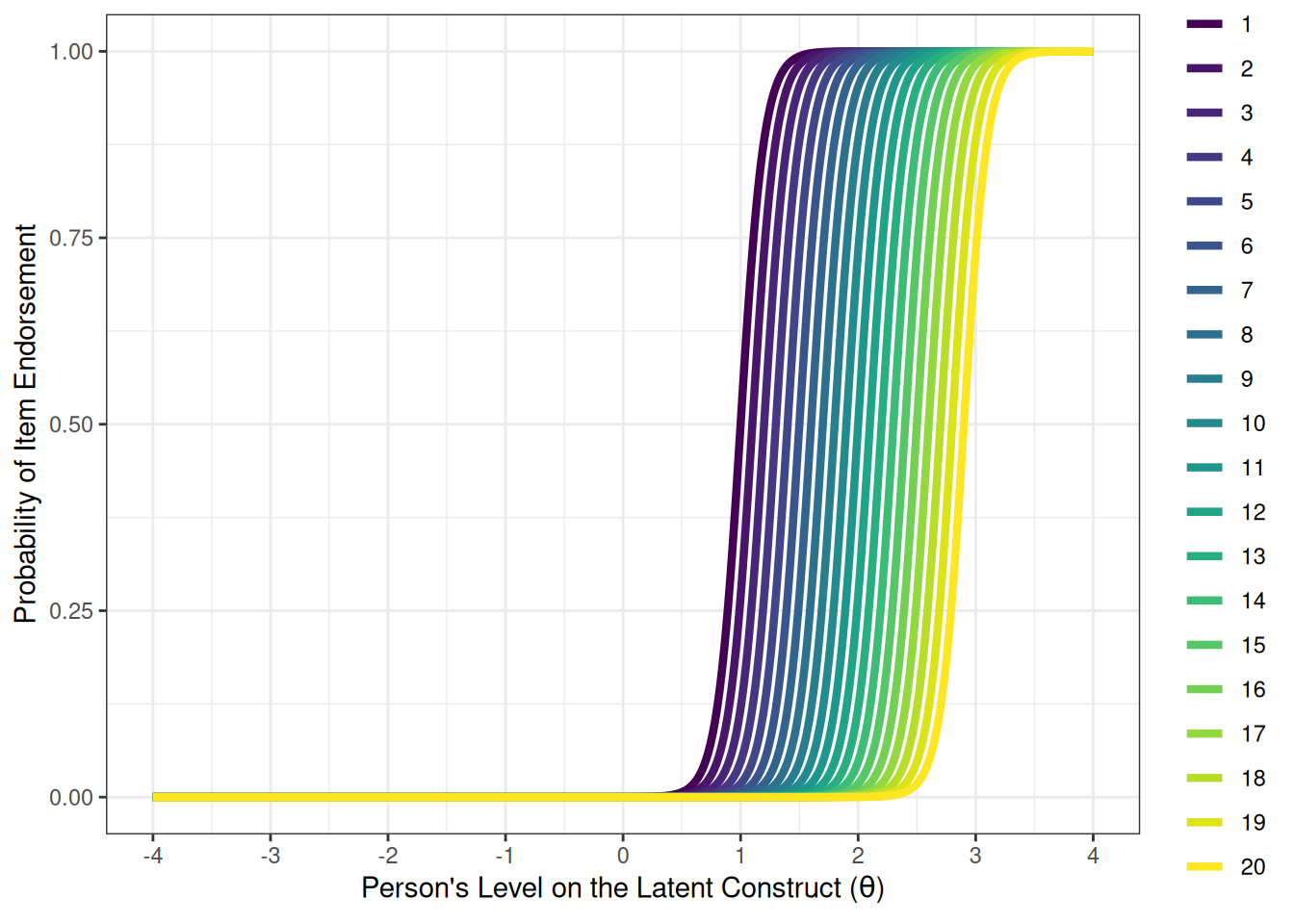
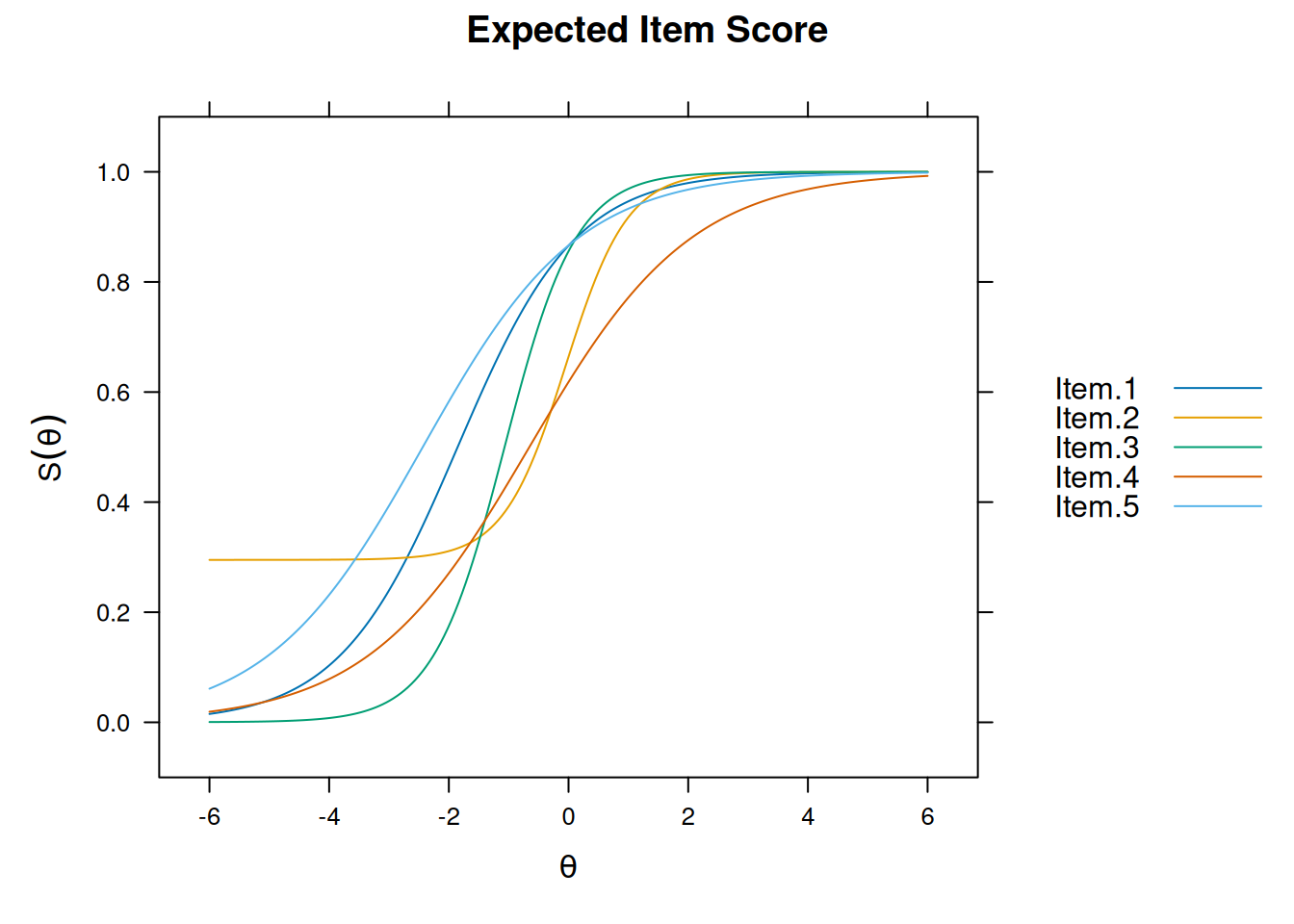
An example of a good measure for distinguishing clinical-range versus sub-clinical range is depicted in terms of ICCs in Figure 8.26 and in terms of test information in Figure 8.27. The measure is good for the intended purpose, in terms of having items that (a) span the range of interest (1–3 standard deviations above the mean of the latent construct), (b) have high discrimination and information, and (c) densely cover the range of interest without redundancy.
Code
goodMeasure <- goodMeasureInfo <-data.frame(theta =seq(from =-4, to =4, length.out =1000))goodMeasure$item1 <-fourPL(b =1.0, a =10, theta = goodMeasure$theta)goodMeasure$item2 <-fourPL(b =1.1, a =10, theta = goodMeasure$theta)goodMeasure$item3 <-fourPL(b =1.2, a =10, theta = goodMeasure$theta)goodMeasure$item4 <-fourPL(b =1.3, a =10, theta = goodMeasure$theta)goodMeasure$item5 <-fourPL(b =1.4, a =10, theta = goodMeasure$theta)goodMeasure$item6 <-fourPL(b =1.5, a =10, theta = goodMeasure$theta)goodMeasure$item7 <-fourPL(b =1.6, a =10, theta = goodMeasure$theta)goodMeasure$item8 <-fourPL(b =1.7, a =10, theta = goodMeasure$theta)goodMeasure$item9 <-fourPL(b =1.8, a =10, theta = goodMeasure$theta)goodMeasure$item10 <-fourPL(b =1.9, a =10, theta = goodMeasure$theta)goodMeasure$item11 <-fourPL(b =2.0, a =10, theta = goodMeasure$theta)goodMeasure$item12 <-fourPL(b =2.1, a =10, theta = goodMeasure$theta)goodMeasure$item13 <-fourPL(b =2.2, a =10, theta = goodMeasure$theta)goodMeasure$item14 <-fourPL(b =2.3, a =10, theta = goodMeasure$theta)goodMeasure$item15 <-fourPL(b =2.4, a =10, theta = goodMeasure$theta)goodMeasure$item16 <-fourPL(b =2.5, a =10, theta = goodMeasure$theta)goodMeasure$item17 <-fourPL(b =2.6, a =10, theta = goodMeasure$theta)goodMeasure$item18 <-fourPL(b =2.7, a =10, theta = goodMeasure$theta)goodMeasure$item19 <-fourPL(b =2.8, a =10, theta = goodMeasure$theta)goodMeasure$item20 <-fourPL(b =2.9, a =10, theta = goodMeasure$theta)goodMeasureInfo$info1 <-itemInformation(b =1.0, a =10, theta = goodMeasureInfo$theta)goodMeasureInfo$info2 <-itemInformation(b =1.1, a =10, theta = goodMeasureInfo$theta)goodMeasureInfo$info3 <-itemInformation(b =1.2, a =10, theta = goodMeasureInfo$theta)goodMeasureInfo$info4 <-itemInformation(b =1.3, a =10, theta = goodMeasureInfo$theta)goodMeasureInfo$info5 <-itemInformation(b =1.4, a =10, theta = goodMeasureInfo$theta)goodMeasureInfo$info6 <-itemInformation(b =1.5, a =10, theta = goodMeasureInfo$theta)goodMeasureInfo$info7 <-itemInformation(b =1.6, a =10, theta = goodMeasureInfo$theta)goodMeasureInfo$info8 <-itemInformation(b =1.7, a =10, theta = goodMeasureInfo$theta)goodMeasureInfo$info9 <-itemInformation(b =1.8, a =10, theta = goodMeasureInfo$theta)goodMeasureInfo$info10 <-itemInformation(b =1.9, a =10, theta = goodMeasureInfo$theta)goodMeasureInfo$info11 <-itemInformation(b =2.0, a =10, theta = goodMeasureInfo$theta)goodMeasureInfo$info12 <-itemInformation(b =2.1, a =10, theta = goodMeasureInfo$theta)goodMeasureInfo$info13 <-itemInformation(b =2.2, a =10, theta = goodMeasureInfo$theta)goodMeasureInfo$info14 <-itemInformation(b =2.3, a =10, theta = goodMeasureInfo$theta)goodMeasureInfo$info15 <-itemInformation(b =2.4, a =10, theta = goodMeasureInfo$theta)goodMeasureInfo$info16 <-itemInformation(b =2.5, a =10, theta = goodMeasureInfo$theta)goodMeasureInfo$info17 <-itemInformation(b =2.6, a =10, theta = goodMeasureInfo$theta)goodMeasureInfo$info18 <-itemInformation(b =2.7, a =10, theta = goodMeasureInfo$theta)goodMeasureInfo$info19 <-itemInformation(b =2.8, a =10, theta = goodMeasureInfo$theta)goodMeasureInfo$info20 <-itemInformation(b =2.9, a =10, theta = goodMeasureInfo$theta)goodMeasureInfo$information <-rowSums(goodMeasureInfo[,paste("info", 1:20, sep ="")])goodMeasure_long <-pivot_longer(goodMeasure, cols = item1:item20) %>%rename(item = name)goodMeasure_long$Item <-NAgoodMeasure_long$Item[which(goodMeasure_long$item =="item1")] <-1goodMeasure_long$Item[which(goodMeasure_long$item =="item2")] <-2goodMeasure_long$Item[which(goodMeasure_long$item =="item3")] <-3goodMeasure_long$Item[which(goodMeasure_long$item =="item4")] <-4goodMeasure_long$Item[which(goodMeasure_long$item =="item5")] <-5goodMeasure_long$Item[which(goodMeasure_long$item =="item6")] <-6goodMeasure_long$Item[which(goodMeasure_long$item =="item7")] <-7goodMeasure_long$Item[which(goodMeasure_long$item =="item8")] <-8goodMeasure_long$Item[which(goodMeasure_long$item =="item9")] <-9goodMeasure_long$Item[which(goodMeasure_long$item =="item10")] <-10goodMeasure_long$Item[which(goodMeasure_long$item =="item11")] <-11goodMeasure_long$Item[which(goodMeasure_long$item =="item12")] <-12goodMeasure_long$Item[which(goodMeasure_long$item =="item13")] <-13goodMeasure_long$Item[which(goodMeasure_long$item =="item14")] <-14goodMeasure_long$Item[which(goodMeasure_long$item =="item15")] <-15goodMeasure_long$Item[which(goodMeasure_long$item =="item16")] <-16goodMeasure_long$Item[which(goodMeasure_long$item =="item17")] <-17goodMeasure_long$Item[which(goodMeasure_long$item =="item18")] <-18goodMeasure_long$Item[which(goodMeasure_long$item =="item19")] <-19goodMeasure_long$Item[which(goodMeasure_long$item =="item20")] <-20
Code
ggplot(goodMeasure_long, aes(theta, value, group =factor(Item), color =factor(Item))) +geom_line(linewidth =1.5) +labs(color ="Item") +scale_color_viridis_d() +scale_x_continuous(name =expression(paste("Person's Level on the Latent Construct (", theta, ")", sep ="")), breaks =-4:4) +scale_y_continuous(name ="Probability of Item Endorsement") +theme_bw()
Figure 8.26: Visual Representation of a Good Measure (For Distinguishing Clinical-Range Versus Sub-Clinical Range) Based on Item Characteristic Curves of Items From a Good Measure Estimated From Two-Parameter Logistic Model in Item Response Theory.
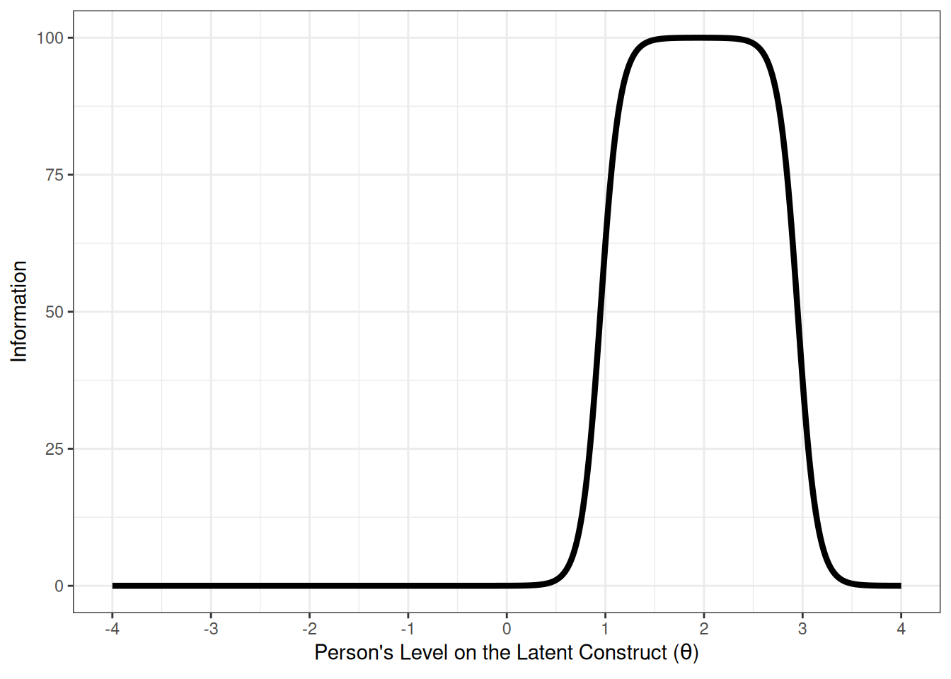
Figure 8.27: Visual Representation of a Good Measure (For Distinguishing Clinical-Range Versus Sub-Clinical Range) Based on the Test Information Curve.
8.1.8 Assumptions of IRT
IRT has several assumptions:
monotonicity
unidimensionality
item invariance
local independence
8.1.8.1 Monotonicity
The monotonicity assumption holds that a person’s probability of endorsing a higher level on the item increases as a person’s level on the latent construct increases. For instance, for each item assessing externalizing problems, as a child increases in their level of externalizing problems, they are expected to be rated with a higher level on that item. Monotonicity can be evaluated in multiple ways. For instance, monotonicity can be evaluated using visual inspection of empirical item characteristic curves. Another way to evaluate monotonicity is with Mokken scale analysis, such as using the mokken package in R.
8.1.8.2 Unidimensionality
The unidimensionality assumption holds that the items have one predominant dimension, which reflects the underlying (latent) construct. The dimensionality of a set of items can be evaluated using factor analysis. Although items that are intended to assess a given latent latent construct are expected to be unidimensional, models have been developed that allow multiple latent dimensions, as shown in Section 8.6. These multidimensional IRT models allow borrowing information from a given latent factor in the estimation of other latent factor(s) to account for the covariation.
The local independence assumptions holds that the items are uncorrelated when controlling for the latent dimension. That is, IRT models assume that the items’ errors (residuals) are uncorrelated with each other. Factor analysis and structural equation models can relax this assumption and allow items’ error terms to correlate with each other.
LSAT7 is a data set from the mirt package (Chalmers, 2020) that contains five items from the Law School Admissions Test. SAT12 is a data set from the mirt package (Chalmers, 2020) that contains 32 items for a grade 12 science assessment test (SAT) measuring topics of chemistry, biology, and physics.
A measure that is a raw symptom count (i.e., a count of how many symptoms a person endorses) is low in precision and has a high standard error of measurement. Some diagnostic measures provide an ordinal response scale for each symptom. For example, the Structured Clinical Interview of Mental Disorders (SCID) provides a response scale from 0 to 2, where 0 = the symptom is absent, 1 = the symptom is sub-threshold, and 2 = the symptom is present. If your measure was a raw symptom sum, as opposed to a count of how many symptoms were present, the measure would be slightly more precise and have a somewhat smaller standard error of measurement.
A weighted symptom sum is the classical test theory analog of IRT. In classical test theory, proportion correct (or endorsed) would correspond to item difficulty and the item–total correlation (i.e., a point-biserial correlation) would correspond to item discrimination. If we were to compute a weighted sum of each item according to its strength of association with the construct (i.e., the item–total correlation), this measure would be somewhat more precise than the raw symptom sum, but it is not a latent variable method.
In IRT analysis, the weight for each item influences the estimate of a person’s level on the construct. IRT down-weights the poorly discriminating items and up-weights the strongly discriminating items. This leads to greater precision and a lower standard error of measurement than non-latent scoring approaches.
According to Embretson (1996), many perspectives have changed because of IRT. First, according to classical test theory, longer tests are more reliable than shorter tests, as described in Section 4.5.5.5 in the chapter on reliability. However, according to IRT, shorter tests (i.e., tests with fewer items) can be more reliable than longer tests. Item selection using IRT can lead to briefer assessments that have greater reliability than longer scales. For example, adaptive tests that tailor the difficulty of the items to the ability level of the participant.
Second, in classical test theory, a score’s meaning is tied to its location in a distribution (i.e., the norm-referenced standard). In IRT, however, the people and items are calibrated on a common scale. Based on a child’s IRT-estimated ability level (i.e., level on the construct), we can have a better sense of what the child knows and does not know, because it indicates the difficulty level at which they would tend to get items correct 50% of the time; the person would likely fail items with a higher difficulty compared to this level, whereas the person would likely pass items with a lower difficulty compared to this level. Consider Binet’s distribution of ability that arranges the items from easiest to most difficult. Based on the item difficulty and content of the items and the child’s performance, we can have a better indication that a child can perform items successfully in a particular range (e.g., count to 10) but might not be able to perform more difficult items (e.g., tie their shoes). From an intervention perspective, this would allow working in the “window of opportunity” or the zone of proximal development. Thus, IRT can provide more meaningful understanding of a person’s ability compared to traditional classical test theory interpretations such as the child being at the “63rd percentile” for a child of their age, which lacks conceptual meaning.
According to Cooper & Balsis (2009), our current diagnostic system relies heavily on how many symptoms a person endorses as an index of severity, but this assumes that all symptom endorsements have the same overall weight (severity). Using IRT, we can determine the relative severity of each item (symptom)—and it is clear that some symptoms indicate more severity than others. From this analysis, a respondent can endorse fewer, more severe items, and have overall more severe psychopathology than an individual who endorses more, less severe items. Basically, not all items are equally severe—know your items!
8.4 Rasch Model (1-Parameter Logistic)
A one-parameter logistic (1PL) item response theory (IRT) model is a model fit to dichotomous data, which estimates a different difficulty (\(b\)) parameter for each item. Discrimination (\(a\)) is not estimated (i.e., it is fixed at the same value—one—across items). Rasch models were fit using the mirt package (Chalmers, 2020).
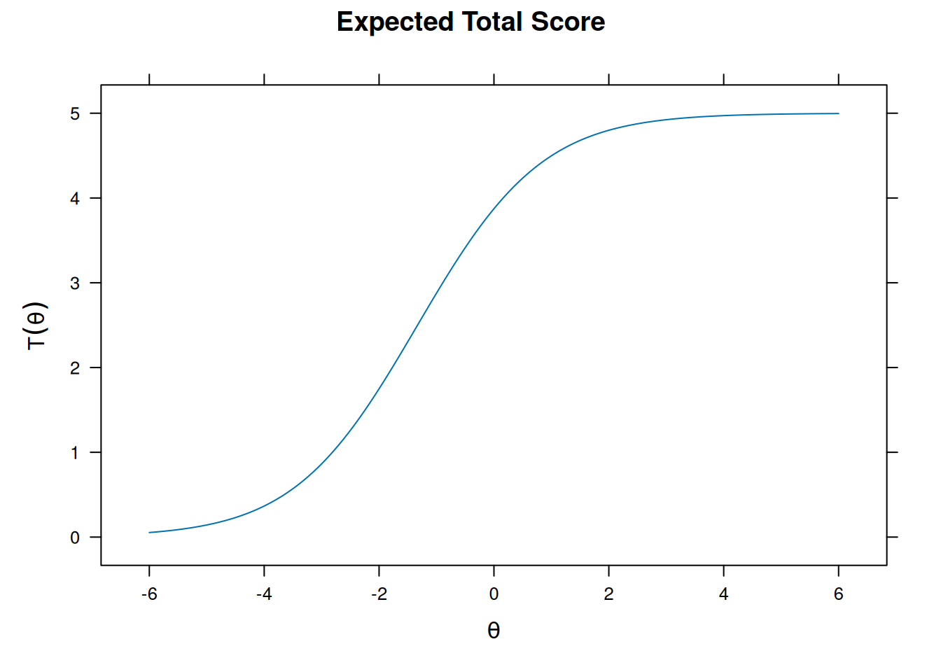
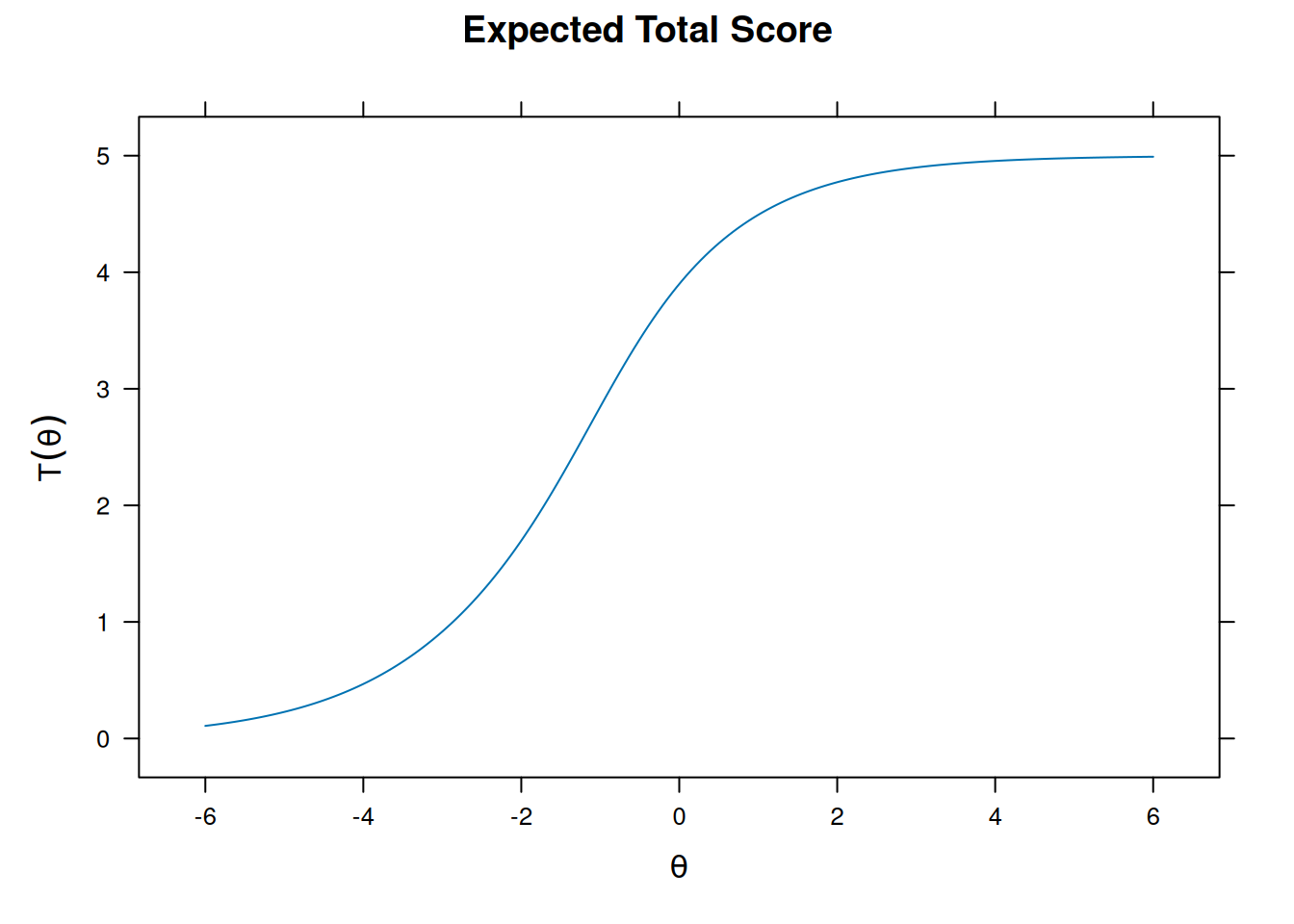
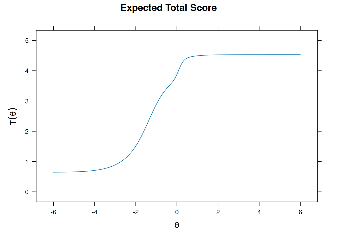
A test characteristic curve (TCC) plot of the expected total score as a function of a person’s level on the latent construct (theta; \(\theta\)) is in Figure 8.28.
Code
plot(raschModel, type ="score")
Figure 8.28: Test Characteristic Curve From Rasch Item Response Theory Model.
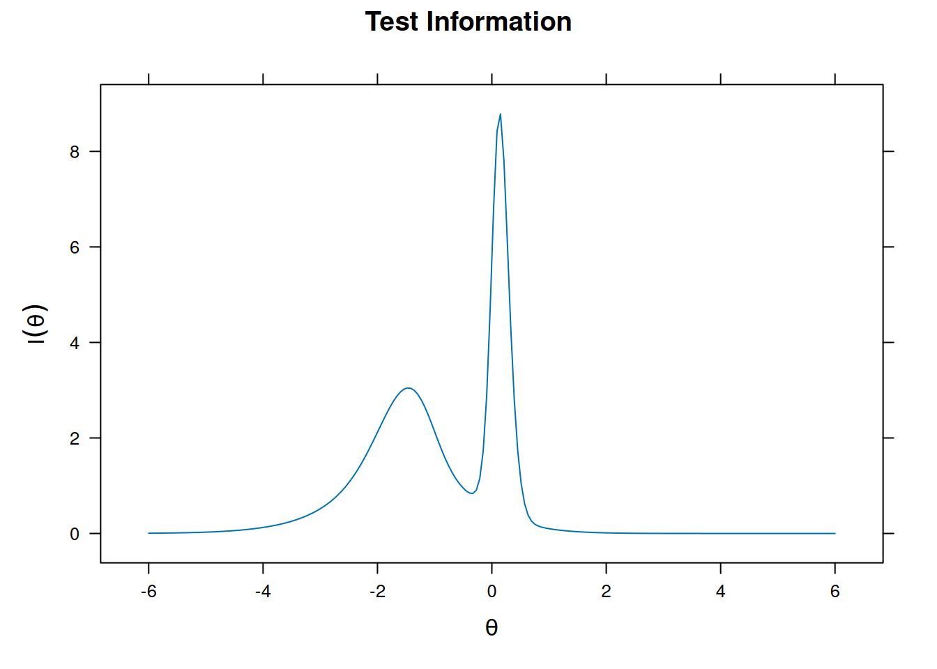
8.4.4.1.2 Test Information Curve
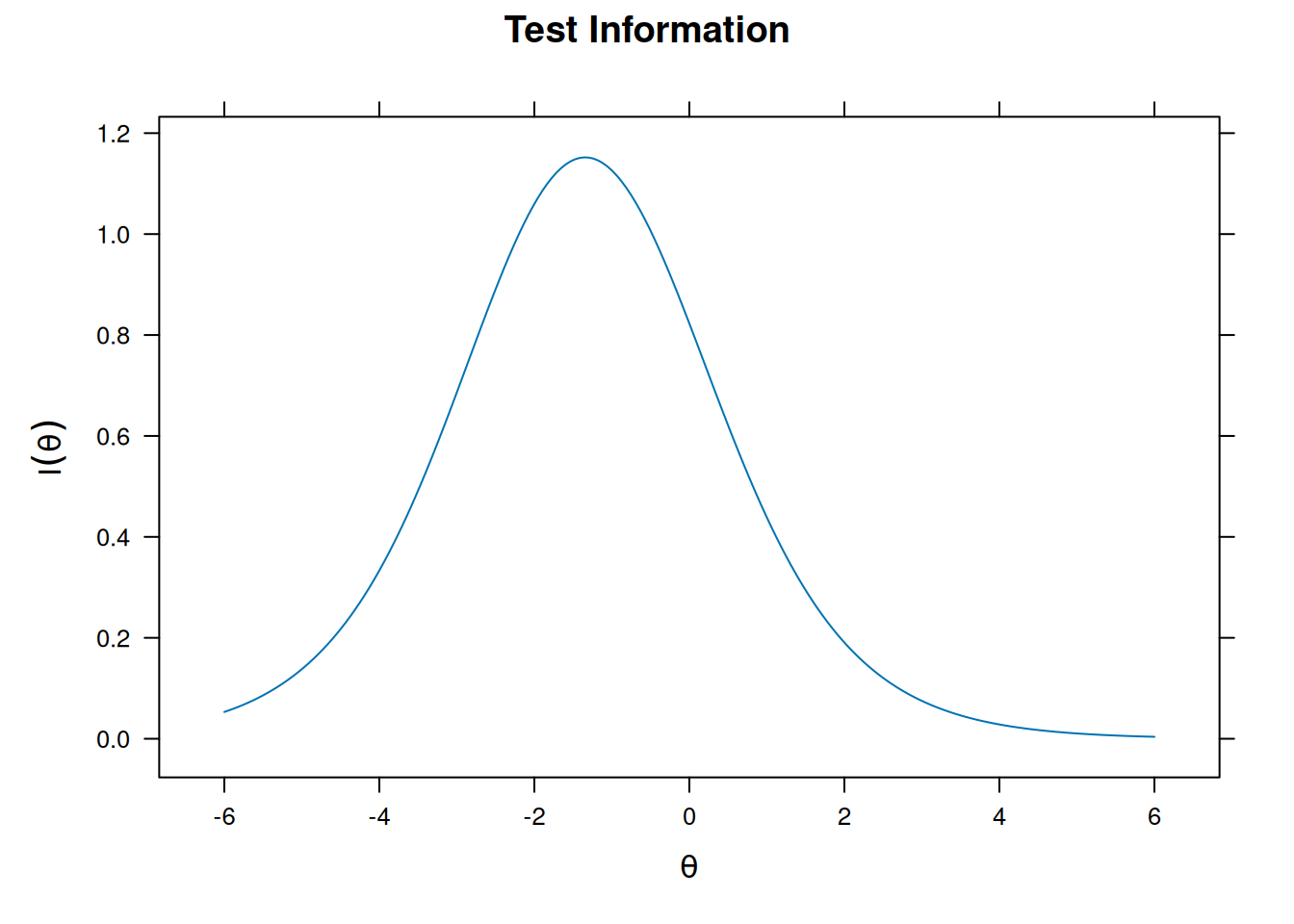
A plot of test information as a function of a person’s level on the latent construct (theta; \(\theta\)) is in Figure 8.29.
Code
plot(raschModel, type ="info")
Figure 8.29: Test Information Curve From Rasch Item Response Theory Model.
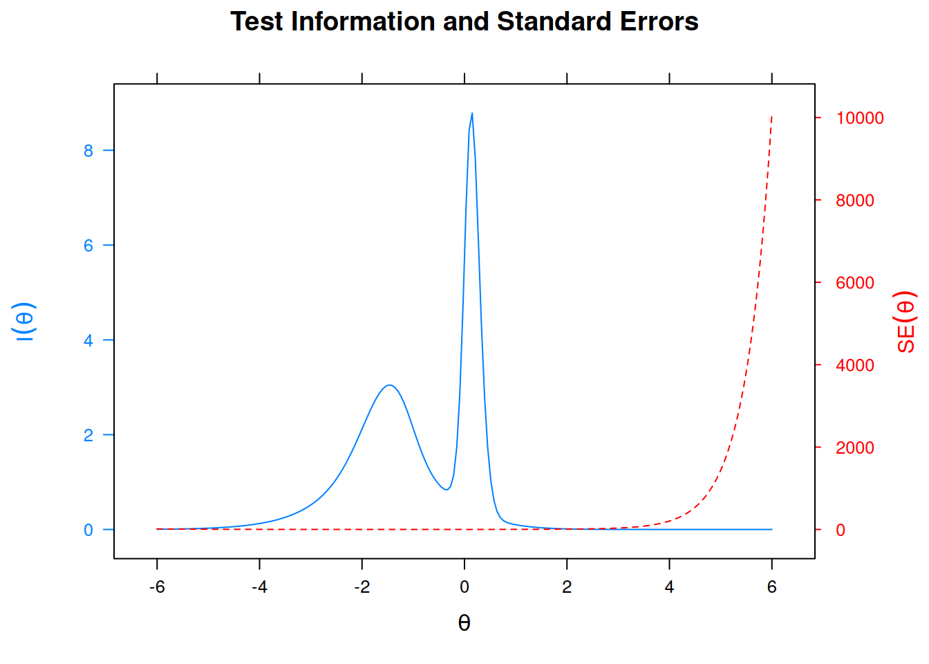
Figure 8.32: Test Information Curve and Standard Error of Measurement From Rasch Item Response Theory Model.
8.4.4.2 Item Curves
8.4.4.2.1 Item Characteristic Curves
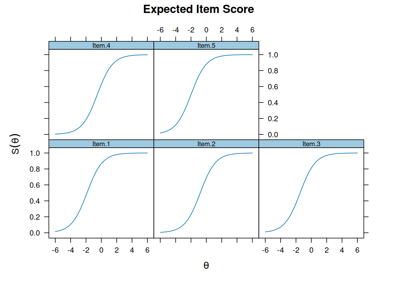
Item characteristic curve (ICC) plots of the probability of item endorsement (or getting the item correct) as a function of a person’s level on the latent construct (theta; \(\theta\)) are in Figures 8.33 and 8.34.
Code
plot(raschModel, type ="itemscore", facet_items =FALSE)
Figure 8.33: Item Characteristic Curves From Rasch Item Response Theory Model.
Code
plot(raschModel, type ="itemscore", facet_items =TRUE)
Figure 8.34: Item Characteristic Curves From Rasch Item Response Theory Model.
8.4.4.2.2 Item Information Curves
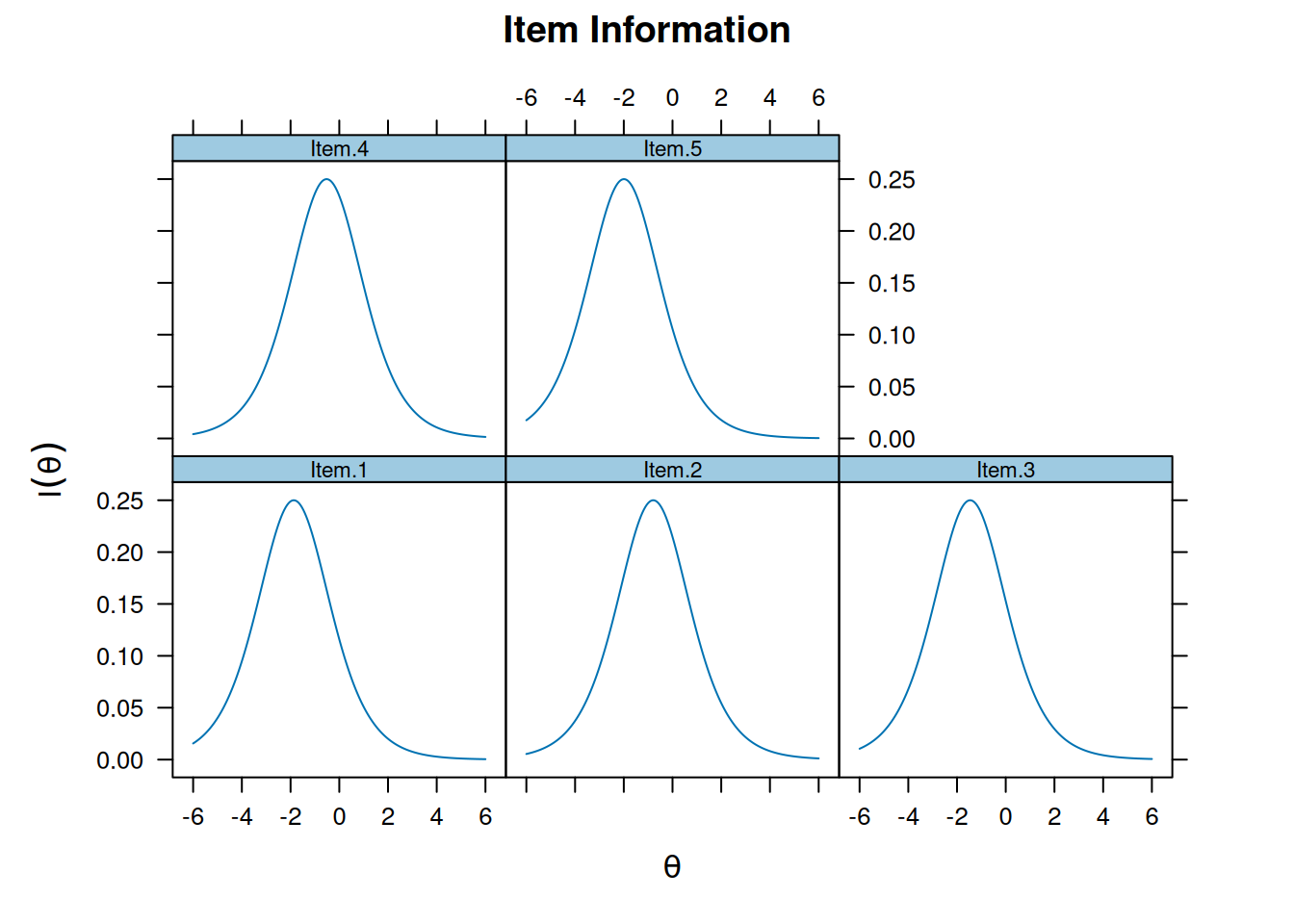
Plots of item information as a function of a person’s level on the latent construct (theta; \(\theta\)) are in Figures 8.35 and 8.36.
Code
plot(raschModel, type ="infotrace", facet_items =FALSE)
Figure 8.35: Item Information Curves from Rasch Item Response Theory Model.
Code
plot(raschModel, type ="infotrace", facet_items =TRUE)
Figure 8.36: Item Information Curves from Rasch Item Response Theory Model.
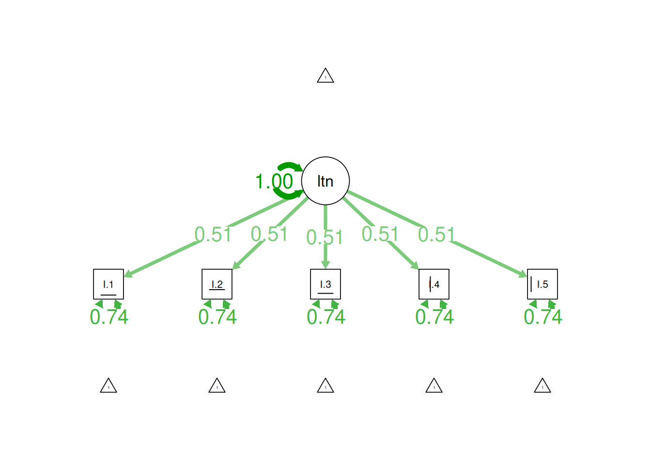
8.4.5 CFA
A one-parameter logistic model can also be fit in a CFA framework, sometimes called item factor analysis. The item factor analysis models were fit in the lavaan package (Rosseel et al., 2022).
A two-parameter logistic (2PL) IRT model is a model fit to dichotomous data, which estimates a different difficulty (\(b\)) and discrimination (\(a\)) parameter for each item. 2PL models were fit using the mirt package (Chalmers, 2020).
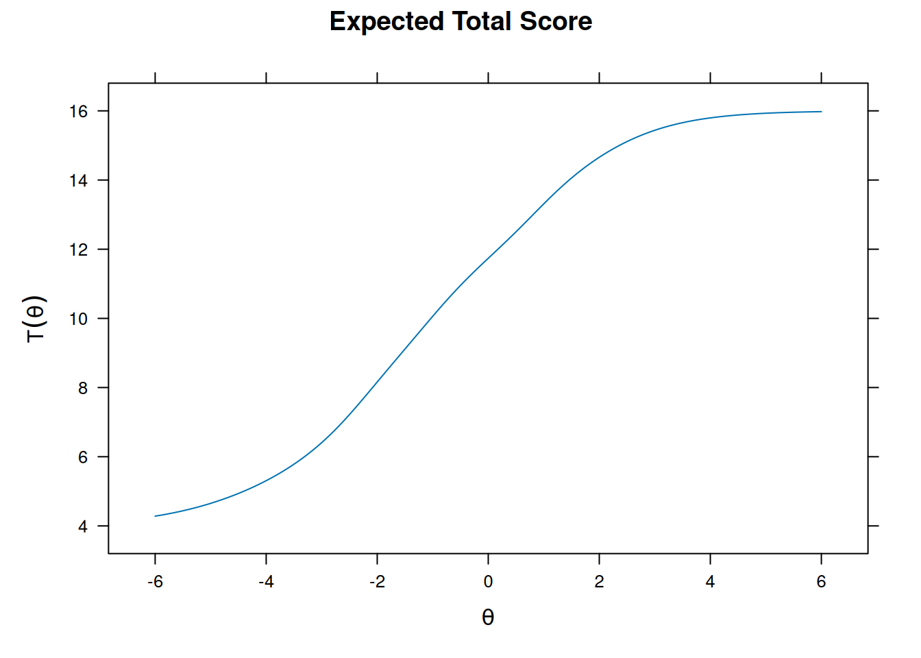
A test characteristic curve (TCC) plot of the expected total score as a function of a person’s level on the latent construct (theta; \(\theta\)) is in Figure 8.38.
Code
plot(twoPLModel, type ="score")
Figure 8.38: Test Characteristic Curve From Two-Parameter Logistic Item Response Theory Model.
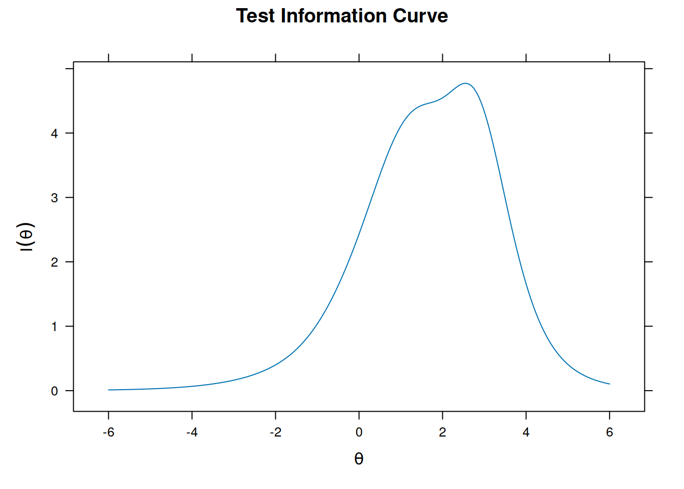
8.5.4.1.2 Test Information Curve
A plot of test information as a function of a person’s level on the latent construct (theta; \(\theta\)) is in Figure 8.39.
Code
plot(twoPLModel, type ="info")
Figure 8.39: Test Information Curve From Two-Parameter Logistic Item Response Theory Model.
Figure 8.42: Test Information Curve and Standard Error of Measurement From Two-Parameter Logistic Item Response Theory Model.
8.5.4.2 Item Curves
8.5.4.2.1 Item Characteristic Curves
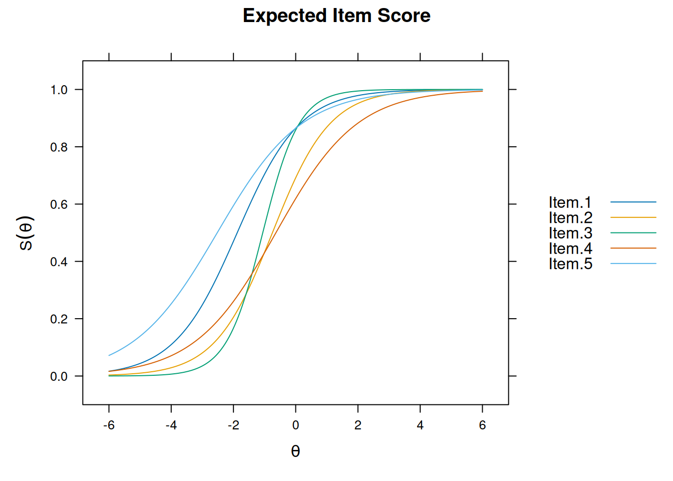
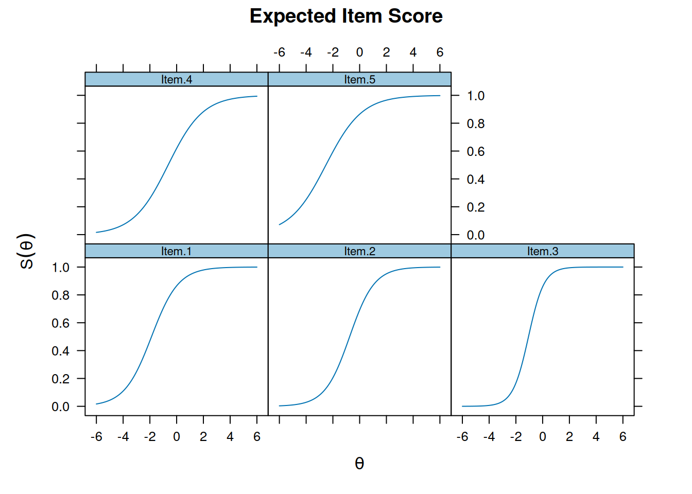
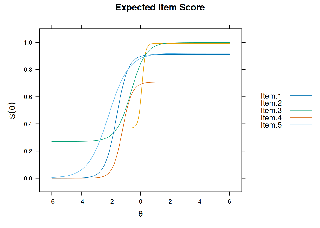
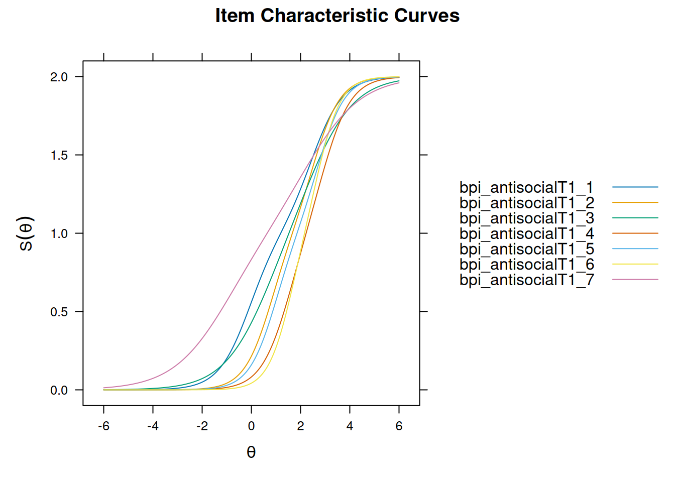
Item characteristic curve (ICC) plots of the probability of item endorsement (or getting the item correct) as a function of a person’s level on the latent construct (theta; \(\theta\)) are in Figures 8.43 and 8.44.
Code
plot(twoPLModel, type ="itemscore", facet_items =FALSE)
Figure 8.43: Item Characteristic Curves From Two-Parameter Logistic Item Response Theory Model.
Code
plot(twoPLModel, type ="itemscore", facet_items =TRUE)
Figure 8.44: Item Characteristic Curves From Two-Parameter Logistic Item Response Theory Model.
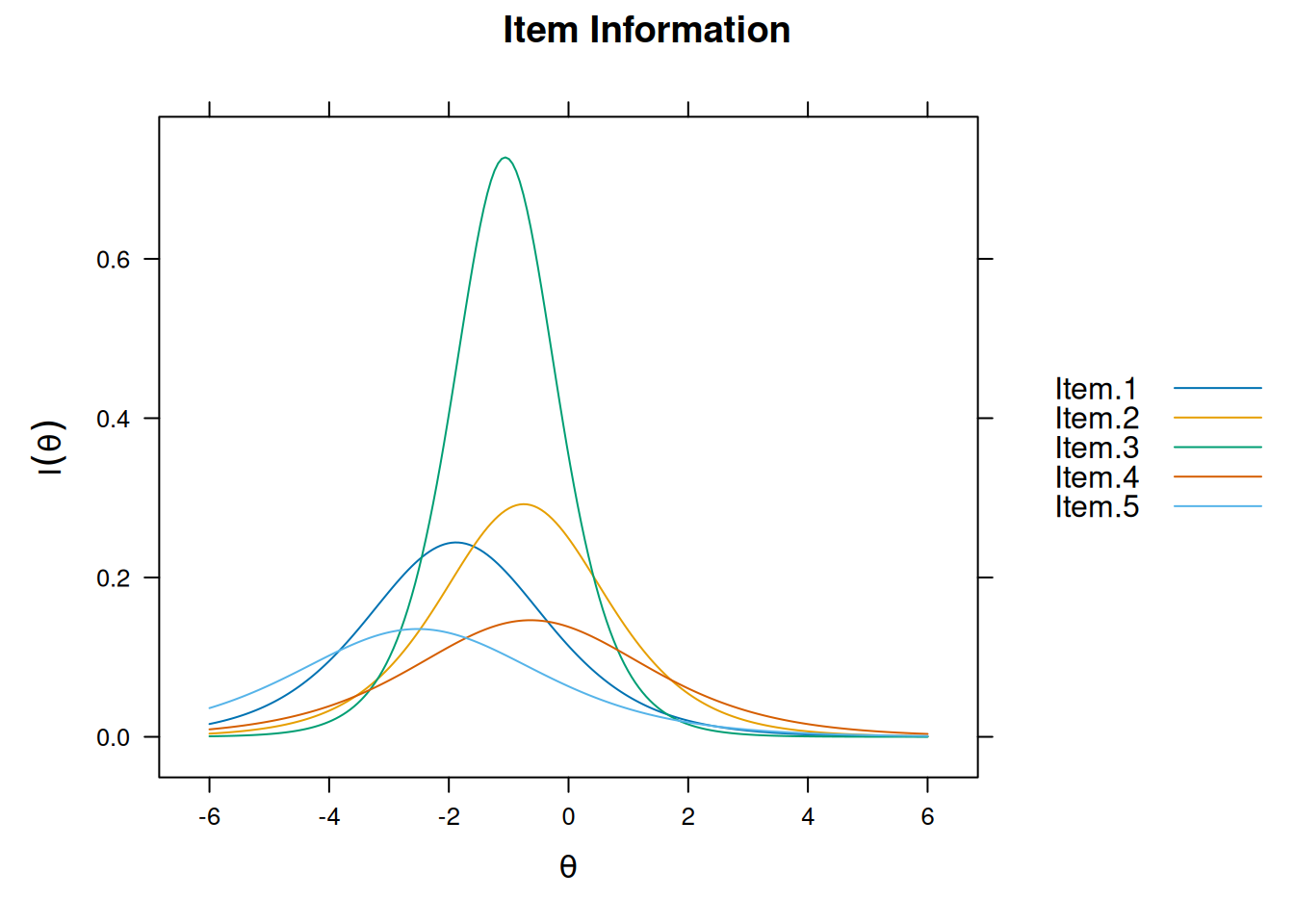
8.5.4.2.2 Item Information Curves
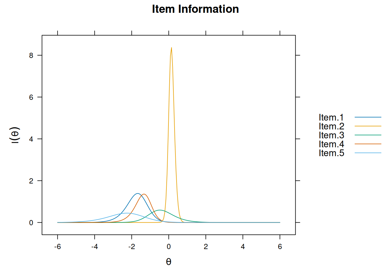
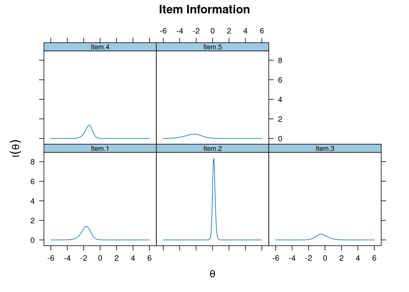
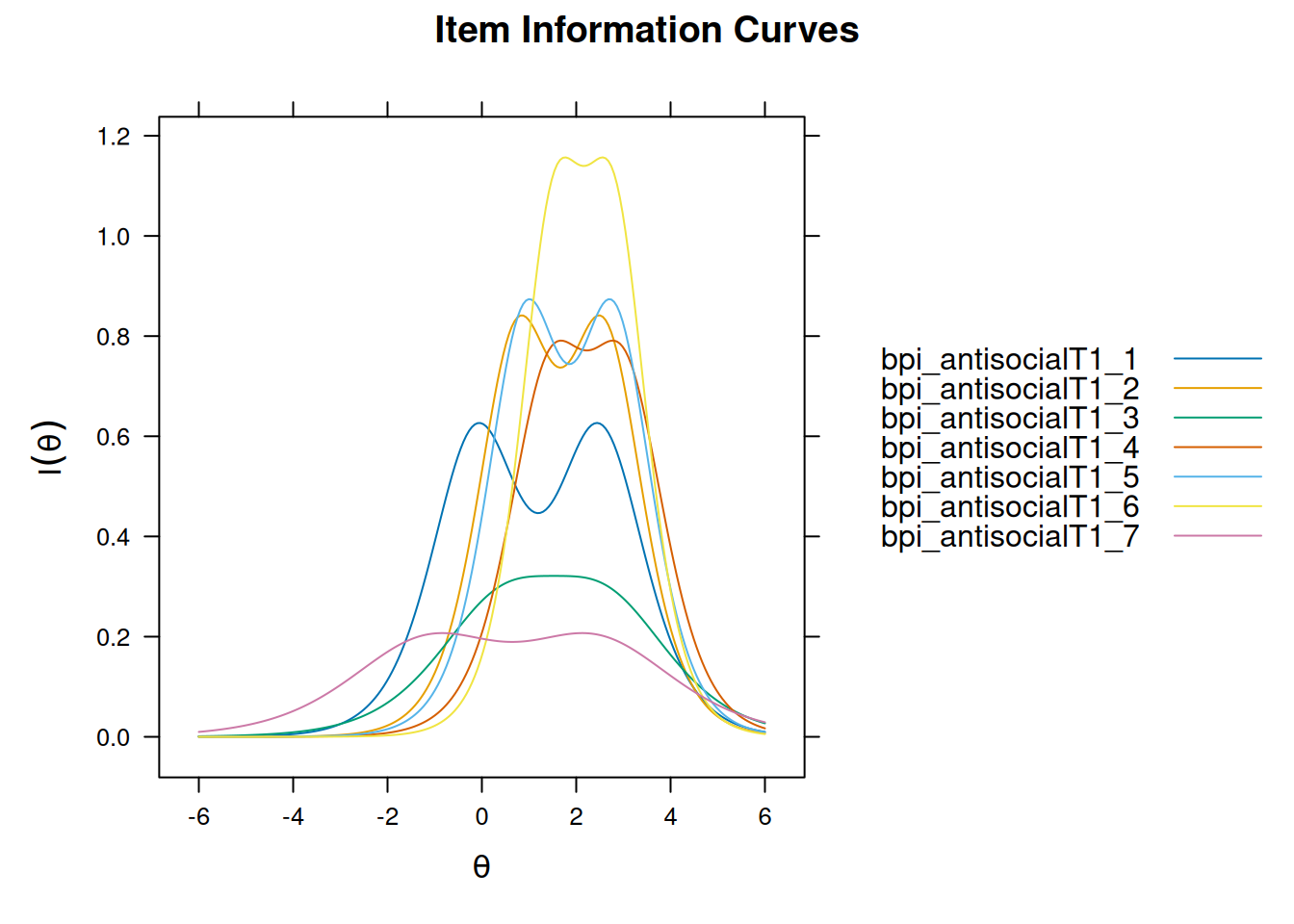
Plots of item information as a function of a person’s level on the latent construct (theta; \(\theta\)) are in Figures 8.45 and 8.46.
Code
plot(twoPLModel, type ="infotrace", facet_items =FALSE)
Figure 8.45: Item Information Curves From Two-Parameter Logistic Item Response Theory Model.
Code
plot(twoPLModel, type ="infotrace", facet_items =TRUE)
Figure 8.46: Item Information Curves From Two-Parameter Logistic Item Response Theory Model.
where \(a\) is equal to: \(\text{discrimination}/1.702\).
The petersenlab package (Petersen, 2025) contains the discriminationToFactorLoading() function that converts discrimination parameters to standardized factor loadings.
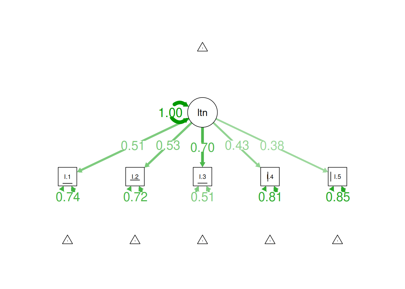
A two-parameter logistic model can also be fit in a CFA framework, sometimes called item factor analysis. The item factor analysis models were fit in the lavaan package (Rosseel et al., 2022).
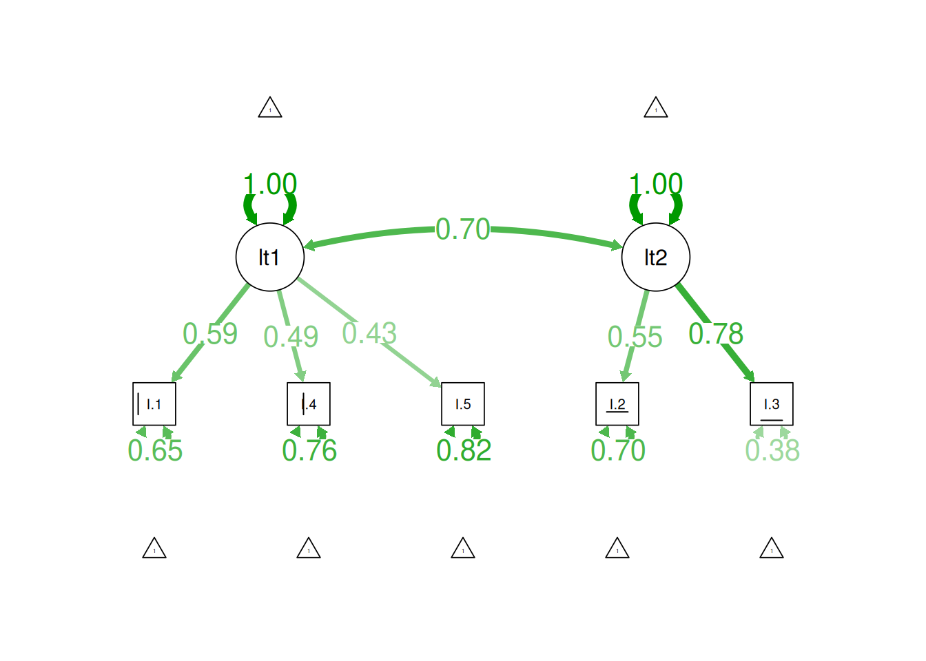
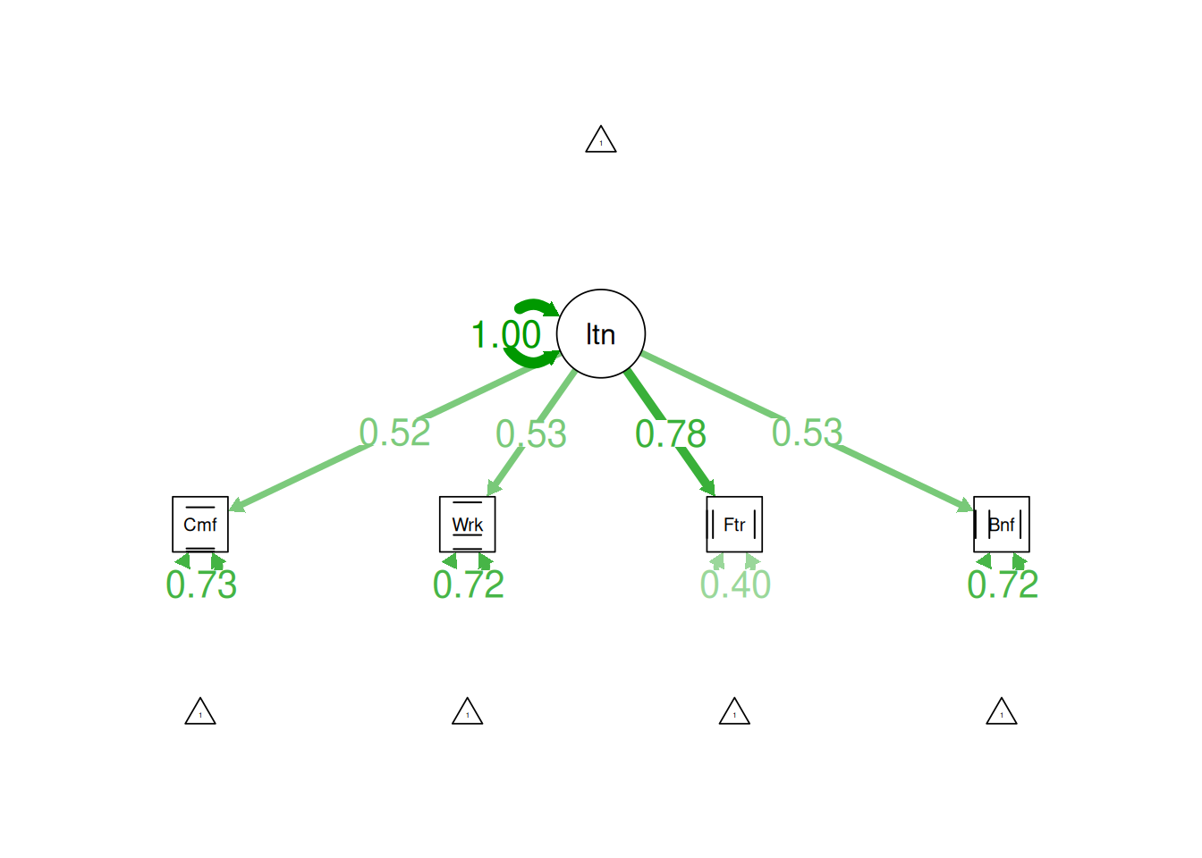
Figure 8.47: Item Factor Analysis Diagram of Two-Parameter Logistic Model.
8.6 Two-Parameter Multidimensional Logistic Model
A 2PL multidimensional IRT model is a model that allows multiple dimensions (latent factors) and is fit to dichotomous data, which estimates a different difficulty (\(b\)) and discrimination (\(a\)) parameter for each item. Multidimensional IRT models were fit using the mirt package (Chalmers, 2020). In this example, I estimate a 2PL multidimensional IRT model by estimating two factors.
The modified model with two factors and the original one-factor model are considered “nested” models. The original model is nested within the modified model because the modified model includes all of the terms of the original model along with additional terms. Model fit of nested models can be compared with a chi-square difference test.
Code
anova(twoPLModel, twoPL2FactorModel)
Using a chi-square difference test to compare two nested models, the two-factor model fits significantly better than the one-factor model.
8.6.5 Plots
8.6.5.1 Test Curves
8.6.5.1.1 Test Characteristic Curve
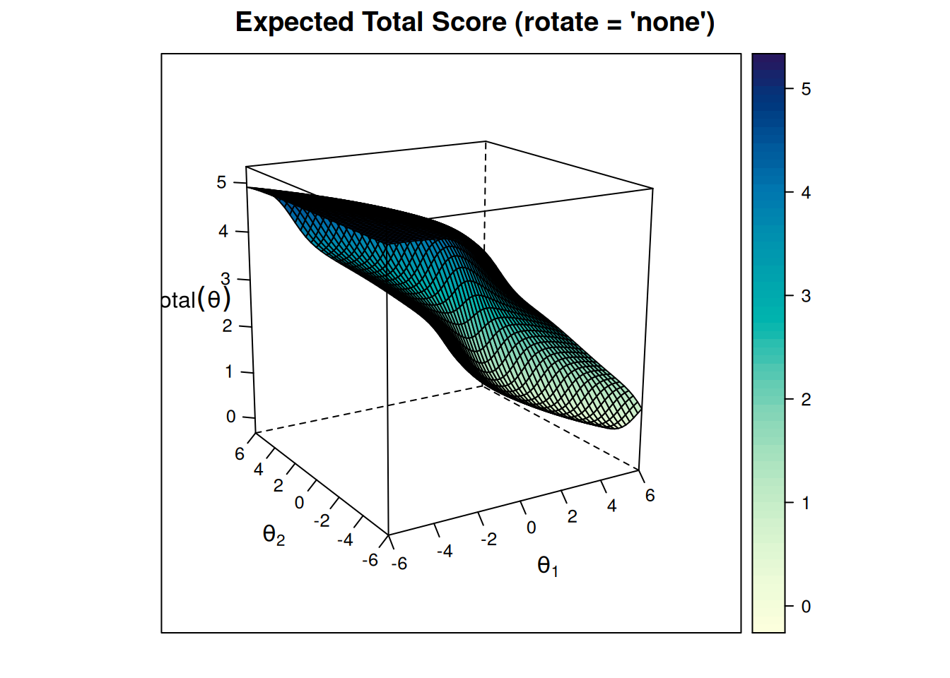
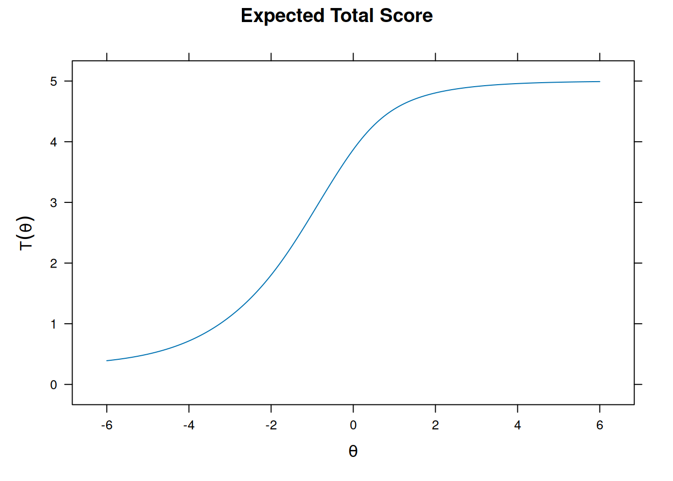
A test characteristic curve (TCC) plot of the expected total score as a function of a person’s level on each latent construct (theta; \(\theta\)) is in Figure 8.48.
Code
plot(twoPL2FactorModel, type ="score")
Figure 8.48: Test Characteristic Curve From Two-Parameter Multidimensional Item Response Theory Model.
8.6.5.1.2 Test Information Curve
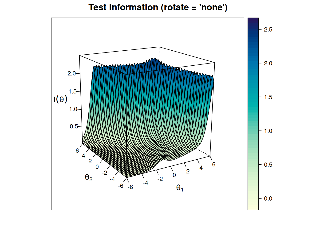
A plot of test information as a function of a person’s level on each latent construct (theta; \(\theta\)) is in Figure 8.49.
Code
plot(twoPL2FactorModel, type ="info")
Figure 8.49: Test Information Curve From Two-Parameter Multidimensional Item Response Theory Model.
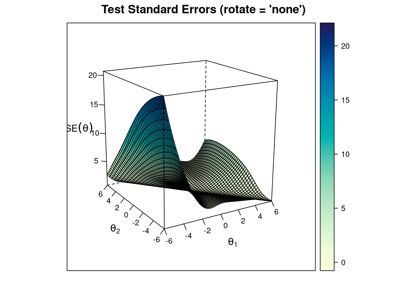
Figure 8.50: Test Standard Error of Measurement From Two-Parameter Multidimensional Item Response Theory Model.
8.6.5.2 Item Curves
8.6.5.2.1 Item Characteristic Curves
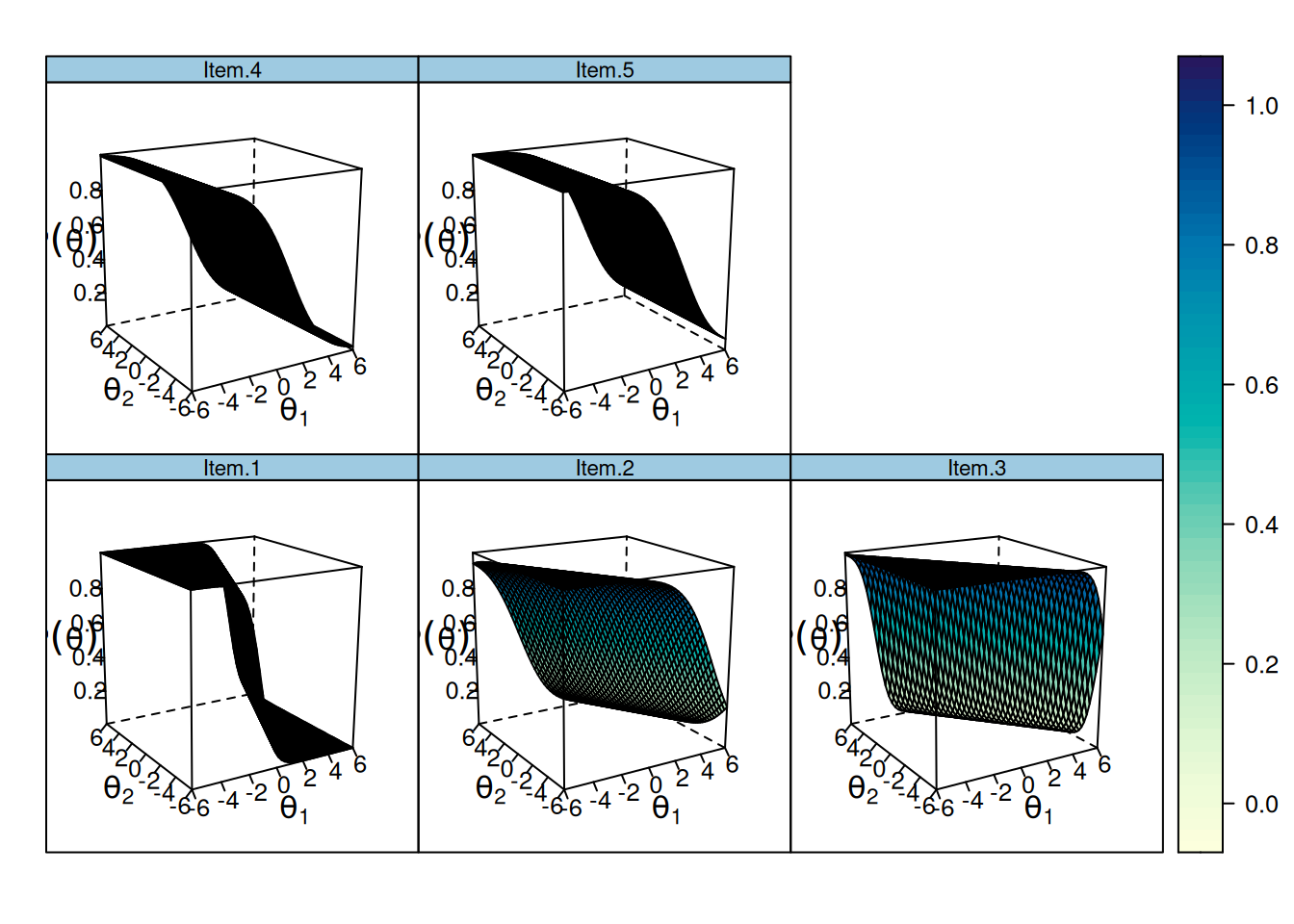
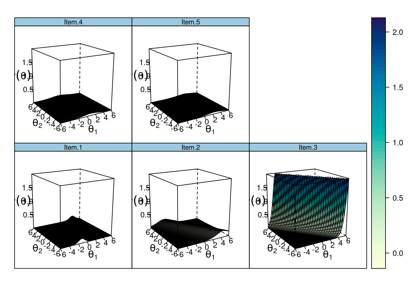
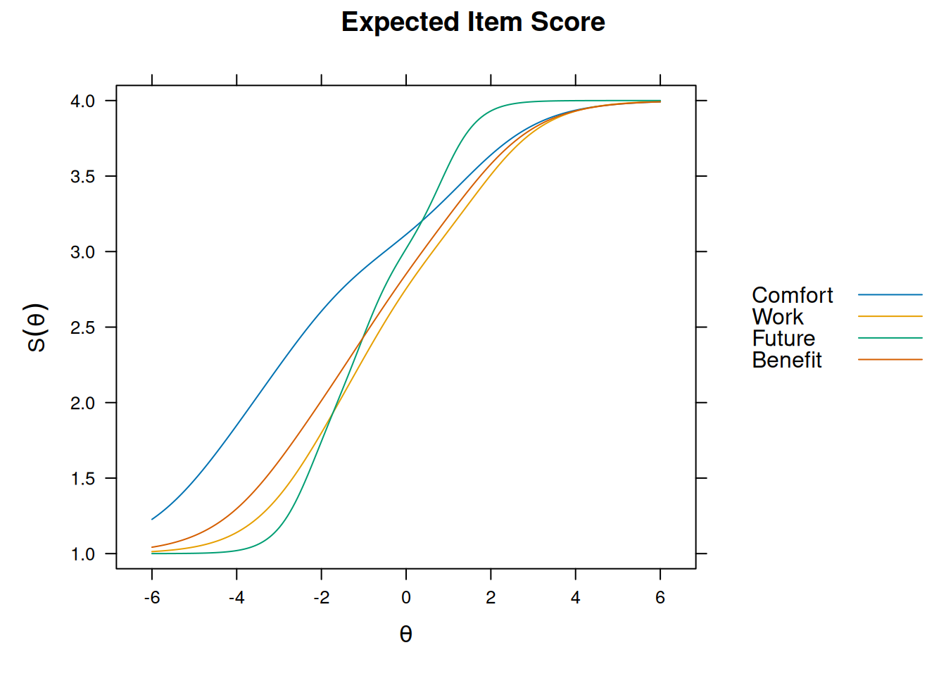
Item characteristic curve (ICC) plots of the probability of item endorsement (or getting the item correct) as a function of a person’s level on each latent construct (theta; \(\theta\)) are in Figures 8.51 and 8.52.
Code
plot(twoPL2FactorModel, type ="itemscore", facet_items =FALSE)
Figure 8.51: Item Characteristic Curves From Two-Parameter Multidimensional Item Response Theory Model.
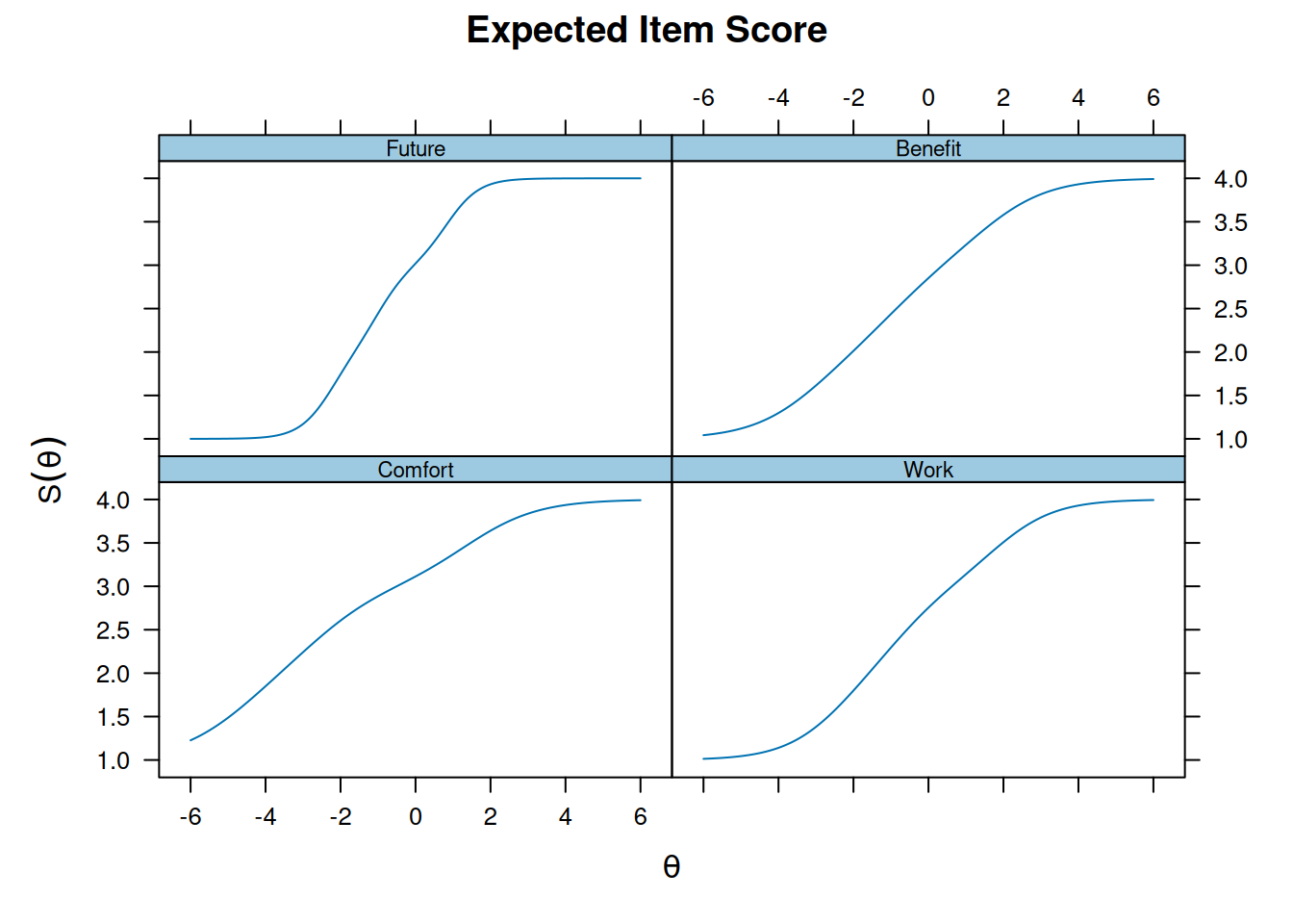
Code
plot(twoPL2FactorModel, type ="itemscore", facet_items =TRUE)
Figure 8.52: Item Characteristic Curves From Two-Parameter Multidimensional Item Response Theory Model.
8.6.5.2.2 Item Information Curves
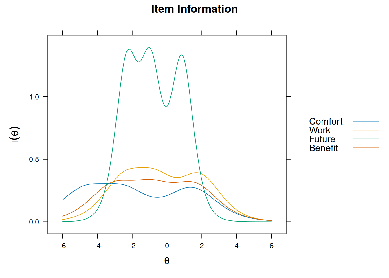
Plots of item information as a function of a person’s level on each latent construct (theta; \(\theta\)) are in Figures 8.53 and 8.54.
Code
plot(twoPL2FactorModel, type ="infotrace", facet_items =FALSE)
Figure 8.53: Item Information Curves From Two-Parameter Multidimensional Item Response Theory Model.
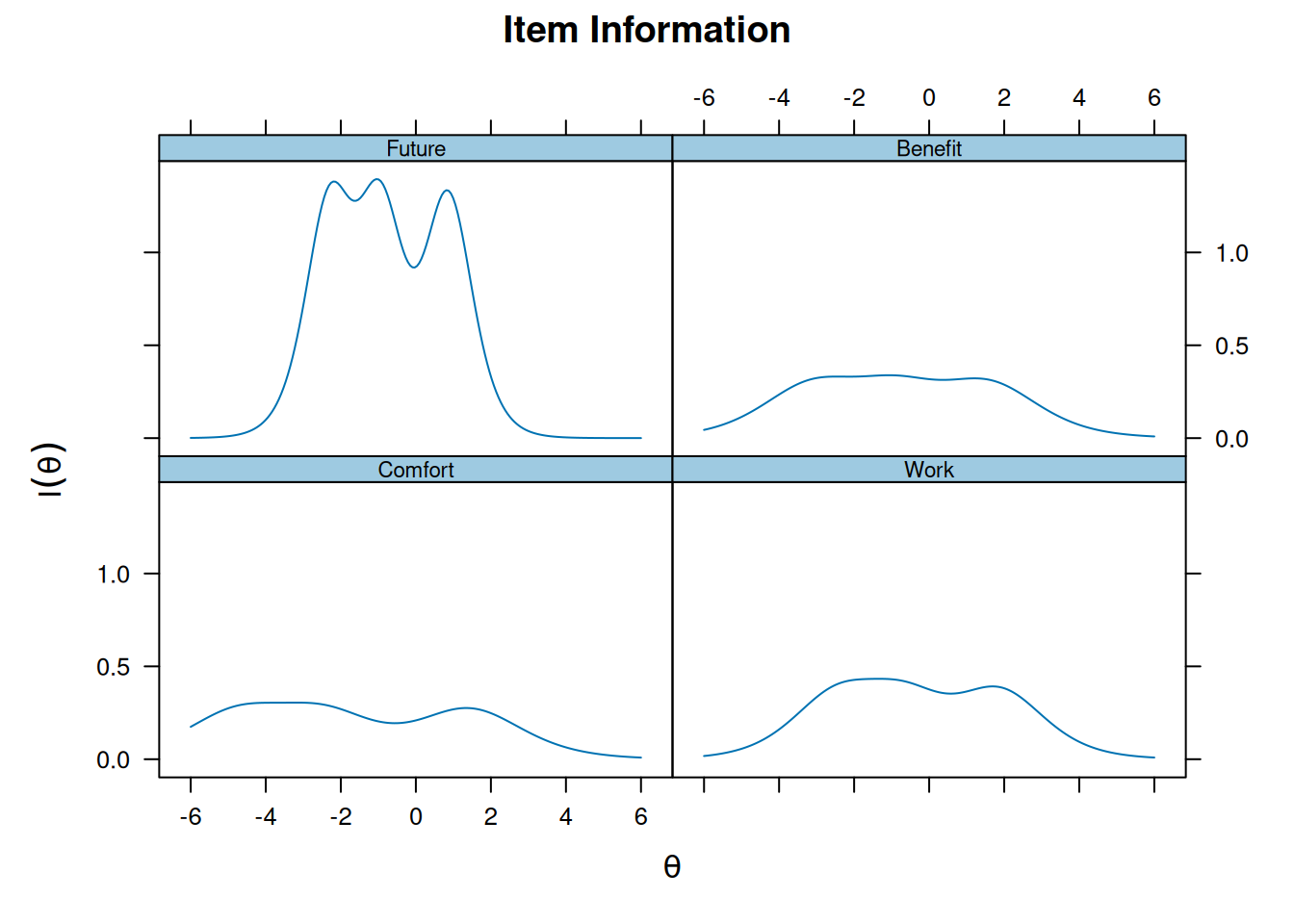
Code
plot(twoPL2FactorModel, type ="infotrace", facet_items =TRUE)
Figure 8.54: Item Information Curves From Two-Parameter Multidimensional Item Response Theory Model.
8.6.6 CFA
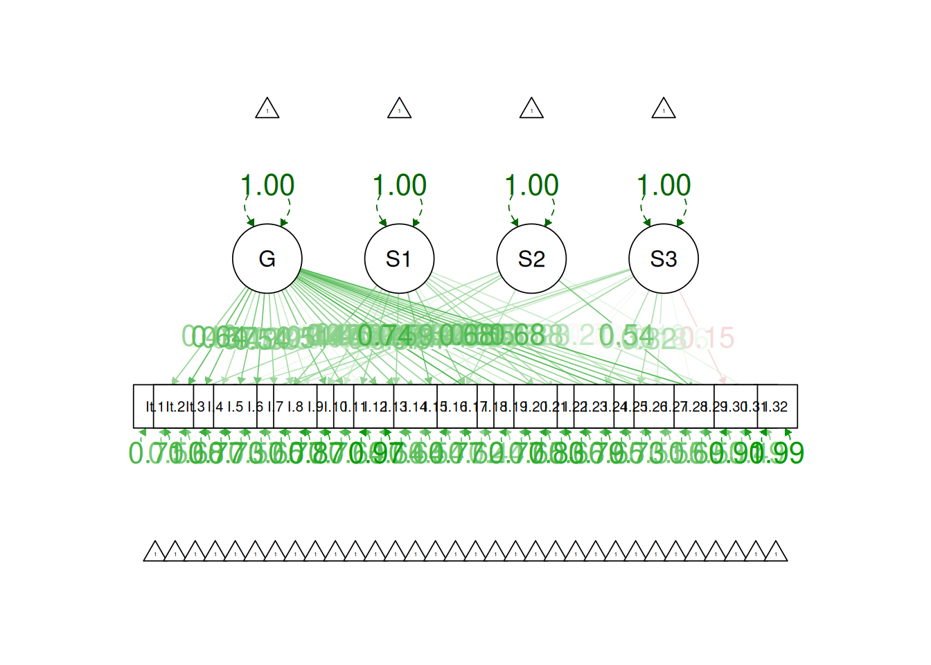
A two-parameter multidimensional model can also be fit in a CFA framework, sometimes called item factor analysis. The item factor analysis models were fit in the lavaan package (Rosseel et al., 2022).
A three-parameter logistic (3PL) IRT model is a model fit to dichotomous data, which estimates a different difficulty (\(b\)), discrimination (\(a\)), and guessing parameter for each item. 3PL models were fit using the mirt package (Chalmers, 2020).
A test characteristic curve (TCC) plot of the expected total score as a function of a person’s level on the latent construct (theta; \(\theta\)) is in Figure 8.56.
Code
plot(threePLModel, type ="score")
Figure 8.56: Test Characteristic Curve From Three-Parameter Logistic Item Response Theory Model.
8.7.4.1.2 Test Information Curve
A plot of test information as a function of a person’s level on the latent construct (theta; \(\theta\)) is in Figure 8.57.
Code
plot(threePLModel, type ="info")
Figure 8.57: Test Information Curve From Three-Parameter Logistic Item Response Theory Model.
Figure 8.60: Test Information Curve and Standard Error of Measurement From Three-Parameter Logistic Item Response Theory Model.
8.7.4.2 Item Curves
8.7.4.2.1 Item Characteristic Curves
Item characteristic curve (ICC) plots of the probability of item endorsement (or getting the item correct) as a function of a person’s level on the latent construct (theta; \(\theta\)) are in Figures 8.61 and 8.62.
Code
plot(threePLModel, type ="itemscore", facet_items =FALSE)
Figure 8.61: Item Characteristic Curves From Three-Parameter Logistic Item Response Theory Model.
Code
plot(threePLModel, type ="itemscore", facet_items =TRUE)
Figure 8.62: Item Characteristic Curves From Three-Parameter Logistic Item Response Theory Model.
8.7.4.2.2 Item Information Curves
Plots of item information as a function of a person’s level on the latent construct (theta; \(\theta\)) are in Figures 8.63 and 8.64.
Code
plot(threePLModel, type ="infotrace", facet_items =FALSE)
Figure 8.63: Item Information Curves From Three-Parameter Logistic Item Response Theory Model.
Code
plot(threePLModel, type ="infotrace", facet_items =TRUE)
Figure 8.64: Item Information Curves From Three-Parameter Logistic Item Response Theory Model.
8.8 Four-Parameter Logistic Model
A four-parameter logistic (4PL) IRT model is a model fit to dichotomous data, which estimates a different difficulty (\(b\)), discrimination (\(a\)), guessing, and careless errors parameter for each item. 4PL models were fit using the mirt package (Chalmers, 2020).
A test characteristic curve (TCC) plot of the expected total score as a function of a person’s level on the latent construct (theta; \(\theta\)) is in Figure 8.65.
Code
plot(fourPLModel, type ="score")
Figure 8.65: Test Characteristic Curve From Four-Parameter Logistic Item Response Theory Model.
8.8.4.1.2 Test Information Curve
A plot of test information as a function of a person’s level on the latent construct (theta; \(\theta\)) is in Figure 8.66.
Code
plot(fourPLModel, type ="info")
Figure 8.66: Test Information Curve From Four-Parameter Logistic Item Response Theory Model.
Figure 8.69: Test Information Curve and Standard Error of Measurement From Four-Parameter Logistic Item Response Theory Model.
8.8.4.2 Item Curves
8.8.4.2.1 Item Characteristic Curves
Item characteristic curve (ICC) plots of the probability of item endorsement (or getting the item correct) as a function of a person’s level on the latent construct (theta; \(\theta\)) are in Figures 8.70 and 8.71.
Code
plot(fourPLModel, type ="itemscore", facet_items =FALSE)
Figure 8.70: Item Characteristic Curves From Four-Parameter Logistic Item Response Theory Model.
Code
plot(fourPLModel, type ="itemscore", facet_items =TRUE)
Figure 8.71: Item Characteristic Curves From Four-Parameter Logistic Item Response Theory Model.
8.8.4.2.2 Item Information Curves
Plots of item information as a function of a person’s level on the latent construct (theta; \(\theta\)) are in Figures 8.72 and 8.73.
Code
plot(fourPLModel, type ="infotrace", facet_items =FALSE)
Figure 8.72: Item Information Curves From Four-Parameter Logistic Item Response Theory Model.
Code
plot(fourPLModel, type ="infotrace", facet_items =TRUE)
Figure 8.73: Item Information Curves From Four-Parameter Logistic Item Response Theory Model.
8.9 Graded Response Model
A two-parameter graded response model (GRM) is an IRT model fit to polytomous data (in this case, a 1–4 likert scale), which estimates a different difficulty (\(b\)) and discrimination (\(a\)) parameter for each item. It estimates four parameters for each item: difficulty [for each of three threshold transitions: 1–2 (\(b_1\)), 2–3 (\(b_2\)), and 3–4 (\(b_3\))] and discrimination (\(a\)). GRM models were fit using the mirt package (Chalmers, 2020).
8.9.1 Fit Model
Science is a data set from the mirt package (Chalmers, 2020) that contains four items evaluating people’s attitudes to science and technology on a 1–4 Likert scale. The data are from the Consumer Protection and Perceptions of Science and Technology section of the 1992 Euro-Barometer Survey of people in Great Britain.
The test curves suggest that the measure is most reliable (i.e., provides the most information and has the smallest standard error of measurement) across a wide range of construct. In general, this measure with polytomous (Likert-scale) items provides more information than the measure with binary items that were examined above. This is consistent with the idea that polytomous items tend to provide more information than binary/dichotomous items.
8.9.4.1.1 Test Characteristic Curve
A test characteristic curve (TCC) plot of the expected total score as a function of a person’s level on the latent construct (theta; \(\theta\)) is in Figure 8.74.
Code
plot(gradedResponseModel, type ="score")
Figure 8.74: Test Characteristic Curve From Graded Response Model.
8.9.4.1.2 Test Information Curve
A plot of test information as a function of a person’s level on the latent construct (theta; \(\theta\)) is in Figure 8.75.
Code
plot(gradedResponseModel, type ="info")
Figure 8.75: Test Information Curve From Graded Response Model.
Figure 8.78: Test Information Curve and Standard Error of Measurement From Graded Response Model.
8.9.4.2 Item Curves
8.9.4.2.1 Item Characteristic Curves
Item characteristic curve (ICC) plots of the expected score on the item as a function of a person’s level on the latent construct (theta; \(\theta\)) are in Figures 8.79 and 8.80.
Code
plot(gradedResponseModel, type ="itemscore", facet_items =FALSE)
Figure 8.79: Item Characteristic Curves From Graded Response Model.
Code
plot(gradedResponseModel, type ="itemscore", facet_items =TRUE)
Figure 8.80: Item Characteristic Curves From Graded Response Model.
8.9.4.2.2 Item Information Curves
Plots of item information as a function of a person’s level on the latent construct (theta; \(\theta\)) are in Figures 8.81 and 8.82.
Code
plot(gradedResponseModel, type ="infotrace", facet_items =FALSE)
Figure 8.81: Item Information Curves From Graded Response Model.
Code
plot(gradedResponseModel, type ="infotrace", facet_items =TRUE)
Figure 8.82: Item Information Curves From Graded Response Model.
A plot of the probability of item threshold endorsement as a function of a person’s level on the latent construct (theta; \(\theta\)) is in Figure 8.83.
A two-parameter graded response model can also be fit in a CFA framework, sometimes called item factor analysis. The item factor analysis models were fit in the lavaan package (Rosseel et al., 2022).
A test characteristic curve (TCC) plot of the expected total score as a function of a person’s level on the latent construct (theta; \(\theta\)) is in ?fig-bifactorTCC.
Code
plot(bifactorModel, type ="score")
8.10.5.1.2 Test Information Curve
A plot of test information as a function of a person’s level on the latent construct (theta; \(\theta\)) is in ?fig-bifactorTIF.
A plot of test reliability as a function of a person’s level on the latent construct (theta; \(\theta\)) is in ?fig-bifactorReliability.
Code
plot(bifactorModel, type ="rxx")
8.10.5.1.4 Test Standard Error of Measurement
A plot of test standard error of measurement (SEM) as a function of a person’s level on the latent construct (theta; \(\theta\)) is in ?fig-bifactorSEM.
Code
plot(bifactorModel, type ="SE")
8.10.5.1.5 Test Information Curve and Test Standard Error of Measurement
Item characteristic curve (ICC) plots of the probability of item endorsement (or getting the item correct) as a function of a person’s level on the latent construct (theta; \(\theta\)) are in Figures ?fig-bifactorICC and ?fig-bifactorICCfacet.
Code
plot(bifactorModel, type ="itemscore", facet_items =FALSE)
Code
plot(bifactorModel, type ="itemscore", facet_items =TRUE)
8.10.5.2.2 Item Information Curves
Plots of item information as a function of a person’s level on the latent construct (theta; \(\theta\)) are in Figures ?fig-bifactorIIF and ?fig-bifactorIIFfacet.
Code
plot(bifactorModel, type ="infotrace", facet_items =FALSE)
Code
plot(bifactorModel, type ="infotrace", facet_items =TRUE)
8.10.6 CFA
A bifactor model can also be fit in a CFA framework, sometimes called item factor analysis. The item factor analysis models were fit in the lavaan package (Rosseel et al., 2022).
Error in `compRelSEM()`:
! object 'isShared' not found
Code
compRelSEM(bifactorModel_cfa_fit, return.total =-1, true =list(.TOTAL. ="G")) # proportion of variance in scale composite that is attributable to general factor
Error in `compRelSEM()`:
! object 'isShared' not found
Code
AVE(bifactorModel_cfa_fit)
 G S1 S2 S3
NA NA NA NA
Code
maximalRelia(bifactorModel_cfa_fit)
Error in `calcMaximalReliaCat()`:
! The numerical method for finding the maximal reliability did not converge.
Figure 8.86: Item Factor Analysis Diagram of One-Parameter Logistic Model.
8.11 Conclusion
Item response theory is a measurement theory and advanced modeling approach that allows estimating latent variables as the common variance from multiple items, and it allows estimating how the items relate to the construct (latent variable). IRT holds promise to enable the development of briefer assessments, including short forms and adaptive assessments, that have strong reliability and validity. However, there are situations where IRT models may not be preferable, such as when assessing a formative construct, when using small sample sizes, or when assumptions of IRT are violated.
8.12 Suggested Readings
If you are interested in learning more about IRT, I highly recommend the book by Embretson & Reise (2000).
8.13 Exercises
8.13.1 Questions
Note: Several of the following questions use data from the Children of the National Longitudinal Survey of Youth Survey (CNLSY). The CNLSY is a publicly available longitudinal data set provided by the Bureau of Labor Statistics (https://www.bls.gov/nls/nlsy79-children.htm#topical-guide; archived at https://perma.cc/EH38-HDRN). The CNLSY data file for these exercises is located on the book’s page of the Open Science Framework (https://osf.io/3pwza). Children’s behavior problems were rated in 1988 (time 1: T1) and then again in 1990 (time 2: T2) on the Behavior Problems Index (BPI). Below are the items corresponding to the Antisocial subscale of the BPI:
cheats or tells lies
bullies or is cruel/mean to others
does not seem to feel sorry after misbehaving
breaks things deliberately
is disobedient at school
has trouble getting along with teachers
has sudden changes in mood or feeling
Fit a one-parameter (Rasch) model to the seven items of the Antisocial subscale of the BPI at T1. This will estimate the difficulty for each item threshold (one threshold from 0 to 1, and one threshold from 1 to 2), while constraining the discrimination for each item to be the same.
Which item has the lowest difficulty (i.e., severity) in terms of endorsing a score of one (i.e., “sometimes true”) as opposed to zero (i.e., “not true”)? Which item has the highest difficulty in terms of endorsing a score of 2 (i.e., “often true”)? What do these estimates of item difficulty indicate?
Fit a graded response model to the seven items of the Antisocial subscale of the BPI at T1. This will estimate the difficulty for each item threshold (one threshold from 0 to 1, and one threshold from 1 to 2), while allowing each item to have a different discrimination.
Provide a figure of the item characteristic curves.
Provide a figure of the item boundary characteristic curves.
Which item has the lowest discrimination? Which item has the highest discrimination? What do these estimates of item discrimination indicate?
Provide a figure of the item information curves.
Examining the item information curves, which item provides the most information at upper construct levels (2–4 standard deviations above the mean)? Which item provides the most information at lower construct levels (2–4 standard deviations below the mean)?
Provide a figure of the test information curve.
Examining the test information curve, where (at what construct levels) does the measure do the best job of assessing? Based on its information curve, describe what purposes the test would be better- or worse-suited for.
Fit a multidimensional graded response model to the seven items of the Antisocial subscale of the BPI at T1, by estimating two latent factors.
Which items loaded onto Factor 1? Which items loaded onto Factor 2? Provide a possible explanation as two why some of the items “broke off” (from Factor 1) and loaded onto a separate factor (Factor 2).
The one-factor graded response model (in #2) and the two-factor graded response model are considered “nested” models. The one-factor model is nested within the two-factor model because the two-factor model includes all of the terms of the one-factor model along with additional terms. Model fit of nested models can be directly compared with a chi-square difference test. Did the two-factor model fit better than the one-factor model?
8.13.2 Answers
Item 7 (“sudden changes in mood or feeling”) has the lowest difficulty in terms of endorsing a score of one \((b_1 = -0.95)\). Item 5 (“disobedient at school”) has the highest difficulty in terms of endorsing a score of two \((b_2 = 3.55)\). The difficulty parameter indicates the construct-level at the inflection point of the item characteristic curve. In a one- or two-parameter model, the inflection point occurs where 50% of respondents endorse the item. Thus, in this model, the difficulty parameter indicates the construct-level at which 50% of respondents endorse the item. It takes a very high level of antisocial behavior for a child to be endorsed as being often disobedient at school, whereas it does not take a high construct-level for a child to be endorsed as sometimes showing sudden changes in mood.
Below is a figure of item characteristic curves:
Code
plot(gradedResponseModel_ex, type ="itemscore", facet_items =FALSE, main ="Item Characteristic Curves")
Item 7 (“sudden changes in mood or feeling”) has the lowest discrimination \((a = 0.89)\). Item 6 (“has trouble getting along with teachers”) has the highest discrimination \((a = 2.06)\). The discrimination parameter represents the steepness of the slope of the item characteristic curve. It indicates how strongly endorsing an item discriminates (differentiates) between lower versus higher construct levels. In other words, it indicates how strongly the item is associated with the construct. Item 7 shows the weakest association with the construct, whereas item 6 shows the strongest association with the construct. That suggests that “trouble getting along with teachers” is more core to the construct of antisocial behavior than “sudden changes in mood.”
Below is a figure of item information curves:
Code
plot(gradedResponseModel_ex, type ="infotrace", facet_items =FALSE, main ="Item Information Curves")
Figure 8.89: Exercise 2c: Item Information Curves.
Item 6 (“has trouble getting along with teachers”) provides the most information at upper construct levels (2–4 standard deviations above the mean). Item 7 (“has trouble getting along with teachers”) provides the most information at lower construct levels (2–4 standard deviations below the mean). Item 1 (“cheats or tells lies”) provides the most information at somewhat low construct levels (0–2 standard deviations below the mean).
Code
plot(gradedResponseModel_ex, type ="info", main ="Test Information Curve")
Figure 8.90: Exercise 2e: Test Information Curve.
The measure does the best job of assessing (i.e., provides the most information) at construct levels from 1–3 standard deviations above the mean. Because the measure provides the most information at upper construct levels and provides little information at lower construct levels, the measure would be best used for assessing clinical versus sub-clinical levels of antisocial behavior rather than assessing individual differences in antisocial behavior across a community sample.
Items 1, 2, 3, 4, and 7 loaded onto Factor 1. Items 5 and 6 loaded onto Factor 2. Items 5 (“disobedient at school”) and 6 (“trouble getting along with teachers”) both deal with school-related antisocial behavior. Thus, the items assessing school-related antisocial behavior may share variance owing to the shared context of the behavior (school).
Yes, the two-factor model fit significantly better than the one-factor model according to a chi-square difference test \((\Delta\chi^2[df = 6.00] = 273.86, p < .001)\). Thus, antisocial behavior may not be a monolithic construct, but may depend on the context in which the behavior occurs.
Bates, D., Maechler, M., Bolker, B., & Walker, S. (2022). lme4: Linear mixed-effects models using Eigen and S4. https://github.com/lme4/lme4/
Bürkner, P.-C. (2021). Bayesian item response modeling in R with brms and Stan. Journal of Statistical Software, 100(5), 1–54. https://doi.org/10.18637/jss.v100.i05
Chen, Y., Prudêncio, R. B. C., Diethe, T., & Flach, P. (2019). \(\beta 3\)-IRT: A new item response model and its applications. arXiv:1903.04016. https://arxiv.org/abs/1903.04016
Cooper, L. D., & Balsis, S. (2009). When less is more: How fewer diagnostic criteria can indicate greater severity. Psychological Assessment, 21(3), 285–293. https://doi.org/10.1037/a0016698
Embretson, S. E., & Reise, S. P. (2000). Item response theory for psychologists (Vol. 4). Lawrence Erlbaum Associates.
Gibbons, R. D., Weiss, D. J., Frank, E., & Kupfer, D. (2016). Computerized adaptive diagnosis and testing of mental health disorders. Annual Review of Clinical Psychology, 12(1), 83–104. https://doi.org/10.1146/annurev-clinpsy-021815-093634
Krueger, R. F., Nichol, P. E., Hicks, B. M., Markon, K. E., Patrick, C. J., lacono, W. G., & McGue, M. (2004). Using latent trait modeling to conceptualize an alcohol problems continuum. Psychological Assessment, 16(2), 107–119. https://doi.org/10.1037/1040-3590.16.2.107
Rosseel, Y., Jorgensen, T. D., & Rockwood, N. (2022). lavaan: Latent variable analysis. https://lavaan.ugent.be
Smith, G. T., McCarthy, D. M., & Anderson, K. G. (2000). On the sins of short-form development. Psychological Assessment, 12(1), 102–111. https://doi.org/10.1037/1040-3590.12.1.102
Thomas, M. L. (2019). Advances in applications of item response theory to clinical assessment. Psychological Assessment, 31(12), 1442–1455. https://doi.org/10.1037/pas0000597
Feedback
Please consider providing feedback about this textbook, so that I can make it as helpful as possible. You can provide feedback at the following link:
https://forms.gle/95iW4p47cuaphTek6