I want your feedback to make the book better for you and other readers. If you find typos, errors, or places where the text may be improved, please let me know.
The best ways to provide feedback are by GitHub or hypothes.is annotations.
Alternatively, you can leave an annotation using hypothes.is.
To add an annotation, select some text and then click the
symbol on the pop-up menu.
To see the annotations of others, click the
symbol in the upper right-hand corner of the page.
3Getting Started with R for Data Analysis
The book uses the software R(R Core Team, 2025) for statistical analyses (http://www.r-project.org). R is a free software environment; you can download it at no charge here: https://cran.r-project.org. This chapter provides an overview of how to install and learn the software R, how to troubleshoot code, and how to perform various data management operations. Please note that R code is case sensitive—it treats lower case as different from upper case, so you want to be careful to use the correct case when referring to a given object.
When posting a question on forums or mailing lists, keep a few things in mind:
Read the posting guidelines before posting!
Be respectful of other people and their time. R is free software. People are offering their free time to help. They are under no obligation to help you. If you are disrespectful or act like they owe you anything, you will rub people the wrong way and will be less likely to get help.
To get started, follow the following steps (for each step that involves installing or running software, make sure to right click and select “Run as Administrator”):
After installing R and RStudio, set the executables for R and RStudio to always run with administrator permissions (so they have write access to the main installation directory for installing packages).
If on Windows, open File Explorer and find the main executable of R (C:/Program Files/R/[R-VERSION]/bin/R.exe) and RStudio (C:/Program Files/RStudio/bin/RStudio.exe). Right-click it to open the contextual menu. Then, click on “Properties”. In the Properties window, go to the Compatibility tab. At the bottom of the window, check the box next to the “Run this program as an administrator” option, and then click OK.
Open RStudio (by right clicking and selecting “Run as Administrator”).
Some necessary packages, including the ffanalytics package(Tungate et al., 2025), are hosted in GitHub (and are not hosted on the Comprehensive R Archive Network [CRAN]) and thus need to be installed using the following code (after installing the remotes package (Csárdi et al., 2024) above)1:
Click “Use this Template” (in the top right of the screen) > “Create a new repository”
Make sure the checkbox is selected for the following option: “Include all branches”
Make sure your Owner account is selected
Specify the repository name to whatever you want, such as FantasyFootballBlog
Type a brief description, such as Files for my fantasy football blog
Keep the repository public (this is necessary for generating your blog)
Select “Create repository”
After creating the new repository, make sure you are on the page of your new repository and complete the following steps:
Click “Settings” (in the top of the screen)
Click “Actions” (in the left sidebar) > “General”
Make sure the following are selected:
“Read and write permissions” (under “Workflow permissions”)
“Allow GitHub Actions to create and approve pull requests”
then click “Save”
Click “Pages” (in the left sidebar)
Make sure the following are selected:
“Deploy from a branch” (under “Source”)
“gh-pages/(root)” (under “Branch”)
then click “Save”
Clone the repository to your local computer by clicking “Code” > “Open with GitHub Desktop”, select the folder where you want the repository to be saved on your local computer, and click “Clone”
3.5 General Workflow
Here is a general workflow for statistical analysis:
Load the packages you need
Load the data files
Do any data processing needed to prepare the data files to be merged.
For example, make sure each data file has unique values on the keys.
Merge the data files
Do any data processing needed to prepare the data files for analysis. For example:
calculate/recode variables
transform wide to long or long to wide
filter to the relevant rows
examine descriptive statistics to ensure data are plausible
Do the analysis!
evaluate analysis assumptions
conduct sensitivity analyses to see extent to which findings differ using different subsets of the data, different modeling approaches/assumptions, etc.
Most of the time for data analysis is typically spent getting the data ready for data analysis, including merging, cleaning, and processing. Thus, it is important to know how to perform common steps in this workflow. Below, we describe commonly used techniques for data processing and analysis.
3.6 Install Packages
In order for you to be able to load a package (to make its functions available for use), you first must install it. You can install R packages using the utils::install.packages() function with the following syntax:
Loading a package makes its functions available for use. After you have installed a package, you can load the package using the base::library() function with the following syntax:
There are many packages available for R. A package is a collection functions. In R, functions are used to perform operations given various inputs. For example, there are functions available for performing arithmetic, manipulating data, working with text, and creating plots. The function that you would use depends on what operation you intend to perform. If there is an operation that you would like to perform, there is a good chance that someone has already developed an R function to perform it. You can often find packages that include the necessary function(s) for performing a given operation by performing a Google search. And, if a function does not already exist, you can create one, as described in Section 3.29.
A function often takes particular input(s) and produces some form of output. The name of the function is followed by parentheses; the inputs go in between the parentheses. The possible inputs that a function can accept are called “arguments”. You can learn about a particular function and its arguments by entering a question mark before the name of the function:
Code
?NAME_OF_FUNCTION()
Below, we provide examples for how to learn about and use functions and arguments, by using the base::seq() function as an example. The base::seq() function creates a sequence of numbers. To learn about the base::seq() function, which creates a sequence of numbers, you can execute the following command:
Code
?seq()
This is what the documentation shows for the base::seq() function in the Usage section:
Based on this information, we know that the base::seq() function takes the following arguments:
from
to
by
length.out
along.with
...
The arguments have default values that are used if the user does not specify values for the arguments. The default values are provided in the Usage section and are in Table 3.1:
Table 3.1: Arguments and defaults for the seq() function. Arguments with a default of NULL are not used unless a value is provided by the user.
Argument
Default Value for Argument
from
1
to
1
by
((to - from)/(length.out - 1))
length.out
NULL
along.with
NULL
What each argument represents (i.e., the meaning of from, to, by, etc.) is provided in the Arguments section of the documentation. You can specify a function and its arguments either by providing values for each argument in the order indicated by the function, or by naming its arguments. Naming arguments explicitly (rather than merely relying on order) is considered best practice because it is safer—doing so prevents you from accidentally assigning an input to the wrong argument.
Here is an example of providing values to the arguments in the order indicated by the function, to create a sequence of numbers from 1 to 9:
Code
seq(1, 9)
[1] 1 2 3 4 5 6 7 8 9
Here is an example of providing values to the arguments by naming its arguments:
Code
seq(from =1,to =9,by =1)
[1] 1 2 3 4 5 6 7 8 9
If you provide values to arguments by naming the arguments, you can reorder the arguments and get the same answer:
Code
seq(by =1,to =9,from =1)
[1] 1 2 3 4 5 6 7 8 9
There are various combinations of arguments that one could use to obtain the same result. For instance, here is code to generate a sequence from 1 to 9 by 2:
Code
seq(from =1,to =9,by =2)
[1] 1 3 5 7 9
Or, alternatively, you could specify the length of the desired sequence (5 values):
Code
seq(from =1,to =9,length.out =5)
[1] 1 3 5 7 9
If you want to generate a series with decimal values, you could specify a long desired sequence of 81 values:
Hopefully, that provides an example for how to learn about a particular function, its arguments, and how to use them.
3.9 Create a Vector
A vector is a series of elements that can be numeric or character. Character elements should be specified in quotes. A vector has one dimension (length). To create a vector, use the base::c() function to combine elements into a vector (“c” stands for combine). And, we use the assignment operator (<-) to assign the vector to an object named exampleVector, so we can access it later. Anything on the right side of an assignment operator gets assigned to the object name on the left side of the assignment operator.
Code
exampleVector <-c(40, 30, 24, 20, 18, 23, 27, 32, 26, 23, NA, 37)exampleVector2 <-c("A","B1","B2","This is a sentence.","This is another sentence.")
We can then access the contents of the object by calling its name:
Code
exampleVector
[1] 40 30 24 20 18 23 27 32 26 23 NA 37
3.10 Create a Data Frame
A data frame has two dimensions: rows and columns. Here is an example of creating a data frame using the base::data.frame() function, while using the assignment operator (<-) to assign the data frame to an object so we can access it later:
Here is how you load a .RData file using a relative path (i.e., a path relative to the working directory, where the working directory is represented by a period) using the base::load() function:
Code
load(file ="./data/nfl_players.RData")
The direction of the slashes matters—you should use forward slashes (not backslashes)! To determine where you working directory is, you can use the base::getwd() function:
The petersenlab package (Petersen, 2025) has a convenience function, petersenlab::`%ni%`, for the logical operator of determining whether an element is not in a value of another vector:
The “and” operator (&) is used to string together multiple logical operators that all must evaluate as TRUE in order for the combined evaluation to evaluate as TRUE; otherwise, the combined evaluation evaluates as FALSE.
The “or” operator (|) is used to string together multiple logical operators, any of which must evaluate as TRUE in order for the combined evaluation to evaluate as TRUE; otherwise, the combined evaluation evaluates as FALSE.
The operator, base::which(), can be used to obtain the TRUE indices of an object, which is useful for subsetting.
Code
which(players$position =="RB")
[1] 4 5
3.16 If…Else Conditions
We can use the construction, if()...else if()...else() if we want to perform conditional operations. The typical construction of if()...else if()...else() operates such that it first checks if the first if() condition is true. If the first if() condition is true, it performs the operation specified and terminates the process. If the first if() condition is not true, it checks the else if() conditions in order until one of them is true. There can be multiple else if() conditions. For the first true else if() condition, it performs the operation specified and terminates the process. If none of the else if() conditions is true, it performs the operation specified under else() and then terminates the process. The construction, if()...else if()...else() can only be used on one value at a time.
Code
player_rank <-15if(player_rank <=10){ # check this condition first tier <-1print(tier)} elseif(player_rank <=20){ # if first condition was not met, check this condition next tier <-2print(tier)} elseif(player_rank <=30){ # if first two conditions were not met, check this condition next tier <-3print(tier)} else{ # if all other conditions were not met, then do thisprint("Don't draft this player!")}
[1] 2
To apply conditional operations to a vector, we can use the base::ifelse() function.
Code
player_rank <-c(1, 10, 20, 40, 100)tier <-ifelse( player_rank <=10, # check this condition1, # assign this value if true2) # assign this value if falsetier
[1] 1 1 2 2 2
3.17 Piping
In base R, if you want to perform multiple operations, it is common to either a) nest the operations, or b) save the object at each step.
Below is an example of nested operations:
Code
length(names(nfl_players))
[1] 39
Below is an example of saving the intermediate object at each step:
Code for performing nested operations can be challenging to read. Saving the intermediate object can be a waste of time to do if you are not interested in the intermediate object, and can take up unnecessary memory and computational resources. An alternative approach is to use piping. Piping allows taking the result from one computation and sending it to the next computation, thus allowing a chain of computations without saving the intermediate object at each step.
To subset a vector, use brackets to specify the elements to keep:
Code
vector[elementsToKeep]
To subset a data frame, use brackets to specify the subset of rows and columns to keep, where the value/vector before the comma specifies the rows to keep, and the value/vector after the comma specifies the columns to keep:
Code
dataframe[rowsToKeep, columnsToKeep]
You can subset by using any of the following:
numeric indices of the elements/rows/columns to keep (or drop)
names of the rows/columns to keep (or drop)
values of TRUE and FALSE corresponding to which elements/rows/columns to keep
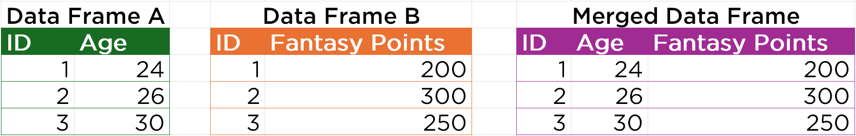
If we have two data frames that we want to combine into one we would perform what is called a merge. Let’s say we want to examine how players’ fantasy performance differs by age. Assume we have players’ age in one data frame and players’ fantasy points in a separate data frame. To examine how age and fantasy performance is related, we will need to have both variables in the same data frame. Thus, to examine age in relation to fantasy performance, we would need to merge both data frames so that the variables age and fantasy points are in the same data frame. However, to merge successfully, we need to indicate how the rows in the first data frame can be connected to the rows in the second data frame. For instance, if the player’s ID is a variable in both data frames, we could use the player’s ID as a “key” to indicate how to merge the rows from both data frames. The merged object, then, would retain the keys (i.e., player ID) and the variables from each object (i.e., age and fantasy points). An example of merge the two data frames in this example is depicted in Figure 3.1.
Merging (also called joining) merges two data objects using a shared set of variables called “keys.” The keys are the variable(s) that are used to align the rows from the two objects. The data for the given key(s) in the first object get paired with (i.e., get placed in the same row as) the data for that same key in the second object. In general, each row should have a value on each of the keys; there should be no missingness in the keys. To merge two objects, the key(s) that will be used to match the records must be present in both objects. The keys are used to merge the variables in object 1 (x) with the variables in object 2 (y). Different merge types select different rows to merge.
For some data objects, you might want to combine information for the same player from multiple data objects. If each data object is in player form (i.e., player_id uniquely identifies each row), you might merge by the player’s identification number (e.g., player_id). In this case, the key uniquely identifies each row.
However, some data objects have multiple keys. For instance, in long form data objects, each player may have multiple rows corresponding to multiple seasons. In this case, the keys may be player_id and season—that is, the data are in player-season form. If object 1 and object 2 are both in player-season form, we would use player_id and season as the keys to merge the two objects. In this case, the keys uniquely identify each row; that is, they account for the levels of nesting.
However, if the data objects are of different form, we would select the keys as the variable(s) that represent the lowest common denominator of variables used to join the data objects that are present in both objects. For instance, assume that object 1 is in player-season form. For object 2, each player has multiple rows corresponding to seasons and games/weeks—in this case, object 2 is in player-season-week form. Object 1 does not have the week variable, so it cannot be used to join the objects. Thus, we would use player_id and season as the keys to merge the two objects, because both variables are present in both objects.
It is important not to have rows with duplicate values on the keys. For instance, if there is more than one row with the same player_id in each object (or multiple rows in object 2 with the same combination of player_id, season, and week), then each row with that player_id in object 1 gets paired with each row with that player_id in object 2. The many possible combinations can lead to the resulting object greatly expanding in terms of the number of rows. Thus, you want the keys to uniquely identify each row. In the example below, player is present in each object, so we can merge by player; however, each object has multiple rows with the same player. For example, mergeExample1A has three rows for player A; mergeExample1B has two rows for player A. Thus, when we merge them, the resulting object has many more rows than each respective object (even though neither object has players that the other object does not). Below, we merge data using the dplyr::full_join() function:
Note: if the two objects include variables with the same name (apart from the keys), R will not know how you want each to appear in the merged object. So, it will add a suffix (e.g., .x, .y) to each common variable to indicate which object (i.e., object x or object y) the variable came from, where object x is the first object—i.e., the object to which object y (the second object) is merged. In general, apart from the keys, you should not include variables with the same name in two objects to be merged. To prevent this, either remove or rename the shared variable in one of the objects, or include the shared variable as a key. However, as described above, you should include it as a key only if you want to use its values to align the rows from each object. Below is an example of merging two objects with the same variable name (i.e., points) that is not used as a key, using the dplyr::full_join() function.
When two objects are merged that have different formats, the resulting data object inherits the format of the data object that has more levels of nesting. For instance, consider that you want to merge two objects, object A and object B. Object A is in player form and object B is in player-season-week form. When you merge them, the resulting data object will be in player-season-week form. Below, we merge data using the dplyr::full_join() function:
The data are structured in ID form. That is, every row in the dataset is uniquely identified by the variable, ID.
Here are the data in the fantasyPoints object:
Code
fantasyPoints
Code
dim(fantasyPoints)
[1] 4 2
3.26.3 Types of Joins
3.26.3.1 Visual Overview of Join Types
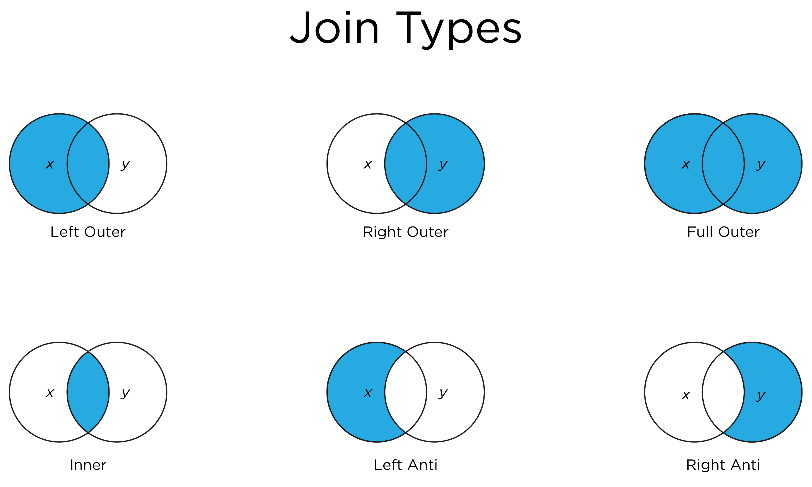
Figure 3.2 depicts various types of merges/joins. Object x is the circle labeled as x. Object y is the circle labeled as y. The area of overlap in the Venn diagram indicates the rows on the keys that are shared between the two objects (e.g., the same player_id, season, and week). The non-overlapping area indicates the rows on the keys that are unique to each object. The shaded blue area indicates which rows (on the keys) are kept in the merged object from each of the two objects, when using each of the merge types. For instance, a left outer join keeps the shared rows and the rows that are unique to object x, but it drops the rows that are unique to object y.
Figure 3.2: Types of Merges/Joins.
3.26.3.2 Full Outer Join
A full outer join includes all rows in xory. It returns columns from x and y. Here is how to merge two data frames using a full outer join (i.e., “full join”; dplyr::full_join()):
A left outer join includes all rows in x. It returns columns from x and y. Here is how to merge two data frames using a left outer join (“left join”; dplyr::left_join()):
A right outer join includes all rows in y. It returns columns from x and y. Here is how to merge two data frames using a right outer join (“right join”; dplyr::right_join()):
An inner join includes only those rows in x that have a matching record in y (i.e., the record must be in both x and y). An inner join will return that rows of x and y that have matching records, and can duplicate values of records on either side (left or right) if x and y have more than one matching record. It returns columns from x and y. Here is how to merge two data frames using an inner join (dplyr::inner_join()):
A semi join is a filter. A left semi join returns all rows from xwith a match in y. That is, it filters out records from x that are not in y. Unlike an inner join, a left semi join will never duplicate rows of x, and it includes columns from only x (not from y). Here is how to merge two data frames using a left semi join (dplyr::semi_join()):
An anti join is a filter. A left anti join returns all rows from xwithout a match in y. That is, it filters out records from x that are in y. It returns columns from only x (not from y). Here is how to merge two data frames using a left anti join (dplyr::anti_join()):
Depending on the analysis, it may be important to restructure the data to be in long or wide form. When the data are in wide form, each player has only one row. When the data are in long form, each player has multiple rows—e.g., a row for each game. The data structure is called wide or long form because a dataset in wide form has more columns and fewer rows (i.e., it appears wider and shorter), whereas a dataset in long form has more rows and fewer columns (i.e., it appears narrower and taller).
Here are the original data in long form. The data are structured in “player-season-week form”. That is, every row in the dataset is uniquely identified by the combination of variables, ID, season, and week—these are the keys. This is an example of long form, because each player has multiple rows.
Below, we transform the data from long form to wide form. The long data are in “player-season-week form”. We widen the data by two variables (season and week), using the tidyverse ecosystem of packages (Wickham et al., 2019; Wickham, 2023), so that the data are now in “player form” (where each row is uniquely identified by the ID variable) using the tidyr::pivot_wider() function:
Conversely, we can also restructure data from wide to long using the tidyr::pivot_longer() function. Here are the data in long form, after they have been transformed from wide form using the tidyverse ecosystem of packages (Wickham et al., 2019; Wickham, 2023):
If you want to perform the same computation multiple times, it can be faster to do it in a loop compared to writing out the same computation many times. For instance, here is a loop that runs from 1 to 12 (the number of players in the players object), incrementing by 1 after each iteration. The loop prints each element of a vector (i.e., the player’s name) and the loop index (i) that indicates where the loop is in terms of its iterations:
Code
for(i in1:length(players$ID)){print(paste("The loop is at index:", i, sep =" "))print(paste("My favorite player is:", players$name[i], sep =" "))}
[1] "The loop is at index: 1"
[1] "My favorite player is: Ken Cussion"
[1] "The loop is at index: 2"
[1] "My favorite player is: Ben Sacked"
[1] "The loop is at index: 3"
[1] "My favorite player is: Chuck Downfield"
[1] "The loop is at index: 4"
[1] "My favorite player is: Ron Ingback"
[1] "The loop is at index: 5"
[1] "My favorite player is: Rhonda Ball"
[1] "The loop is at index: 6"
[1] "My favorite player is: Hugo Long"
[1] "The loop is at index: 7"
[1] "My favorite player is: Lionel Scrimmage"
[1] "The loop is at index: 8"
[1] "My favorite player is: Drew Blood"
[1] "The loop is at index: 9"
[1] "My favorite player is: Chase Emdown"
[1] "The loop is at index: 10"
[1] "My favorite player is: Justin Time"
[1] "The loop is at index: 11"
[1] "My favorite player is: Spike D'Ball"
[1] "The loop is at index: 12"
[1] "My favorite player is: Isac Ulooz"
Loops are fine for basic computations, but other approaches (such as the apply() family of functions) can be even faster than loops.
3.29 Create a Function
Now, let’s put together what we have learned to create a useful function. Functions are useful if you want to perform an operation multiple times, especially if you want to be able to manipulate various settings to make slight modifications each time. Any operation that you want to perform multiple times, you can create a function to accomplish. Use of a function can save you time without needed to retype out all of the code each time. For instance, let’s say you want to convert temperature between Fahrenheit and Celsius, you could create a function to do that. In this case, our function has two arguments: temperature (in degrees) and unit of the original temperature (F for Fahrenheit or C for Celsius, where the default unit is Fahrenheit). That allows us to make the slight modification of which unit is the input temperature and to change the calculation accordingly.
Code
convert_temperature <-function(temperature, unit ="F"){ # specify the arguments and any defaultsif(unit =="F"){ # if the input temperature(s) in Fahrenheit newtemp <- (temperature -32) / (9/5) } elseif(unit =="C"){ # if the input temperature(s) in Celsius newtemp <- (temperature * (9/5)) +32 }return(newtemp) # this is what is returned by the function}
Now we can use the function to convert temperatures between Fahrenheit and Celsius. A temperature of 32°F is equal to 0°C. A temperature of 0°C is equal to 89.6°F.
Code
convert_temperature(temperature =32,unit ="F")
[1] 0
Code
convert_temperature(temperature =32,unit ="C")
[1] 89.6
We can also convert the temperature for a vector of values at once:
To comment your code, using the # sign. Anything on the line that appears after the # sign will be interpreted as a comment and will not be evaluated by R. It is important to comment your code frequently with what you are doing doing and why so that you and others know how to read it.
Code
x <-1# this line will run# this line will NOT run: x <- 2x
[1] 1
4 Conclusion
This chapter provided an overview of how to install and learn the software R, how to troubleshoot code, and how to perform various data management operations. Most of the code throughout the book that performs data management operations leverages the techniques implemented in this chapter.
4.1 Session Info
At the end of each chapter in which R code is used, I provide the session information, which describes the system and operating system the code was run on and the versions of each package. That way, if you get different results from me, you can see which session settings differ, to help with reproducibility. If you run the (all of) the exact same code as is provided in the text, in the exact same order, with the exact same setup (platform, operating system, package versions, etc.) and the exact same data, you should get the exact same answer as is in the text. That is the idea of reproducibility—getting the exact same result with the exact same inputs. Reproducibility is crucial for studies to achieve greater confidence in their findings and to ensure better replicability of findings across studies.
Corston, R., & Colman, A. M. (2000). A crash course in SPSS for Windows. Wiley-Blackwell.
Csárdi, G., Hester, J., Wickham, H., Chang, W., Morgan, M., & Tenenbaum, D. (2024). remotes: R package installation from remote repositories, including GitHub. https://doi.org/10.32614/CRAN.package.remotes
Wickham, H., Averick, M., Bryan, J., Chang, W., McGowan, L. D., François, R., Grolemund, G., Hayes, A., Henry, L., Hester, J., Kuhn, M., Pedersen, T. L., Miller, E., Bache, S. M., Müller, K., Ooms, J., Robinson, D., Seidel, D. P., Spinu, V., … Yutani, H. (2019). Welcome to the tidyverse. Journal of Open Source Software, 4(43), 1686. https://doi.org/10.21105/joss.01686
Although the petersenlab package (Petersen, 2025) is hosted on CRAN, installing from GitHub will ensure you have the latest version.↩︎
Feedback
Please consider providing feedback about this textbook, so that I can make it as helpful as possible. You can provide feedback at the following link:
https://forms.gle/LsnVKwqmS1VuxWD18
Email Notification
The online version of this book will remain open access. If you want to know when the print version of the book is for sale, enter your email below so I can let you know.