I want your feedback to make the book better for you and other readers. If you find typos, errors, or places where the text may be improved, please let me know. The best ways to provide feedback are by GitHub or hypothes.is annotations.
You can leave a comment at the bottom of the page/chapter, or open an issue or submit a pull request on GitHub: https://github.com/isaactpetersen/Fantasy-Football-Analytics-Textbook
Alternatively, you can leave an annotation using hypothes.is.
To add an annotation, select some text and then click the
symbol on the pop-up menu.
To see the annotations of others, click the
symbol in the upper right-hand corner of the page.
16 Base Rates
This chapter provides an overview of base rates and the important roles they play in prediction.
16.1 Getting Started
16.1.1 Load Packages
16.1.2 Load Data
We created the player_stats_weekly.RData and player_stats_seasonal.RData objects in Section 4.4.3.
16.2 Overview
Predicting player performance is a complex prediction task. Performance is probabilistically influenced by many processes, including processes internal to the player in addition to external processes. Moreover, people’s performance occurs in the context of a dynamic system with nonlinear, probabilistic, and cascading influences that change across time. The ever-changing system makes behavior challenging to predict. And, similar to chaos theory, one small change in the system can lead to large differences later on. Moreover, there are important factors to keep in mind when making predictions.
Let’s consider a prediction example, assuming the following probabilities:
- The probability of contracting HIV is .3%
- The probability of a positive test for HIV is 1%
- The probability of a positive test if you have HIV is 95%
What is the probability of HIV if you have a positive test?
As we will see, the probability is: \(\frac{95\% \times .3\%}{1\%} = 28.5\%\). So based on the above probabilities, if you have a positive test, the probability that you have HIV is 28.5%. Most people tend to vastly overestimate the likelihood that the person has HIV in this example. Why? Because they do not pay enough attention to the base rate (in this example, the base rate of HIV is .3%). Base rates are important to account for when making predictions and people tend to ignore them, a phenomenon called base rate neglect, which is described in Section 14.5.1.
In general, people tend to overestimate the likelihood of low base-rate events (Kahneman, 2011). That is, if the base rate of an event or condition—such as schizophrenia—is low (e.g., ~0.5%), people overestimate the likelihood that a person has schizophrenia when given specific information about the person such as their symptoms and history. As an example of people overestimating the likelihood of low base-rate events, Fox & Tversky (1998) asked National Basketball Association (NBA) fans to estimate the probability that each of 8 teams in the playoff would win the playoffs. The median sum of probability judgments for the eight teams was 240% (Fox & Tversky, 1998; Kahneman, 2011) even though, in reality, the true probabilities must sum to 100%. The base rate for a given team to win is 12.5% (i.e., 1/8), whereas people were giving each team (on average) a 30% chance (i.e., 240/8) to win. The finding suggests that people were evaluating each team individually, considering the reasons why that particular team could win, without properly accounting for the total probability (and the base rate). In addition, people tend to overweight unlikely events in their decisions (Kahneman, 2011).
People tend to make judgments based on the representativeness (i.e., similarity to a prototype, or stereotyping) and availability heuristics rather than the base rate (Kahneman, 2011). For instance, professional scouts often make judgments about players based in part on their build and look—i.e., whethey they look the part—rather than just based on their performance (Kahneman, 2011).
Another important phenomenon is that low base-rate events (i.e., unlikely events) are difficult to predict accurately. Predictions of lower base rate phenomena tend to be lower than predictions of more common phenomena. For instance, predictions of touchdowns (less common) tend to be less accurate than predictions of yardage (more common).
Teams in the NFL also tend to neglect base rates. For instance, NFL teams give too much weight to scouting evidence in deciding which players to draft, and fail to integrate such evidence with the prior probabilities of a player’s successful future performance [i.e., the base rate of success; Massey & Thaler (2013)]. “…consider how suspiciously often we hear a college prospect described as a ‘once-in-a-lifetime player’.” (Massey & Thaler, 2013, p. 1482).
In this chapter, we describe ways to account for base rates in judgments and predictions.
16.3 Issues Around Probability
16.3.1 Types of Probabilities
It is important to distinguish between different types of probabilities: marginal probabilities, joint probabilities, and conditional probabilities.
16.3.1.1 Base Rate (Marginal Probability)
The base rate is a marginal probability, which is the general probability of an event irrespective of other things. For instance, the base rate of HIV is the probability of developing HIV. In the U.S., the prevalence rate of HIV is ~0.4% of the adult population [AIDSVu (2022); archived at https://perma.cc/8GE6-GAPC].
For instance, we can consider the following marginal probabilities:
\(P(C_i)\) is the probability (i.e., base rate) of a classification, \(C\), independent of other things. A base rate is often used as the “prior probability” in a Bayesian model. In our example above, \(P(C_i)\) is the base rate (i.e., prevalence) of HIV in the population: \(P(\text{HIV}) = .3\%\). \(P(R_i)\) is the probability (base rate) of a response, \(R\), independent of other things. In the example above, \(P(R_i)\) is the base rate of a positive test for HIV: \(P(\text{positive test}) = 1\%\). The base rate of a positive test is known as the positivity rate or selection ratio.
16.3.1.2 Joint Probability
A joint probability is the probability of two (or more) events occurring simultaneously. For instance, the probability of events \(A\) and \(B\) both occurring together is \(P(A, B)\). A joint probability can be calculated using the marginal probability of each event, as in Equation 16.1:
\[ P(A, B) = P(A) \cdot P(B) \tag{16.1}\]
Conversely (and rearranging the terms for the calculation of conditional probability), a joint probability can also be calculated using the conditional probability and marginal probability, as in Equation 16.2:
\[ P(A, B) = P(A | B) \cdot P(B) \tag{16.2}\]
16.3.1.3 Conditional Probability
A conditional probability is the probability of one event occurring given the occurrence of another event. Conditional probabilities are written as: \(P(A | B)\). This is read as the probability that event \(A\) occurs given that event \(B\) occurred. For instance, we can consider the following conditional probabilities:
\(P(C | R)\) is the probability of a classification, \(C\), given a response, \(R\). In other words, \(P(C | R)\) is the probability of having HIV given a positive test: \(P(\text{HIV} | \text{positive test})\). \(P(R | C)\) is the probability of a response, \(R\), given a classification, \(C\). In the example above, \(P(R | C)\) is the probability of having a positive test given that a person has HIV: \(P(\text{positive test} | \text{HIV}) = 95\%\).
A conditional probability can be calculated using the joint probability and marginal probability (base rate), as in Equation 16.3:
\[ P(A, B) = P(A | B) \cdot P(B) \tag{16.3}\]
16.3.2 Confusion of the Inverse
A conditional probability is not the same thing as its reverse (or inverse) conditional probability. Unless the base rate of the two events (\(C\) and \(R\)) are the same, \(P(C | R) \neq P(R | C)\). However, people frequently make the mistake of thinking that two inverse conditional probabilities are the same. This mistake is known as the “confusion of the inverse”, or the “inverse fallacy”, or the “conditional probability fallacy”. The confusion of inverse probabilities is the logical error of representative thinking that leads people to assume that the probability of \(C\) given \(R\) is the same as the probability of \(R\) given C, even though this is not true. As a few examples to demonstrate the logical fallacy, if 93% of breast cancers occur in high-risk women, this does not mean that 93% of high-risk women will eventually get breast cancer. As another example, if 77% of car accidents take place within 15 miles of a driver’s home, this does not mean that you will get in an accident 77% of times you drive within 15 miles of your home.
Which car is the most frequently stolen? It is often the Honda Accord or Honda Civic—probably because they are among the most popular/commonly available cars. The probability that the car is a Honda Accord given that a car was stolen (\(p(\text{Honda Accord } | \text{ Stolen})\)) is what the media reports and what the police care about. However, that is not what buyers and car insurance companies should care about. Instead, they care about the probability that the car will be stolen given that it is a Honda Accord (\(p(\text{Stolen } | \text{ Honda Accord})\)).
Applied to fantasy football, the probability that a given player will be injured given that he is a Running Back (\(p(\text{Injured } | \text{ RB})\)) is not the same as the probability that a given player is a Running Back given that he is injured (\(p(\text{RB } | \text{ Injured})\)).
To calculate the probability of the inverse conditional, we can leverage Bayesian statistics to calculate the probability of the inverse conditional given a conditional probability (i.e., likelihood) and the marginal probabilities (base rates) of both events. Bayesian statistics is another branch of statistics and is different from frequentist statistics and null hypothesis significance testing. Bayesian statistics is based on Bayes’ theorem, which allows updating our probability estimates based on prior information (e.g., base rate) and new data.
16.3.3 Bayes’ Theorem
16.3.3.1 Standard Formulation
An alternative way of calculating a conditional probability is using the inverse conditional probability (instead of the joint probability). This is known as Bayes’ theorem. Bayes’ theorem can help us calculate a conditional probability of some classification, \(C\), given some response, \(R\), if we know the inverse conditional probability and the base rate (marginal probability) of each. Bayes’ theorem is in Equation 16.4:
\[ \begin{aligned} P(C | R) &= \frac{P(R | C) \cdot P(C_i)}{P(R_i)} \end{aligned} \tag{16.4}\]
Or, equivalently (rearranging the terms):
\[ \begin{aligned} \frac{P(C | R)}{P(R | C)} = \frac{P(C_i)}{P(R_i)} \end{aligned} \tag{16.5}\]
Or, equivalently (rearranging the terms):
\[ \begin{aligned} \frac{P(C | R)}{P(C_i)} = \frac{P(R | C)}{P(R_i)} \end{aligned} \tag{16.6}\]
More generally, Bayes’ theorem has been described as:
\[ \begin{aligned} P(H | E) &= \frac{P(E | H) \cdot P(H)}{P(E)} \\ \text{posterior probability} &= \frac{\text{likelihood} \times \text{prior probability}}{\text{model evidence}} \end{aligned} \tag{16.7}\]
where \(H\) is the hypothesis, and \(E\) is the evidence—the new information that was not used in computing the prior probability.
In Bayesian terms, the posterior probability is the conditional probability of one event occurring given another event—it is the updated probability after the evidence is considered. In this case, the posterior probability is the probability of the classification occurring (\(C\)) given the response (\(R\)). The likelihood is the inverse conditional probability—the probability of the response (\(R\)) occurring given the classification (\(C\)). The prior probability is the marginal probability of the event (i.e., the classification) occurring, before we take into account any new information. The model evidence is the marginal probability of the other event occurring—i.e., the marginal probability of seeing the evidence.
Bayes’ theorem provides the foundation for a paradigm of statistics called Bayesian statistics, which (unlike frequentist statistics) does not use p-values.
In the HIV example above, we can calculate the conditional probability of HIV given a positive test using three terms: the conditional probability of a positive test given HIV (i.e., the sensitivity of the test), the base rate of HIV, and the base rate of a positive test for HIV. The conditional probability of HIV given a positive test is in Equation 16.8:
\[ \begin{aligned} P(C | R) &= \frac{P(R | C) \cdot P(C_i)}{P(R_i)} \\ P(\text{HIV} | \text{positive test}) &= \frac{P(\text{positive test} | \text{HIV}) \cdot P(\text{HIV})}{P(\text{positive test})} \\ &= \frac{\text{sensitivity of test} \times \text{base rate of HIV}}{\text{base rate of positive test}} \\ &= \frac{95\% \times .3\%}{1\%} = \frac{.95 \times .003}{.01}\\ &= 28.5\% \end{aligned} \tag{16.8}\]
The petersenlab package (Petersen, 2025a) contains the petersenlab::pAgivenB() function that estimates the probability of one event, \(A\), given another event, \(B\).
Thus, assuming the probabilities in the example above, the conditional probability of having HIV if a person has a positive test is 28.5%. Given a positive test, chances are higher than not that the person does not have HIV.
Now let’s see what happens if the person tests positive a second time. We would revise our “prior probability” for HIV from the general prevalence in the population (0.3%) to be the “posterior probability” of HIV given a first positive test (28.5%). This is known as Bayesian updating. We would also update the “evidence” to be the marginal probability of getting a second positive test.
If we do not know a marginal probability (i.e., base rate) of an event (e.g., getting a second positive test), we can calculate a marginal probability with the law of total probability using conditional probabilities and the marginal probability of another event (e.g., having HIV). According to the law of total probability, the probability of getting a positive test is the probability that a person with HIV gets a positive test (i.e., sensitivity) times the base rate of HIV plus the probability that a person without HIV gets a positive test (i.e., false positive rate) times the base rate of not having HIV, as in Equation 16.9:
\[ \begin{aligned} P(\text{not } C_i) &= 1 - P(C_i) \\ P(R_i) &= P(R | C) \cdot P(C_i) + P(R | \text{not } C) \cdot P(\text{not } C_i) \\ 1\% &= 95\% \times .3\% + P(R | \text{not } C) \times 99.7\% \\ \end{aligned} \tag{16.9}\]
In this case, we know the marginal probability (\(P(R_i)\)), and we can use that to solve for the unknown conditional probability that reflects the false positive rate (\(P(R | \text{not } C)\)), as in Equation 16.10:
\[ \scriptsize \begin{aligned} P(R_i) &= P(R | C) \cdot P(C_i) + P(R | \text{not } C) \cdot P(\text{not } C_i) && \\ P(R_i) - [P(R | \text{not } C) \cdot P(\text{not } C_i)] &= P(R | C) \cdot P(C_i) && \text{Move } P(R | \text{not } C) \text{ to the left side} \\ - [P(R | \text{not } C) \cdot P(\text{not } C_i)] &= P(R | C) \cdot P(C_i) - P(R_i) && \text{Move } P(R_i) \text{ to the right side} \\ P(R | \text{not } C) \cdot P(\text{not } C_i) &= P(R_i) - [P(R | C) \cdot P(C_i)] && \text{Multiply by } -1 \\ P(R | \text{not } C) &= \frac{P(R_i) - [P(R | C) \cdot P(C_i)]}{P(\text{not } C_i)} && \text{Divide by } P(R | \text{not } C) \\ &= \frac{1\% - [95\% \times .3\%]}{99.7\%} = \frac{.01 - [.95 \times .003]}{.997}\\ &= .7171515\% \\ \end{aligned} \tag{16.10}\]
We can then estimate the marginal probability of the event, substititing in \(P(R | \text{not } C)\), using the law of total probability. The petersenlab package (Petersen, 2025a) contains the petersenlab::pA() function that estimates the marginal probability of one event, \(A\).
The petersenlab package (Petersen, 2025a) contains the petersenlab::pBgivenNotA() function that estimates the probability of one event, \(B\), given that another event, \(A\), did not occur.
With this conditional probability (\(P(R | \text{not } C)\)), the updated marginal probability of having HIV (\(P(C_i)\)), and the updated marginal probability of not having HIV (\(P(\text{not } C_i)\)), we can now calculate an updated estimate of the marginal probability of getting a second positive test. The probability of getting a second positive test is the probability that a person with HIV gets a second positive test (i.e., sensitivity) times the updated probability of HIV plus the probability that a person without HIV gets a second positive test (i.e., false positive rate) times the updated probability of not having HIV, as in Equation 16.11:
\[ \begin{aligned} P(R_{i}) &= P(R | C) \cdot P(C_i) + P(R | \text{not } C) \cdot P(\text{not } C_i) \\ &= 95\% \times 28.5\% + .7171515\% \times 71.5\% = .95 \times .285 + .007171515 \times .715 \\ &= 27.58776\% \end{aligned} \tag{16.11}\]
The petersenlab package (Petersen, 2025a) contains the petersenlab::pB() function that estimates the marginal probability of one event, \(B\).
We then substitute the updated marginal probability of HIV (\(P(C_i)\)) and the updated marginal probability of getting a second positive test (\(P(R_i)\)) into Bayes’ theorem to get the probability that the person has HIV if they have a second positive test (assuming the errors of each test are independent, i.e., uncorrelated), as in Equation 16.12:
\[ \begin{aligned} P(C | R) &= \frac{P(R | C) \cdot P(C_i)}{P(R_i)} \\ P(\text{HIV} | \text{a second positive test}) &= \frac{P(\text{a second positive test} | \text{HIV}) \cdot P(\text{HIV})}{P(\text{a second positive test})} \\ &= \frac{\text{sensitivity of test} \times \text{updated base rate of HIV}}{\text{updated base rate of positive test}} \\ &= \frac{95\% \times 28.5\%}{27.58776\%} \\ &= 98.14\% \end{aligned} \tag{16.12}\]
The petersenlab package (Petersen, 2025a) contains the petersenlab::pAgivenB() function that estimates the probability of one event, \(A\), given another event, \(B\).
Thus, a second positive test greatly increases the posterior probability that the person has HIV from 28.5% to over 98%.
As seen in the rearranged formula in Equation 16.5, the ratio of the conditional probabilities is equal to the ratio of the base rates. Thus, it is important to consider base rates. People have a strong tendency to ignore (or give insufficient weight to) base rates when making predictions. The failure to consider the base rate when making predictions when given specific information about a case is known as the base rate fallacy or as base rate neglect. For example, people tend to say that the probability of a rare event is more likely than it actually is given specific information.
As seen in the rearranged formula in Equation 16.6, the inverse conditional probabilities (\(P(C | R)\) and \(P(R | C)\)) are not equal unless the base rates of \(C\) and \(R\) are the same. If the base rates are not equal, we are making at least some prediction errors. If \(P(C_i) > P(R_i)\), our predictions must include some false negatives. If \(P(R_i) > P(C_i)\), our predictions must include some false positives.
16.3.3.2 Alternative Formulation
Using the law of total probability, we can substitute the calculation of the marginal probability (\(P(R_i)\)) into Bayes’ theorem to get an alternative formulation of Bayes’ theorem, as in Equation 16.13:
\[ \begin{aligned} P(C | R) &= \frac{P(R | C) \cdot P(C_i)}{P(R_i)} \\ &= \frac{P(R | C) \cdot P(C_i)}{P(R | C) \cdot P(C_i) + P(R | \text{not } C) \cdot P(\text{not } C_i)} \\ &= \frac{P(R | C) \cdot P(C_i)}{P(R | C) \cdot P(C_i) + P(R | \text{not } C) \cdot [1 - P(C_i)]} \end{aligned} \tag{16.13}\]
Instead of using marginal probability (base rate) of \(R\), as in the original formulation of Bayes’ theorem, it uses the conditional probability, \(P(R|\text{not } C)\). Thus, it uses three terms: two conditional probabilities—\(P(R|C)\) and \(P(R|\text{not } C)\)—and one marginal probability, \(P(C_i)\).
Let us see how the alternative formulation of Bayes’ theorem applies to the HIV example above. We can calculate the probability of HIV given a positive test using three terms: the conditional probability that a person with HIV gets a positive test (i.e., sensitivity), the conditional probability that a person without HIV gets a positive test (i.e., false positive rate), and the base rate of HIV. Using the \(P(R|\text{not } C)\) calculated in Equation 16.10, the conditional probability of HIV given a single positive test is in Equation 16.14:
\[ \small \begin{aligned} P(C | R) &= \frac{P(R | C) \cdot P(C_i)}{P(R | C) \cdot P(C_i) + P(R | \text{not } C) \cdot [1 - P(C_i)]} \\ &= \frac{\text{sensitivity of test} \times \text{base rate of HIV}}{\text{sensitivity of test} \times \text{base rate of HIV} + \text{false positive rate of test} \times (1 - \text{base rate of HIV})} \\ &= \frac{95\% \times .3\%}{95\% \times .3\% + .7171515\% \times (1 - .3\%)} = \frac{.95 \times .003}{.95 \times .003 + .007171515 \times (1 - .003)}\\ &= 28.5\% \end{aligned} \tag{16.14}\]
The petersenlab package (Petersen, 2025a) contains the petersenlab::pAgivenB() function that estimates the probability of one event, \(A\), given another event, \(B\).
[1] 0.285Code
[1] 0.285To calculate the conditional probability of HIV given a second positive test, we update our priors because the person has now tested positive for HIV. We update the prior probability of HIV (\(P(C_i)\)) based on the posterior probability of HIV after a positive test (\(P(C | R)\)) that we calculated above. We can calculate the conditional probability of HIV given a second positive test using three terms: the conditional probability that a person with HIV gets a positive test (i.e., sensitivity; which stays the same), the conditional probability that a person without HIV gets a positive test (i.e., false positive rate; which stays the same), and the updated marginal probability of HIV. The conditional probability of HIV given a second positive test is in Equation 16.15:
\[ \scriptsize \begin{aligned} P(C | R) &= \frac{P(R | C) \cdot P(C_i)}{P(R | C) \cdot P(C_i) + P(R | \text{not } C) \cdot [1 - P(C_i)]} \\ &= \frac{\text{sensitivity of test} \times \text{updated base rate of HIV}}{\text{sensitivity of test} \times \text{updated base rate of HIV} + \text{false positive rate of test} \times (1 - \text{updated base rate of HIV})} \\ &= \frac{95\% \times 28.5\%}{95\% \times 28.5\% + .7171515\% \times (1 - 28.5\%)} = \frac{.95 \times .285}{.95 \times .285 + .007171515 \times (1 - .285)}\\ &= 98.14\% \end{aligned} \tag{16.15}\]
The petersenlab package (Petersen, 2025a) contains the petersenlab::pAgivenB() function that estimates the probability of one event, \(A\), given another event, \(B\).
16.3.3.3 Interim Summary
In sum, the marginal probability, including the prior probability or base rate, should be weighed heavily in predictions unless there are sufficient data to indicate otherwise, i.e., to update the posterior probability based on new evidence. People tend to ignore base rates (i.e., base rate neglect). In general, people tend to a) overestimate the likelihood of low base-rate events and b) overweight low base-rate events in their decisions (Kahneman, 2011). Bayes’ theorem specifies how prior beliefs (i.e., base rate information) should be integrated with the predictive accuracy of the evidence to make predictions. It thus provides a powerful tool to anchor predictions to the base rate unless sufficient evidence changes the posterior probability (by updating the evidence and prior probability). In general, you should anchor your predictions to the base rate and adjust from there. It is also important to question the validity of the evidence (Kahneman, 2011). As noted by Kahneman (2011), if you have doubts about the quality of the evidence for a particular prediction question, keep your predictions close to the base rate, and modify them only slightly (if at all) based on the new information.
16.4 Cab Example
Below is an example:
A cab was involved in a hit-and-run accident at night. Two cab companies, the Green and the Blue, operate in the city. You are given the following data:
- 85% of the cabs in the city are Green and 15% are Blue.
- A witness identified the cab as Blue. The court tested the reliability of the witness under the circumstances that existed on the night of the accident and concluded that the witness correctly identified each one of the two colors 80% of the time and failed 20% of the time.
What is the probability that the cab involved in the accident was Blue rather than Green?
— Kahneman (2011, p. 166)
Thus, we know the following:
\[ \begin{aligned} P(\text{Blue}) &= .15 && \text{prior probability of a Blue cab}\\ P(\text{Green}) &= .85 && \text{prior probability of a Green cab}\\ P(\text{Correct}|\text{Blue}) &= .80 && \text{probability the witness correctly identifies a Blue cab}\\ P(\text{Correct}|\text{Green}) &= .80 && \text{probability the witness correctly identifies a Green cab}\\ P(\text{Incorrect}|\text{Blue}) &= .20 && \text{probability the witness incorrectly identifies a Blue cab}\\ P(\text{Incorrect}|\text{Green}) &= .20 && \text{probability the witness incorrectly identifies a Green cab}\\ \end{aligned} \tag{16.16}\]
We want to know the probability that the cab involved in the accident was Blue, given that the witness identified it as Blue (\(P(\text{Blue}|\text{Identified as Blue})\)). To estimate this probability, we can apply Bayes’ theorem to estimate the posterior probability:
\[ \begin{aligned} P(C | R) &= \frac{P(R | C) \cdot P(C_i)}{P(R_i)}\\ P(\text{Blue}|\text{Identified as Blue}) &= \frac{P(\text{Identified as Blue}|\text{Blue}) \cdot P(\text{Blue})}{P(\text{Identified as Blue})} \end{aligned} \tag{16.17}\]
We can compute the term in the denominator (\(P(\text{Identified as Blue})\)) using the law of total probability (described in Section 16.3.3).
\[ \begin{aligned} P(R_i) &= P(R | C) \cdot P(C_i) + P(R | \text{not } C) \cdot P(\text{not } C_i)\\ P(R_i) &= P(\text{Identified as Blue}|\text{Blue}) \cdot P(\text{Blue}) + P(\text{Identified as Blue}|\text{Green}) \cdot P(\text{Green})\\ 0.29 &= (.80 \times .15) + (.20 \times .85) \\ \end{aligned} \tag{16.18}\]
We can now substitute this value into the denominator of Bayes’ theorem to estimate the posterior probability:
\[ \begin{aligned} P(C | R) &= \frac{P(R | C) \cdot P(C_i)}{P(R_i)}\\ P(\text{Blue}|\text{Identified as Blue}) &= \frac{P(\text{Identified as Blue}|\text{Blue}) \cdot P(\text{Blue})}{P(\text{Identified as Blue})}\\ 0.414 &= \frac{0.80 \times 0.15}{0.29} \end{aligned} \tag{16.19}\]
Thus, there was a 41.4% probability that the car involved in the accident was Blue rather than Green. However, when faced with this problem, people tend to ignore the base rate and go with the witness (Kahneman, 2011). According to Kahneman (2011), the most frequent response to this question regarding is that there is an 80% that the car was Blue.
16.5 Nate Silver Examples
Silver (2012) provides several examples that leverage the alternative formulation of Bayes’ theorem provided in Equation 16.13 and summarized below:
\[ \begin{aligned} P(C | R) &= \frac{P(R | C) \cdot P(C_i)}{P(R | C) \cdot P(C_i) + P(R | \text{not } C) \cdot [1 - P(C_i)]} \end{aligned} \tag{16.20}\]
In each example, the formula uses three elements to calculate the probability that the hypothesis is true:
- the conditional probability the likelihood of observing the evidence, \(R\), given that the hypothesis, \(C\), is true (i.e., \(P(R|C)\); true positive rate)
- the conditional probability the likelihood of observing the evidence, \(R\), given that the hypothesis, \(C\), is false (i.e., \(P(R | \text{not } C)\); false positive rate)
- the marginal probability (base rate) of the event occurring (i.e., the prior probability of the hypothesis, \(C\), being true; \(P(C_i)\))
Thus, the formula uses the base rate, the true positive rate (sensitivity), and the false positive rate. The ratio of the true positive rate to the false positive rate is called the positive likelihood ratio, and is used in Bayesian updating.
16.5.1 Example 1: Is Your Partner Cheating on You?
Example 1: You came home and found a strange pair of underwear in your underwear drawer. What is the probability that your partner is cheating on you?
- the prior probability that your partner is cheating on you: 4%
- the conditional probability of underwear appearing given that your partner is cheating on you: 50%
- the conditional probability of underwear appearing given that your partner is not cheating on you: 5%
16.5.2 Example 2: Does a Person Have Breast Cancer?
Example 2: What is the probability that a woman in her 40s has breast cancer if she tested positive on a mammogram?
- the prior probability that she has breast cancer: 1.4%
- the conditional probability that she has a positive test given that she has breast cancer: 75%
- the conditional probability that she has a positive test given that she does not have breast cancer: 10%
16.5.3 Example 3: Was it a Terrorist Attack?
16.5.3.1 Example 3A: The First Plane Hit the World Trade Center
Example 3A: Consider the information we had on 9/11 when the first plane hit the World Trade Center. What is the probability that a terror attack occurred given that the first plane hit the World Trade Center?
- the prior probability that terrorists crash a plane into a Manhattan skyscraper: 0.005%
- the conditional probability that a plane crashes into a Manhattan skyscraper if terrorists are attacking Manhattan skyscrapers: 100%
- the conditional probability that a plane crashes into a Manhattan skyscraper if terrorists are not attacking Manhattan skyscrapers (i.e., it is an accident): 0.008%
16.5.3.2 Example 3B: The Second Plane Hit the World Trade Center
Example 3B: Now, consider that a second plane just hit the World Trade Center. What is the probability that a terror attack occurred given that a second plane hit the World Trade Center?
- the revised prior probability that terrorists crash a plane into a Manhattan skyscraper (from Example 3A): 38.46272%
- the conditional probability that a plane crashes into a Manhattan skyscraper if terrorists are attacking Manhattan skyscrapers: 100%
- the conditional probability that a plane crashes into a Manhattan skyscraper if terrorists are not attacking Manhattan skyscrapers (i.e., it is an accident): 0.008%
16.6 Base Rates Applied to Fantasy Football
Base rates are also relevant to fantasy football. Unlike yardage (e.g., passing yards, rushing yards, receiving yards), touchdowns occur relatively less frequently. Whereas a solid Wide Receiver may log 100+ receptions and 1,200+ yards in a season, they may have “only” 8–14 receiving touchdowns in a given season. As noted in Section 17.6.6, lower base-rate events—including touchdowns—are harder to predict accurately. As noted by Harris (2012): “NFL statistical projections are basically impossible to get right. (Take it from someone who helps create them for a living.) Yes, we can do a passable job with yardage totals for players who don’t suffer unexpected injuries or depth-chart pratfalls. But so much of fantasy football hinges on touchdowns, and touchdowns are impossibly difficult to predict from season to season (let alone week to week).” (archived at https://perma.cc/4QNH-J2LD). Thus, it is important not to lend too much credence to predictions of touchdowns. Focus on other things that may be more predictable (and that may be indirectly prognostic of touchdowns) such as yards, carries/targets, receptions, depth of targets, red zone carries/targets, short distance carries/targets, etc.
In Section 17.6.6, we evaluate the accuracy of predicting touchdowns versus yardage.
When dealing with numeric predictions (rather than categorical outcomes), the equivalent of the base rate is the average value. For instance, the “base rate” of fantasy points for a given position is the average number of fantasy points for that position. We could subdivide even further to identify, for instance, the “base rate” of fantasy points for the Wide Receiver at the top of the depth chart on a team.
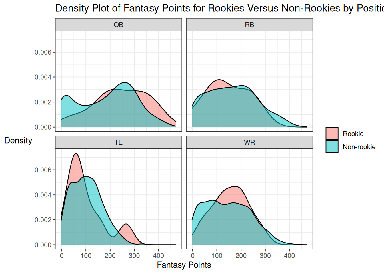
16.7 Base Rate of Rookie Performance
We examine the base rates of rookie performance compared to performance of non-rookies. It can be challenging to predict rookie performance because they have not yet played in the NFL. Thus, it is important to consider the prior probabilities (base rates) of success among rookies in the NFL. Rookies who play tend to be better players who were drafted in early rounds of the National Football League (NFL) draft. Thus, to more fairly compare rookies and non-rookies, we examine only players who were drafted in the first two rounds of the NFL Draft.
Code
rookiesDraftedEarly <- player_stats_seasonal %>%
  filter(years_of_experience == 0) %>%
  filter(draft_round %in% c(1,2)) %>%
  arrange(player_id, season) %>%
  group_by(player_id) %>%
  slice_head(n = 1) %>%
  ungroup() %>%
  mutate(
    rookie = 0,
    rookieLabel = "Rookie"
  ) %>%
  arrange(player_display_name)

nonRookiesDraftedEarly <- player_stats_seasonal %>%
  filter(years_of_experience > 0) %>%
  filter(draft_round %in% c(1,2)) %>%
  mutate(
    rookie = 1,
    rookieLabel = "Non-rookie"
  ) %>%
  arrange(player_display_name)

playersDraftedEarly <- bind_rows(
  rookiesDraftedEarly,
  nonRookiesDraftedEarly
) %>%
  mutate(rookieLabel = factor(rookieLabel, levels = c("Rookie","Non-rookie")))
Code
ggplot2::ggplot(
  data = playersDraftedEarly %>% filter(position %in% c("QB","RB","WR","TE")),
  aes(
    x = fantasyPoints)) +
  geom_density(
    aes(
      fill = rookieLabel),
    alpha = 0.5) +
  facet_wrap( ~ position) +
  labs(
    x = "Fantasy Points",
    y = "Density",
    title = "Density Plot of Fantasy Points for Rookies Versus Non-Rookies by Position"
  ) +
  theme_bw() +
  theme(
    axis.title.y = element_text(angle = 0, vjust = 0.5), # horizontal y-axis title
legend.title = element_blank()) # remove legend title16.7.1 Quarterbacks
Code
Code
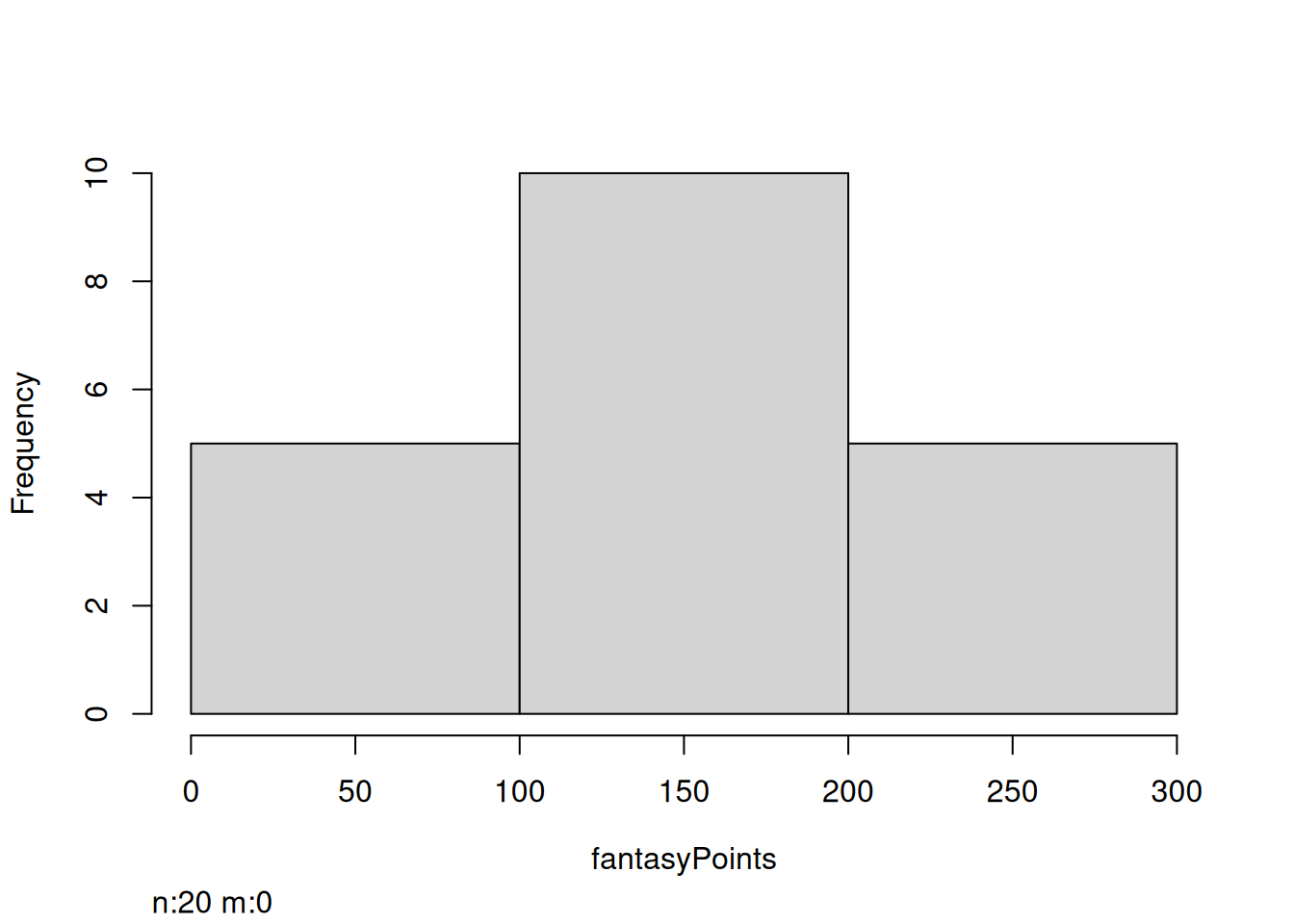
Among Quarterbacks who played a full season:
Code
16.7.2 Running Backs
Code
Code
Code
Among Running Backs who played a full season:
Code
Code
16.7.3 Wide Receivers
Code
Code
Code
Code
Among Wide Receivers who played a full season:
Code
Code
16.7.4 Tight Ends
Code
Code
Code
Code
Among Tight Ends who played a full season:
Code
Code
16.8 How to Account for Base Rates
There are various ways to account for base rates, including the use of actuarial formulas and the use of Bayesian updating.
16.8.1 Actuarial Formula
One approach to account for base rates is to use actuarial formulas (rather than human judgment) to make the predictions. Actuarial formulas based on multiple regression or machine learning can account for the base rate of the event.
16.8.2 Bayesian Updating
Another approach to account for base rates is to leverage Bayes’ theorem, using Bayesian updating and the probability nomogram. Bayesian updating is a form of anchoring and adjustment; however, unlike the anchoring and adjustment heuristic, it is a systematic approach to anchoring and adjustment that anchors one’s predictions to the base rate, and then adjusts according to new information. That is, we start with a pretest probability (i.e., base rate) and update our predictions based on the extent of new information (i.e., the likelihood ratio).
Bayesian updating can also be applied to continuous outcomes like fantasy points. For an example of applying Bayesian updating to fantasy points, see Braun (2012) (archived at https://web.archive.org/web/20161028142225/http://www.bayesff.com/bayesian101/). Applying Bayes’ theorem to continuous outcomes, the posterior distribution is equal to the prior distribution times the likelihood (data). For instance, we can start with our prior belief (distribution) for a player’s performance based on, for example, average draft position. Then, we observe the Week 1 performance. For instance, if Tom Brady scores 35 points in Week 1, our likelihood represents the likelihood that Tom Brady would score 35 points (the data). Using Bayesian updating, we can then calculate a posterior distribution that represents our new best prediction moving forward for how many points Tom Brady will score in Week 2. We then observe Week 2, generate a new likelihood and posterior distribution, and use that as our new prior distribution for Week 3, and so on. To keep things simple, we use a binary outcome below to demonstrate Bayesian updating.
To perform Bayesian updating involves comparing the relative probability of two outcomes, \(P(C | R)\) versus \(P(\text{not } C | R)\). If we want to compare the relative probability of two outcomes, we can use the odds form of Bayes’ theorem, as in Equation 16.21:
\[ \begin{aligned} P(C | R) &= \frac{P(R | C) \cdot P(C_i)}{P(R_i)} \\ P(\text{not } C | R) &= \frac{P(R | \text{not } C) \cdot P(\text{not } C_i)}{P(R_i)} \\ \frac{P(C | R)}{P(\text{not } C | R)} &= \frac{\frac{P(R | C) \cdot P(C_i)}{P(R_i)}}{\frac{P(R | \text{not } C) \cdot P(\text{not } C_i)}{P(R_i)}} \\ &= \frac{P(R | C) \cdot P(C_i)}{P(R | \text{not } C) \cdot P(\text{not } C_i)} \\ &= \frac{P(C_i)}{P(\text{not } C_i)} \times \frac{P(R | C)}{P(R | \text{not } C)} \\ \text{posterior odds} &= \text{prior odds} \times \text{likelihood ratio} \end{aligned} \tag{16.21}\]
As presented in Equation 16.21, the posttest (or posterior) odds are equal to the pretest odds multiplied by the likelihood ratio. Below, we describe the likelihood ratio.
16.8.2.1 Diagnostic Likelihood Ratio
A likelihood ratio is the ratio of two probabilities. It can be used to compare the likelihood of two possibilities. The diagnostic likelihood ratio is an index of the predictive validity of an instrument: it is the ratio of the probability that a test result is correct to the probability that the test result is incorrect. The diagnostic likelihood ratio is also called the risk ratio. There are two types of diagnostic likelihood ratios: the positive likelihood ratio and the negative likelihood ratio.
16.8.2.1.1 Positive Likelihood Ratio (LR+)
The positive likelihood ratio (LR+) is the probability that a person with the disease tested positive for the disease (true positive rate) divided by the probability that a person without the disease tested positive for the disease (false positive rate). That is, the positive likelihood ratio (LR+) compares (i.e., is a ratio of) the true positive rate to the false positive rate. Positive likelihood ratio values range from 1 to infinity. Higher values reflect greater accuracy, because it indicates the degree to which a true positive is more likely than a false positive. Testing positive on a test with a high LR+ increases the probability of disease. The formula for calculating the positive likelihood ratio is in Equation 16.22.
\[ \begin{aligned} \text{positive likelihood ratio (LR+)} &= \frac{\text{TPR}}{\text{FPR}} \\ &= \frac{P(R|C)}{P(R|\text{not } C)} \\ &= \frac{P(R|C)}{1 - P(\text{not } R|\text{not } C)} \\ &= \frac{\text{sensitivity}}{1 - \text{specificity}} \end{aligned} \tag{16.22}\]
16.8.2.1.2 Negative Likelihood Ratio (LR−)
The negative likelihood ratio (LR−) is the probability that a person with the disease tested negative for the disease (false negative rate) divided by the probability that a person without the disease tested negative for the disease (true negative rate). That is, the negative likelihood ratio (LR−) compares (i.e., is a ratio of) the false negative rate to the true negative rate. Negative likelihood ratio values range from 0 to 1. Smaller values reflect greater accuracy, because it indicates that a false negative is less likely than a true negative. Testing negative on a test with a low LR– decreases the probability of disease. The formula for calculating the negative likelihood ratio is in Equation 16.23.
\[ \begin{aligned} \text{negative likelihood ratio } (\text{LR}-) &= \frac{\text{FNR}}{\text{TNR}} \\ &= \frac{P(\text{not } R|C)}{P(\text{not } R|\text{not } C)} \\ &= \frac{1 - P(R|C)}{P(\text{not } R|\text{not } C)} \\ &= \frac{1 - \text{sensitivity}}{\text{specificity}} \end{aligned} \tag{16.23}\]
16.8.2.2 Probability Nomogram
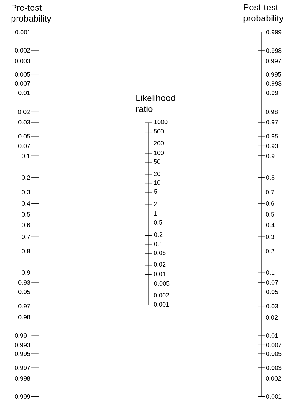
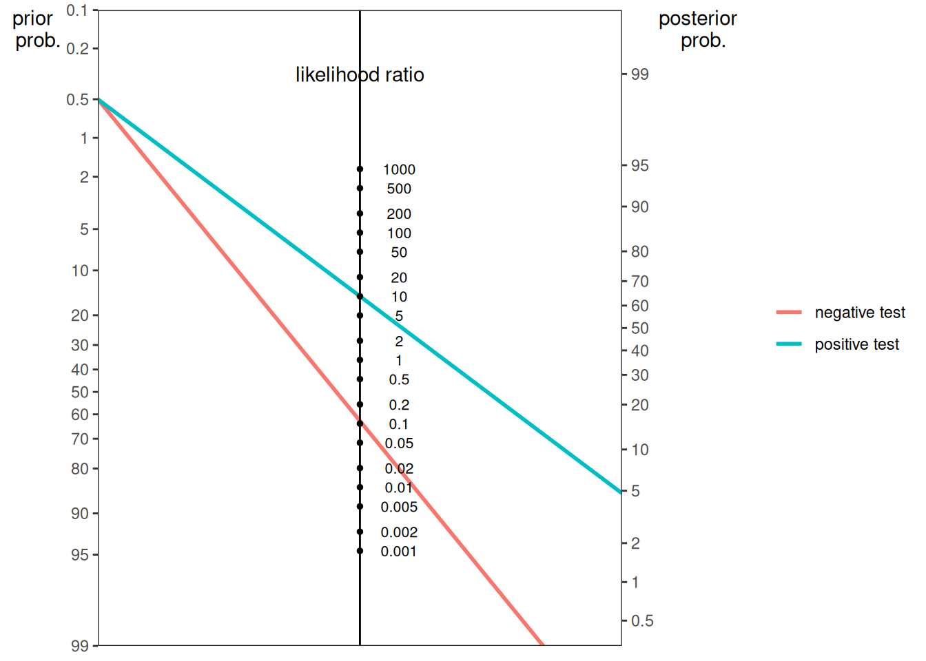
Using Bayes’ theorem (described in Section 16.3.3), solving for posttest odds (based on pretest odds and the likelihood ratio, as in Equation 16.21), and converting odds to probabilities, we can use a Fagan probability nomogram to determine the posttest probability following a test result. The calculation of posttest (posterior) probability is described in Section 17.6.10.29. In its calculation, the probability nomogram automatically converts the pretest probability (i.e., base rate) to prior (pretest) odds and the posterior (posttest) odds to posterior probability, so you do not have to. A probability nomogram (aka Fagan nomogram) is a way of visually applying Bayes’ theorem to determine the posttest probability of having a condition based on the pretest (or prior) probability and likelihood ratio, as depicted in Figure 16.3. To use a probability nomogram, connect the dots from the starting probability (left line) with the likelihood ratio (middle line) to see the updated probability. The updated (posttest) probability is where the connecting line crosses the third, right line.
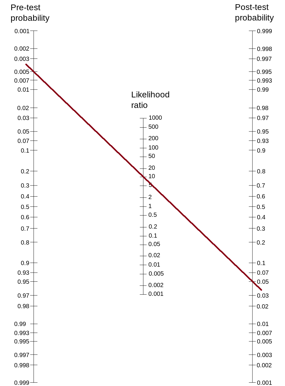
For instance, if the starting probability is 0.5% and the likelihood ratio is 10 (e.g., sensitivity = .90, specificity = .91: \(\text{likelihood ratio} = \frac{\text{sensitivity}}{1 - \text{specificity}} = \frac{.9}{1-.91} = 10\)) from a positive test (i.e., positive likelihood ratio), the updated probability is less than 5%, as depicted in Figure 16.4.
An interactive probability nomogram is available from Altarejos & Hayward (2025) at the following link: https://jamaevidence.mhmedical.com/data/calculators/LR_nomogram.html (archived at https://perma.cc/Z3SW-QMJ3).
The petersenlab package (Petersen, 2025a) contains the petersenlab::posttestProbability() function that estimates the posttest probability of an event, given the pretest probability and the likelihood ratio, or given the pretest probability and the sensitivity (SN) and specificity (SP) of the test.
[1] 0.04784689[1] 0.04784689The function can also estimate the posttest probability of an event given the number of true positives (TP), true negatives (TN), false positives (FP), and false negatives (FN):
We discuss true positives (TP), true negatives (TN), false positives (FP), false negatives (FN), sensitivity (SN), and specificity (SP) in Section 17.6 (Section 17.6.1 and Section 17.6.7).
If the starting probability is 0.5% and the likelihood ratio is 0.11 from a negative test (i.e., negative likelihood ratio), the updated probability is nearly indistinguishable from zero (0.05%).
A probability nomogram calculator is available from Schwartz (2006) at the following link: http://araw.mede.uic.edu/cgi-bin/testcalc.pl (archived at https://perma.cc/X8TF-7YBX). The petersenlab package (Petersen, 2025a) contains the petersenlab::nomogrammer() function that creates a nomogram plot using the positive and negative likelihood ratio or using the sensitivity (SN) and specificity (SP) of the test, as adapted from Chekroud (2017):
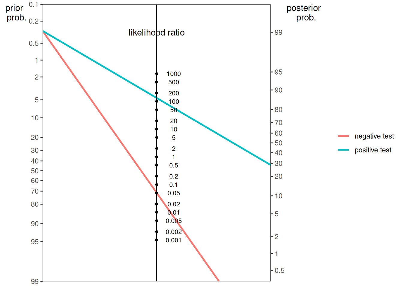
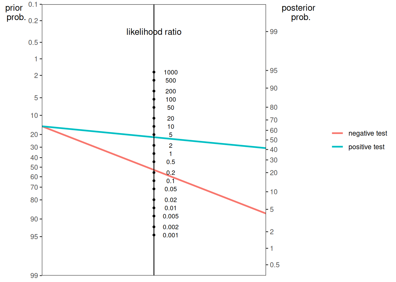
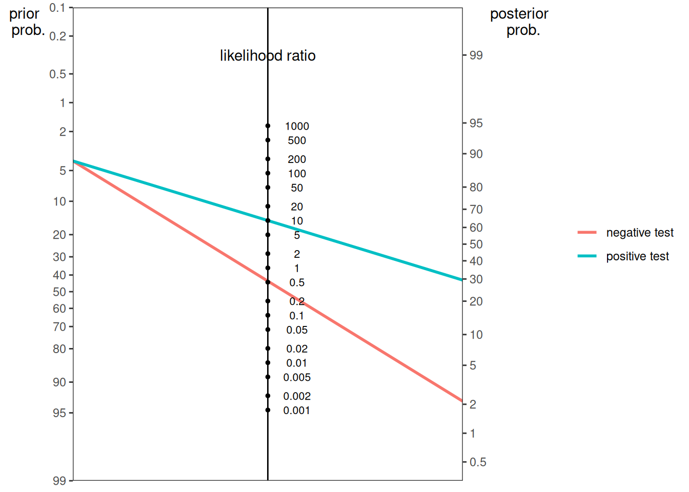
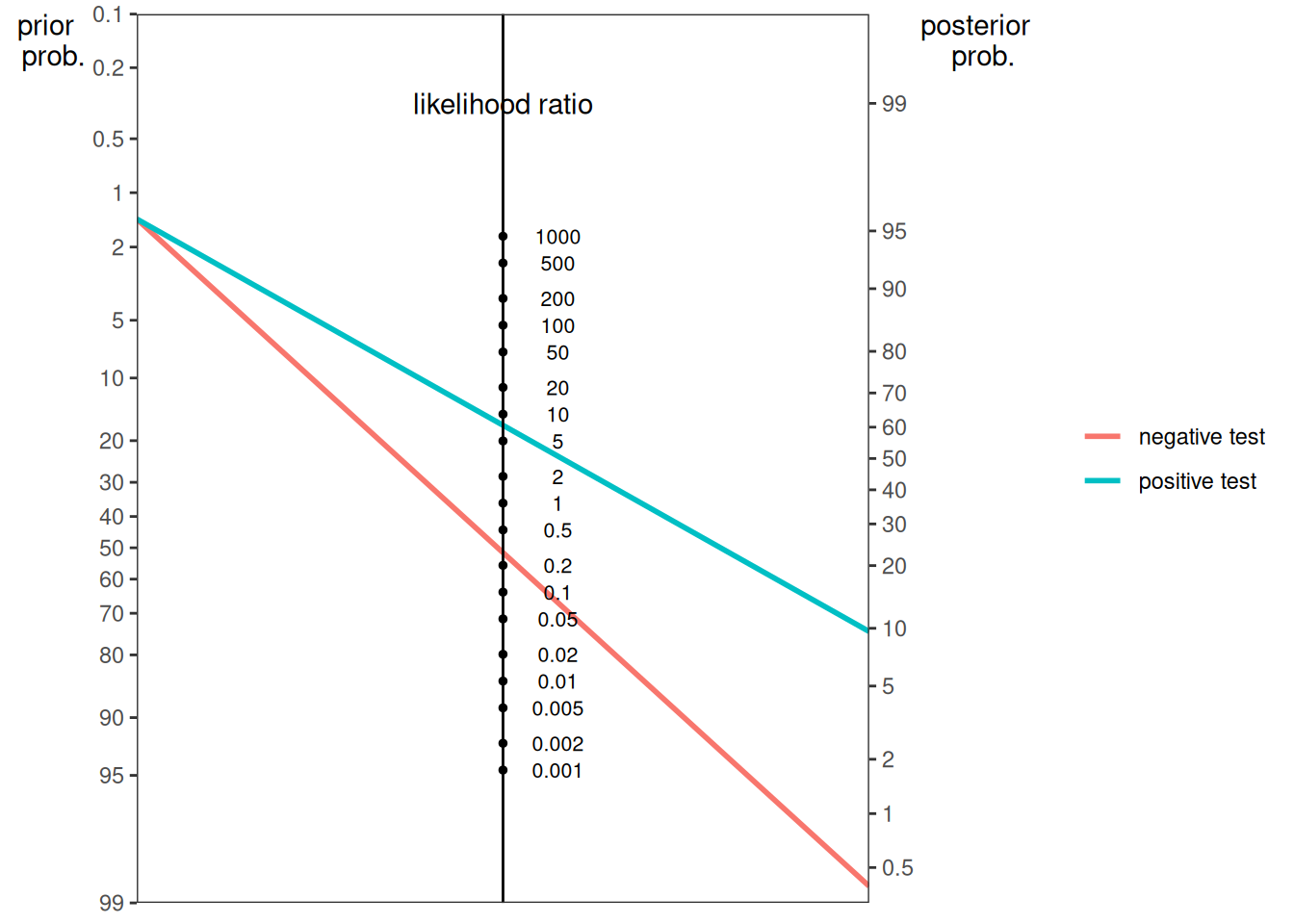
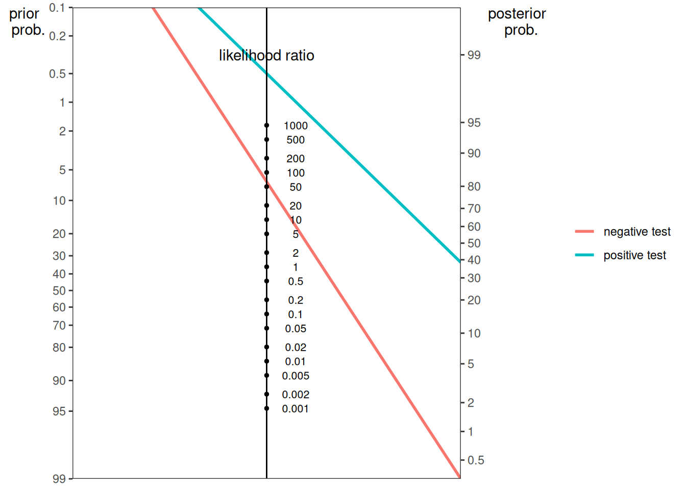
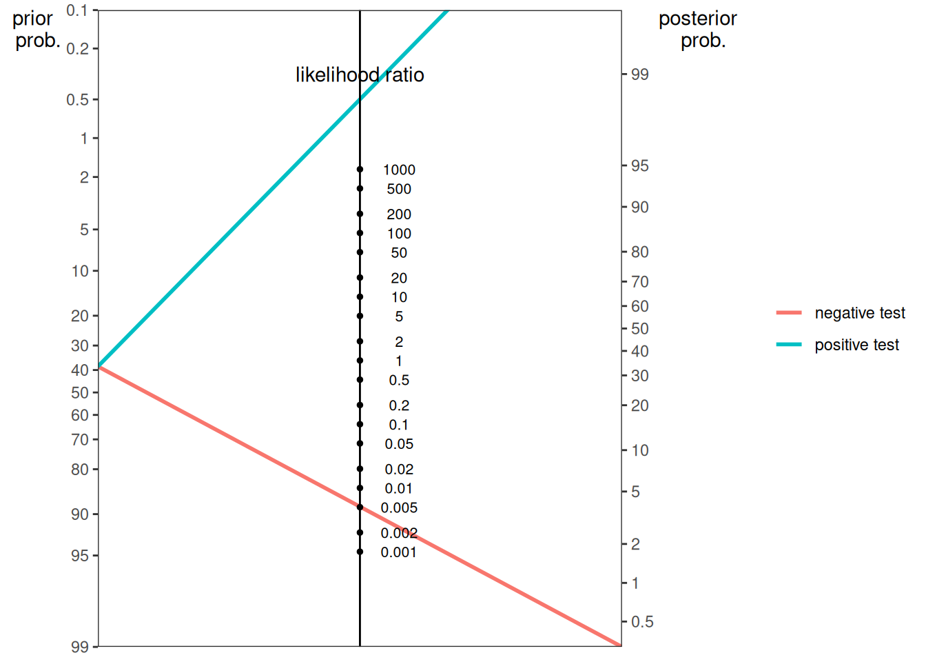
The blue line indicates the posterior probability of the condition given a positive test. The pink line indicates the posterior probability of the condition given a negative test.
The function can also create a nomogram plot using the true positives (TP), true negatives (TN), false positives (FP), and false negatives (FN):
The function can also create a nomogram plot using the sensitivity (SN) and selection rate of the test. Here is a nomogram plot from the HIV example:
Here is a nomogram plot from the cab example (Kahneman, 2011):
The function can also create a nomogram plot using the sensitivity (SN) and false positive rate of the test. Here is a nomogram plot from Example 1 from Silver (2012):
Here is a nomogram plot from Example 2 from Silver (2012):
Here is a nomogram plot from Example 3A from Silver (2012):
Here is a nomogram plot from Example 3B from Silver (2012):
16.8.2.3 Informal Updating
Kahneman (2011) provides the following guidance for an informal approach to updating that anchors predictions to the base rate:
- Start with the “baseline prediction” (i.e., base rate or average outcome).
- Generate or identify your “intuitive prediction”—the number that matches your impression of the evidence.
- Your posterior prediction should fall somewhere between the baseline prediction and the intuitive prediction. “In the default case of no useful evidence, you stay with the baseline [prediction]. At the other extreme, you also stay with your initial [i.e., intuitive] prediction. This will happen, of course, only if you remain completely confident in your initial prediction after a critical review of the evidence that supports it. In most cases you will find some reasons to doubt that the correlation between your intuitive judgment and the truth is perfect, and you will end up somewhere between the two poles.” (pp. 191–192). Base the extent of adjustment (from the baseline prediction) on the magnitude of the correlation between your prediction/evidence and the truth, which acts similar to the likelihood ratio. For instance, if the correlation between your prediction/evidence and the truth is .5, move 50% of the difference from the baseline prediction to the intuitive prediction.
16.9 Conclusion
Fantasy performance—and behavior more generally—is challenging to predict. People commonly demonstrate biases and fallacies when making predictions. People tend to ignore base rates (base rate fallacy) when making predictions. They also tend to confuse inverse conditional probabilities (conditional probability fallacy). Bayes’ theorem provides a way to convert from one conditional probability to its inverse conditional probability using the base rate of each event. There are various ways to account for base rates for more accurate predictions, including through the use of actuarial formulas, Bayesian updating, and more informal approaches. Bayesian updating uses Bayes’ theorem to calculate a posttest probability from a pretest probability and a test result (likelihood ratio). The probability nomogram is a visual approach to Bayesian updating.
16.10 Session Info
R version 4.6.0 (2026-04-24)
Platform: x86_64-pc-linux-gnu
Running under: Ubuntu 24.04.4 LTS

Matrix products: default
BLAS:   /usr/lib/x86_64-linux-gnu/openblas-pthread/libblas.so.3
LAPACK: /usr/lib/x86_64-linux-gnu/openblas-pthread/libopenblasp-r0.3.26.so;  LAPACK version 3.12.0

locale:
 [1] LC_CTYPE=C.UTF-8       LC_NUMERIC=C           LC_TIME=C.UTF-8
 [4] LC_COLLATE=C.UTF-8     LC_MONETARY=C.UTF-8    LC_MESSAGES=C.UTF-8
 [7] LC_PAPER=C.UTF-8       LC_NAME=C              LC_ADDRESS=C
[10] LC_TELEPHONE=C         LC_MEASUREMENT=C.UTF-8 LC_IDENTIFICATION=C

time zone: UTC
tzcode source: system (glibc)

attached base packages:
[1] stats     graphics  grDevices utils     datasets  methods   base

other attached packages:
 [1] lubridate_1.9.5   forcats_1.0.1     stringr_1.6.0     dplyr_1.2.1
 [5] purrr_1.2.2       readr_2.2.0       tidyr_1.3.2       tibble_3.3.1
 [9] ggplot2_4.0.3     tidyverse_2.0.0   psych_2.6.3       petersenlab_1.2.3

loaded via a namespace (and not attached):
 [1] tidyselect_1.2.1    viridisLite_0.4.3   farver_2.1.2
 [4] S7_0.2.2            fastmap_1.2.0       digest_0.6.39
 [7] rpart_4.1.27        timechange_0.4.0    lifecycle_1.0.5
[10] cluster_2.1.8.2     magrittr_2.0.5      compiler_4.6.0
[13] rlang_1.2.0         Hmisc_5.2-5         tools_4.6.0
[16] yaml_2.3.12         data.table_1.18.2.1 knitr_1.51
[19] labeling_0.4.3      htmlwidgets_1.6.4   mnormt_2.1.2
[22] plyr_1.8.9          RColorBrewer_1.1-3  foreign_0.8-91
[25] withr_3.0.2         nnet_7.3-20         grid_4.6.0
[28] stats4_4.6.0        lavaan_0.6-21       xtable_1.8-8
[31] colorspace_2.1-2    scales_1.4.0        MASS_7.3-65
[34] cli_3.6.6           mvtnorm_1.3-7       rmarkdown_2.31
[37] reformulas_0.4.4    generics_0.1.4      otel_0.2.0
[40] rstudioapi_0.18.0   reshape2_1.4.5      tzdb_0.5.0
[43] minqa_1.2.8         DBI_1.3.0           splines_4.6.0
[46] parallel_4.6.0      base64enc_0.1-6     mitools_2.4
[49] vctrs_0.7.3         boot_1.3-32         Matrix_1.7-5
[52] jsonlite_2.0.0      hms_1.1.4           Formula_1.2-5
[55] htmlTable_2.5.0     glue_1.8.1          nloptr_2.2.1
[58] stringi_1.8.7       gtable_0.3.6        quadprog_1.5-8
[61] lme4_2.0-1          pillar_1.11.1       htmltools_0.5.9
[64] R6_2.6.1            Rdpack_2.6.6        mix_1.0-13
[67] evaluate_1.0.5      pbivnorm_0.6.0      lattice_0.22-9
[70] rbibutils_2.4.1     backports_1.5.1     Rcpp_1.1.1-1.1
[73] gridExtra_2.3       nlme_3.1-169        checkmate_2.3.4
[76] xfun_0.57 pkgconfig_2.0.3 