I want your feedback to make the book better for you and other readers. If you find typos, errors, or places where the text may be improved, please let me know. The best ways to provide feedback are by GitHub or hypothes.is annotations.
You can leave a comment at the bottom of the page/chapter, or open an issue or submit a pull request on GitHub: https://github.com/isaactpetersen/Fantasy-Football-Analytics-Textbook
Alternatively, you can leave an annotation using hypothes.is.
To add an annotation, select some text and then click the
symbol on the pop-up menu.
To see the annotations of others, click the
symbol in the upper right-hand corner of the page.
6 Player Evaluation
“It is very difficult to predict—especially the future.”
— Neils Bohr
This chapter provides an overview of some of the many factors in player evaluation. Ultimately, player evaluation involves prediction—predicting how well the player will do in future games.
6.1 Getting Started
6.1.1 Load Packages
6.2 Overview
Evaluating players for fantasy football could be thought of as similar to the process of evaluating companies when picking stocks to buy. You want to evaluate and compare various assets so that you get the assets with the best value.
There are various domains of criteria we can consider when evaluating a football player’s fantasy prospects. Potential domains to consider include:
- athletic profile
- skill
- historical performance
- health
- availability
- age and career stage
- situational factors
- matchups
- cognitive and motivational factors
- fantasy value
The discussion that follows is based on my and others’ impressions of some of the characteristics that may be valuable to consider when evaluating players. However, the extent to which any factor is actually relevant for predicting future performance is an empirical question and should be evaluated empirically.
6.3 Athletic Profile
Factors related to a player’s athletic profile include factors such as:
- body shape
- height
- weight
- hand size
- wing span (arm length)
- body function
- agility
- strength
- speed
- acceleration/explosiveness
- jumping ability
In terms of body shape, we might consider a player’s height, weight, hand size, and wing span (arm length). Height allows players to see over opponents and to reach balls higher in the air. Thus, greater height is particularly valuable for Quarterbacks and Wide Receivers. Heavier players are tougher to budge and to tackle. Greater weight is particularly valuable for Linemen, Fullbacks, and Tight Ends, but it can also be valuable—to a degree—for Quarterbacks, Running Backs, and Wide Receivers. Hand size and wing span is particularly valuable for people catching the ball; thus, a larger hand size and longer wing span are particularly valuable for Wide Receivers and Tight Ends.
In terms of body function, we can consider a player’s agility, strength, speed, acceleration/explosiveness, and jumping ability. For Wide Receivers, speed, explosiveness, and jumping ability are particularly valuable. For Running Backs, agility, strength, speed, and explosiveness are particularly valuable.
Many aspects of a player’s athletic profile, including tests of speed (40-yard dash), strength (bench press), agility (20-yard shuttle run; three cone drill), and jumping ability (vertical jump; broad jump) are available from the National Football League (NFL) Combine, which is especially relevant for evaluating rookies. We demonstrate how to import data from the NFL Combine in Section 4.3.8. There are also calculators that integrate information about body shape and information from the NFL Combine to determine a player’s relative athletic score (RAS) for their position: https://ras.football/ras-calculator/ and https://www.nfl.com/combine/iq/
6.4 Skill
When scouting players, scouts consider not only the player’s athletic profile, but also their position-relevant skill. For instance, how good are they are reading the defense, passing the ball, running routes, catching balls, making defenders miss tackles, taking care of the ball, consistency, etc. Scouting and evaluating skill is a complicated endeavor, and even the professional scouts frequently make mistakes in their evaluations and predictions. You can certainly read skill evaluations about various players; however, unlike metrics of athletic profile, we do not have direct access to the player’s underlying skill. Some may say, “You know it when you see it.” But, this is not particularly useful when trying to identify players who are undervalued or overvalued—because the skill evaluations are likely already “baked into” a player’s projections. Because we do not have direct access to a player’s skill, we tend to rely on indirect metrics of their ability, such as historical performance.
6.5 Historical Performance
6.5.1 Overview
“The best predictor of future behavior is past behavior.” – Unknown
“Past performance does not guarantee future results.” – A common disclaimer about investments.
Factors relating to historical performance to consider could include:
- performance in college
- draft position
- performance in the NFL
- efficiency
- consistency
It is important to consider a player’s past performance. However, the extent to which historical performance may predict future performance may depend on many factors such as (a) the similarity of the prior situation to the current situation, (b) how long ago the prior situation was, and (c) the extent to which the player (or situation) has changed in the interim. For rookies, the player does not have prior seasons of performance in the NFL to draw upon. Thus, when evaluating rookies, it can be helpful to consider their performance in college or in their prior leagues. However, there are large differences between the situation in college and the situation in the NFL, so prior success in college may not portend future success in the NFL. An indicator that intends to be prognostic of future performance, and that accounts for past performance, is a player’s draft position—that is, how early (or late) was a player selected in the NFL Draft. The earlier a player was selected in the NFL Draft, the greater likelihood that the player will perform well; however, this is somewhat countered by the fact that the teams with the highest draft picks tend to be the worst based on the prior season’s record.
For players who have played in the NFL, past performance becomes more relevant because, presumably, the prior situation is more similar (than was their situation in college) to their current situation. Nevertheless, as described below, lots of things change from game to game and season to season, and such changes are important to monitor because they can render prior situations less relevant to the player’s current situation. Thus, it is important not to rely just on a player’s historical performance from last season. Nevertheless, historical performance is one of the best indicators we have.
We demonstrate how to import historical player statistics in Section 4.3.17. We demonstrate how to calculate historical player statistics in Section 4.4.1. We demonstrate how to calculate historical fantasy points in Section 4.4.2.
6.5.1.1 Changes in Situational Factors
Lots of things change from game to game and season to season: injuries, coaches, coaching strategies, teammates, etc. Just because a player performed well or poorly in a given game or season does not necessarily mean that they will perform similarly in subsequent games/seasons. Thus, it is crucial to consider the player’s current situation—and what has changed since the prior game or season. Consider what has changed in terms of situational factors:
- Is the player on a new team?
- Do they have a new head coach or coordinator?
- How will the team’s offensive scheme change?
- Does the team have a better offensive line?
- Does the team have better receiving targets?
- Will the player’s position change on the depth chart?
- Will there be more competition for targets?
- Is there a greater level of competition by opposing teams?
There is often greater uncertainty in selecting a player who has changed teams or whose situation has greatly changed, but such risk can be highly rewarded when the player’s new team or situation is better suited to the player. If a player underachieved on a given team, they may perform better for another team.
6.5.2 Efficiency
In addition to how many fantasy points a player scores in terms of historical performance, we also care about efficiency and consistency. How efficient were they given the number of opportunities they had? This is important to consider because different players have different opportunities. For example, some Running Backs have more opportunity than others (e.g., more carries), so comparing players merely on rushing yards would be misleading. If they were relatively more efficient, they will likely score more points than many of their peers when given more opportunities. If they were relatively inefficient, their capacity to score fantasy points may be more dependent on touches/opportunities. Efficiency might be operationalized by indicators such as yards per passing attempt, yards per rushing attempt, yards per target, yards per reception, yards per route run, etc.
6.5.3 Consistency
In terms of consistency, how consistent was the player from game to game and from season to season? For instance, we could examine the standard deviations of players’ fantasy points across games in a given season. However, the standard deviation tends to be upwardly biased as the mean increases. So, we can account for the player’s mean fantasy points per game by dividing their game-to-game standard deviation of fantasy points (\(s_x\) or \(\sigma_x\)) by their mean fantasy points across games (\(\bar{x}\) or \(\mu_x\)). This is known as the coefficient of variation (CV), which is provided in Equation 6.1.
\[ \text{CV} = \frac{s_x}{\bar{x}} \tag{6.1}\]
Players with a lower standard deviation and a lower coefficient of variation (of fantasy points across games) are more consistent. In the example below, Player 2 might be preferable to Player 1 because Player 2 is more consistent; Player 1 is more “boom-or-bust.” Despite showing a similar mean of fantasy points across weeks, Player 2 shows a smaller week-to-week standard deviation and coefficient of variation.
Code
set.seed(1)

playerScoresByWeek <- data.frame(
  player1_scores = rnorm(17, mean = 20, sd = 7),
  player2_scores = rnorm(17, mean = 20, sd = 4),
  player3_scores = rnorm(17, mean = 10, sd = 4),
  player4_scores = rnorm(17, mean = 10, sd = 1)
)

consistencyData <- data.frame(t(playerScoresByWeek))

weekNames <- paste("week", 1:17, sep = "")

names(consistencyData) <- weekNames
row.names(consistencyData) <- NULL

consistencyData$mean <- rowMeans(consistencyData[,weekNames])
consistencyData$sd <- apply(consistencyData, 1, sd)
consistencyData$cv <- consistencyData$sd / consistencyData$mean

consistencyData$player <- c(1, 2, 3, 4)

consistencyData <- consistencyData %>%
  select(player, mean, sd, cv, week1:week17)

round(consistencyData, 2)
However, another perspective is to embrace the chaos and uncertainty that is part of fantasy football; one is better positioned to win a given week if you have one or a few players that “go off”—i.e., that score lots of points. Thus, starting boom-or-bust players can make it more likely that you win in the “boom weeks”; however, this may also mean having some “bust weeks”.
6.6 Health
Health-related factors to consider include:
- current injury status
- injury history
It is also important to consider a player’s past and current health status. In terms of a player’s current health status, it is important to consider whether they are injured or are playing at less than 100% of their typical health. In terms of a player’s prior health status, one can consider their injury history, including the frequency and severity of injuries and their prognosis.
We demonstrate how to import injury reports in Section 4.3.18.
6.7 Availability
In addition to injuries, other factors can affect a player’s availability, including contract hold-outs or league suspensions, for instance, due to violating the league’s conduct policy. Some players may be “holding out”, which means that they may refuse to play until they sign a more desirable contract with the team (e.g., for more money or for a longer-term contract).
6.8 Age and Career Stage
Age and career stage-related factors include:
- age
- experience
- touches
A player’s age is relevant because of important age-related changes in a player’s speed, ability to recover from injury, etc. A player’s experience is relevant because players develop knowledge and skills with greater experience. A player’s prior touches/usage is also relevant, because it speaks to how many hits a player may have taken. For players who take more hits, it may be more likely that their bodies “break down” sooner.
6.9 Situational Factors
Situational factors one could consider include:
- team quality
- quality of the team’s offense
- quality of the team’s defense
- role on team
- teammates
- opportunity and usage
- snap count
- touches/targets
- red zone usage
Football is a team sport. A player is embedded within a broader team context; it is important to consider the strength of their team context insofar as it may support— or detract from—a player’s performance. For instance, for a Quarterback, it is important to consider how strong the pass blocking is from the Offensive Line. Will they have enough time to throw the ball, or will they be constantly under pressure to be sacked? It is also important to consider the strength of the pass catchers—the Wide Receivers and Tight Ends. For a Running Back, it is important to consider how strong the run blocking is from the Offensive Line. For a Wide Receiver, it is important to consider how strong the pass blocking is, and how strong the Quarterback is. In general, offensive players benefit from being on stronger offenses, so it can make sense to draft players (onto your fantasy team) that are on strong offenses. In addition, offensive players can also benefit from being on teams with weaker defenses because that may force the offense to score more points.
It is also important to consider a player’s role on the team. Is the player a starter or a backup? Related to this, it is important to consider the strength of one’s teammates. For a given Running Back, if a teammate is better at running the ball, this may take away from how much the player sees the field. For a given Wide Receiver, if a teammate is better at catching the ball, this may take some targets away from the player. However, the team’s top defensive back is often matched up against the team’s top Wide Receiver. So, if the team’s top Wide Receiver is matched up against a particularly strong Defensive Back, the second- and third-best Wide Receivers may more targets than usual.
It is also important to consider a player’s opportunity, usage, and volume, which are influenced by many factors, including the skill of the player, the skill of their teammates, the role of the player on the team, the coaching style, the strategy of the opposing team, game scripts, etc. In terms of the player’s opportunity and usage, how many snaps do they get? How many routes do they run? How many touches and/or targets do they receive? Being on the field for more snaps, running more routes, and receiving more touches and/or targets means that the player has more opportunities to score fantasy points. What is the depth of their targets? Are they receiving short passes or long passes? Players who receive longer passes may have an opportunity for more fantasy points but also may be more volatile (i.e., less consistent). Are they targeted in the red zone? Red zone targets are more likely to lead to touchdown scoring opportunities, which are particularly valuable in fantasy football.
6.10 Matchups
Matchup-related factors to consider include:
- strength of schedule
- weekly matchup
Another aspect to consider is how challenging their matchup(s) and strength of schedule is. For a Quarterback, it is valuable to consider how strong the opponent’s passing defense is. For a Running Back, how strong is the running defense? For a Wide Receiver, how strong is the passing defense and the Defensive Back that is likely to be assigned to guard them?
6.11 Cognitive and Motivational Factors
Other factors to consider include cognitive and motivational factors. Some coaches refer to these as the “X Factor” or “the intangibles.” However, just as any other construct in psychology, we can devise ways to operationalize them. Insofar as they are observable, they are measurable.
Cognitive and motivational factors one could consider include:
- reaction time
- knowledge and intelligence
- work ethic and mental toughness
- competitiveness and “will to win”
- incentives
- contract performance incentives
- whether they are in a contract year
A player’s knowledge, intelligence, and reaction time can help them gain an upper-hand even when they may not be the fastest or strongest. The Wonderlic test was formerly used to assess a player’s cognitive abilities (O’Connell, 2022; archived at https://web.archive.org/web/20220303015018/https://www.nytimes.com/2022/03/02/sports/football/nfl-wonderlic-test.html). A player’s work ethic and mental toughness may help them be resilient and persevere in the face of challenges. The extent to which the player has a competitiveness, drive, or “will to win” may also influence their performance. Contact-related incentives may lead a player to put forth greater effort. For instance, a contract may have a performance incentive that provides a player greater compensation if they achieve a particular performance milestone (e.g., receiving yards). Another potential incentive is if a player is in what is called their “contract year” (i.e., the last year of their current contract). If a player is in the last year of their current contract, they have an incentive to perform well so they can get re-signed to a new contract. We discuss the potential influences of being in a contract year in Chapter 18.
6.12 Fantasy Value
6.12.1 Sources From Which to Evaluate Fantasy Value
There are several sources that one can draw upon to evaluate a player’s fantasy value:
- expert or aggregated rankings
-
layperson rankings
- players’ Average Draft Position (ADP) in other league snake drafts
- players’ Average Auction Value (AAV) in other league auction drafts
- expert or aggregated projections
6.12.1.1 Expert Fantasy Rankings
Fantasy rankings (by so-called “experts”) are provided by many sources. To reduce some of the bias due to a given source, some services aggregate projections across sources, consistent with a “wisdom of the crowd” approach. FantasyPros aggregates fantasy rankings across sources. Fantasy Football Analytics creates fantasy rankings from projections that are aggregated across sources (see the webapp here: https://apps.fantasyfootballanalytics.net). There are also sites that aggregate rankings from both fantasy football analysts and from sportsbooks, which are based on Vegas lines and how people bet: https://www.evsharps.com/ranks?format=std.
6.12.1.2 Layperson Fantasy Rankings: ADP and AAV
Average Draft Position (ADP) and Average Auction Value (AAV), are based on league drafts, mostly composed of everyday people. ADP is based on snake drafts, whereas AAV is based on auction drafts. Thus, ADP and AAV are consistent with a “wisdom of the crowd” approach, and I refer to them as forms of rankings by laypeople. ADP data are provided by FantasyPros. AAV data are also provided by FantasyPros.
6.12.1.3 Projections
Projections are provided by various sources. Projections (and rankings, for that matter) are a bit of a black box. It is often unclear how they were derived by a particular source. That is, it is unclear how much of the projection was based on statistical analysis versus conjecture.
To reduce some of the bias due to a given source, some services aggregate projections across sources, consistent with a “wisdom of the crowd” approach. Projections that are aggregated across sources are provided by Fantasy Football Analytics (see the webapp here: https://apps.fantasyfootballanalytics.net) and by FantasyPros. There are also sites that aggregate projections from both fantasy football analysts and from sportsbooks, which are based on Vegas lines and how people bet: https://www.evsharps.com/ranks?format=std. Moreover, sites also provide season-long player futures for the over/under betting lines: https://www.rotowire.com/betting/nfl/player-futures.php; https://www.evsharps.com/futures. In addition, sites also provide weekly projections based on Vegas lines: https://vegasprojections.com; https://www.actionnetwork.com/nfl/props; https://tools.32beatwriters.com; https://the-odds-api.com.
We demonstrate how to download fantasy football projections in Section 4.3.27.
6.12.1.4 Benefits of Using Projections Rather than Rankings
It is important to keep in mind that rankings, ADP, and AAV are specific to roster and scoring settings of a particular league. For instance, in point-per-reception (PPR) leagues, players who catch lots of passes (Wide Receivers, Tight Ends, and some Running Backs) are valued more highly. As another example, Quarterbacks are valued more highly in 2-Quarterback leagues. Thus, if using rankings, ADP, or AAV, it is important to find ones from leagues that mirror—as closely as possible—your league settings.
Projected statistics (e.g., projected passing touchdowns) are agnostic to league settings and can thus be used to generate league-specific fantasy projections and rankings. Thus, projected statistics may be more useful than rankings because they can be used to generate rankings for your particular league settings. For instance, if you know how many touchdowns, yards, and interceptions a Quarterback is a projected to throw (in addition to any other relevant categories for the player, e.g., rushing yards and touchdowns), you can calculate how many fantasy points the Quarterback is expected to gain in your league (or in any league). Thus, you can calculate ranking from projections, but you cannot reverse engineer projections from rankings. Moreover, projections have been shown to be more accurate than rankings (Petersen, 2016; archived at https://perma.cc/KEZ9-WRB6). When you have projections, you can perform valuable simulations of players’ expected performance, as exemplified in Chapter 24.
6.12.2 Indices to Evaluate Fantasy Value
Based on the sources above (rankings, ADP, AAV, and projections), we can derive multiple indices to evaluate fantasy value. There are many potential indices that can be worthwhile to consider, including a player’s:
6.12.2.1 Dropoff
A player’s dropoff is the difference between (a) the player’s projected points and (b) the projected points of the next-best player at that position.
6.12.2.2 Value Over Replacement Player
Because players from some positions (e.g., Quarterbacks) tend to score more points than players from other positions (e.g., Wide Receivers), it would be inadvisable to compare players across different positions based on projected points. In order to more fairly compare players across positions, we can consider a player’s value over a typical replacement player at that position (shortened to “value over replacement player”). A player’s value over a replacement player (VORP) is the difference between (a) a player’s projected fantasy points and (b) the fantasy points that you would be expected to get from a typical bench player at that position. Thus, VORP provides an index of how much added value a player provides.
6.12.2.3 Uncertainty
A player’s uncertainty is how much variability there is in projections or rankings for a given player across sources. For instance, consider a scenario where three experts provide ratings about two players, Player A and Player B. Player A is projected to score 300, 310, and 290 points by experts 1, 2, and 3, respectively. Player B is projected to score 400, 300, and 200 points by experts 1, 2, and 3, respectively. In this case, both players are (on average) projected to score the same number of points (300).
Code
exampleData <- data.frame(
  player = c(rep("A", 3), rep("B", 3)),
  expert = c(1:3, 1:3),
  projectedPoints = c(300, 310, 290, 400, 300, 200)
)

playerA_mean <- mean(exampleData$projectedPoints[which(exampleData$player == "A")])
playerB_mean <- mean(exampleData$projectedPoints[which(exampleData$player == "B")])

playerA_sd <- sd(exampleData$projectedPoints[which(exampleData$player == "A")])
playerB_sd <- sd(exampleData$projectedPoints[which(exampleData$player == "B")])

playerA_cv <- playerA_mean / playerA_sd
playerB_cv <- playerB_mean / playerB_sdHowever, the players differ considerably in their uncertainty (i.e., the source-to-source variability in their projections), as operationalized with the standard deviation and coefficient of variation of projected points across sources for a given player.
Here is a depiction of a density plot of projected points for a player with a low, medium, and high uncertainty:
Code
playerA <- rnorm(1000000, mean = 150, sd = 5)
playerB <- rnorm(1000000, mean = 150, sd = 15)
playerC <- rnorm(1000000, mean = 150, sd = 30)

mydata <- data.frame(playerA, playerB, playerC)

mydata_long <- mydata %>%
  pivot_longer(
    cols = everything(),
    names_to = "player",
    values_to = "points"
  ) %>%
  mutate(
    name = case_match(
      player,
      "playerA" ~ "Player A",
      "playerB" ~ "Player B",
      "playerC" ~ "Player C",
    )
  )

ggplot2::ggplot(
  data = mydata_long,
  ggplot2::aes(
    x = points,
    fill = name
  )
) +
  ggplot2::geom_density(alpha = .3) +
  ggplot2::labs(
    x = "Players' Projected Points",
    title = "Density Plot of Projected Points for Three Players"
  ) +
  ggplot2::theme_classic() +
  ggplot2::theme(legend.title = element_blank())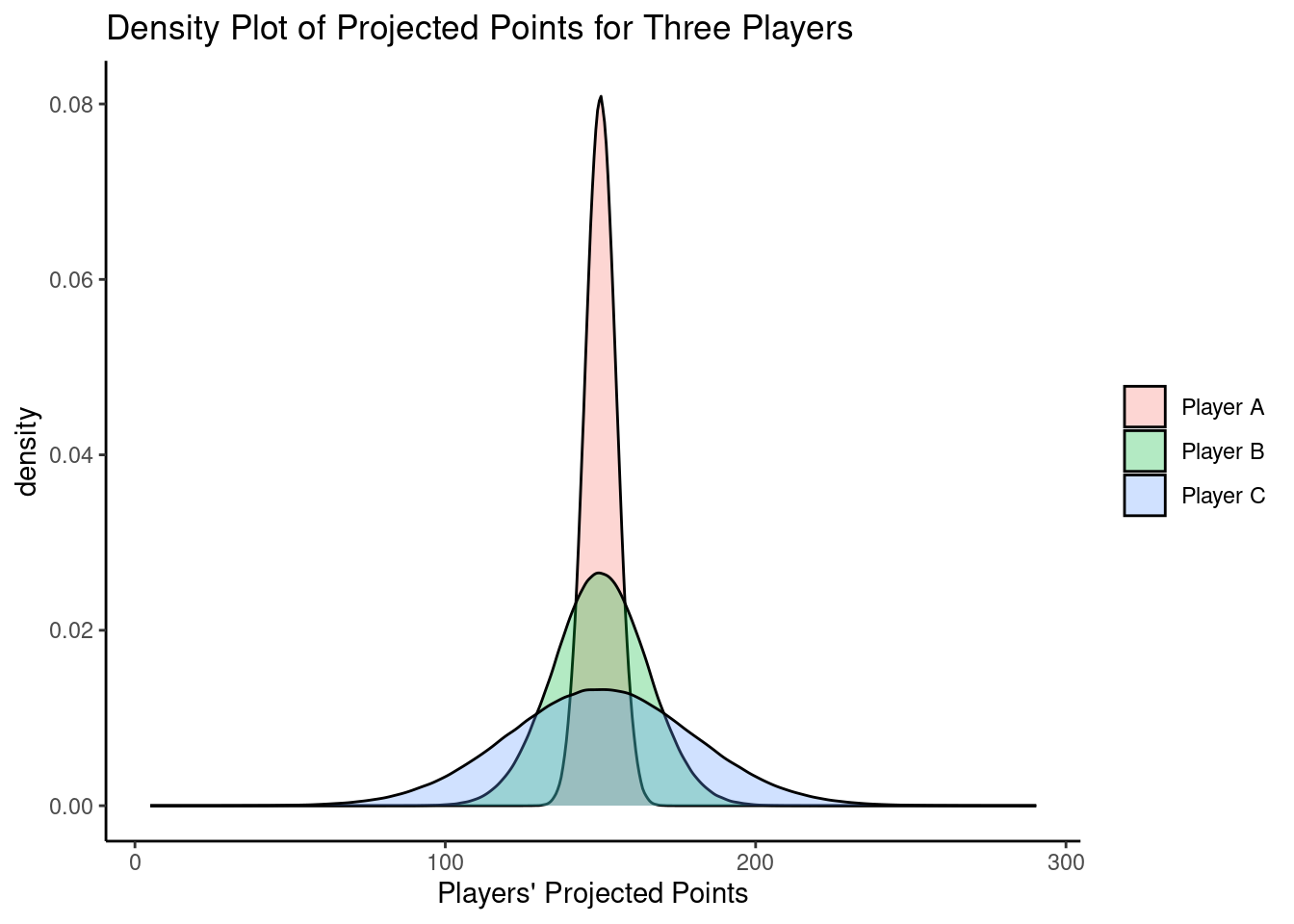
Uncertainty is not necessarily a bad characteristic of a player’s projected points. It just means we have less confidence about how the player may be expected to perform. Thus, players with greater uncertainty are risky and tend to have a higher upside (or ceiling) and a lower downside (or floor). For this reason, identifying players with a high uncertainty can be useful for identifying potential “sleepers”—i.e., late-round draft picks who outperform expectations (Petersen, 2014; archived at https://perma.cc/K6LX-85A4).
6.13 Signs Versus Samples
When thinking about the most important domains to assess for evaluating players and predicting their performance, it is important to distinguish between signs and samples (Den Hartigh et al., 2018). Signs are indicators of underlying states. The signs approach to assessment involves assessing processes that may predict performance, where the emphasis is on what the sign indicates about the underlying attribute, rather than on the specific behavior itself. In football, the signs approach might involve measuring skills using separate tests where players’ skills are tested separately (i.e., in isolation from other skills) in controlled settings. For instance, the NFL Combine takes a signs approach to assessment, in which players have a separate test to assess for speed (e.g., 40-yard dash) and jumping ability (e.g., vertical jump). The signs approach to assessment assumes that the various skills assessed (e.g., being fast, being able to jump high, having strong endurance, being motivated) have high predictive validity for the target behavior (i.e., future performance in games; Den Hartigh et al., 2018).
Samples reflect behaviors that are close to the behavior of interest. The samples approach to asesssment tries to assess the person’s performance in a behavior, situation, and context that are as reflective as possible of the kinds of behaviors, situations, and contexts that the person would have to perform in for the position or occupation. In the samples approach, the behavior itself is the main emphasis, rather than an underlying attribute. In football, the samples approach might involve measuring the player’s performance during games or game-like situations. For instance, to assess the skills of a Wide Receiver, you might observe—during games or game-like situations—how well they are able to catch passes when closely guarded or double-teamed, or how well they are able to catch poorly thrown passes.
In general, samples tend to be stronger than signs for predicting player performance in sports (Den Hartigh et al., 2018). For instance, compared to tests of speed, power, and agility at the NFL Combine, collegiate performance is a stronger predictor of performance in the NFL (Lyons et al., 2011). That is, previous sports performance is the best predictor of future performance (for a review, see Den Hartigh et al., 2018).
According to the theoretical perspective to sports performance known as the ecological dynamics approach, successful performance in sports involves the coordination of multiple, intertwined skills that are contextually embedded (Den Hartigh et al., 2018). For instance, a Wide Receiver needs to coordinate skills in speed, route running, jumping, and good hands to create space from defenders and to catch poorly thrown passes in a game. The ecological dynamics approach considers the important interaction of the player, task, and environment. Thus, to assess players in a way that is likely to be most predictive of their future performance, it is important for the assessment to retain the player–task–environment interaction (Den Hartigh et al., 2018). For example, it would be valuable to use assessments from games or game-like situations in which players must perform tasks that leverage multiple, intertwined skills and that are similar to the tasks you want to predict. The extent to which the assessments are more reflective of games or game-like situations, we consider the assessment to have better ecological validity.
6.14 Putting it Altogether
After performing an evaluation of the relevant domain(s) for a given player, one must integrate the evaluation information across domains to make a judgment about a player’s overall value. When considering how much weight to give to each of various factors, it is important to evaluate how much predictive validity each factor has for predicting a player’s successful performance in the NFL. Then, one can weight each variable according to its predictive validity using an actuarial approach. Actuarial approaches are described in a later chapter, in Section 15.2.2. For now, suffice it to say that actuarial approaches leverage statistical formulas, as opposed to using judgment alone. As described in Chapter 14, people’s judgment—including judgments by experts (e.g., professional scouts and coaches)—tends to be riddled with biases (Den Hartigh et al., 2018). Moreover, experts tend to disagree in terms of their judgments/predictions about players (Den Hartigh et al., 2018). In addition, there are benefits to leveraging multiple perpectives, consistent with the “wisdom of the crowd”, as described in Section 26.3. In general, as noted in Section 6.13, give more weight to samples of relevant behavior—such as past performance in games—than to signs such as NFL Combine metrics (e.g., bench press, 40-yard dash, etc.). Where you can, use assessments from games or game-like situations in which players must perform tasks that leverage multiple, intertwined skills and that are similar to the tasks you want to predict.
When thinking about a player’s value, it can be worth thinking of a player’s upside and a player’s downside. Players that are more consistent may show higher downside but a lower upside. Younger, less experienced players may show a higher upside but a lower downside.
The extent to which you prioritize a higher upside versus a higher downside may depend on many factors. For instance, when drafting players, you may prioritize drafting players with the highest downside (i.e., the safest players), whereas you may draft sleepers (i.e., players with higher upside) for your bench. When choosing which players to start in a given week, if you are predicted to beat a team handily, it may make sense to start the players with the highest downside. By contrast, if you are predicted to lose to a team by a good margin, it may make sense to start the players with the highest upside.
6.15 Conclusion
In conclusion, there are many factors to consider when evaluating players. You will have less direct access to some factors (e.g., cognitive and motivational factors) than others (e.g., historical performance). When considering how much weight to give to each of various factors, it is important to evaluate how much predictive validity each factor has for predicting a player’s successful performance, and to weight it accordingly. In general, samples tend to be stronger than signs for predicting player performance in sports. For instance, compared to tests of speed, power, and agility at the NFL Combine, collegiate performance is a stronger predictor of performance in the NFL. That is, previous sports performance is the best predictor of future performance. When thinking about a player’s value, it can be worth thinking their potential upside and downside. Whether you value a player with higher upside or higher downside may depend on many factors such as, when drafting, whether you are seeking a starter or bench player, and, when in-season, whether you are projected to win by a large margin in your matchpup.
6.16 Session Info
R version 4.6.1 (2026-06-24)
Platform: x86_64-pc-linux-gnu
Running under: Ubuntu 24.04.4 LTS

Matrix products: default
BLAS:   /usr/lib/x86_64-linux-gnu/openblas-pthread/libblas.so.3
LAPACK: /usr/lib/x86_64-linux-gnu/openblas-pthread/libopenblasp-r0.3.26.so;  LAPACK version 3.12.0

locale:
 [1] LC_CTYPE=C.UTF-8       LC_NUMERIC=C           LC_TIME=C.UTF-8
 [4] LC_COLLATE=C.UTF-8     LC_MONETARY=C.UTF-8    LC_MESSAGES=C.UTF-8
 [7] LC_PAPER=C.UTF-8       LC_NAME=C              LC_ADDRESS=C
[10] LC_TELEPHONE=C         LC_MEASUREMENT=C.UTF-8 LC_IDENTIFICATION=C

time zone: UTC
tzcode source: system (glibc)

attached base packages:
[1] stats     graphics  grDevices utils     datasets  methods   base

other attached packages:
 [1] lubridate_1.9.5 forcats_1.0.1   stringr_1.6.0   dplyr_1.2.1
 [5] purrr_1.2.2     readr_2.2.0     tidyr_1.3.2     tibble_3.3.1
 [9] ggplot2_4.0.3   tidyverse_2.0.0

loaded via a namespace (and not attached):
 [1] gtable_0.3.6       jsonlite_2.0.0     compiler_4.6.1     tidyselect_1.2.1
 [5] scales_1.4.0       yaml_2.3.12        fastmap_1.2.0      R6_2.6.1
 [9] labeling_0.4.3     generics_0.1.4     knitr_1.51         htmlwidgets_1.6.4
[13] pillar_1.11.1      RColorBrewer_1.1-3 tzdb_0.5.0         rlang_1.3.0
[17] stringi_1.8.7      xfun_0.60          S7_0.2.2           otel_0.2.0
[21] timechange_0.4.0   cli_3.6.6          withr_3.0.3        magrittr_2.0.5
[25] digest_0.6.39      grid_4.6.1         hms_1.1.4          lifecycle_1.0.5
[29] vctrs_0.7.3        evaluate_1.0.5     glue_1.8.1         farver_2.1.2
[33] rmarkdown_2.31     tools_4.6.1        pkgconfig_2.0.3    htmltools_0.5.9