I want your feedback to make the book better for you and other readers. If you find typos, errors, or places where the text may be improved, please let me know. The best ways to provide feedback are by GitHub or hypothes.is annotations.
You can leave a comment at the bottom of the page/chapter, or open an issue or submit a pull request on GitHub: https://github.com/isaactpetersen/Fantasy-Football-Analytics-Textbook
Alternatively, you can leave an annotation using hypothes.is.
To add an annotation, select some text and then click the
symbol on the pop-up menu.
To see the annotations of others, click the
symbol in the upper right-hand corner of the page.
20 Modern Portfolio Theory
This chapter provides an overview of modern portfolio theory.
20.1 Getting Started
20.1.1 Load Packages
20.1.2 Load Data
Code
load(file = "./data/players_projectedPoints_seasonal.RData")
load(file = "./data/player_stats_seasonal.RData")
load(file = "./data/player_stats_weekly.RData")
load(file = "./data/nfl_actualFantasyPoints_weekly.RData")
load(file = "./data/nfl_playerIDs.RData")
load(file = "./data/nfl_schedules.RData")
We created the player_stats_weekly.RData and player_stats_seasonal.RData objects in Section 4.4.3.
20.2 Overview
20.3 Fantasy Football is Like Stock Picking
Selecting players for your fantasy team is like picking stocks. In both fantasy football and the stock market, your goal is to pick assets (i.e., players/stocks) that will perform best and that others undervalue. But what is the best way to do that? Below, we discuss approaches to picking players/stocks.
20.3.1 The Wisdom of the Crowd (or Market)
In picking players, there are various approaches one could take. You could do lots of research to pick players/stocks with strong fundamentals that you think will do particularly well next year. By picking these players/stocks, you are predicting that they will outperform their expectations. However, all of your information is likely already reflected in the current valuation of the player/stock, so your prediction is basically a gamble. This is evidenced by the fact that people do not reliably beat the crowd/market.
Even so-called experts do not beat the market reliably. There is little consistency in the performance of mutual fund managers over time. In the book, “The Drunkard’s Walk: How Randomness Rules Our Lives”, Mlodinow (2008) reported essentially no correlation between performance of the top mutual funds in a five-year period with their performance over the subsequent five years. That is, the best funds in a one period were not necessarily the best funds in another period. This suggests that mutual fund managers differ in great part because of luck or chance rather than reliable skill. In any given year, some mutual funds will do better than other mutual funds. But this overperformance in a given year likely reflects more randomness than skill. That is likely why a cat beat professional investors in a stock market challenge (Goldstein, 2013; archived at https://perma.cc/R3XU-K6J8). That is, “few stock pickers, if any, have the skill needed to beat the market consistently, year after year” (Kahneman, 2011, p. 214). Although our sample size is much smaller with fantasy football projections, there also appears to be little consistency in fantasy football sites’ rank in accuracy over time (Kartes, 2024; archived at https://perma.cc/69F7-LLTN; Petersen, 2017; archived at https://perma.cc/BG2W-ANUF), suggesting that the projection sources are not reliably better than each other (or the crowd) over time.
The market reflects all of the knowledge of the crowd. One common misconception is that if you go with the market, you will receive “average” returns (by “average”, I mean that you will be in the 50th percentile among investors). This is not true—it has been shown that most mutual funds (about 80%) underperform the average returns of the stock market. So, by going with the market average, you will likely perform better than the “average” fund/investor. Consistent with this, crowd-averaged fantasy football projections tend to be more accurate than any individual’s projection (Kartes, 2024; archived at https://perma.cc/69F7-LLTN; Petersen, 2017; archived at https://perma.cc/BG2W-ANUF). This evidence is consistent with the notion of the wisdom of the crowd, described in Section 26.3. Moreover, even if the stock market is relatively accurate (“efficient”) in terms of valuing stocks based on all (publicly) available information (i.e., the efficient market hypothesis), your fantasy football league is likely not. Thus, it may be effective to use crowd-based projections to identify players who are undervalued by your league.
20.3.2 Diversification
Modern portfolio theory (mean-variance theory) is a framework for determining the optimal composition of an investment portfolio to maximize expected returns for a given level of risk. Here, risk refers to the variability (e.g., standard deviation or variance) of returns across time. Given two portfolios with the same expected returns over time, people tend to prefer the “safer” portfolio—that is, the portfolio with less variability/volatility across time. One of the powerful notions of modern portfolio theory is that, through diversification, one can achieve lower risk with the same expected returns. In investing, diversification involves owning multiple asset classes (e.g., domestic and international stocks and bonds), with the goal of having asset classes that are either uncorrelated or negatively correlated. That is, owning different types of assets is safer than owning only one type. If you have too much money in one asset and that asset tanks, you will lose your money. In other words, you do not want to put all of your eggs in one basket. By owning different asset classes, you can limit your downside risk without sacrificing much in terms of expected return. In sum, the goal of diversification is to reduce risk (not to increase returns) and thus to increase risk-adjusted returns, by reducing the amount of risk needed for a given level of return.
This lesson can also apply to fantasy football. When assembling a team, you are essentially putting together a portfolio of assets (i.e., team of players). As with stocks, each player has an expected return (i.e., projection) and a degree of risk. In fantasy football, a player’s risk might be quantified in terms of the variability of projected scores for a player across projection sources (e.g., Projection Source A, Source B, Source C, etc.), or as historical game-to-game variability. Variability of projected scores for a player across projection sources could reflect the uncertainty of projections for a player. Variability of historical (actual) fantasy points across games could reflect many factors, including risks due to injuries, situational changes (e.g., being traded to a new team or changes in team composition such as due to the acquisition of new players on the team), game scripts, and the tendency for the player to be “boom-or-bust” (e.g., if they are highly dependent on scoring touchdowns or long receptions for fantasy points). All things equal, we want to minimize our risk for a given level of expected returns. That way, we have the best chance of winning any given week. For the same level of expected returns, higher risk teams might have a few amazing games, but their teams might fall flat in other weeks. That is, for a given (high) rate of return, you are best off in the long run (i.e., over the course of a season) with a lower risk team compared to a higher risk team (Hitchings, 2012; archived at https://perma.cc/NE35-G6LR).
In terms of diversification, it can be helpful to diversify in multiple ways. First, it can be helpful not to rely on just one or two “stud” players. If they are on bye or have a down week, your team is more likely to suffer. Another way to diversify is to draft players with different bye weeks so you do not have multiple starting players on bye in a given week. Also, there are risks in picking multiple offensive players from the same team. If you draft your starting Quarterback and Wide Receiver from the same team (e.g., the Cowboys), you are exposing your fantasy team to considerable risk. For instance, if you have the Quarterback and Wide Receiver from the same team, and the team has a poor offensive outing, that will have a greater impact. You can limit your downside risk by diversifying—drafting players from different teams. That way if the Cowboys’ offense does poorly in a given week, your fantasy team will not be as affected. Having multiple players on a juggernaut offense can be a boon, but it can be challenging to predict which offense will lead the league.
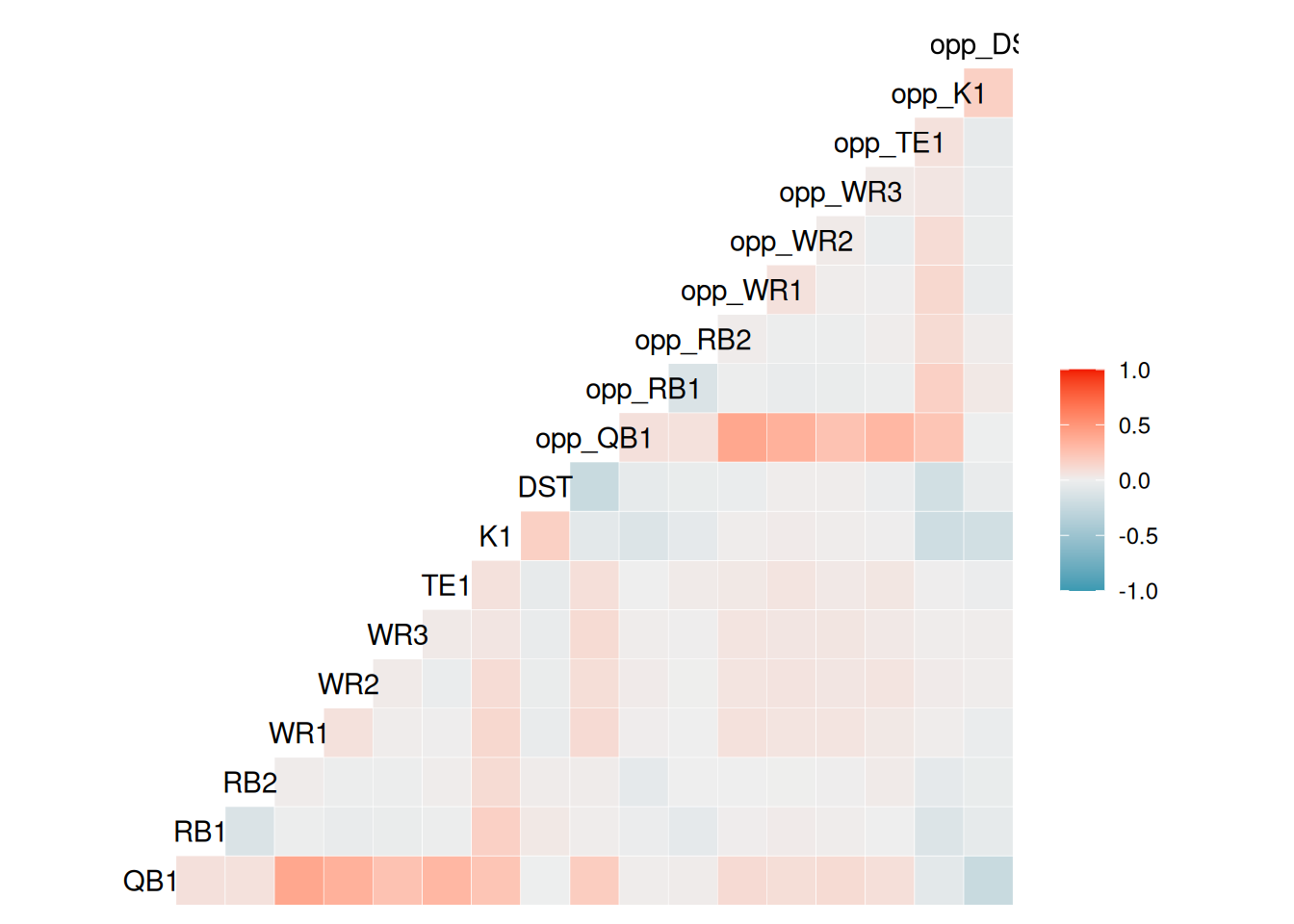
However, sometimes having two players on the same team might be beneficial because some positions may be uncorrelated or even negatively correlated, which can also reduce risk. For instance, the performance of the Tight End and Running Back on the same team tends to be slightly negatively correlated, so it might not be a bad idea to start the Tight End and Running Back from the same team. For a correlation matrix of all positions on the team, see: https://assets-global.website-files.com/5f1af76ed86d6771ad48324b/607a4434a565aa7763bd1312_AndyAsh-Sharpstack-RPpaper.pdf (Sherman & Goldner, 2021; archived at https://perma.cc/JQ6G-KSRT) and https://www.4for4.com/2018/preseason/definitive-guide-stacking-draftkings (4for4 Staff, 2018; archived at https://perma.cc/JZH3-ZM5V). We generate a correlation matrix of positions in Section 20.3.3.
Another important idea from modern portfolio theory is that, if you want to achieve higher returns, you may be able to by accepting additional—and the right combination of—risk. In general, risk is positively correlated with return. That is, receiving higher returns generally requires taking on additional risk—at least as long as we stay along the efficient frontier, described next. Diversification, by contrast, can limit your upside (by also limiting your downside). In other words, if your goal is to win your fantasy league, you may need to be willing to carry additional risk (e.g., drafting a Quarterback and Wide Receiver from the same team), knowing full well the possibility that it will not work out as predicted. However, winning a fantasy football league requires multiple predictions to work out as expected, which can benefit from situations where the bets were correlated. If you are going to lean into variability, you might take several steps: a) draft multiple players from the same team (aka “stacking”; e.g., Quarterback and Wide Receiver) or go all in on a high-powered offense and b) target high-risk, high-reward players (i.e., players with a high “ceiling”), such as rookies, sleepers, and players coming off injuries, trades, and suspensions.
20.3.3 Stacking
Stacking involves selecting players on the same team (e.g., multiple players on the Dallas Cowboys). Having two players from the same team increases the variance of the fantasy points scored, for better or for worse, because their performance is linked (i.e., can depend on one another; Lee & Liu, 2022). Thus, when the players’ respective team performs well, the players may score many points, greatly increasing the likelihood that a fantasy team wins; however, if the players’ respective team does not perform well, the players may score few points, thus increasing the likelihood that the fantasy team loses. It is a higher-risk strategy—but one that can pay off if the players are on a high-scoring offense. To help inform the process of stacking, we evaluate the inter-correlation of performance in a given week across players on the same team and on opposing teams. We determine QB1, RB1, RB2, WR1, WR2, WR3, TE1, and K1 for each combination of team and season based on how many fantasy points a player scored over the entire season.
Code
# Identify the QB1, RB1, RB2, WR1, WR2, WR3, TE1, and K1 for each team-season combination
qb1ByTeamSeasonPosition <- player_stats_seasonal |>
  filter(!is.na(player_id) & !is.na(team) & !is.na(season) & !is.na(position_group) & !is.na(fantasyPoints)) |>
  filter(position_group %in% c("QB")) |>
  group_by(team, season, position_group) |>
  arrange(-fantasyPoints) |>
  slice_max(
    fantasyPoints,
    with_ties = FALSE) |>
  ungroup() |>
  arrange(season, team, position_group) |>
  select(team, season, position_group, player_id) |>
  mutate(position = "QB1")

rbsByTeamSeasonPosition <- player_stats_seasonal |>
  filter(!is.na(player_id) & !is.na(team) & !is.na(season) & !is.na(position_group) & !is.na(fantasyPoints)) |>
  filter(position_group %in% c("RB")) |>
  group_by(team, season, position_group) |>
  arrange(-fantasyPoints) |>
  slice_max(
    fantasyPoints,
    n = 2,
    with_ties = FALSE) |>
  mutate(position = paste0("RB", row_number())) |>
  ungroup() |>
  arrange(season, team, position_group) |>
  select(team, season, position_group, player_id, position)

wrsByTeamSeasonPosition <- player_stats_seasonal |>
  filter(!is.na(player_id) & !is.na(team) & !is.na(season) & !is.na(position_group) & !is.na(fantasyPoints)) |>
  filter(position_group %in% c("WR")) |>
  group_by(team, season, position_group) |>
  arrange(-fantasyPoints) |>
  slice_max(
    fantasyPoints,
    n = 3,
    with_ties = FALSE) |>
  mutate(position = paste0("WR", row_number())) |>
  ungroup() |>
  arrange(season, team, position_group) |>
  select(team, season, position_group, player_id, position)

te1ByTeamSeasonPosition <- player_stats_seasonal |>
  filter(!is.na(player_id) & !is.na(team) & !is.na(season) & !is.na(position_group) & !is.na(fantasyPoints)) |>
  filter(position_group %in% c("TE")) |>
  group_by(team, season, position_group) |>
  arrange(-fantasyPoints) |>
  slice_max(
    fantasyPoints,
    with_ties = FALSE) |>
  ungroup() |>
  arrange(season, team, position_group) |>
  select(team, season, position_group, player_id) |>
  mutate(position = "TE1")

k1ByTeamSeasonPosition <- player_stats_seasonal |>
  filter(!is.na(player_id) & !is.na(team) & !is.na(season) & !is.na(position_group) & !is.na(fantasyPoints)) |>
  filter(position_group %in% c("K")) |>
  group_by(team, season, position_group) |>
  arrange(-fantasyPoints) |>
  slice_max(
    fantasyPoints,
    with_ties = FALSE) |>
  ungroup() |>
  arrange(season, team, position_group) |>
  select(team, season, position_group, player_id) |>
  mutate(position = "K1")

topRankedPlayersByTeamSeasonPosition <- dplyr::bind_rows(
  qb1ByTeamSeasonPosition,
  rbsByTeamSeasonPosition,
  wrsByTeamSeasonPosition,
  te1ByTeamSeasonPosition,
  k1ByTeamSeasonPosition
)

fantasyPointsForTopRankedPlayers_weekly <- dplyr::left_join(
  topRankedPlayersByTeamSeasonPosition,
  player_stats_weekly |> select(team, season, week, player_id, fantasyPoints, game_id),
  by = c("team","season","player_id")
)

# add game_id to dst data

# first attempt: match on home_team
dst_with_game_home <- nfl_actualFantasyPoints_dst_weekly |>
  left_join(
    nfl_schedules |> select(game_id, season, week, home_team),
    by = c("season", "week", "team" = "home_team")
  )

# second attempt: match on away_team
dst_with_game_away <- nfl_actualFantasyPoints_dst_weekly |>
  left_join(
    nfl_schedules |> select(game_id, season, week, away_team),
    by = c("season", "week", "team" = "away_team")
  )

# Combine the two (one will have NA for game_id, the other will have the match)
dst_with_game_id <- dplyr::bind_rows(
  dst_with_game_home,
  dst_with_game_away) |>
  filter(!is.na(game_id)) # keep only matched rows

dst_with_game_id_subset <- dst_with_game_id |>
  select(team, season, week, fantasyPoints, game_id) |>
  mutate(
    position = "DST",
    position_group = "DST")

fantasyPointsSameTeam_weekly <- dplyr::bind_rows(
  fantasyPointsForTopRankedPlayers_weekly,
  dst_with_game_id_subset
) |>
  select(-player_id) |>
  filter(!is.na(game_id))

fantasyPointsOpponent_weekly <- fantasyPointsSameTeam_weekly |>
  rename(
    opp_team = team,
    opp_fantasyPoints = fantasyPoints
  )

fantasyPointsCombined_weekly <- fantasyPointsSameTeam_weekly |>
  inner_join(
    fantasyPointsOpponent_weekly |> select(game_id, opp_team, position, opp_fantasyPoints),
    by = c("game_id", "position")
  ) |>
  filter(team != opp_team) # exclude matching to own team

# Pivot to wide format for team positions
team_points_wide <- fantasyPointsCombined_weekly |>
  select(team, season, week, position, fantasyPoints) |>
  tidyr::pivot_wider(
    names_from = position,
    values_from = fantasyPoints)

# Pivot to wide format for opponent positions
opp_points_wide <- fantasyPointsCombined_weekly |>
  select(team, season, week, position, opp_fantasyPoints) |>
  tidyr::pivot_wider(
    names_from = position,
    values_from = opp_fantasyPoints,
    names_prefix = "opp_")

# Join both so each row has team and opponent positions side by side
combined_points_wide <- dplyr::left_join(
  team_points_wide,
  opp_points_wide,
  by = c("team", "season", "week")
)
Here is a correlation matrix of players’ weekly performance across positions within a given team and their opponent:
          QB1   RB1   RB2   WR1   WR2   WR3   TE1    K1   DST opp_QB1 opp_RB1
QB1      1.00  0.08  0.07  0.40  0.35  0.25  0.32  0.23  0.00    0.19    0.02
RB1      0.08  1.00 -0.13 -0.01 -0.03 -0.03 -0.01  0.17  0.03    0.02   -0.02
RB2      0.07 -0.13  1.00  0.02 -0.01 -0.01  0.01  0.11  0.02    0.02   -0.05
WR1      0.40 -0.01  0.02  1.00  0.07  0.01  0.01  0.13 -0.03    0.12    0.01
WR2      0.35 -0.03 -0.01  0.07  1.00  0.02 -0.03  0.10 -0.02    0.09    0.02
WR3      0.25 -0.03 -0.01  0.01  0.02  1.00  0.02  0.05 -0.03    0.11    0.01
TE1      0.32 -0.01  0.01  0.01 -0.03  0.02  1.00  0.07 -0.05    0.08    0.00
K1       0.23  0.17  0.11  0.13  0.10  0.05  0.07  1.00  0.18   -0.07   -0.11
DST      0.00  0.03  0.02 -0.03 -0.02 -0.03 -0.05  0.18  1.00   -0.24   -0.05
opp_QB1  0.19  0.02  0.02  0.12  0.09  0.11  0.08 -0.07 -0.24    1.00    0.08
opp_RB1  0.02 -0.02 -0.05  0.01  0.02  0.01  0.00 -0.11 -0.05    0.08    1.00
opp_RB2  0.02 -0.05 -0.01  0.00  0.00  0.01  0.03 -0.06 -0.03    0.07   -0.13
opp_WR1  0.12  0.01  0.00  0.08  0.06  0.05  0.04  0.01 -0.02    0.40   -0.01
opp_WR2  0.09  0.02  0.00  0.06  0.06  0.06  0.06  0.02  0.02    0.35   -0.03
opp_WR3  0.11  0.01  0.01  0.05  0.06  0.05  0.03  0.01  0.01    0.25   -0.03
opp_TE1  0.08  0.00  0.03  0.04  0.06  0.03  0.05  0.01 -0.02    0.32   -0.01
opp_K1  -0.07 -0.11 -0.06  0.01  0.02  0.01  0.01 -0.20 -0.18    0.23    0.17
opp_DST -0.24 -0.05 -0.03 -0.02  0.02  0.01 -0.02 -0.18 -0.03    0.00    0.03
        opp_RB2 opp_WR1 opp_WR2 opp_WR3 opp_TE1 opp_K1 opp_DST
QB1        0.02    0.12    0.09    0.11    0.08  -0.07   -0.24
RB1       -0.05    0.01    0.02    0.01    0.00  -0.11   -0.05
RB2       -0.01    0.00    0.00    0.01    0.03  -0.06   -0.03
WR1        0.00    0.08    0.06    0.05    0.04   0.01   -0.02
WR2        0.00    0.06    0.06    0.06    0.06   0.02    0.02
WR3        0.01    0.05    0.06    0.05    0.03   0.01    0.01
TE1        0.03    0.04    0.06    0.03    0.05   0.01   -0.02
K1        -0.06    0.01    0.02    0.01    0.01  -0.20   -0.18
DST       -0.03   -0.02    0.02    0.01   -0.02  -0.18   -0.03
opp_QB1    0.07    0.40    0.35    0.25    0.32   0.23    0.00
opp_RB1   -0.13   -0.01   -0.03   -0.03   -0.01   0.17    0.03
opp_RB2    1.00    0.02   -0.01   -0.01    0.01   0.11    0.02
opp_WR1    0.02    1.00    0.07    0.01    0.01   0.13   -0.03
opp_WR2   -0.01    0.07    1.00    0.02   -0.03   0.10   -0.02
opp_WR3   -0.01    0.01    0.02    1.00    0.02   0.05   -0.03
opp_TE1    0.01    0.01   -0.03    0.02    1.00   0.07   -0.05
opp_K1     0.11    0.13    0.10    0.05    0.07   1.00    0.18
opp_DST    0.02   -0.03   -0.02   -0.03   -0.05   0.18    1.00
In Figure 20.1, we depict a correlation matrix plot using the GGally::ggcorr() function of the GGally (Schloerke et al., 2025) package.
20.4 The Efficient Frontier of a Stock Portfolio
The ultimate goal in fantasy football is to draft players for your starting lineup that provide the most projected points (i.e., the highest returns) and the smallest downside risk. That is, your goal is to achieve the optimal portfolio at a given level of risk, depending on how much risk you are willing to tolerate. One of the key tools in modern portfolio theory for identifying the optimal portfolio (for a given risk level) is the efficient frontier. The efficient frontier is a visual depiction of the maximum expected returns for a given level of risk (where risk is the variability in returns over time). The efficient frontier is helpful for identifying the optimal portfolio—the optimal combination and weighting of assets—for a given risk level. Anything below the efficient frontier is considered inefficient (i.e., lower-than-maximum returns for a given level of risk).
In the example below, we use historical returns (since 2012) as the expected future returns. However, using historical returns as the expected future returns is risky because, as described in the common disclaimer, “Past performance does not guarantee future results.” If you select a relatively short period of historical returns, you may be selecting a period when the stock performed particularly well. When evaluating historical returns it is preferable to evaluate long time horizons and to evaluate how the stock performed during period of both boom (i.e., “bull markets”) and bust (i.e., “bear markets”, such as in a recession).
20.4.1 Download Historical Stock Prices
We download historical stock prices using the quantmod package (Ryan & Ulrich, 2024):
20.4.2 Calculate Stock Returns
We download closing prices using the quantmod::Cl() function of the quantmod package (Ryan & Ulrich, 2024). We calculate returns from the closing prices using the TTR::ROC() function of the TTR package (Ulrich, 2023).
20.4.3 Create Portfolio
We use the fPortfolio package (Wuertz et al., 2023) to determine the optimal portfolio. We specify the portfolio specifications using the fPortfolio::portfolioSpec() function.
20.4.4 Determine the Efficient Frontier
We determine the efficient frontier using the fPortfolio::portfolioFrontier() function.
Code
Title:
 MV Portfolio Frontier
 Estimator:         covEstimator
 Solver:            solveRquadprog
 Optimize:          minRisk
 Constraints:       LongOnly
 Portfolio Points:  5 of 1000

Portfolio Weights:
     AAPL.Close MSFT.Close GOOGL.Close AMZN.Close META.Close V.Close DIS.Close
1        0.0000     0.0000      0.0000     0.0000     0.0000  0.0000    0.0000
250      0.1283     0.1274      0.1361     0.0272     0.0000  0.3208    0.1761
500      0.1390     0.0000      0.2184     0.1014     0.0348  0.2851    0.0000
750      0.0063     0.0000      0.2109     0.1262     0.0832  0.0000    0.0000
1000     0.0000     0.0000      0.0000     0.0000     0.0000  0.0000    0.0000
     NKE.Close TSLA.Close
1       1.0000     0.0000
250     0.0841     0.0000
500     0.0000     0.2213
750     0.0000     0.5733
1000    0.0000     1.0000

Covariance Risk Budgets:
     AAPL.Close MSFT.Close GOOGL.Close AMZN.Close META.Close V.Close DIS.Close
1        0.0000     0.0000      0.0000     0.0000     0.0000  0.0000    0.0000
250      0.1318     0.1293      0.1410     0.0284     0.0000  0.3240    0.1666
500      0.1082     0.0000      0.1811     0.0898     0.0314  0.1872    0.0000
750      0.0022     0.0000      0.0857     0.0585     0.0401  0.0000    0.0000
1000     0.0000     0.0000      0.0000     0.0000     0.0000  0.0000    0.0000
     NKE.Close TSLA.Close
1       1.0000     0.0000
250     0.0790     0.0000
500     0.0000     0.4024
750     0.0000     0.8135
1000    0.0000     1.0000

Target Returns and Risks:
       mean    Cov   CVaR    VaR
1    0.0003 0.0188 0.0420 0.0266
250  0.0007 0.0126 0.0297 0.0194
500  0.0012 0.0158 0.0360 0.0244
750  0.0016 0.0245 0.0538 0.0368
1000 0.0021 0.0360 0.0778 0.0513

Description:
 Fri Jul 24 16:56:54 2026 by user:
Code
# Extract the coordinates of individual assets
asset_means <- colMeans(returns)
asset_sd <- apply(returns, 2, sd)

# Add some padding to plot limits (so ticker symbols don't get cut off)
xlim <- range(asset_sd) * c(0.9, 1.1)
ylim <- range(asset_means) * c(0.9, 1.1)

xlim[1] <- 0
ylim[1] <- 0

# Set scientific notation penalty
options(scipen = 999)

plot(
  efficientFrontier,
  which = c(
    1,  # efficient frontier
    3,  # tangency portfolio
    4), # risk/return of individual assets
  control = list(
    xlim = xlim,
    ylim = ylim
  ))

# Add text labels for individual assets
points(
  asset_sd,
  asset_means,
  col = "red",
  pch = 19)

text(
  asset_sd,
  asset_means,
  labels = symbols,
  pos = 4,
  cex = 0.8,
  col = "black")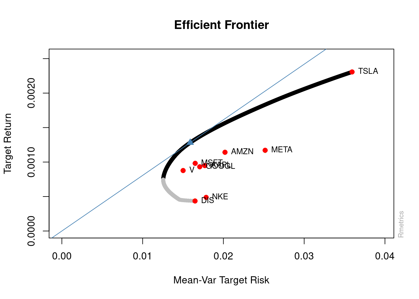
20.4.5 Identify the Optimal Weights
20.4.5.1 Tangency Portfolio
The tangency portfolio is the portfolio with the highest Sharpe ratio—i.e., the highest ratio of return to risk. In other words, it is the portfolio with the greatest risk-adjusted returns. We identify the tangency portfolio using the fPortfolio::tangencyPortfolio() function.
We extract the optimal weights for each asset at the tangency portfolio using the fPortfolio::getWeights() function.
Code
 AAPL.Close  MSFT.Close GOOGL.Close  AMZN.Close  META.Close     V.Close
0.146472865 0.004571997 0.216090167 0.097922481 0.030424447 0.311097639
  DIS.Close   NKE.Close  TSLA.Close
0.000000000 0.000000000 0.193420404
Title:
MV Tangency Portfolio
Estimator: covEstimator
Solver: solveRquadprog
Optimize: minRisk
Constraints: LongOnly
Portfolio Weights:
AAPL.Close MSFT.Close GOOGL.Close AMZN.Close META.Close V.Close
0.1465 0.0046 0.2161 0.0979 0.0304 0.3111
DIS.Close NKE.Close TSLA.Close
0.0000 0.0000 0.1934
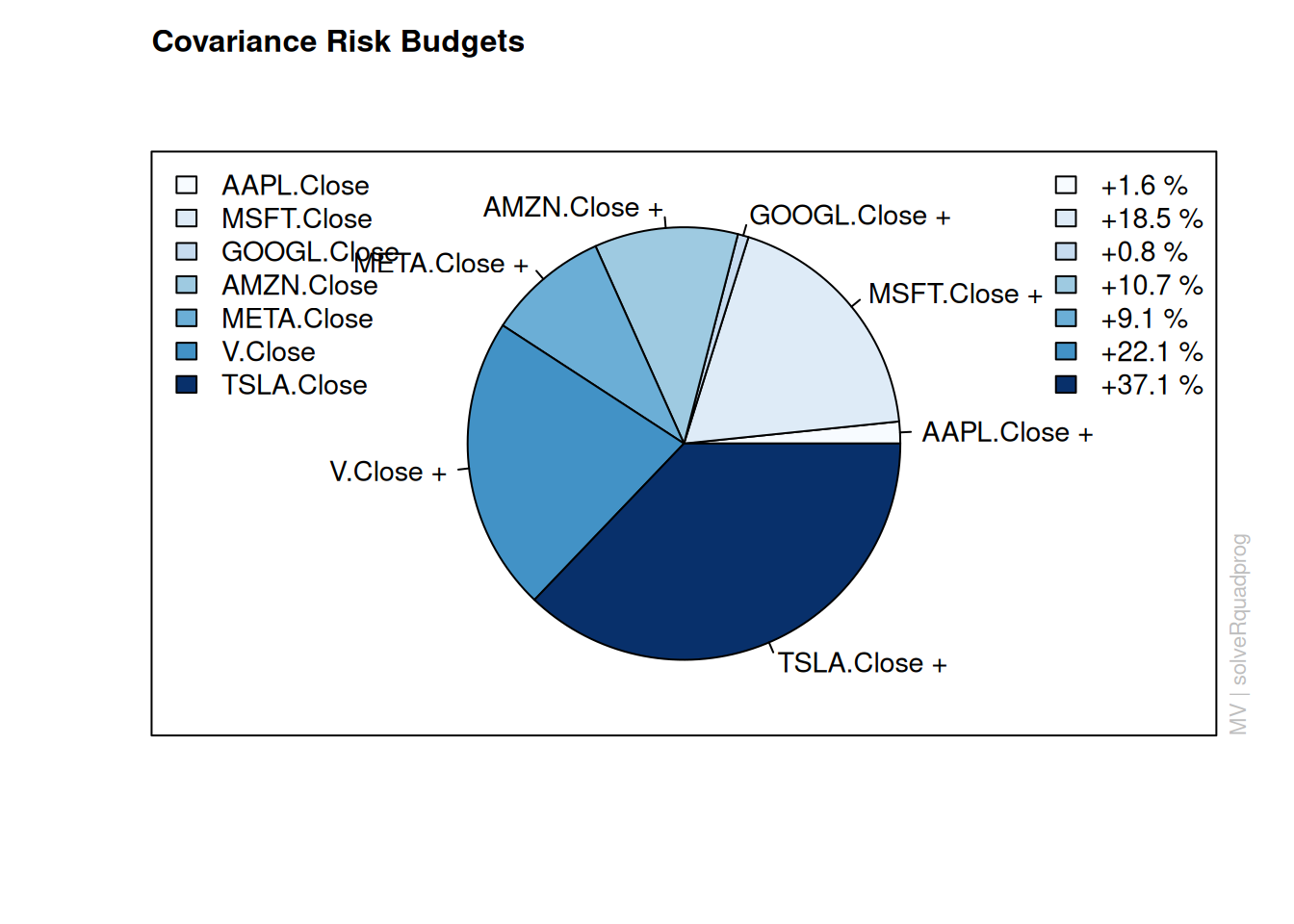
Covariance Risk Budgets:
AAPL.Close MSFT.Close GOOGL.Close AMZN.Close META.Close V.Close
0.1205 0.0034 0.1881 0.0904 0.0286 0.2200
DIS.Close NKE.Close TSLA.Close
0.0000 0.0000 0.3491
Target Returns and Risks:
mean Cov CVaR VaR
0.0012 0.0153 0.0349 0.0239
Description:
Fri Jul 24 16:56:55 2026 by user: 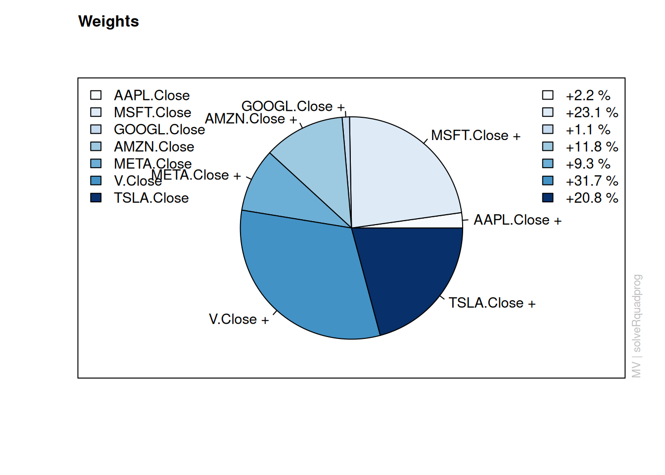

20.4.5.2 Portfolio with Max Return at a Given Risk Level
If the fPortfolio::maxreturnPortfolio() function worked as expected, the following could should work for determining the portfolio with the maximum return at each of various risk levels. However, there is a known bug in the fportfolio package (Wuertz et al., 2023) that the optimal portfolio (based on maximum returns) does not change when changing the target risk level, suggesting that it is not taking into account the target risk level specified by the user (see here: https://stackoverflow.com/q/78784306/2029527).
Code
# Define target risk levels
targetRisks <- seq(0, 0.3, by = 0.01)

# Initialize storage for optimal portfolios
optimalPortfolios <- list()
optimalWeights_list <- list()

# Find optimal weightings for each target risk level
for (risk in targetRisks) {
  # Create a portfolio optimization specification with the target risk
  portfolioSpec <- fPortfolio::portfolioSpec()
  fPortfolio::setTargetRisk(portfolioSpec) <- risk

  # Solve for the maximum return at this target risk
  optimal_portfolio <- fPortfolio::maxreturnPortfolio(
    returns_ts,
    spec = portfolioSpec)

  # Store the optimal portfolio
  optimalPortfolios[[as.character(risk)]] <- optimal_portfolio

  # Store the optimal portfolio weights with risk level
  optimal_weights <- fPortfolio::getWeights(optimal_portfolio)
  optimalWeights_list[[as.character(risk)]] <- c(RiskLevel = risk, optimal_weights)
}

optimalWeightsByRisk <- dplyr::bind_rows(optimalWeights_list)
optimalWeightsByRisk
20.5 The Efficient Frontier of a Fantasy Team
In fantasy football, the efficient frontier can be helpful for identifying the optimal players to draft for a given risk level (and potentially within the salary cap). It can also be helpful for identifying potential trades. In this way, modern portfolio theory and the efficient frontier can be helpful for arbitrage—buying and selling the same asset (in this case, player) to take advantage of different prices for the same asset. That is, you could buy low and, for players who outperform expectations, sell high—in the form of a trade.
20.5.1 Based on Variability Across Projection Sources
We can examine the efficient frontier of fantasy performance based on the mean and variability of players’ projected fantasy points across projection sources.
Code
all_proj_summary <- all_proj |>
  group_by(id) |>
  summarise(
    mean = mean(projectedPoints, na.rm = TRUE),
    sd = sd(projectedPoints, na.rm = TRUE),
    var = var(projectedPoints, na.rm = TRUE)
  )

all_proj_summary <- all_proj_summary |>
  left_join(
    nfl_playerIDs[,c("mfl_id","name","merge_name","position","team")],
    by = c("id" = "mfl_id")
  ) |>
  select(name, team, position, everything()) |>
  arrange(-mean)
As shown below, the correlation between mean and standard deviation of projected points is positive. That is, greater expected returns (i.e., mean of projected fantasy points) are associated with greater risk or volatility (i.e., standard deviation of projected fantasy points). Thus, to obtain a lineup that scores greater fantasy points, it may be necessary to take on greater risk. Moreover, you would not want take take on more risk for the same number of expected fantasy points; in addition, you would not want to score fewer fantasy points for the same amount of risk (Hitchings, 2012; archived at https://perma.cc/NE35-G6LR).
    Pearson's product-moment correlation

data:  mean and sd
t = 10.273, df = 995, p-value < 0.00000000000000022
alternative hypothesis: true correlation is not equal to 0
95 percent confidence interval:
 0.2524313 0.3647383
sample estimates:
      cor
0.3096644
A scatterplot of the expected returns versus risk, based on projected fantasy points, is in Figure 20.3.
Code
plot_projectedPointsMeanVsSD <- ggplot2::ggplot(
  data = all_proj_summary,
  aes(
    x = sd,
    y = mean)) +
  geom_point(
    aes(
      text = name, # add player name for mouse over tooltip
      label = position)) + # add season for mouse over tooltip
  #geom_smooth() +
  coord_cartesian(
    xlim = c(0,NA),
    ylim = c(0,NA),
    expand = FALSE) +
  labs(
    x = "Standard Deviation of Player's Projected Fantasy Points (Season) Across Sources",
    y = "Mean of Player's Projected Fantasy Points (Season) Across Sources",
    title = "Mean vs Standard Deviation of Players' Projected Fantasy Points"
  ) +
  theme_classic()

plotly::ggplotly(plot_projectedPointsMeanVsSD)Now let’s consider the expected returns versus risk for a combination of players. The formula for the variance (and standard deviation) of the sum of two variables is in Equation 20.1:
\[ \begin{aligned} \text{Var}(x + y) &= \text{Var}(x) + \text{Var}(y) + 2\text{Cov}(x, y)\\ s^2_{(x + y)} &= s^2_x + s^2_y + 2\text{Cov}(x, y)\\ \text{Std Dev}(x + y) &= \sqrt{\text{Var}(x) + \text{Var}(y) + 2\text{Cov}(x, y)}\\ s_{(x + y)} &= \sqrt{s^2_x + s^2_y + 2\text{Cov}(x, y)}\\ \end{aligned} \tag{20.1}\]
If we assume that players’ performance is uncorrelated with one another, the covariance between the players is zero, so the formula simplifies to Equation 20.2:
\[ \begin{aligned} \text{Var}(x + y) &= \text{Var}(x) + \text{Var}(y)\\ s^2_{(x + y)} &= s^2_x + s^2_y\\ \text{Std Dev}(x + y) &= \sqrt{\text{Var}(x) + \text{Var}(y)}\\ s_{(x + y)} &= \sqrt{s^2_x + s^2_y}\\ \end{aligned} \tag{20.2}\]
That is, if players’ performance is independent of each other, the variance of two players’ points is merely the sum of their variances; their standard deviation is then the square root of that. In reality, players’ performance is not truly independent—particularly for players on the same team or, for a given game, for players on opposing teams. However, for players not playing in the same game, it is a reasonable assumption to make and it greatly simplifies the math. If you wanted to, you could account for players’ covariance by using Equation 20.1. An example variance-covariance matrix of players’ performance is in Section 20.5.2.
Below is code for obtaining the expected returns and risk for various combinations of Quarterback, Running Back, and Wide Receiver.
Code
hiLo_permutations <- expand.grid(
  rep(list(c("Hi", "Lo")), 3),
  stringsAsFactors = FALSE
)

qbRbWr_projections <- data.frame(
  condition = c("Hi", "Lo"),
  qb_name = c("Josh Allen", "Matthew Stafford"),
  rb_name = c("Saquon Barkley", "Joe Mixon"),
  wr_name = c("Ja'Marr Chase", "Courtland Sutton")
)

qbRbWr_projections$qb_mean <- c(
  all_proj_summary$mean[which(all_proj_summary$position == "QB" & all_proj_summary$name == qbRbWr_projections$qb_name[1])],
  all_proj_summary$mean[which(all_proj_summary$position == "QB" & all_proj_summary$name == qbRbWr_projections$qb_name[2])])

qbRbWr_projections$qb_sd <- c(
  all_proj_summary$sd[which(all_proj_summary$position == "QB" & all_proj_summary$name == qbRbWr_projections$qb_name[1])],
  all_proj_summary$sd[which(all_proj_summary$position == "QB" & all_proj_summary$name == qbRbWr_projections$qb_name[2])])

qbRbWr_projections$rb_mean <- c(
  all_proj_summary$mean[which(all_proj_summary$position == "RB" & all_proj_summary$name == qbRbWr_projections$rb_name[1])],
  all_proj_summary$mean[which(all_proj_summary$position == "RB" & all_proj_summary$name == qbRbWr_projections$rb_name[2])])

qbRbWr_projections$rb_sd <- c(
  all_proj_summary$sd[which(all_proj_summary$position == "RB" & all_proj_summary$name == qbRbWr_projections$rb_name[1])],
  all_proj_summary$sd[which(all_proj_summary$position == "RB" & all_proj_summary$name == qbRbWr_projections$rb_name[2])])

qbRbWr_projections$wr_mean <- c(
  all_proj_summary$mean[which(all_proj_summary$position == "WR" & all_proj_summary$name == qbRbWr_projections$wr_name[1])],
  all_proj_summary$mean[which(all_proj_summary$position == "WR" & all_proj_summary$name == qbRbWr_projections$wr_name[2])])

qbRbWr_projections$wr_sd <- c(
  all_proj_summary$sd[which(all_proj_summary$position == "WR" & all_proj_summary$name == qbRbWr_projections$wr_name[1])],
  all_proj_summary$sd[which(all_proj_summary$position == "WR" & all_proj_summary$name == qbRbWr_projections$wr_name[2])])

qbRbWr_projections$qb_lastName <- sapply(strsplit(qbRbWr_projections$qb_name, " "), function(x) tail(x, 1))
qbRbWr_projections$rb_lastName <- sapply(strsplit(qbRbWr_projections$rb_name, " "), function(x) tail(x, 1))
qbRbWr_projections$wr_lastName <- sapply(strsplit(qbRbWr_projections$wr_name, " "), function(x) tail(x, 1))

team_projections <- data.frame(
  team = apply(hiLo_permutations, 1, paste0, collapse = ""),
  team_name = NA,
  team_mean = NA,
  team_sd = NA,
  qb = hiLo_permutations$Var1,
  rb = hiLo_permutations$Var2,
  wr = hiLo_permutations$Var3,
  qb_name = NA,
  qb_lastName = NA,
  qb_mean = NA,
  qb_sd = NA,
  rb_name = NA,
  rb_lastName = NA,
  rb_mean = NA,
  rb_sd = NA,
  wr_name = NA,
  wr_lastName = NA,
  wr_mean = NA,
  wr_sd = NA
)

team_projections$qb_name[which(team_projections$qb == "Hi")] <- qbRbWr_projections$qb_name[which(qbRbWr_projections$condition == "Hi")]
team_projections$qb_name[which(team_projections$qb == "Lo")] <- qbRbWr_projections$qb_name[which(qbRbWr_projections$condition == "Lo")]
team_projections$qb_lastName[which(team_projections$qb == "Hi")] <- qbRbWr_projections$qb_lastName[which(qbRbWr_projections$condition == "Hi")]
team_projections$qb_lastName[which(team_projections$qb == "Lo")] <- qbRbWr_projections$qb_lastName[which(qbRbWr_projections$condition == "Lo")]
team_projections$qb_mean[which(team_projections$qb == "Hi")] <- qbRbWr_projections$qb_mean[which(qbRbWr_projections$condition == "Hi")]
team_projections$qb_mean[which(team_projections$qb == "Lo")] <- qbRbWr_projections$qb_mean[which(qbRbWr_projections$condition == "Lo")]
team_projections$qb_sd[which(team_projections$qb == "Hi")] <- qbRbWr_projections$qb_sd[which(qbRbWr_projections$condition == "Hi")]
team_projections$qb_sd[which(team_projections$qb == "Lo")] <- qbRbWr_projections$qb_sd[which(qbRbWr_projections$condition == "Lo")]

team_projections$rb_name[which(team_projections$rb == "Hi")] <- qbRbWr_projections$rb_name[which(qbRbWr_projections$condition == "Hi")]
team_projections$rb_name[which(team_projections$rb == "Lo")] <- qbRbWr_projections$rb_name[which(qbRbWr_projections$condition == "Lo")]
team_projections$rb_lastName[which(team_projections$rb == "Hi")] <- qbRbWr_projections$rb_lastName[which(qbRbWr_projections$condition == "Hi")]
team_projections$rb_lastName[which(team_projections$rb == "Lo")] <- qbRbWr_projections$rb_lastName[which(qbRbWr_projections$condition == "Lo")]
team_projections$rb_mean[which(team_projections$rb == "Hi")] <- qbRbWr_projections$rb_mean[which(qbRbWr_projections$condition == "Hi")]
team_projections$rb_mean[which(team_projections$rb == "Lo")] <- qbRbWr_projections$rb_mean[which(qbRbWr_projections$condition == "Lo")]
team_projections$rb_sd[which(team_projections$rb == "Hi")] <- qbRbWr_projections$rb_sd[which(qbRbWr_projections$condition == "Hi")]
team_projections$rb_sd[which(team_projections$rb == "Lo")] <- qbRbWr_projections$rb_sd[which(qbRbWr_projections$condition == "Lo")]

team_projections$wr_name[which(team_projections$wr == "Hi")] <- qbRbWr_projections$wr_name[which(qbRbWr_projections$condition == "Hi")]
team_projections$wr_name[which(team_projections$wr == "Lo")] <- qbRbWr_projections$wr_name[which(qbRbWr_projections$condition == "Lo")]
team_projections$wr_lastName[which(team_projections$wr == "Hi")] <- qbRbWr_projections$wr_lastName[which(qbRbWr_projections$condition == "Hi")]
team_projections$wr_lastName[which(team_projections$wr == "Lo")] <- qbRbWr_projections$wr_lastName[which(qbRbWr_projections$condition == "Lo")]
team_projections$wr_mean[which(team_projections$wr == "Hi")] <- qbRbWr_projections$wr_mean[which(qbRbWr_projections$condition == "Hi")]
team_projections$wr_mean[which(team_projections$wr == "Lo")] <- qbRbWr_projections$wr_mean[which(qbRbWr_projections$condition == "Lo")]
team_projections$wr_sd[which(team_projections$wr == "Hi")] <- qbRbWr_projections$wr_sd[which(qbRbWr_projections$condition == "Hi")]
team_projections$wr_sd[which(team_projections$wr == "Lo")] <- qbRbWr_projections$wr_sd[which(qbRbWr_projections$condition == "Lo")]

team_projections$team_name <- apply(
  team_projections[, c("qb_lastName", "rb_lastName", "wr_lastName")],
  1,
  paste,
  collapse = "/"
)

team_projections$team_mean <- rowSums(team_projections[,c("qb_mean","rb_mean","wr_mean")])
team_projections$team_sd <- rowSums(team_projections[,c("qb_sd","rb_sd","wr_sd")])
In Figure 20.4, we depict the combined mean of projected fantasy points for a Quarterback/Running Back/Wide Receiver combination as a function of the standard deviation of their projected fantasy points across sources.
Code
ggplot2::ggplot(
  data = team_projections,
  aes(
    x = team_sd,
    y = team_mean,
    label = team_name)) +
  geom_point() +
  ggrepel::geom_text_repel() +
  labs(
    x = "Standard Deviation of Players' Projected Fantasy Points (Season) Across Sources",
    y = "Mean of Players' Projected Fantasy Points (Season) Across Sources",
    title = "Mean vs Standard Deviation of Players' Projected Fantasy Points"
  ) +
  theme_classic()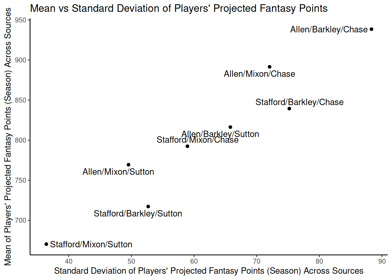
Now let’s generate the efficient frontier across all players.
Below, we use the NMOF::mvFrontier() function from the NMOF package (Gilli et al., 2019; Schumann, 2024a, 2024b) to compute the efficient frontier.
Code
const_cor <- function(rho, numAssets) {
C <- array(rho, dim = c(numAssets, numAssets))
diag(C) <- 1
C
}
varCovMatrix <- diag(all_proj_summary_noNA_removeZeroVar$sd) %*% const_cor(0, nrow(all_proj_summary_noNA_removeZeroVar)) %*% diag(all_proj_summary_noNA_removeZeroVar$sd) # create a variance-covariance matrix assuming assets/players are uncorrelated
efficientFrontierData <- NMOF::mvFrontier(
all_proj_summary_noNA_removeZeroVar$mean,
varCovMatrix,
wmin = 0,
wmax = 1,
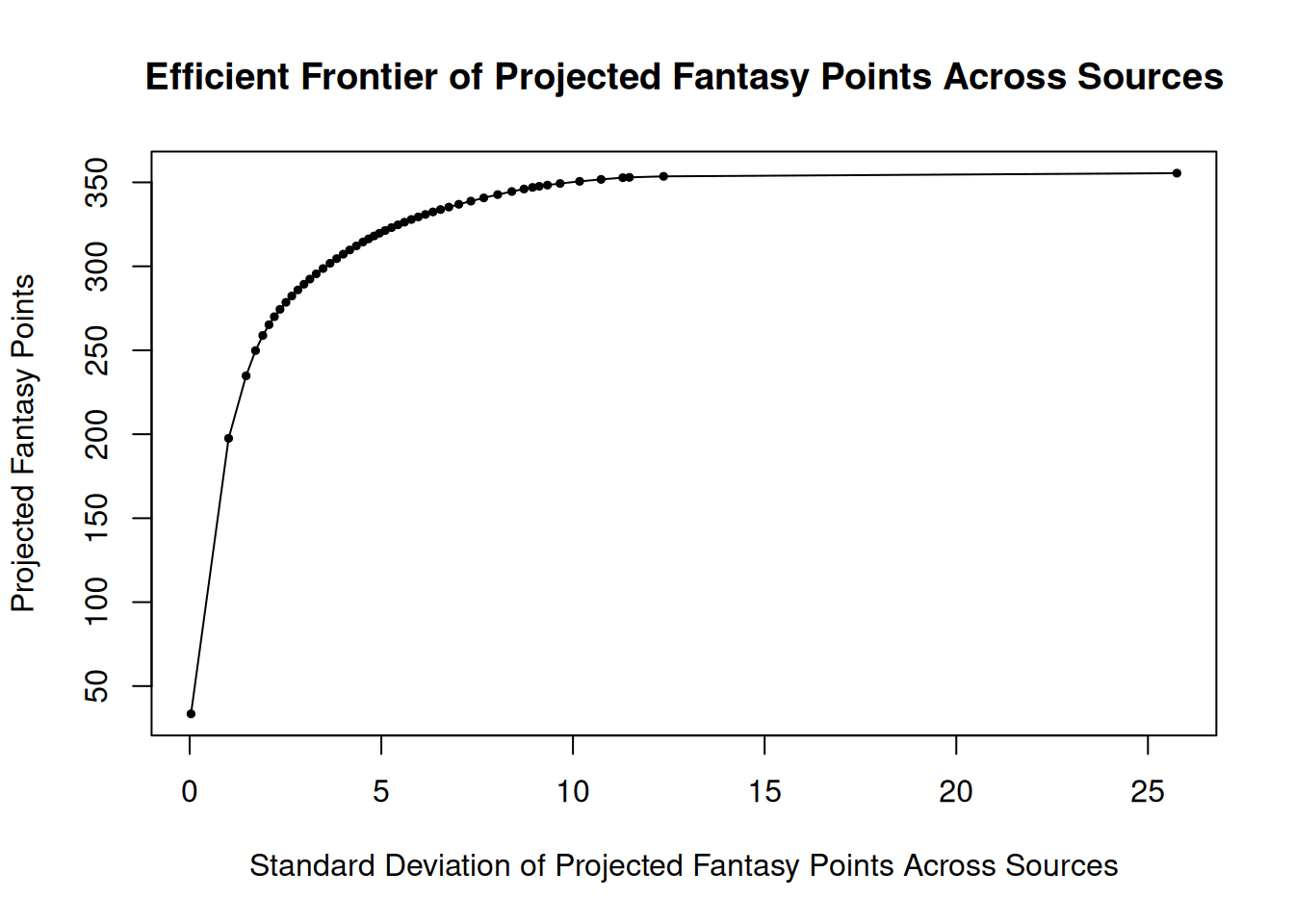
n = 50)When you evaluate all possible combinations of players, you can obtain the expected returns and standard deviations for each player combination. Based on that, you can determine the maximum number of fantasy points (i.e., the best possible team) at each level of risk. The best expected returns at each level of risk is known as the efficient frontier. The efficient frontier of projected fantasy points across sources is in Figure 20.5.
Code
20.5.2 Based on Historical Game-to-Game Variability
We can also examine the efficient frontier of fantasy performance based on the mean and variability of players’ historical (actual) week-to-week fantasy points (Hitchings, 2012; archived at https://perma.cc/JQ6G-KSRT).
Code
player_stats_weekly_recent <- player_stats_weekly |>
  filter(season == max(season))

player_stats_weekly_recent_summary <- player_stats_weekly_recent |>
  group_by(player_id) |>
  summarise(
    mean = mean(fantasyPoints, na.rm = TRUE),
    sd = sd(fantasyPoints, na.rm = TRUE),
    var = var(fantasyPoints, na.rm = TRUE)
  )

player_stats_weekly_recent_summary <- player_stats_weekly_recent_summary |>
  left_join(
    nfl_playerIDs[,c("gsis_id","name","merge_name","position","team")],
    by = c("player_id" = "gsis_id")
  ) |>
  select(name, team, position, everything()) |>
  arrange(-mean)
    Pearson's product-moment correlation

data:  mean and sd
t = 68.249, df = 1623, p-value < 0.00000000000000022
alternative hypothesis: true correlation is not equal to 0
95 percent confidence interval:
 0.8480452 0.8732203
sample estimates:
      cor
0.8611598
Here is the code to generate the variance-covariance matrix of players’ performance (it is very large because there are many players):
A scatterplot of the expected returns versus risk, based on weekly fantasy points, is in Figure 20.6.
Code
plot_fantasyPointsMeanVsSD <- ggplot2::ggplot(
  data = player_stats_weekly_recent_summary,
  aes(
    x = sd,
    y = mean)) +
  geom_point(
    aes(
      text = name, # add player name for mouse over tooltip
      label = position)) + # add season for mouse over tooltip
  #geom_smooth() +
  coord_cartesian(
    xlim = c(0,NA),
    ylim = c(0,NA),
    expand = FALSE) +
  labs(
    x = "Standard Deviation of Player's Fantasy Points From Week-to-Week",
    y = "Mean of Player's Fantasy Points Across Weeks",
    title = "Mean vs Standard Deviation of Players' Fantasy Points"
  ) +
  theme_classic()

plotly::ggplotly(plot_fantasyPointsMeanVsSD)Now let’s consider the expected returns versus risk for a combination of players. Below is code for obtaining the expected returns and risk for various combinations of Quarterback, Running Back, and Wide Receiver.
Code
qbRbWr_projections2 <- data.frame(
  condition = c("Hi", "Lo"),
  qb_name = c("Josh Allen", "Patrick Mahomes"),
  rb_name = c("Saquon Barkley", "David Montgomery"),
  wr_name = c("Ja'Marr Chase", "Stefon Diggs")
)

qbRbWr_projections2$qb_mean <- c(
  player_stats_weekly_recent_summary$mean[which(player_stats_weekly_recent_summary$position == "QB" & player_stats_weekly_recent_summary$name == qbRbWr_projections2$qb_name[1])],
  player_stats_weekly_recent_summary$mean[which(player_stats_weekly_recent_summary$position == "QB" & player_stats_weekly_recent_summary$name == qbRbWr_projections2$qb_name[2])])

qbRbWr_projections2$qb_sd <- c(
  player_stats_weekly_recent_summary$sd[which(player_stats_weekly_recent_summary$position == "QB" & player_stats_weekly_recent_summary$name == qbRbWr_projections2$qb_name[1])],
  player_stats_weekly_recent_summary$sd[which(player_stats_weekly_recent_summary$position == "QB" & player_stats_weekly_recent_summary$name == qbRbWr_projections2$qb_name[2])])

qbRbWr_projections2$rb_mean <- c(
  player_stats_weekly_recent_summary$mean[which(player_stats_weekly_recent_summary$position == "RB" & player_stats_weekly_recent_summary$name == qbRbWr_projections2$rb_name[1])],
  player_stats_weekly_recent_summary$mean[which(player_stats_weekly_recent_summary$position == "RB" & player_stats_weekly_recent_summary$name == qbRbWr_projections2$rb_name[2])])

qbRbWr_projections2$rb_sd <- c(
  player_stats_weekly_recent_summary$sd[which(player_stats_weekly_recent_summary$position == "RB" & player_stats_weekly_recent_summary$name == qbRbWr_projections2$rb_name[1])],
  player_stats_weekly_recent_summary$sd[which(player_stats_weekly_recent_summary$position == "RB" & player_stats_weekly_recent_summary$name == qbRbWr_projections2$rb_name[2])])

qbRbWr_projections2$wr_mean <- c(
  player_stats_weekly_recent_summary$mean[which(player_stats_weekly_recent_summary$position == "WR" & player_stats_weekly_recent_summary$name == qbRbWr_projections2$wr_name[1])],
  player_stats_weekly_recent_summary$mean[which(player_stats_weekly_recent_summary$position == "WR" & player_stats_weekly_recent_summary$name == qbRbWr_projections2$wr_name[2])])

qbRbWr_projections2$wr_sd <- c(
  player_stats_weekly_recent_summary$sd[which(player_stats_weekly_recent_summary$position == "WR" & player_stats_weekly_recent_summary$name == qbRbWr_projections2$wr_name[1])],
  player_stats_weekly_recent_summary$sd[which(player_stats_weekly_recent_summary$position == "WR" & player_stats_weekly_recent_summary$name == qbRbWr_projections2$wr_name[2])])

qbRbWr_projections2$qb_lastName <- sapply(strsplit(qbRbWr_projections2$qb_name, " "), function(x) tail(x, 1))
qbRbWr_projections2$rb_lastName <- sapply(strsplit(qbRbWr_projections2$rb_name, " "), function(x) tail(x, 1))
qbRbWr_projections2$wr_lastName <- sapply(strsplit(qbRbWr_projections2$wr_name, " "), function(x) tail(x, 1))

team_projections2 <- data.frame(
  team = apply(hiLo_permutations, 1, paste0, collapse = ""),
  team_name = NA,
  team_mean = NA,
  team_sd = NA,
  qb = hiLo_permutations$Var1,
  rb = hiLo_permutations$Var2,
  wr = hiLo_permutations$Var3,
  qb_name = NA,
  qb_lastName = NA,
  qb_mean = NA,
  qb_sd = NA,
  rb_name = NA,
  rb_lastName = NA,
  rb_mean = NA,
  rb_sd = NA,
  wr_name = NA,
  wr_lastName = NA,
  wr_mean = NA,
  wr_sd = NA
)

team_projections2$qb_name[which(team_projections2$qb == "Hi")] <- qbRbWr_projections2$qb_name[which(qbRbWr_projections2$condition == "Hi")]
team_projections2$qb_name[which(team_projections2$qb == "Lo")] <- qbRbWr_projections2$qb_name[which(qbRbWr_projections2$condition == "Lo")]
team_projections2$qb_lastName[which(team_projections2$qb == "Hi")] <- qbRbWr_projections2$qb_lastName[which(qbRbWr_projections2$condition == "Hi")]
team_projections2$qb_lastName[which(team_projections2$qb == "Lo")] <- qbRbWr_projections2$qb_lastName[which(qbRbWr_projections2$condition == "Lo")]
team_projections2$qb_mean[which(team_projections2$qb == "Hi")] <- qbRbWr_projections2$qb_mean[which(qbRbWr_projections2$condition == "Hi")]
team_projections2$qb_mean[which(team_projections2$qb == "Lo")] <- qbRbWr_projections2$qb_mean[which(qbRbWr_projections2$condition == "Lo")]
team_projections2$qb_sd[which(team_projections2$qb == "Hi")] <- qbRbWr_projections2$qb_sd[which(qbRbWr_projections2$condition == "Hi")]
team_projections2$qb_sd[which(team_projections2$qb == "Lo")] <- qbRbWr_projections2$qb_sd[which(qbRbWr_projections2$condition == "Lo")]

team_projections2$rb_name[which(team_projections2$rb == "Hi")] <- qbRbWr_projections2$rb_name[which(qbRbWr_projections2$condition == "Hi")]
team_projections2$rb_name[which(team_projections2$rb == "Lo")] <- qbRbWr_projections2$rb_name[which(qbRbWr_projections2$condition == "Lo")]
team_projections2$rb_lastName[which(team_projections2$rb == "Hi")] <- qbRbWr_projections2$rb_lastName[which(qbRbWr_projections2$condition == "Hi")]
team_projections2$rb_lastName[which(team_projections2$rb == "Lo")] <- qbRbWr_projections2$rb_lastName[which(qbRbWr_projections2$condition == "Lo")]
team_projections2$rb_mean[which(team_projections2$rb == "Hi")] <- qbRbWr_projections2$rb_mean[which(qbRbWr_projections2$condition == "Hi")]
team_projections2$rb_mean[which(team_projections2$rb == "Lo")] <- qbRbWr_projections2$rb_mean[which(qbRbWr_projections2$condition == "Lo")]
team_projections2$rb_sd[which(team_projections2$rb == "Hi")] <- qbRbWr_projections2$rb_sd[which(qbRbWr_projections2$condition == "Hi")]
team_projections2$rb_sd[which(team_projections2$rb == "Lo")] <- qbRbWr_projections2$rb_sd[which(qbRbWr_projections2$condition == "Lo")]

team_projections2$wr_name[which(team_projections2$wr == "Hi")] <- qbRbWr_projections2$wr_name[which(qbRbWr_projections2$condition == "Hi")]
team_projections2$wr_name[which(team_projections2$wr == "Lo")] <- qbRbWr_projections2$wr_name[which(qbRbWr_projections2$condition == "Lo")]
team_projections2$wr_lastName[which(team_projections2$wr == "Hi")] <- qbRbWr_projections2$wr_lastName[which(qbRbWr_projections2$condition == "Hi")]
team_projections2$wr_lastName[which(team_projections2$wr == "Lo")] <- qbRbWr_projections2$wr_lastName[which(qbRbWr_projections2$condition == "Lo")]
team_projections2$wr_mean[which(team_projections2$wr == "Hi")] <- qbRbWr_projections2$wr_mean[which(qbRbWr_projections2$condition == "Hi")]
team_projections2$wr_mean[which(team_projections2$wr == "Lo")] <- qbRbWr_projections2$wr_mean[which(qbRbWr_projections2$condition == "Lo")]
team_projections2$wr_sd[which(team_projections2$wr == "Hi")] <- qbRbWr_projections2$wr_sd[which(qbRbWr_projections2$condition == "Hi")]
team_projections2$wr_sd[which(team_projections2$wr == "Lo")] <- qbRbWr_projections2$wr_sd[which(qbRbWr_projections2$condition == "Lo")]

team_projections2$team_name <- apply(
  team_projections2[, c("qb_lastName", "rb_lastName", "wr_lastName")],
  1,
  paste,
  collapse = "/"
)

team_projections2$team_mean <- rowSums(team_projections2[,c("qb_mean","rb_mean","wr_mean")])
team_projections2$team_sd <- rowSums(team_projections2[,c("qb_sd","rb_sd","wr_sd")])
In Figure 20.7, we depict the combined mean of historical fantasy points for a Quarterback/Running Back/Wide Receiver combination as a function of the historical standard deviation of their fantasy points across games.
Code
ggplot2::ggplot(
  data = team_projections2,
  aes(
    x = team_sd,
    y = team_mean,
    label = team_name)) +
  geom_point() +
  ggrepel::geom_text_repel() +
  labs(
    x = "Standard Deviation of Players' Fantasy Points From Week-to-Week",
    y = "Mean of Players' Fantasy Points Across Weeks",
    title = "Mean vs Standard Deviation of Players' Actual Fantasy Points"
  ) +
  theme_classic()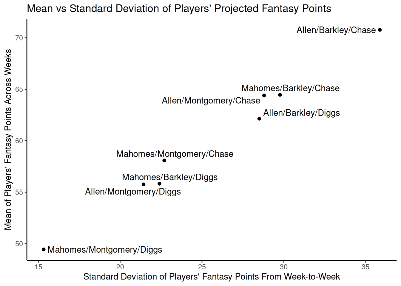
Now let’s generate the efficient frontier across all players.
Below, we use the NMOF::mvFrontier() function from the NMOF package (Gilli et al., 2019; Schumann, 2024a, 2024b) to compute the efficient frontier.
Code
varCovMatrix2 <- diag(player_stats_weekly_recent_summary_noNA_removeZeroVar$sd) %*% const_cor(0, nrow(player_stats_weekly_recent_summary_noNA_removeZeroVar)) %*% diag(player_stats_weekly_recent_summary_noNA_removeZeroVar$sd) # create a variance-covariance matrix assuming assets/players are uncorrelated
efficientFrontierData2 <- NMOF::mvFrontier(
player_stats_weekly_recent_summary_noNA_removeZeroVar$mean,
varCovMatrix2,
wmin = 0,
wmax = 1,
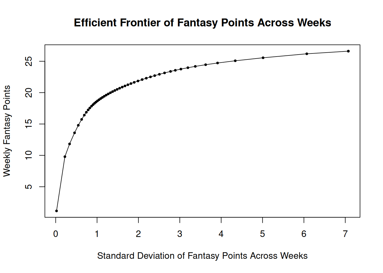
n = 50)The efficient frontier of fantasy points across weeks is in Figure 20.8.
Code
In these examples, we have computed the efficient frontier across all players. However, it would be more relevant to establish the efficient frontier for the possible combinations of players (e.g., one Quarterback, two Running Backs, two Wide Receivers, one Tight End, one Kicker, etc.). Nevertheless, the above examples illustrate how one might do this; one could extend the examples to consider whole teams rather than just three players at a time.
20.6 Conclusion
In summary, fantasy football is similar to stock picking. You are most likely to pick the best players if you go with the wisdom of the crowd (e.g., average projections across projection sources) and diversify. Players—like stocks—have expected returns and risk associated with them. You can think of constructing your team like constructing a stock portfolio, where your goal is to gain the maximum expected returns for a given level of risk. The greater risk you are willing to take, the greater the potential returns, but also the lower the potential downside if the players underperform. Thus, you may want your team to be composed of a diverse combination of some higher risk players and some lower risk players. We demonstrate the efficient frontier as a valuable tool for identifying the combination of players with the maximum expected returns relative to their risk. Most projections are public information, so you might wonder whether using crowd projections gains you anything because everybody else has access to public information. However, this is also the case with stocks, and people still consistently perform best over time when they go with the market. Nevertheless, crowd projections are not highly accurate. And fantasy football is a game, so feel free to have fun and deviate from the crowd! However, you may be just as (if not more) likely to be wrong by deviating from the crowd.
20.7 Session Info
R version 4.6.1 (2026-06-24)
Platform: x86_64-pc-linux-gnu
Running under: Ubuntu 24.04.4 LTS

Matrix products: default
BLAS:   /usr/lib/x86_64-linux-gnu/openblas-pthread/libblas.so.3
LAPACK: /usr/lib/x86_64-linux-gnu/openblas-pthread/libopenblasp-r0.3.26.so;  LAPACK version 3.12.0

locale:
 [1] LC_CTYPE=C.UTF-8       LC_NUMERIC=C           LC_TIME=C.UTF-8
 [4] LC_COLLATE=C.UTF-8     LC_MONETARY=C.UTF-8    LC_MESSAGES=C.UTF-8
 [7] LC_PAPER=C.UTF-8       LC_NAME=C              LC_ADDRESS=C
[10] LC_TELEPHONE=C         LC_MEASUREMENT=C.UTF-8 LC_IDENTIFICATION=C

time zone: UTC
tzcode source: system (glibc)

attached base packages:
[1] stats     graphics  grDevices utils     datasets  methods   base

other attached packages:
 [1] lubridate_1.9.5     forcats_1.0.1       stringr_1.6.0
 [4] dplyr_1.2.1         purrr_1.2.2         readr_2.2.0
 [7] tidyr_1.3.2         tibble_3.3.1        tidyverse_2.0.0
[10] GGally_2.4.0        ggplot2_4.0.3       NMOF_2.11-0
[13] fPortfolio_4023.84  fAssets_4023.85     fBasics_4052.98
[16] timeSeries_4052.112 timeDate_4052.112   quantmod_0.4.29
[19] TTR_0.24.4          xts_0.14.2          zoo_1.8-15

loaded via a namespace (and not attached):
 [1] tidyselect_1.2.1    viridisLite_0.4.3   farver_2.1.2
 [4] S7_0.2.2            bitops_1.0-9        fastmap_1.2.0
 [7] RCurl_1.98-1.19     XML_3.99-0.23       digest_0.6.39
[10] timechange_0.4.0    lifecycle_1.0.5     mvnormtest_0.1-9-3
[13] Rsolnp_2.0.1        magrittr_2.0.5      kernlab_0.9-33
[16] compiler_4.6.1      rlang_1.3.0         tools_4.6.1
[19] igraph_2.3.3        yaml_2.3.12         data.table_1.18.4
[22] knitr_1.51          sn_2.1.3            labeling_0.4.3
[25] htmlwidgets_1.6.4   mnormt_2.1.2        curl_7.1.0
[28] RColorBrewer_1.1-3  withr_3.0.3         numDeriv_2016.8-1.1
[31] grid_4.6.1          stats4_4.6.1        future_1.75.0
[34] globals_0.19.1      scales_1.4.0        MASS_7.3-65
[37] cli_3.6.6           mvtnorm_1.4-2       rmarkdown_2.31
[40] Rglpk_0.6-5.1       generics_0.1.4      otel_0.2.0
[43] future.apply_1.20.2 robustbase_0.99-7   httr_1.4.8
[46] tzdb_0.5.0          energy_1.7-12       parallel_4.6.1
[49] vctrs_0.7.3         boot_1.3-32         jsonlite_2.0.0
[52] slam_0.1-56         hms_1.1.4           ggrepel_0.9.8
[55] listenv_1.0.0       crosstalk_1.2.2     rneos_0.4-1
[58] plotly_4.12.1       spatial_7.3-18      glue_1.8.1
[61] parallelly_1.48.0   DEoptimR_1.2-0      ggstats_0.13.0
[64] codetools_0.2-20    ecodist_2.1.3       stringi_1.8.7
[67] gtable_0.3.6        fMultivar_4031.84   quadprog_1.5-8
[70] gsl_2.1-9           pillar_1.11.1       htmltools_0.5.9
[73] truncnorm_1.0-9     R6_2.6.1            evaluate_1.0.5
[76] lattice_0.22-9      Rcpp_1.1.2          fCopulae_4052.86
[79] xfun_0.60           pkgconfig_2.0.3