I want your feedback to make the book better for you and other readers. If you find typos, errors, or places where the text may be improved, please let me know. The best ways to provide feedback are by GitHub or hypothes.is annotations.
You can leave a comment at the bottom of the page/chapter, or open an issue or submit a pull request on GitHub: https://github.com/isaactpetersen/Fantasy-Football-Analytics-Textbook
Alternatively, you can leave an annotation using hypothes.is.
To add an annotation, select some text and then click the
symbol on the pop-up menu.
To see the annotations of others, click the
symbol in the upper right-hand corner of the page.
24 Simulation: Bootstrapping and the Monte Carlo Method
This chapter provides an overview of various approaches to simulation, including bootstrapping and the Monte Carlo method.
24.1 Getting Started
24.1.1 Load Packages
24.1.2 Load Data
24.2 Overview
A simulation is an “imitative representation” of a phenomenon that could exist the real world. In statistics, simulations are computer-driven investigations to better understand a phenomenon by studying its behavior under different conditions. For instance, we might want to determine the likely range of outcomes for a player, in terms of the range of fantasy points that a player might score over the course of a season. Simulations can be conducted in various ways. Two common ways of conducting simulations are via bootstrapping and via Monte Carlo simulation.
24.2.1 Bootstrapping
Bootstrapping involves repeated resampling (with replacement) from observed data. For instance, if we have 100 sources provide projections for a player, we could estimate the most likely range of fantasy points for the player by repeatedly sampling from the 100 projections.
24.2.2 Monte Carlo Simulation
Monte Carlo simulation is named after the Casino de Monte-Carlo in Monaco because Monte Carlo simulations involve random samples (random chance), as might be found in casino gambling. Monte Carlo simulation involves repeated random sampling from a known distribution (Sigal & Chalmers, 2016). For instance, if we know the population distribution for the likely outcomes for a player—e.g., a normal distribution with a known mean (e.g., 150 points) and standard deviation (e.g., 20 points)—we can repeatedly sample randomly from this distribution. The distribution could be, as examples, a normal distribution, a log-normal distribution, a binomial distribution, a chi-square distribution, etc. (Sigal & Chalmers, 2016). The distribution provides a probability density function, which indicates the probability that any particular value would be observed if the data arose from that distribution.
24.3 Simulation of Projected Statistics and Points
Below, we perform bootstrapping and Monte Carlo simulations of projected statistics and points. However, it is worth noting that—as for any simulation—the quality of the results depend on the quality of the inputs. In this case, the quality of the simulation depends on the quality of the projections. If the projections are no good, the simulation results will not be trustworthy. Garbage in, garbage out. As we evaluated in Section 17.12, projections tend to show moderate accuracy for fantasy performance, but they are not highly accurate. Thus, we should treat simulation results arising from fantasy projections with a good dose of skepticism.
24.3.1 Bootstrapping
In this example, we simulate players’ likely distribution of (projected) fantasy points based on bootstrapping players’ projected statistics (e.g., passing yards, passing touchdowns). That is, for each iteration of the bootstrap, we randomly draw a projected value from a projection source (with replacement), for each of various statistical categories. For instance, assume we have 10 projection sources for Tom Brady. In iteration 1, we may draw Brady’s projected passing yards from ESPN and projected passing touchdowns from numberFire (i.e., randomly selected projection sources). In iteration 2, we may draw Brady’s projected passing yards from Yahoo and projected passing touchdowns from CBS (i.e., randomly selected projection sources). We do this for many iterations. We can compute projected fantasy points at each iteration and then summarize the distribution of fantasy points for Tom Brady (and all players) across all iterations.
This bootstrap simulation is valuable because it would give us a fuller distribution of the likely range of players’ performance than just the mean (or range) of projected points across sources. The simulated distribution provides information about our uncertainty of a player’s performance. For instance, using these distributions, we can then sample from the simulated distribution of likely fantasy points for each player to perform a simulation to identify the most optimal lineup across the simulation runs using our lineup optimizer (described in Section 7.4.2)
24.3.1.1 Prepare Data
Code
vars_by_pos <- list(
  QB = c(
    "games",
    "pass_att", "pass_comp", "pass_inc", "pass_yds", "pass_tds", "pass_int",
    "rush_att", "rush_yds", "rush_tds",
    "fumbles_lost", "fumbles_total", "two_pts",
    "sacks",
    "pass_09_tds", "pass_1019_tds", "pass_2029_tds", "pass_3039_tds", "pass_4049_tds", "pass_50_tds",
    "pass_40_yds", "pass_250_yds", "pass_300_yds", "pass_350_yds", "pass_400_yds",
    "rush_40_yds", "rush_50_yds", "rush_100_yds", "rush_150_yds", "rush_200_yds"
    ),
  RB = c(
    "games",
    "rush_att", "rush_yds", "rush_tds",
    "rec_tgt", "rec", "rec_yds", "rec_tds", "rec_rz_tgt",
    "fumbles_lost", "fumbles_total", "two_pts",
    "return_yds", "return_tds",
    "rush_09_tds", "rush_1019_tds", "rush_2029_tds", "rush_3039_tds", "rush_4049_tds", "rush_50_tds",
    "rush_40_yds", "rush_50_yds", "rush_100_yds", "rush_150_yds", "rush_200_yds",
    "rec_40_yds", "rec_50_yds", "rec_100_yds", "rec_150_yds", "rec_200_yds"
  ),
  WR = c(
    "games",
    "pass_att", "pass_comp", "pass_inc", "pass_yds", "pass_tds", "pass_int",
    "rush_att", "rush_yds", "rush_tds",
    "rec_tgt", "rec", "rec_yds", "rec_tds", "rec_rz_tgt",
    "fumbles_lost", "fumbles_total", "two_pts",
    "return_yds", "return_tds",
    "rush_09_tds", "rush_1019_tds", "rush_2029_tds", "rush_3039_tds", "rush_4049_tds", "rush_50_tds",
    "rush_40_yds", "rush_50_yds", "rush_100_yds", "rush_150_yds", "rush_200_yds",
    "rec_40_yds", "rec_50_yds", "rec_100_yds", "rec_150_yds", "rec_200_yds"
  ),
  TE = c(
    "games",
    "pass_att", "pass_comp", "pass_inc", "pass_yds", "pass_tds", "pass_int",
    "rush_att", "rush_yds", "rush_tds",
    "rec_tgt", "rec", "rec_yds", "rec_tds", "rec_rz_tgt",
    "fumbles_lost", "fumbles_total", "two_pts",
    "return_yds", "return_tds",
    "rush_09_tds", "rush_1019_tds", "rush_2029_tds", "rush_3039_tds", "rush_4049_tds", "rush_50_tds",
    "rush_40_yds", "rush_50_yds", "rush_100_yds", "rush_150_yds", "rush_200_yds",
    "rec_40_yds", "rec_50_yds", "rec_100_yds", "rec_150_yds", "rec_200_yds"
  ),
  K = c(
    "fg_0019", "fg_2029", "fg_3039", "fg_4049", "fg_50", "fg_50_att",
    "fg_39", "fg_att_39", "fg_49", "fg_49_att",
    "fg", "fg_att", "fg_miss", "xp", "xp_att"
  ),
  D = c(
    "idp_solo", "idp_asst", "idp_sack", "idp_int", "idp_fum_force", "idp_fum_rec", "idp_pd", "idp_td", "idp_safety"
  ),
  DL = c(
    "idp_solo", "idp_asst", "idp_sack", "idp_int", "idp_fum_force", "idp_fum_rec", "idp_pd", "idp_td", "idp_safety"
  ),
  LB = c(
    "idp_solo", "idp_asst", "idp_sack", "idp_int", "idp_fum_force", "idp_fum_rec", "idp_pd", "idp_td", "idp_safety"
  ),
  DB = c(
    "idp_solo", "idp_asst", "idp_sack", "idp_int", "idp_fum_force", "idp_fum_rec", "idp_pd", "idp_td", "idp_safety"
  ),
  DST = c(
    "dst_fum_recvr", "dst_fum_rec", "dst_int", "dst_safety", "dst_sacks", "dst_td", "dst_blk",
    "dst_fumbles", "dst_tackles", "dst_yds_against", "dst_pts_against", "dst_pts_allowed", "dst_ret_yds"
  )
)
24.3.1.2 Bootstrapping Function
For performing the bootstrapping, we leverage the data.table (Barrett et al., 2025) (data.table::as.data.table(); data.table::data.table(); data.table::rbindlist()), future (Bengtsson, 2025a) (future::plan(); future::multisession()), and future.apply (Bengtsson, 2025b) (future.apply::future_lapply()) packages for speed (by using parallel processing) and memory efficiency. We use the progressr (Bengtsson, 2024) package (progressr::handlers(); progressr::with_progress(); progressr::progressor()) to create a progress bar.
Code
bootstrapSimulation <- function(
    projectedStats,
    vars_by_pos,
    n_iter = 10000,
    seed = NULL,
    progress = TRUE) {

  dt <- data.table::as.data.table(projectedStats) # use data.table for speed
  all_ids <- unique(dt$id)

  if (!is.null(seed)) set.seed(seed)

  future::plan(future::multisession) # parallelize tasks across multiple background R sessions using multiple cores to speed up simulation

  if (progress) progressr::handlers("txtprogressbar") # specify progress-bar style

  results <- progressr::with_progress({ # wrap in with_progress for progress bar
    p <- if (progress) progressr::progressor(along = all_ids) else NULL # create progressor for progress bar

    future.apply::future_lapply(
      all_ids, # apply the function below to each player using a parallelized loop
      function(player_id) {
        if (!is.null(p)) p() # advance progress bar

        player_data <- dt[id == player_id]
        player_pos  <- unique(player_data$pos)

        if (length(player_pos) != 1 || !player_pos %in% names(vars_by_pos)) return(NULL)

        stat_vars <- vars_by_pos[[player_pos]] # pull the relevant stat variables to simulate for this player's position
        out <- data.table(iteration = seq_len(n_iter), id = player_id, pos = player_pos)

        for (var in stat_vars) { # loop over each stat variable that should be simulated for the player's position
          if (var %in% names(player_data)) {
            non_na_values <- player_data[[var]][!is.na(player_data[[var]])] # pull non-missing values of the stat for the player (from all projection sources)

            if (length(non_na_values) > 0) {
              out[[var]] <- sample(non_na_values, n_iter, replace = TRUE) # if there are valid values, sample with replacement to simulate n_iter values
            } else {
              out[[var]] <- NA_real_ # specify a numeric missing value (if all values were missing)
            }
          } else {
            out[[var]] <- NA_real_ # specify a numeric missing value (if the stat variable doesn't exist)
          }
        }

        return(out)
      },
      future.seed = TRUE # ensures that each parallel process gets a reproducible random seed
    )
  })

  data.table::rbindlist(results, use.names = TRUE, fill = TRUE) # combines all the individual player results into one large data table, aligning columns by name; fill = TRUE ensures that missing columns are filled with NA where necessary
}
24.3.1.3 Run the Bootstrapping Simulation
24.3.1.4 Score Fantasy Points from the Simulation
Code
bootstrappedFantasyPoints$iteration <- bootstrappedFantasyPoints$data_src
bootstrappedFantasyPoints$data_src <- NULL

bootstrappedFantasyPoints <- bootstrappedFantasyPoints %>%
  left_join(
    nfl_playerIDs[,c("mfl_id","name","merge_name","team")],
    by = c("id" = "mfl_id")
  )

bootstrappedFantasyPoints <- bootstrappedFantasyPoints %>%
  rename(projectedPoints = raw_points)
24.3.1.5 Summarize Players’ Distribution of Projected Fantasy Points
Code
bootstrappedFantasyPoints_summary <- bootstrappedFantasyPoints %>%
  group_by(id) %>%
  summarise(
    mean = mean(projectedPoints, na.rm = TRUE),
    SD = sd(projectedPoints, na.rm = TRUE),
    min = min(projectedPoints, na.rm = TRUE),
    max = max(projectedPoints, na.rm = TRUE),
    q10 = quantile(projectedPoints, .10, na.rm = TRUE), # 10th quantile
    q90 = quantile(projectedPoints, .90, na.rm = TRUE), # 90th quantile
    range = max(projectedPoints, na.rm = TRUE) - min(projectedPoints, na.rm = TRUE),
    IQR = IQR(projectedPoints, na.rm = TRUE),
    MAD = mad(projectedPoints, na.rm = TRUE),
    CV = SD/mean,
    median = median(projectedPoints, na.rm = TRUE),
    pseudomedian = DescTools::HodgesLehmann(projectedPoints, na.rm = TRUE),
    mode = petersenlab::Mode(projectedPoints, multipleModes = "mean"),
    skewness = psych::skew(projectedPoints, na.rm = TRUE),
    kurtosis = psych::kurtosi(projectedPoints, na.rm = TRUE)
  )
24.3.1.6 View Players’ Distribution of Projected Fantasy Points
Code
Code
Code
Code
Code
Code
Code
Code
An example distribution of projected fantasy points is in Figure 24.1.
Code
ggplot2::ggplot(
  data = bootstrappedFantasyPoints %>%
    filter(pos == "QB" & name == "Patrick Mahomes"),
  mapping = aes(
    x = projectedPoints)
) +
  geom_histogram(
    aes(y = after_stat(density)),
    color = "#000000",
    fill = "#0099F8"
  ) +
  geom_density(
    color = "#000000",
    fill = "#F85700",
    alpha = 0.6 # add transparency
  ) +
  geom_rug() +
  #coord_cartesian(
  #  xlim = c(0,400)) +
  labs(
    x = "Fantasy Points",
    y = "Density",
    title = "Distribution of Projected Fantasy Points for Patrick Mahomes"
  ) +
  theme_classic() +
  theme(axis.title.y = element_text(angle = 0, vjust = 0.5)) # horizontal y-axis title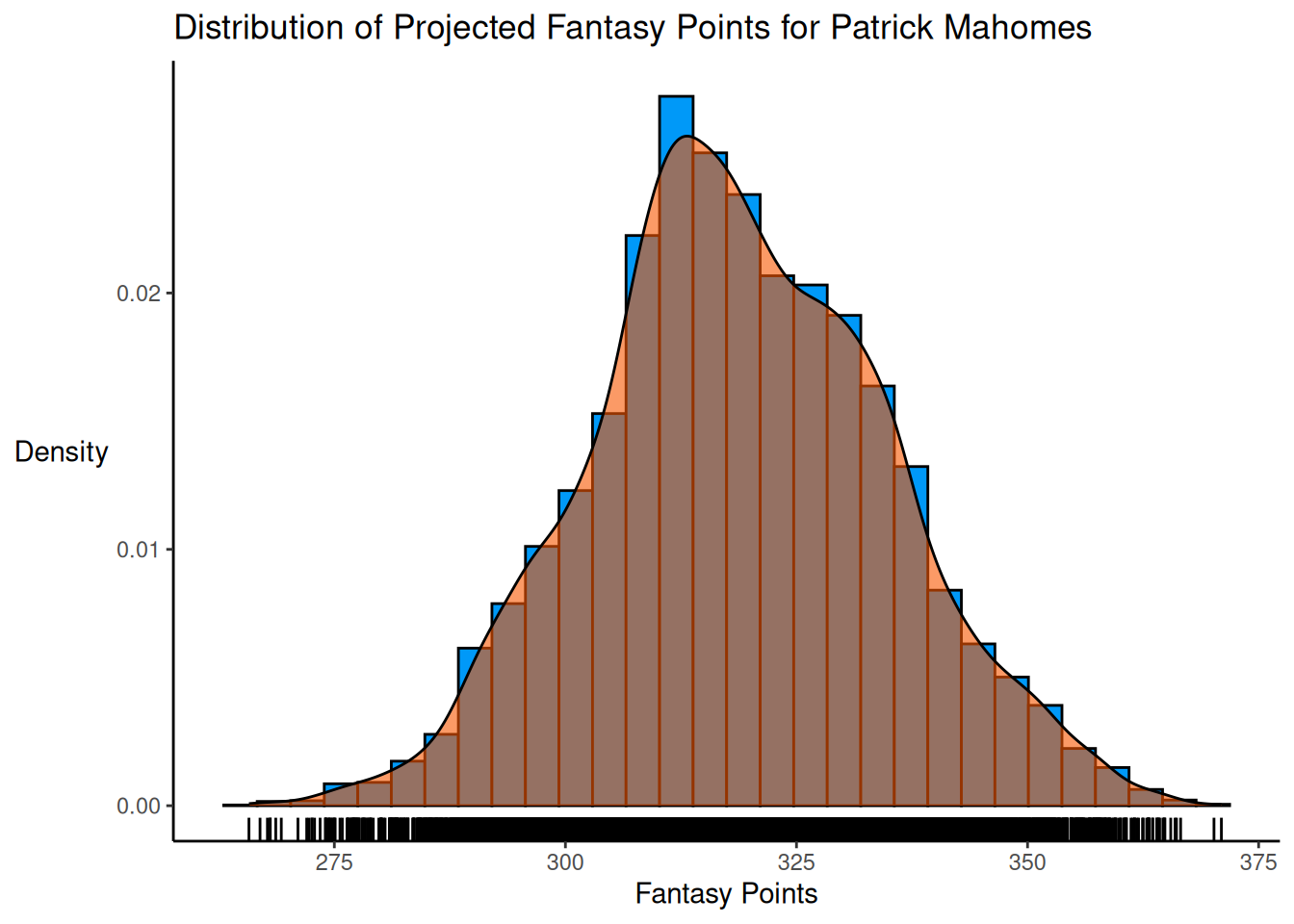
Projections of two players—one with relatively narrow uncertainty and one with relatively wide uncertainty—are depicted in Figure 24.2.
Code
ggplot2::ggplot(
  data = bootstrappedFantasyPoints %>%
    filter(pos == "QB" & (name %in% c("Dak Prescott", "Drake Maye"))),
  mapping = aes(
    x = projectedPoints,
    group = name,
    #color = name,
    fill = name)
) +
  geom_histogram(
    aes(y = after_stat(density))
  ) +
  geom_density(
    alpha = 0.6 # add transparency
  ) +
  coord_cartesian(
    xlim = c(0,NA),
    expand = FALSE) +
  #geom_rug() +
  labs(
    x = "Fantasy Points",
    y = "Density",
    fill = "",
    color = "",
    title = "Distribution of Projected Fantasy Points"
  ) +
  theme_classic() +
  theme(axis.title.y = element_text(angle = 0, vjust = 0.5)) # horizontal y-axis title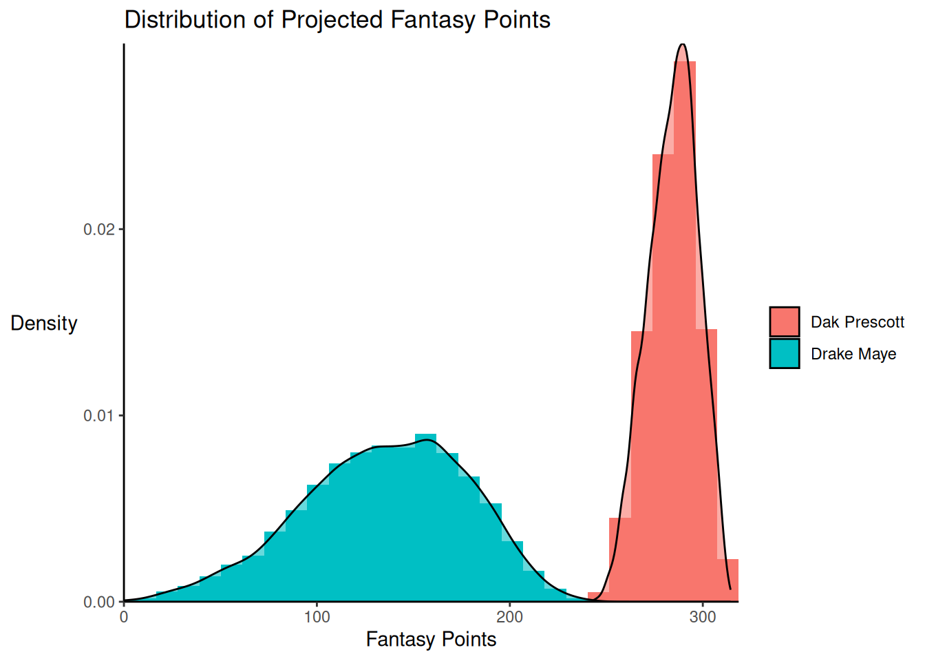
24.3.2 Monte Carlo Simulation
In general, a Monte Carlo simulation study involves several steps:
- generate the data for the simulation from the relevant probability distribution(s)
- analyze the simulated data
- summarize the results across the simulation replications
Below we conduct a Monte Carlo simulation to determine the range of each player’s most likely points scored based on their projected points. To do this, we use the SimDesign (Chalmers, 2025; Chalmers & Adkins, 2020) package.
24.3.2.1 SimDesign Package
The SimDesign (Chalmers, 2025; Chalmers & Adkins, 2020) package uses a five-step process to perform Monte Carlo simulations:
- Step 1—Design Grid: specify the fixed conditions to investigate in the simulation (e.g., sample size, generating distribution)
- Step 2—Generate: specify how to generate the data for the simulation from the relevant probability distribution(s)
- Step 3—Analyze: specify how to analyze the simulation data
- Step 4—Summarize: specify how to summarize the results across the simulation replications
- Step 5—Run the Simulation: run the simulation study (i.e., generate the data, analyze the simulated data, and summarize the results across the simulation replications)
You can generate a template for Monte Carlo simulations in the SimDesign (Chalmers, 2025; Chalmers & Adkins, 2020) package using the following code:
When designing a Monte Carlo simulation, Sigal & Chalmers (2016) (p. 151) recommend the following:
- beginning with a small number of replications and conditions (i.e., supplying a design object with fewer rows) to ensure that the code runs correctly, and increasing replications/conditions only when the majority of the bugs have been worked out
- documenting strange aspects of your simulation or code that you are likely to forget
- saving the state of your simulation in case of power failure or other mechanical failures (e.g., using the
save = TRUEand/orsave_results = TRUE, and/ordebugarguments inSimDesign::runSimulation()), and, as necessary, performing debugging within a particular function (debugargument inSimDesign::runSimulation())
24.3.2.2 Prepare Data
24.3.2.3 Optimal Distribution for Each Player
For each player, we identify the optimal distribution of their projected points across sources as either a normal distribution, or as a skew-normal distribution. The normal distribution was fit using the fitdistrplus::fitdist() function of the fitdistrplus package (Delignette-Muller & Dutang, 2015; Delignette-Muller et al., 2025). The skew-normal distribution was fit using the sn::selm() function of the sn package (A. Azzalini, 2023; A. A. Azzalini, 2023).
Code
# Function to identify the "best" distribution (Normal vs Skew‑Normal) for every player (tries both families and picks by AIC; uses empirical distribution if fewer than 2 unique scores)
fit_best <- function(x) {
  # Basic checks
  if (length(unique(x)) < 2 || all(is.na(x))) { # Use empirical distribution if there are fewer than 2 unique scores
    return(list(type = "empirical", empirical = x))
  }

  # Try Normal Distribution
  fit_norm <- tryCatch(
    fitdistrplus::fitdist(x, distr = "norm"),
    error = function(e) NULL
  )

  # Try Skew-Normal Distribution
  fit_skew <- tryCatch(
    sn::selm(x ~ 1),
    error = function(e) NULL
  )

  # Handle bad fits: sd = NA, etc.
  if (!is.null(fit_norm) && any(is.na(fit_norm$estimate))) {
    fit_norm <- NULL
  }

  if (!is.null(fit_skew)) {
    pars <- tryCatch(sn::coef(fit_skew, param.type = "dp"), error = function(e) NULL)
    if (is.null(pars) || any(is.na(pars))) {
      fit_skew <- NULL
    }
  }

  # Choose best available
  if (!is.null(fit_norm) && !is.null(fit_skew)) {
    aic_norm <- AIC(fit_norm)
    aic_skew <- AIC(fit_skew)
    if (aic_skew + 2 < aic_norm) { # skew-normal is more complex (has more parameters) than normal distribution, so only select a skew-normal distribution if it fits substantially better than a normal distribution
      pars <- sn::coef(fit_skew, param.type = "dp")
      return(list(
        type  = "skewnorm",
        xi    = pars["dp.location"],
        omega = pars["dp.scale"],
        alpha = pars["dp.shape"]))
    } else {
      return(list(
        type = "norm",
        mean = fit_norm$estimate["mean"],
        sd   = fit_norm$estimate["sd"]))
    }
  } else if (!is.null(fit_norm)) {
    return(list(
      type = "norm",
      mean = fit_norm$estimate["mean"],
      sd   = fit_norm$estimate["sd"]))
  } else {
    return(list(type = "empirical", empirical = x))
  }
}
Code
proj_dists_tbl <- all_proj %>%
  filter(!is.na(id) & id != "") %>%
  group_by(id) %>%
  summarise(
    dist_info = list(fit_best(projectedPoints)),
    n_proj = n(), # record of how many sources they have
    .groups = "drop"
  )

proj_dists <- proj_dists_tbl %>%
  filter(!is.na(id) & id != "") %>%
  distinct(id, .keep_all = TRUE) %>%
  (\(x) setNames(x$dist_info, x$id))()
24.3.2.4 SimDesign Step 1: Design Grid
First, we define what combinations of conditions to study (with one row per each unique combination), which is called our design grid. For the design grid, the columns are the design factors (e.g., sample size, generating distribution), and each row indicates a unique combination of the factors (e.g., N = 200, normal distribution; N = 500, normal distribution; N = 200, Poisson distribution; N = 500, Poisson distribution). When we execute the simulation, each row of the design grid object will be run sequentially.
In our simulation study, each player retains the same number of projections as they had in the original data, ensuring the simulation reflects real-world variation in data availability. This number of projections defines our design grid. The design factors (columns) are the player (id) and the number of projections available for that player (n_sources). The rows, then are the combinations of player and number of projections available for that player.
24.3.2.5 SimDesign Step 2: Generate
Second, we generate the data for the simulation from the relevant probability distribution function(s). In this case, we use a normal distribution or skew-normal distribution as our probability distribution function for a given player, depending on which distribution fits better to that player’s distribution of projected points across sources (stored in proj_dists[["INSERT_ID"]]$type). The Generate() function has a condition argument, which takes a single row from the design grid object (Design), and which controls the data generation for subsequent analysis. We use the (optional) fixed_objects argument so we can pass an object that should be held constant across all simulation replications—i.e., a “fixed” object. In this case, we pass—via the proj_dists object—the best-fitting distribution for each player (normal or skew-normal) to be used for all simulation replications.
Code
Generate <- function(condition, fixed_objects = NULL) {

  dist_info <- fixed_objects$proj_dists[[as.character(condition$id)]]
  n_sources <- condition$n_sources

  sim_points <- switch(
    dist_info$type,
    empirical = sample(
      dist_info$empirical,
      n_sources,
      replace = TRUE),

    norm = rnorm(
      n_sources,
      mean = dist_info$mean,
      sd = dist_info$sd),

    skewnorm = sn::rsn(
      n_sources,
      xi = dist_info$xi,
      omega = dist_info$omega,
      alpha = dist_info$alpha),

    stop("Unknown distribution type: ", dist_info$type)
  )

  data.frame(
    id = condition$id,
    sim_points = sim_points)
}
24.3.2.6 SimDesign Step 3: Analyze
Third, we analyze the simulated data. For each iteration of the simulation, the Analyse() function will return a vector with a requested variables: player (id), their simulated mean (mean_pts) and standard deviation (sd_pts) of projected fantasy points across sources, the 10th (q10) and 90th (q90) quartiles of their distributions of projected points, and the simulated probability of the player scoring at least 100 (p100), 150 (p150), 200 (p200), 250 (p250), 300 (p300), and 350 (p350) fantasy points. We then combine all the rows into a tibble dataframe, with each player as a different row. A separate dataset is created for each of the simulation replications.
Code
Analyse <- function(condition, dat, fixed_objects = NULL) {
  tibble::tibble(
    id        = condition$id,
    mean_pts  = mean(dat$sim_points, na.rm = TRUE),
    sd_pts    = sd(dat$sim_points, na.rm = TRUE),
    q10       = quantile(dat$sim_points, 0.10, na.rm = TRUE),
    q90       = quantile(dat$sim_points, 0.90, na.rm = TRUE),
    p100      = mean(dat$sim_points >= 100, na.rm = TRUE),
    p150      = mean(dat$sim_points >= 150, na.rm = TRUE),
    p200      = mean(dat$sim_points >= 200, na.rm = TRUE),
    p250      = mean(dat$sim_points >= 250, na.rm = TRUE),
    p300      = mean(dat$sim_points >= 300, na.rm = TRUE),
    p350      = mean(dat$sim_points >= 350, na.rm = TRUE)
  )
}
24.3.2.7 SimDesign Step 4: Summarize
Fourth, we summarize the results across the simulation replications. In this case, we calculate—for each variable—each player’s mean and standard deviation across the datasets from the different simulation replications.
Some potential metastatistics that can be computed include:
- mean:
base::mean() - standard deviation:
base::sd() - bias:
SimDesign::bias() - standardized bias:
SimDesign::bias(, type = "standardized") - relative bias:
SimDesign::bias(, type = "relative") - relative absolute bias:
SimDesign::RAB()orSimDesign::bias(, type = "abs_relative") - mean absolute error (MAE):
SimDesign::MAE() - normalized mean absolute error:
SimDesign::MAE(, type = "NMAE") - standardized mean absolute error:
SimDesign::MAE(, type = "SMAE") - root mean squared error (RMSE):
SimDesign::RMSE() - normalized root mean squared error:
SimDesign::RMSE(, type = "NRMSE") - standardized root mean squared error:
SimDesign::RMSE(, type = "SRMSE") - root mean squared log error (RMSLE):
SimDesign::RMSE(, type = "RMSLE") - integrated root mean squared error (IRMSE):
SimDesign::IRMSE() - mean-square relative standard error (MSRSE):
SimDesign::MSRSE() - coefficient of variation:
SimDesign::RMSE(, type = "CV") - relative efficiency:
SimDesign::RE() - empirical detection/rejection rate:
SimDesign::EDR() - empirical coverage rate:
SimDesign::ECR()
24.3.2.8 SimDesign Step 5: Run the Simulation
Fifth, we run the simulation study. We run the simulation study using the SimDesign::runSimulation() function.
Note: the following code that runs the simulation takes a while. If you just want to save time and load the results object instead of running the simulation, you can load the results object of the simulation (which has already been run) using this code:
Code
monteCarloSim_results <- SimDesign::runSimulation(
  design = Design,
  replications = 1000,
  generate = Generate,
  analyse = Analyse,
  summarise = Summarise,
  fixed_objects = list(proj_dists = proj_dists), # passing a list of objects that should be held constant across all simulation replications — i.e., "fixed" objects
  seed = SimDesign::genSeeds(Design, iseed = 52242), # for reproducibility
  parallel = TRUE # for faster (parallel) processing
)
24.3.2.9 Simulation Results
The pX variable represent the probability that a player scoring more than X number of points. For example, the p300 variable represents the probability that each player scores more than 300 points. However, it is important to note that this is based on the distribution of projected points.
24.4 Conclusion
A simulation is an “imitative representation” of a phenomenon that could exist the real world. In statistics, simulations are computer-driven investigations to better understand a phenomenon by studying its behavior under different conditions. Statistical simulations can be conducted in various ways. Two common types of simulations are bootstrapping and Monte Carlo simulation. Bootstrapping involves repeated resampling (with replacement) from observed data. Monte Carlo simulation involves repeated random sampling from a known distribution. We demonstrated bootstrapping and Monte Carlo approaches to simulating the most likely range of outcomes for a player in terms of fantasy points.
24.5 Session Info
R version 4.6.1 (2026-06-24)
Platform: x86_64-pc-linux-gnu
Running under: Ubuntu 24.04.4 LTS

Matrix products: default
BLAS:   /usr/lib/x86_64-linux-gnu/openblas-pthread/libblas.so.3
LAPACK: /usr/lib/x86_64-linux-gnu/openblas-pthread/libopenblasp-r0.3.26.so;  LAPACK version 3.12.0

locale:
 [1] LC_CTYPE=C.UTF-8       LC_NUMERIC=C           LC_TIME=C.UTF-8
 [4] LC_COLLATE=C.UTF-8     LC_MONETARY=C.UTF-8    LC_MESSAGES=C.UTF-8
 [7] LC_PAPER=C.UTF-8       LC_NAME=C              LC_ADDRESS=C
[10] LC_TELEPHONE=C         LC_MEASUREMENT=C.UTF-8 LC_IDENTIFICATION=C

time zone: UTC
tzcode source: system (glibc)

attached base packages:
[1] stats4    stats     graphics  grDevices utils     datasets  methods
[8] base

other attached packages:
 [1] lubridate_1.9.5         forcats_1.0.1           stringr_1.6.0
 [4] dplyr_1.2.1             purrr_1.2.2             readr_2.2.0
 [7] tidyr_1.3.2             tibble_3.3.1            ggplot2_4.0.3
[10] tidyverse_2.0.0         sn_2.1.3                fitdistrplus_1.2-6
[13] survival_3.8-6          MASS_7.3-65             SimDesign_2.25
[16] progressr_1.0.0         future.apply_1.20.2     future_1.70.0
[19] data.table_1.18.4       ffanalytics_3.1.15.0000

loaded via a namespace (and not attached):
  [1] RColorBrewer_1.1-3    rstudioapi_0.19.0     audio_0.1-12
  [4] jsonlite_2.0.0        magrittr_2.0.5        nloptr_2.2.1
  [7] farver_2.1.2          rmarkdown_2.31        fs_2.1.0
 [10] vctrs_0.7.3           minqa_1.2.8           base64enc_0.1-6
 [13] htmltools_0.5.9       haven_2.5.5           cellranger_1.1.0
 [16] Formula_1.2-5         parallelly_1.48.0     htmlwidgets_1.6.4
 [19] plyr_1.8.9            testthat_3.3.2        httr2_1.2.3
 [22] rootSolve_1.8.2.4     lifecycle_1.0.5       pkgconfig_2.0.3
 [25] Matrix_1.7-5          R6_2.6.1              fastmap_1.2.0
 [28] rbibutils_2.4.1       digest_0.6.39         Exact_3.3
 [31] numDeriv_2016.8-1.1   colorspace_2.1-3      ps_1.9.3
 [34] Hmisc_5.2-6           labeling_0.4.3        timechange_0.4.0
 [37] httr_1.4.8            compiler_4.6.1        proxy_0.4-29
 [40] withr_3.0.3           htmlTable_2.5.0       S7_0.2.2
 [43] backports_1.5.1       DBI_1.3.0             psych_2.6.5
 [46] R.utils_2.13.0        rappdirs_0.3.4        sessioninfo_1.2.4
 [49] petersenlab_1.2.3     gld_2.6.8             pbivnorm_0.6.0
 [52] tools_4.6.1           chromote_0.5.1        foreign_0.8-91
 [55] otel_0.2.0            clipr_0.8.1           nnet_7.3-20
 [58] R.oo_1.27.1           glue_1.8.1            quadprog_1.5-8
 [61] nlme_3.1-169          promises_1.5.0        grid_4.6.1
 [64] checkmate_2.3.4       reshape2_1.4.5        cluster_2.1.8.2
 [67] generics_0.1.4        gtable_0.3.6          tzdb_0.5.0
 [70] R.methodsS3_1.8.2     class_7.3-23          websocket_1.4.4
 [73] lmom_3.3              hms_1.1.4             xml2_1.6.0
 [76] stringfish_0.19.0     pillar_1.11.1         later_1.4.8
 [79] mitools_2.4           splines_4.6.1         lattice_0.22-9
 [82] tidyselect_1.2.1      pbapply_1.7-4         mix_1.0-13
 [85] knitr_1.51            reformulas_0.4.4      gridExtra_2.3.1
 [88] xfun_0.60             expm_1.0-0            brio_1.1.5
 [91] stringi_1.8.7         yaml_2.3.12           boot_1.3-32
 [94] evaluate_1.0.5        codetools_0.2-20      beepr_2.0
 [97] cli_3.6.6             RcppParallel_5.1.11-2 rpart_4.1.27
[100] xtable_1.8-8          Rdpack_2.6.6          DescTools_0.99.60
[103] processx_3.9.0        lavaan_0.6-21         mirai_2.7.1
[106] Rcpp_1.1.2            readxl_1.5.0          globals_0.19.1
[109] nanonext_1.10.1       parallel_4.6.1        lme4_2.0-1
[112] listenv_1.0.0         viridisLite_0.4.3     mvtnorm_1.4-2
[115] scales_1.4.0          e1071_1.7-17          rrapply_1.2.8
[118] rlang_1.3.0           qs2_0.2.2             rvest_1.0.5
[121] mnormt_2.1.2