I want your feedback to make the book better for you and other readers. If you find typos, errors, or places where the text may be improved, please let me know. The best ways to provide feedback are by GitHub or hypothes.is annotations.
You can leave a comment at the bottom of the page/chapter, or open an issue or submit a pull request on GitHub: https://github.com/isaactpetersen/Fantasy-Football-Analytics-Textbook
Alternatively, you can leave an annotation using hypothes.is.
To add an annotation, select some text and then click the
symbol on the pop-up menu.
To see the annotations of others, click the
symbol in the upper right-hand corner of the page.
10 Correlation Analysis
This chapter provides an overview of correlation analysis.
10.1 Getting Started
10.1.1 Load Packages
10.1.2 Load Data
We created the player_stats_weekly.RData and player_stats_seasonal.RData objects in Section 4.4.3.
10.2 Overview of Correlation
Correlation is an index of the association between variables. Covariance is the association between variables and in an unstandardized metric that differs for variables with different scales. By contrast, correlation is in a standardized metric that does not differ for variables with different scales. When examining the association between variables that are interval or ratio levels of measurement, Pearson correlation is used. When examining the association between variables that are ordinal in level of measurement, Spearman correlation is used. Pearson correlation is an index of the linear association between variables. If a nonlinear association is present, other indices like xi (\(\xi\); Chatterjee, 2021) and distance correlation coefficients are better suited to detect the association.
10.3 The Correlation Coefficient (\(r\))
The formula for the (Pearson) correlation coefficient is in Equation 9.28. As noted in Section 9.6.6, the correlation coefficient can be thought of as the ratio of shared variance (i.e., covariance) to total variance, as in Equation 9.30.
The correlation coefficient ranges from −1.0 to +1.0. The correlation coefficient (\(r\)) tells you two things: (1) the direction (sign) of the association (positive or negative) and (2) the magnitude of the association. If the correlation coefficient is positive, the association is positive. If the correlation coefficient is negative, the association is negative. If the association is positive, as X increases, Y increases (or conversely, as X decreases, Y decreases). If the association is negative, as X increases, Y decreases (or conversely, as X decreases, Y increases). The smaller the absolute value of the correlation coefficient (i.e., the closer the \(r\) value is to zero), the weaker the association and the flatter the standardized slope of the best-fit line in a scatterplot. The larger the absolute value of the correlation coefficient (i.e., the closer the absolute value of the \(r\) value is to one), the stronger the association and the steeper the standardized slope of the best-fit line. However, the correlation coefficient does not reflect the unstandardized slope of the best-fit line. See Figure 10.1 for a range of different correlation coefficients and what some example data may look like for each direction and strength of association.
Code
set.seed(52242)
correlations <- data.frame(criterion = rnorm(1000))
correlations$v1 <- complement(correlations$criterion, -1)
correlations$v2 <- complement(correlations$criterion, -.9)
correlations$v3 <- complement(correlations$criterion, -.8)
correlations$v4 <- complement(correlations$criterion, -.7)
correlations$v5 <- complement(correlations$criterion, -.6)
correlations$v6 <- complement(correlations$criterion, -.5)
correlations$v7 <- complement(correlations$criterion, -.4)
correlations$v8 <- complement(correlations$criterion, -.3)
correlations$v9 <- complement(correlations$criterion, -.2)
correlations$v10 <-complement(correlations$criterion, -.1)
correlations$v11 <-complement(correlations$criterion, 0)
correlations$v12 <-complement(correlations$criterion, .1)
correlations$v13 <-complement(correlations$criterion, .2)
correlations$v14 <-complement(correlations$criterion, .3)
correlations$v15 <-complement(correlations$criterion, .4)
correlations$v16 <-complement(correlations$criterion, .5)
correlations$v17 <-complement(correlations$criterion, .6)
correlations$v18 <-complement(correlations$criterion, .7)
correlations$v19 <-complement(correlations$criterion, .8)
correlations$v20 <-complement(correlations$criterion, .9)
correlations$v21 <-complement(correlations$criterion, 1)
par(mfrow = c(7,3), mar = c(1, 0, 1, 0))
# -1.0
plot(correlations$criterion, correlations$v1, xaxt = "n", yaxt = "n", xlab = "" , ylab = "",
main = substitute(paste(italic(r), " = ", x, sep = ""), list(x = round(cor.test(x = correlations$criterion, y = correlations$v1)$estimate, 2))))
abline(lm(v1 ~ criterion, data = correlations), col = "black")
# -.9
plot(correlations$criterion, correlations$v2, xaxt = "n", yaxt = "n", xlab = "" , ylab = "",
main = substitute(paste(italic(r), " = ", x, sep = ""), list(x = round(cor.test(x = correlations$criterion, y = correlations$v2)$estimate, 2))))
abline(lm(v2 ~ criterion, data = correlations), col = "black")
# -.8
plot(correlations$criterion, correlations$v3, xaxt = "n", yaxt = "n", xlab = "" , ylab = "",
main = substitute(paste(italic(r), " = ", x, sep = ""), list(x = round(cor.test(x = correlations$criterion, y = correlations$v3)$estimate, 2))))
abline(lm(v3 ~ criterion, data = correlations), col = "black")
# -.7
plot(correlations$criterion, correlations$v4, xaxt = "n", yaxt = "n", xlab = "" , ylab = "",
main = substitute(paste(italic(r), " = ", x, sep = ""), list(x = round(cor.test(x = correlations$criterion, y = correlations$v4)$estimate, 2))))
abline(lm(v4 ~ criterion, data = correlations), col = "black")
# -.6
plot(correlations$criterion, correlations$v5, xaxt = "n", yaxt = "n", xlab = "" , ylab = "",
main = substitute(paste(italic(r), " = ", x, sep = ""), list(x = round(cor.test(x = correlations$criterion, y = correlations$v5)$estimate, 2))))
abline(lm(v5 ~ criterion, data = correlations), col = "black")
# -.5
plot(correlations$criterion, correlations$v6, xaxt = "n", yaxt = "n", xlab = "" , ylab = "",
main = substitute(paste(italic(r), " = ", x, sep = ""), list(x = round(cor.test(x = correlations$criterion, y = correlations$v6)$estimate, 2))))
abline(lm(v6 ~ criterion, data = correlations), col = "black")
# -.4
plot(correlations$criterion, correlations$v7, xaxt = "n", yaxt = "n", xlab = "" , ylab = "",
main = substitute(paste(italic(r), " = ", x, sep = ""), list(x = round(cor.test(x = correlations$criterion, y = correlations$v7)$estimate, 2))))
abline(lm(v7 ~ criterion, data = correlations), col = "black")
# -.3
plot(correlations$criterion, correlations$v8, xaxt = "n", yaxt = "n", xlab = "" , ylab = "",
main = substitute(paste(italic(r), " = ", x, sep = ""), list(x = round(cor.test(x = correlations$criterion, y = correlations$v8)$estimate, 2))))
abline(lm(v8 ~ criterion, data = correlations), col = "black")
# -.2
plot(correlations$criterion, correlations$v9, xaxt = "n", yaxt = "n", xlab = "" , ylab = "",
main = substitute(paste(italic(r), " = ", x, sep = ""), list(x = round(cor.test(x = correlations$criterion, y = correlations$v9)$estimate, 2))))
abline(lm(v9 ~ criterion, data = correlations), col = "black")
# -.1
plot(correlations$criterion, correlations$v10, xaxt = "n", yaxt = "n", xlab = "" , ylab = "",
main = substitute(paste(italic(r), " = ", x, sep = ""), list(x = round(cor.test(x = correlations$criterion, y = correlations$v10)$estimate, 2))))
abline(lm(v10 ~ criterion, data = correlations), col = "black")
# 0.0
plot(correlations$criterion, correlations$v11, xaxt = "n", yaxt = "n", xlab = "" , ylab = "",
main = substitute(paste(italic(r), " = ", x, sep = ""), list(x = round(cor.test(x = correlations$criterion, y = correlations$v11)$estimate, 2))))
abline(lm(v11 ~ criterion, data = correlations), col = "black")
# 0.1
plot(correlations$criterion, correlations$v12, xaxt = "n", yaxt = "n", xlab = "" , ylab = "",
main = substitute(paste(italic(r), " = ", x, sep = ""), list(x = round(cor.test(x = correlations$criterion, y = correlations$v12)$estimate, 2))))
abline(lm(v12 ~ criterion, data = correlations), col = "black")
# 0.2
plot(correlations$criterion, correlations$v13, xaxt = "n", yaxt = "n", xlab = "" , ylab = "",
main = substitute(paste(italic(r), " = ", x, sep = ""), list(x = round(cor.test(x = correlations$criterion, y = correlations$v13)$estimate, 2))))
abline(lm(v13 ~ criterion, data = correlations), col = "black")
# 0.3
plot(correlations$criterion, correlations$v14, xaxt = "n", yaxt = "n", xlab = "" , ylab = "",
main = substitute(paste(italic(r), " = ", x, sep = ""), list(x = round(cor.test(x = correlations$criterion, y = correlations$v14)$estimate, 2))))
abline(lm(v14 ~ criterion, data = correlations), col = "black")
# 0.4
plot(correlations$criterion, correlations$v15, xaxt = "n", yaxt = "n", xlab = "" , ylab = "",
main = substitute(paste(italic(r), " = ", x, sep = ""), list(x = round(cor.test(x = correlations$criterion, y = correlations$v15)$estimate, 2))))
abline(lm(v15 ~ criterion, data = correlations), col = "black")
# 0.5
plot(correlations$criterion, correlations$v16, xaxt = "n", yaxt = "n", xlab = "" , ylab = "",
main = substitute(paste(italic(r), " = ", x, sep = ""), list(x = round(cor.test(x = correlations$criterion, y = correlations$v16)$estimate, 2))))
abline(lm(v16 ~ criterion, data = correlations), col = "black")
# 0.6
plot(correlations$criterion, correlations$v17, xaxt = "n", yaxt = "n", xlab = "" , ylab = "",
main = substitute(paste(italic(r), " = ", x, sep = ""), list(x = round(cor.test(x = correlations$criterion, y = correlations$v17)$estimate, 2))))
abline(lm(v17 ~ criterion, data = correlations), col = "black")
# 0.7
plot(correlations$criterion, correlations$v18, xaxt = "n", yaxt = "n", xlab = "" , ylab = "",
main = substitute(paste(italic(r), " = ", x, sep = ""), list(x = round(cor.test(x = correlations$criterion, y = correlations$v18)$estimate, 2))))
abline(lm(v18 ~ criterion, data = correlations), col = "black")
# 0.8
plot(correlations$criterion, correlations$v19, xaxt = "n", yaxt = "n", xlab = "" , ylab = "",
main = substitute(paste(italic(r), " = ", x, sep = ""), list(x = round(cor.test(x = correlations$criterion, y = correlations$v19)$estimate, 2))))
abline(lm(v19 ~ criterion, data = correlations), col = "black")
# 0.9
plot(correlations$criterion, correlations$v20, xaxt = "n", yaxt = "n", xlab = "" , ylab = "",
main = substitute(paste(italic(r), " = ", x, sep = ""), list(x = round(cor.test(x = correlations$criterion, y = correlations$v20)$estimate, 2))))
abline(lm(v20 ~ criterion, data = correlations), col = "black")
# 1.0
plot(correlations$criterion, correlations$v21, xaxt = "n", yaxt = "n", xlab = "" , ylab = "",
main = substitute(paste(italic(r), " = ", x, sep = ""), list(x = round(cor.test(x = correlations$criterion, y = correlations$v21)$estimate, 2))))
abline(lm(v21 ~ criterion, data = correlations), col = "black")
invisible(dev.off()) #par(mfrow = c(1,1))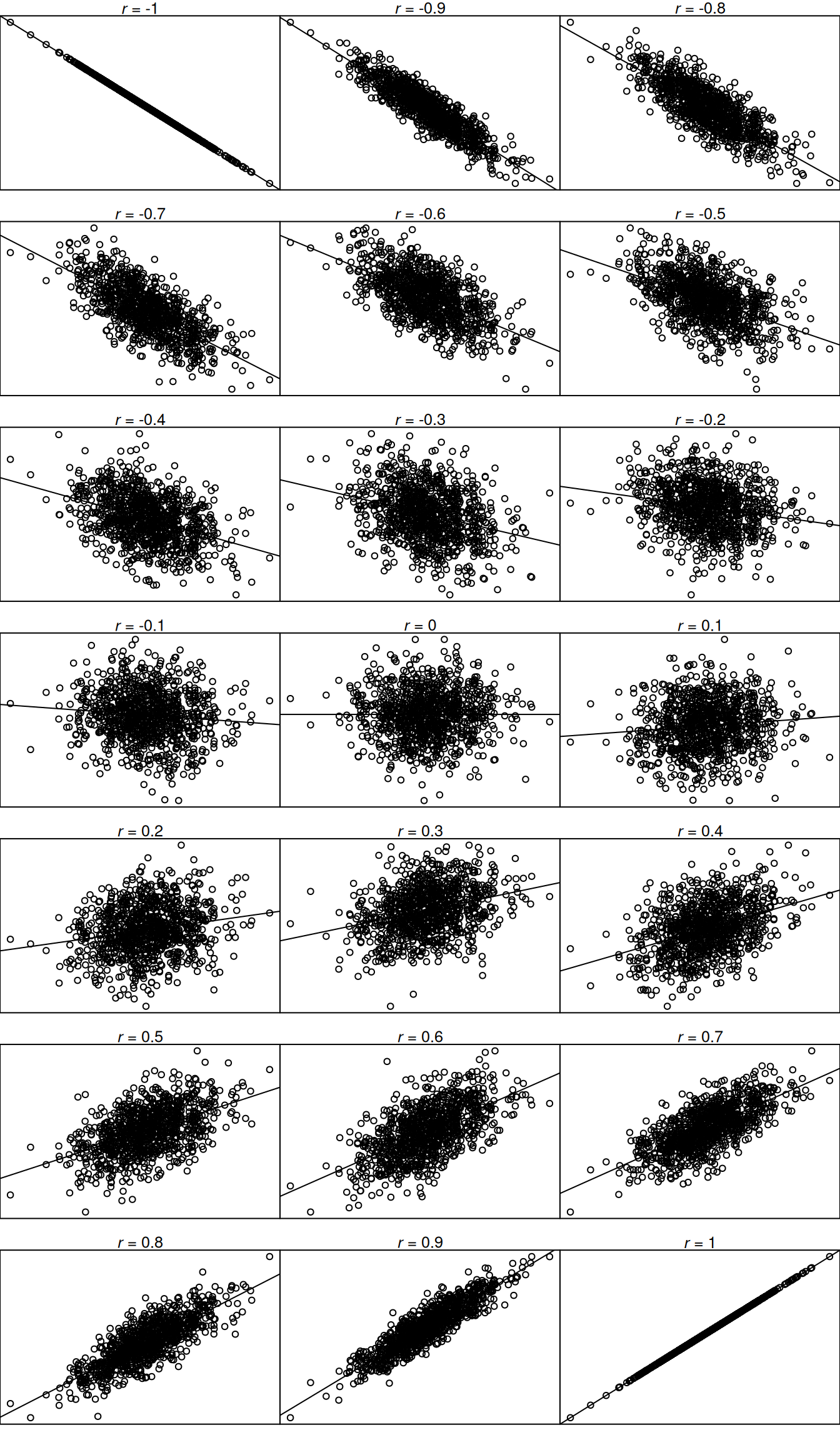
See Figure 10.2 for the interpretation of the magnitude and direction (sign) of various correlation coefficients.
Code
library("patchwork")
set.seed(52242)
correlations2 <- data.frame(criterion = rnorm(15))
correlations2$v1 <- complement(correlations2$criterion, -1)
correlations2$v2 <- complement(correlations2$criterion, -.9)
correlations2$v3 <- complement(correlations2$criterion, -.8)
correlations2$v4 <- complement(correlations2$criterion, -.7)
correlations2$v5 <- complement(correlations2$criterion, -.6)
correlations2$v6 <- complement(correlations2$criterion, -.5)
correlations2$v7 <- complement(correlations2$criterion, -.4)
correlations2$v8 <- complement(correlations2$criterion, -.3)
correlations2$v9 <- complement(correlations2$criterion, -.2)
correlations2$v10 <-complement(correlations2$criterion, -.1)
correlations2$v11 <-complement(correlations2$criterion, 0)
correlations2$v12 <-complement(correlations2$criterion, .1)
correlations2$v13 <-complement(correlations2$criterion, .2)
correlations2$v14 <-complement(correlations2$criterion, .3)
correlations2$v15 <-complement(correlations2$criterion, .4)
correlations2$v16 <-complement(correlations2$criterion, .5)
correlations2$v17 <-complement(correlations2$criterion, .6)
correlations2$v18 <-complement(correlations2$criterion, .7)
correlations2$v19 <-complement(correlations2$criterion, .8)
correlations2$v20 <-complement(correlations2$criterion, .9)
correlations2$v21 <-complement(correlations2$criterion, 1)
# -1.0
p1 <- ggplot(
data = correlations2,
mapping = aes(
x = criterion,
y = v1
)
) +
geom_point() +
geom_smooth(
method = "lm",
se = FALSE) +
labs(
title = "Perfect Negative Association",
subtitle = expression(paste(italic("r"), " = ", "−1.0"))
) +
theme_classic(
base_size = 12) +
theme(
axis.title.x = element_blank(),
axis.text.x = element_blank(),
axis.ticks.x = element_blank(),
axis.title.y = element_blank(),
axis.text.y = element_blank(),
axis.ticks.y = element_blank())
# -0.9
p2 <- ggplot(
data = correlations2,
mapping = aes(
x = criterion,
y = v2
)
) +
geom_point() +
geom_smooth(
method = "lm",
se = FALSE) +
labs(
title = "Strong Negative Association",
subtitle = expression(paste(italic("r"), " = ", "−.9"))
) +
theme_classic(
base_size = 12) +
theme(
axis.title.x = element_blank(),
axis.text.x = element_blank(),
axis.ticks.x = element_blank(),
axis.title.y = element_blank(),
axis.text.y = element_blank(),
axis.ticks.y = element_blank())
# -0.5
p3 <- ggplot(
data = correlations2,
mapping = aes(
x = criterion,
y = v6
)
) +
geom_point() +
geom_smooth(
method = "lm",
se = FALSE) +
labs(
title = "Moderate Negative Association",
subtitle = expression(paste(italic("r"), " = ", "−.5"))
) +
theme_classic(
base_size = 12) +
theme(
axis.title.x = element_blank(),
axis.text.x = element_blank(),
axis.ticks.x = element_blank(),
axis.title.y = element_blank(),
axis.text.y = element_blank(),
axis.ticks.y = element_blank())
# -0.2
p4 <- ggplot(
data = correlations2,
mapping = aes(
x = criterion,
y = v9
)
) +
geom_point() +
geom_smooth(
method = "lm",
se = FALSE) +
labs(
title = "Weak Negative Association",
subtitle = expression(paste(italic("r"), " = ", "−.2"))
) +
theme_classic(
base_size = 12) +
theme(
axis.title.x = element_blank(),
axis.text.x = element_blank(),
axis.ticks.x = element_blank(),
axis.title.y = element_blank(),
axis.text.y = element_blank(),
axis.ticks.y = element_blank())
# 0.0
p5 <- ggplot(
data = correlations2,
mapping = aes(
x = criterion,
y = v11
)
) +
geom_point() +
geom_smooth(
method = "lm",
se = FALSE) +
labs(
title = "No Association",
subtitle = expression(paste(italic("r"), " = ", ".0"))
) +
theme_classic(
base_size = 12) +
theme(
axis.title.x = element_blank(),
axis.text.x = element_blank(),
axis.ticks.x = element_blank(),
axis.title.y = element_blank(),
axis.text.y = element_blank(),
axis.ticks.y = element_blank())
# 0.2
p6 <- ggplot(
data = correlations2,
mapping = aes(
x = criterion,
y = v13
)
) +
geom_point() +
geom_smooth(
method = "lm",
se = FALSE) +
labs(
title = "Weak Positive Association",
subtitle = expression(paste(italic("r"), " = ", ".2"))
) +
theme_classic(
base_size = 12) +
theme(
axis.title.x = element_blank(),
axis.text.x = element_blank(),
axis.ticks.x = element_blank(),
axis.title.y = element_blank(),
axis.text.y = element_blank(),
axis.ticks.y = element_blank())
# 0.5
p7 <- ggplot(
data = correlations2,
mapping = aes(
x = criterion,
y = v16
)
) +
geom_point() +
geom_smooth(
method = "lm",
se = FALSE) +
labs(
title = "Moderate Positive Association",
subtitle = expression(paste(italic("r"), " = ", ".5"))
) +
theme_classic(
base_size = 12) +
theme(
axis.title.x = element_blank(),
axis.text.x = element_blank(),
axis.ticks.x = element_blank(),
axis.title.y = element_blank(),
axis.text.y = element_blank(),
axis.ticks.y = element_blank())
# 0.9
p8 <- ggplot(
data = correlations2,
mapping = aes(
x = criterion,
y = v20
)
) +
geom_point() +
geom_smooth(
method = "lm",
se = FALSE) +
labs(
title = "Strong Positive Association",
subtitle = expression(paste(italic("r"), " = ", ".9"))
) +
theme_classic(
base_size = 12) +
theme(
axis.title.x = element_blank(),
axis.text.x = element_blank(),
axis.ticks.x = element_blank(),
axis.title.y = element_blank(),
axis.text.y = element_blank(),
axis.ticks.y = element_blank())
# 1.0
p9 <- ggplot(
data = correlations2,
mapping = aes(
x = criterion,
y = v21
)
) +
geom_point() +
geom_smooth(
method = "lm",
se = FALSE) +
labs(
title = "Perfect Positive Association",
subtitle = expression(paste(italic("r"), " = ", "1.0"))
) +
theme_classic(
base_size = 12) +
theme(
axis.title.x = element_blank(),
axis.text.x = element_blank(),
axis.ticks.x = element_blank(),
axis.title.y = element_blank(),
axis.text.y = element_blank(),
axis.ticks.y = element_blank())
p1 + p2 + p3 + p4 + p5 + p6 + p7 + p8 + p9 +
plot_layout(
ncol = 3,
heights = 1,
widths = 1)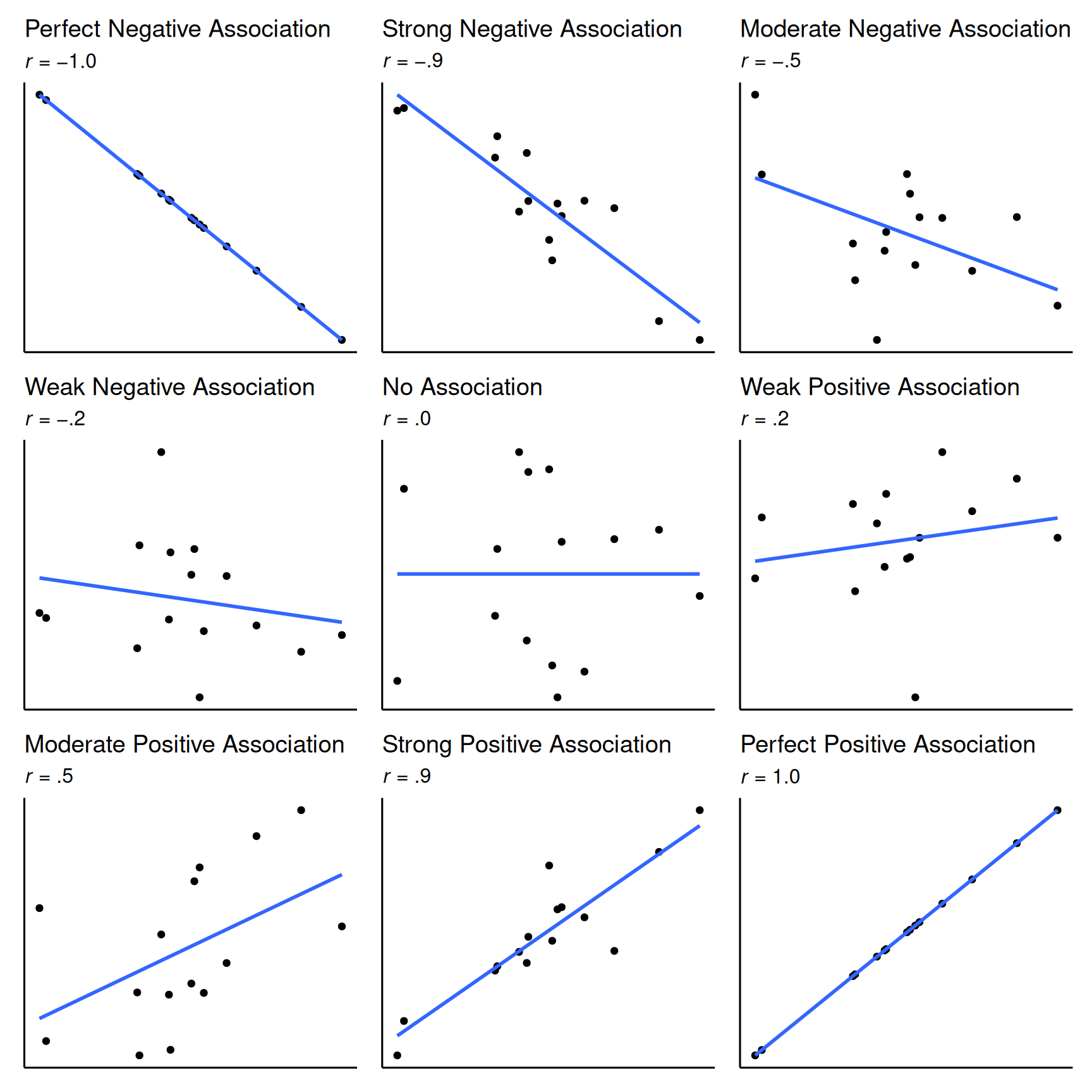
An interactive visualization by Magnusson (2023) on interpreting correlations is at the following link: https://rpsychologist.com/correlation/ (archived at https://perma.cc/G8YR-VCM4)
Keep in mind that the (Pearson) correlation examines the strength of the linear association between two variables. If the association between two variables is nonlinear, the (Pearson) correlation provides the strength of the linear trend and may not provide a meaningful index of the strength of the association between the variables. For instance, Anscombe’s quartet includes four sets of data that have nearly identical basic descriptive statistics (see Tables 10.1 and 10.2), including the same bivariate correlation, yet have very different distributions and whose association takes very different forms (see Figure 10.3).
| x1 | y1 | x2 | y2 | x3 | y3 | x4 | y4 |
|---|---|---|---|---|---|---|---|
| 10 | 8.04 | 10 | 9.14 | 10 | 7.46 | 8 | 6.58 |
| 8 | 6.95 | 8 | 8.14 | 8 | 6.77 | 8 | 5.76 |
| 13 | 7.58 | 13 | 8.74 | 13 | 12.74 | 8 | 7.71 |
| 9 | 8.81 | 9 | 8.77 | 9 | 7.11 | 8 | 8.84 |
| 11 | 8.33 | 11 | 9.26 | 11 | 7.81 | 8 | 8.47 |
| 14 | 9.96 | 14 | 8.10 | 14 | 8.84 | 8 | 7.04 |
| 6 | 7.24 | 6 | 6.13 | 6 | 6.08 | 8 | 5.25 |
| 4 | 4.26 | 4 | 3.10 | 4 | 5.39 | 19 | 12.50 |
| 12 | 10.84 | 12 | 9.13 | 12 | 8.15 | 8 | 5.56 |
| 7 | 4.82 | 7 | 7.26 | 7 | 6.42 | 8 | 7.91 |
| 5 | 5.68 | 5 | 4.74 | 5 | 5.73 | 8 | 6.89 |
| Property | Value |
|---|---|
| Sample size | 11 |
| Mean of X | 9.0 |
| Mean of Y | ~7.5 |
| Variance of X | 11.0 |
| Variance of Y | ~4.1 |
| Equation of regression line | Y = 3 + 0.5X |
| Standard error of slope | 0.118 |
| One-sample t-statistic | 4.24 |
| Sum of squares of X | 110.0 |
| Regression sum of squares | 27.50 |
| Residual sum of squares of Y | 13.75 |
| Correlation coefficient | .816 |
| Coefficient of determination | .67 |
Code
par(mfrow = c(2,2))
plot(
anscombe$x1,
anscombe$y1,
xlab = "x",
ylab = "y",
xlim = c(0,20),
ylim = c(0,15),
main =
substitute(
paste(italic(r), " = ", x, sep = ""),
list(x = round(cor.test(x = anscombe$x1, y = anscombe$y1)$estimate, 2))))
abline(lm(
y1 ~ x1,
data = anscombe),
col = "black",
lty = 2)
plot(
anscombe$x2,
anscombe$y2,
xlab = "x",
ylab = "y",
xlim = c(0,20),
ylim = c(0,15),
main = substitute(
paste(italic(r), " = ", x, sep = ""),
list(x = round(cor.test(x = anscombe$x2, y = anscombe$y2)$estimate, 2))))
abline(lm(
y2 ~ x2,
data = anscombe),
col = "black",
lty = 2)
plot(
anscombe$x3,
anscombe$y3,
xlab = "x",
ylab = "y",
xlim = c(0,20),
ylim = c(0,15),
main = substitute(
paste(italic(r), " = ", x, sep = ""),
list(x = round(cor.test(x = anscombe$x3, y = anscombe$y3)$estimate, 2))))
abline(lm(
y3 ~ x3,
data = anscombe),
col = "black",
lty = 2)
plot(
anscombe$x4,
anscombe$y4,
xlab = "x",
ylab = "y",
xlim = c(0,20),
ylim = c(0,15),
main = substitute(
paste(italic(r), " = ", x, sep = ""),
list(x = round(cor.test(x = anscombe$x4, y = anscombe$y4)$estimate, 2))))
abline(lm(
y4 ~ x4,
data = anscombe),
col = "black",
lty = 2)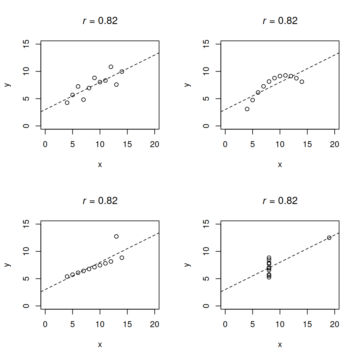
Also note that, although the (Pearson) correlation reflects the strength of the (linear) association between two variables, it does not reflect the (unstandardized) slope of that association, as depicted in Figure 10.4.
) correlation coefficient of $x$ and $y$ for each set. The ([Pearson](#sec-correlationExamplesPearson)) correlation reflects the strength and direction of a linear association (top row), but not the slope of that association (middle), nor many aspects of nonlinear associations (bottom). N.B.: the figure in the center has a slope of 0 but in that case the correlation coefficient is undefined because the variance of $y$ is zero. From <https://en.wikipedia.org/wiki/File:Correlation_examples2.svg>.](images/correlationExamples.png)
The Pearson correlation coefficient can be greatly impacted by the extent of variability in the data, differences in the shapes of the two distributions, nonlinearity, outliers, characteristics of the sample, and measurement error (Goodwin & Leech, 2006). These factors tend to have greater impact when the sample size is smaller (compared to when the sample size is larger). The Pearson correlation coefficient tends to be smaller when:
- there is low variability in one or both variables (i.e., restricted range)
- the two distributions show dissimilar shapes (in terms of skewness and kurtosis)
- the underlying association is nonlinear, such that Pearson correlation does not capture the association
- outliers weaken the apparent linear trend
- the association differs across subgroups of the sample (i.e., moderation)
- the data contain random measurement error
By contrast, the association between two variables can be artificially inflated by factors such as:
- outliers that happen to fall along a linear trend
- systematic measurement error (e.g., common method bias)
- third variable confounding
10.4 Example: Player Height and Fantasy Points
Is there an association between a player’s height and the number of fantasy points they score? We can examine this possibility separately by position.
First, let’s examine descriptive statistics of height and fantasy points (height is measured in inches):
Code
player_stats_seasonal |>
dplyr::select(height, fantasyPoints) |>
dplyr::summarise(across(
everything(),
.fns = list(
n = ~ length(na.omit(.)),
missingness = ~ mean(is.na(.)) * 100,
M = ~ mean(., na.rm = TRUE),
SD = ~ sd(., na.rm = TRUE),
min = ~ min(., na.rm = TRUE),
max = ~ max(., na.rm = TRUE),
q10 = ~ quantile(., .10, na.rm = TRUE), # 10th quantile
q90 = ~ quantile(., .90, na.rm = TRUE), # 90th quantile
range = ~ max(., na.rm = TRUE) - min(., na.rm = TRUE),
IQR = ~ IQR(., na.rm = TRUE),
MAD = ~ mad(., na.rm = TRUE),
CV = ~ sd(., na.rm = TRUE) / mean(., na.rm = TRUE),
median = ~ median(., na.rm = TRUE),
pseudomedian = ~ DescTools::HodgesLehmann(., na.rm = TRUE),
mode = ~ petersenlab::Mode(., multipleModes = "mean"),
skewness = ~ psych::skew(., na.rm = TRUE),
kurtosis = ~ psych::kurtosi(., na.rm = TRUE)),
.names = "{.col}.{.fn}")) |>
tidyr::pivot_longer(
cols = everything(),
names_to = c("variable","index"),
names_sep = "\\.") |>
tidyr::pivot_wider(
names_from = index,
values_from = value)10.4.1 Covariance
The covariance is an unstandardized index of the association between two variables. It represents the average product of two variables’ deviations from their respective means. The formula for (sample) covariance is in Equation 10.1 and is the numerator to the formula for correlation.
\[ \begin{aligned} \text{Cov}(x, y) &= \frac{1}{n - 1} \sum_{i=1}^{n} (x_i - \bar{x})(y_i - \bar{y})\\ &= r_{xy} \cdot s_x \cdot s_y \end{aligned} \tag{10.1}\]
where \(n\) is the sample size, \(x\) is the predictor variable, \(y\) is the outcome variable, \(x_i\) is the ith observation on the predictor variable, \(y_i\) is the ith observation of the outcome variable, \(\bar{x}\) is the mean of the predictor variable, \(\bar{y}\) is the mean of the outcome variable, \(r_{xy}\) is the correlation between the predictor and outcome variables, \(s_x\) is the standard deviation of the predictor variable, and \(s_y\) is the standard deviation of the outcome variable.
For instance, we can calculate the covariance between two variables manually (we subset to just those rows that have data on both \(x\) and \(y\) to ensure we compute the means using the same values that are included in the estimate of the covariance):
Code
complete_cases <- player_stats_seasonal[complete.cases(player_stats_seasonal$height, player_stats_seasonal$fantasyPoints),]
n <- nrow(complete_cases)
x <- complete_cases$height
y <- complete_cases$fantasyPoints
x_mean <- mean(complete_cases$height)
y_mean <- mean(complete_cases$fantasyPoints)
cov_manual <- sum((x - x_mean) * (y - y_mean)) / (n - 1)
cov_manual[1] -11.60278The covariance of a variable with itself is the variable’s variance:
\[ \begin{aligned} \text{Cov}(x, x) &= \frac{1}{n - 1} \sum_{i=1}^{n} (x_i - \bar{x})(x_i - \bar{x})\\ &= \frac{1}{n - 1} \sum_{i=1}^{n} (x_i - \bar{x})^2 \\ &= \frac{\sum (x_i - \bar{x})^2}{n-1}\\ &= s^2 \end{aligned} \tag{10.2}\]
The following syntax shows the variance-covariance matrix of a set of variables, where the covariance of a variable with itself is the variable’s variance. The variances are the values on the diagonal; the covariances are the values on the off-diagonal.
Code
height weight fantasyPoints
height 6.729743 81.50249 -11.60278
weight 81.502487 1998.16192 -419.50147
fantasyPoints -11.602777 -419.50147 3753.20399If you just want the covariance between two variables, you can use the following syntax.
Code
[1] -11.60278Thus, it appears there is a negative covariance between height and fantasy points in the whole population of National Football League (NFL) players.
As shown below, the negative covariance between height and fantasy points holds when examining just Quarterbacks, Running Backs, Wide Receivers, and Tight Ends.
Code
height fantasyPoints
height 7.854615 -6.065242
fantasyPoints -6.065242 7523.304287We can also examine the association separately by position. Here is the association for Quarterbacks:
Code
height fantasyPoints
height 2.861762 9.229307
fantasyPoints 9.229307 12414.569031Here is the association for Running Backs:
Code
height fantasyPoints
height 3.251755 2.183237
fantasyPoints 2.183237 7929.855501Here is the association for Wide Receivers:
Code
height fantasyPoints
height 5.502846 16.13002
fantasyPoints 16.130020 7013.83303Here is the association for Tight Ends:
Code
height fantasyPoints
height 1.872906 3.733876
fantasyPoints 3.733876 3337.287052Interestingly, there is a positive covariance between height and fantasy points when examining each position separately. This is an example of Simpson’s paradox, where the sign of an association differs at different levels of analysis, as described in Section 12.2.2. There is a negative covariance between height and fantasy points when examining Quarterbacks, Running Backs, Wide Receivers, and Tight Ends altogether, but there is a positive covariance between height and fantasy points when examining the association between each position separately. That is, if you were to examine all positions together, you might assume that being taller might be disadvantageous to scoring fantasy fantasy points; however, once we examine the association within a given position, it emerges that height appears to be somewhat advantageous, if anything, for scoring fantasy points.
The covariance is unstandardized—its metric depends on the metrics of the two variables examined in the association. However, it can be helpful to use a standardized index of the association between the variables. A standardized index means that the index is on a common metric and does not depend on the metrics of the two variables. This is valuable because it allows fairly comparing the strength of associations between sets of variables with different metrics, which is meaningful for estimating the effect size—i.e., the strength of the association. The Pearson correlation coefficient, \(r\), is an example of a standardized index of the covariance between two variables because it has a common metric (whose possible values range from −1 to +1, regardless of the variables examined in the association). We can convert a covariance to a correlation by standardizing it; i.e., by dividing by the multiplication of the standard deviation of \(x\) and the standard deviation of \(y\), as in Equation 9.28.
For instance, for the covariance between height and fantasy points, we can convert it to a correlation:
Code
[1] -11.60278[1] -0.07754637[1] -0.07754637We can also convert a correlation back to covariance using the formula in Equation 10.1.
10.4.2 Pearson Correlation
Correlation is a standardized index of the association between two variables. Pearson correlation is the most common type of correlation. The formula for Pearson correlation is in Equation 9.28. Pearson correlation assumes that the variables are interval or ratio level of measurement. If the data are ordinal, Spearman correlation is more appropriate.
The following syntax shows the Pearson correlation matrix of a set of variables.
Code
height weight fantasyPoints
height 1.00000000 0.7030152 -0.07754637
weight 0.70301523 1.0000000 -0.18119019
fantasyPoints -0.07754637 -0.1811902 1.00000000Notice the diagonal values are all 1.0. That is because a variable is perfectly correlated with itself. Also notice that the values above the diagonal are a mirror image of (i.e., they are the same as) the respective values below the diagonal. The association between two variables is the same regardless of the order (i.e., which is the predictor variable and which is the outcome variable); that is, the association between variables A and B is the same as the association between variables B and A.
You can compute a correlation manually using the z scores, as in Equation 9.28:
[1] -0.07754456If you just want the Pearson correlation between two variables, you can use the following syntax.
Pearson's product-moment correlation
data: height and fantasyPoints
t = -16.116, df = 42933, p-value < 2.2e-16
alternative hypothesis: true correlation is not equal to 0
95 percent confidence interval:
-0.08694158 -0.06813736
sample estimates:
cor
-0.07754637 The \(r\) value (-.08) is slightly negative. The effect size of the association is small—for what is considered a small, medium, and large effect size for \(r\) values, see Section 9.4.2.10. The number of degrees of freedom (\(df\)) for a statistical test of a correlation coefficient is in Equation 10.3. The \(p\)-value is less than .05, so it is a statistically significant correlation. We could report this finding as follows: There was a statistically significant, weak negative association between height and fantasy points (\(r(42933) = -.08\), \(p < .001\)); the taller a player was, the fewer fantasy points they tended to score.
\[ df = n - 2 \tag{10.3}\]
Now let’s examine the association separately by position. Here is the association for Quarterbacks:
Pearson's product-moment correlation
data: height and fantasyPoints
t = 2.2417, df = 2091, p-value = 0.02508
alternative hypothesis: true correlation is not equal to 0
95 percent confidence interval:
0.006132083 0.091618750
sample estimates:
cor
0.04896509 Here is the association for Running Backs:
Pearson's product-moment correlation
data: height and fantasyPoints
t = 0.84914, df = 3900, p-value = 0.3959
alternative hypothesis: true correlation is not equal to 0
95 percent confidence interval:
-0.01778991 0.04495503
sample estimates:
cor
0.01359594 Here is the association for Wide Receivers:
Pearson's product-moment correlation
data: height and fantasyPoints
t = 6.1913, df = 5648, p-value = 6.389e-10
alternative hypothesis: true correlation is not equal to 0
95 percent confidence interval:
0.05614807 0.10794872
sample estimates:
cor
0.08210385 Here is the association for Tight Ends:
Pearson's product-moment correlation
data: height and fantasyPoints
t = 2.649, df = 3139, p-value = 0.008113
alternative hypothesis: true correlation is not equal to 0
95 percent confidence interval:
0.01227496 0.08206699
sample estimates:
cor
0.04722861 The sign of the association was positive for each position, suggesting that, for a given position (among Quarterbacks, Running Backs, Wide Receivers, and Tight Ends), taller players tend to score more fantasy points. However, the effect size is small. Moreover, as described in Section 10.8, just because there is an association between variables does not mean that the association reflects a causal effect.
10.4.3 Scatterplot with Best-Fit Line
A scatterplot with best-fit line is in Figure 10.5.
Code
plot_scatterplot <- ggplot2::ggplot(
data = player_stats_seasonal |> filter(position %in% c("QB","RB","WR","TE")),
aes(
x = height,
y = fantasyPoints)) +
geom_point(
aes(
text = player_display_name, # add player name for mouse over tooltip
label = season), # add season for mouse over tooltip
alpha = 0.05) +
geom_smooth(
method = "lm",
color = "black") +
geom_smooth() +
coord_cartesian(
ylim = c(0,NA),
expand = FALSE) +
labs(
x = "Player Height (Inches)",
y = "Fantasy Points (Season)",
title = "Fantasy Points (Season) by Player Height",
subtitle = "(Among QBs, RBs, WRs, and TEs)"
) +
theme_classic()
plotly::ggplotly(plot_scatterplot)Examining the linear line of best fit, we would see that there is a slight negative slope, consistent with a weak negative association. However, the nonlinear best-fit line suggests that there may be an inverted-U-shaped association, which might suggest that there may be an “optimal range of height,” where being too tall or too short may be a disadvantage. We now examine the association between height and fantasy points separately by position in Figure 10.6.
Code
plot_scatterplotByPosition <- ggplot2::ggplot(
data = player_stats_seasonal |> filter(position %in% c("QB","RB","WR","TE")),
aes(
x = height,
y = fantasyPoints,
color = position,
fill = position)) +
geom_point(
aes(
text = player_display_name, # add player name for mouse over tooltip
label = season), # add season for mouse over tooltip
alpha = 0.7) +
geom_smooth(
method = "lm",
color = "black") +
geom_smooth(
method = "loess",
span = 0.5) +
coord_cartesian(
ylim = c(0,NA),
expand = FALSE) +
labs(
x = "Player Height (Inches)",
y = "Fantasy Points (Season)",
title = "Fantasy Points (Season) by Player Height and Position"
) +
guides(fill = "none") +
theme_classic()
plotly::ggplotly(plot_scatterplotByPosition)Examining the association between height and fantasy points separately by position, it appears that there is an inverted-U-shaped associations for Wide Receivers, a relatively flat association for Running Backs and Tight Ends, and a nonlinear association among Quarterbacks. Interestingly, the best-fit lines suggest that the different positions have different height ranges, which is confirmed in Figure 10.7.
Code
ggplot2::ggplot(
data = player_stats_seasonal |>
filter(position %in% c("QB","RB","WR","TE")),
mapping = aes(
x = height,
y = position,
group = position,
fill = position)
) +
ggridges::geom_density_ridges(
bandwidth = 0.6
) +
labs(
x = "Height (inches)",
y = "Position",
title = "Ridgeline Plot of Player Height by Position"
) +
theme_classic() +
theme(
legend.position = "none",
axis.title.y = element_text(angle = 0, vjust = 0.5)) # horizontal y-axis title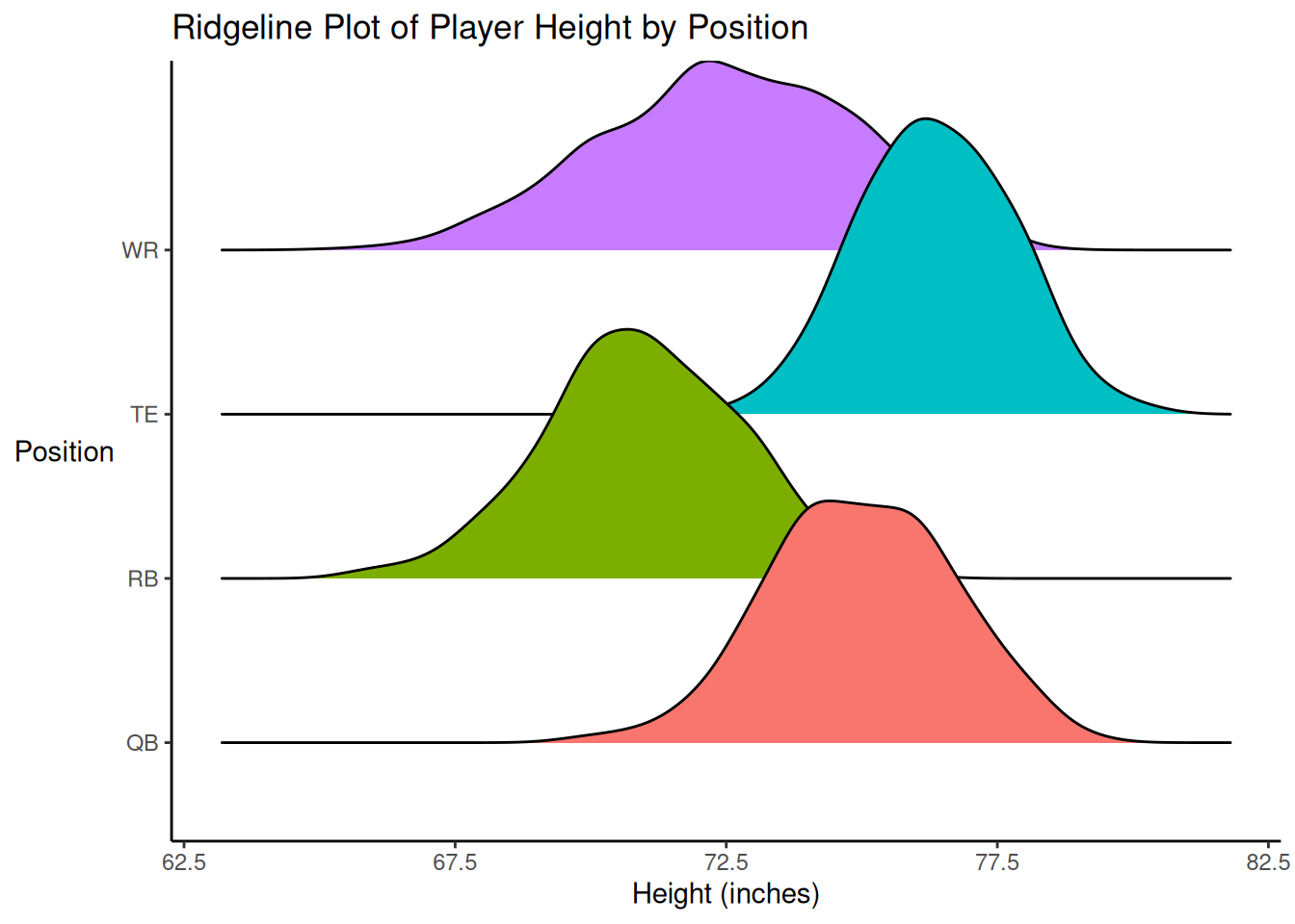
According to the distributions of player height by position (among Quarterbacks, Running Backs, Wide Receivers, and Tight Ends), Running Backs tend to be the shortest, followed by Wide Receivers; Tight Ends tend to be the tallest, followed by Quarterbacks. Wide Receivers showed the greatest variability; some were quite short, whereas others were quite tall.
10.4.4 Rank Correlation: Spearman’s Rho (\(\rho\))
Spearman’s rho (\(\rho\)) is a rank correlation. Spearman’s rho does not assume that the data are interval or ratio level of measurement. Unlike Pearson correlation, Spearman’s rho allows estimating associations among variables that are ordinal level of measurement.
For instance, using Spearman’s rho, we could examine the association between a player’s draft round and their fantasy points, because draft round is an ordinal variable:
Code
draft_round fantasyPoints
draft_round 1.0000000 -0.3504795
fantasyPoints -0.3504795 1.0000000
Spearman's rank correlation rho
data: draft_round and fantasyPoints
S = 6.2694e+12, p-value < 2.2e-16
alternative hypothesis: true rho is not equal to 0
sample estimates:
rho
-0.3504795 Using Spearman’s rho, there is a negative association between draft round and fantasy points (\(r(30311) = -.35\), \(p < .001\)); unsurprisingly, the earlier the round a player is drafted, the more fantasy points they tend to score.
10.4.5 Partial Correlation
A partial correlation examines the association between variables after controlling for one or more variables. Below, we examine a partial Pearson correlation between height and fantasy points after controlling for age using the the psych::partial.r() function from the psych package (Revelle, 2025).
Code
partial correlations
height fantasyPoints
height 1.00 -0.08
fantasyPoints -0.08 1.00Below, we examine a partial Spearman’s rho rank correlation between height and fantasy points after controlling for age.
10.4.6 Nonlinear Correlation
Examples of a nonlinear correlation include the correlation ratio (\(\eta\); Goodwin & Leech, 2006), distance correlation, and the xi (\(\xi\)) coefficient (Chatterjee, 2021). These estimates of nonlinear correlation only range from 0–1 (where 0 represents no association and 1 represents a strong association), so they are interpreted differently than a traditional correlation coefficient (which can be negative).
Here is how to compute the correlation ratio (eta; \(\eta\)) using the stats::aov() and effectsize::eta_squared() functions:
Code
mod <- stats::aov(
fantasyPoints ~ factor(height), # convert the predictor variable to a categorical variable (i.e., factor); if there are too many unique values, can also consider binning the variable into ranges
data = player_stats_seasonal)
etaSquared <- effectsize::eta_squared(mod)
print(etaSquared, digits = 9)# Effect Size for ANOVA
Parameter | Eta2 | 95% CI
---------------------------------------------------------
factor(height) | 0.009078383 | [0.007334819, 1.000000000]
- One-sided CIs: upper bound fixed at [1.000000000].Code
correlationRatio <- etaSquared
cols_to_sqrt <- intersect(
colnames(correlationRatio),
c("Eta2", "CI_low", "CI_high"))
correlationRatio[cols_to_sqrt] <- sqrt(correlationRatio[cols_to_sqrt]) # take the square root of eta-squared to get eta
correlationRatio <- correlationRatio |>
rename(Eta = Eta2)
print(correlationRatio, digits = 9)# Effect Size for ANOVA
Parameter | Eta | 95% CI
---------------------------------------------------------
factor(height) | 0.095280550 | [0.085643557, 1.000000000]
- One-sided CIs: upper bound fixed at [1.000000000].Code
[1] 0.009078383[1] 0.09528055We can estimate a distance correlation using the correlation::correlation() function of the correlation package (Makowski et al., 2020, 2025).
Code
A nonlinear correlation can be estimated using the xi (\(\xi\)) coefficient from the XICOR::xicor() function of the XICOR package (Chatterjee, 2021; Holmes & Chatterjee, 2023):
10.4.7 Correlation Matrix
The petersenlab package (Petersen, 2025a) contains the petersenlab::cor.table() function that generates a correlation matrix of variables, including the \(r\) value, number of observations (\(n\)), asterisks denoting statistical significance, and \(p\)-value for each association. The asterisks follow the following traditional convention for statistical significance: \(^\dagger p < .1\); \(^* p < .05\); \(^{**} p < .01\); \(^{***} p < .001\). Here is a Pearson correlation matrix:
Here is a Spearman correlation matrix:
Code
Here is a correlation matrix of variables that includes just the \(r\) value and asterisks denoting the statistical significance of the association, for greater concision.
Code
Here is a correlation matrix of variables that includes just the \(r\) value for even greater concision.
Code
The petersenlab package (Petersen, 2025a) contains the petersenlab::partialcor.table() function that generates a partial correlation matrix. Here is a partial correlation matrix, controlling for the player’s age:
10.4.8 Correlogram
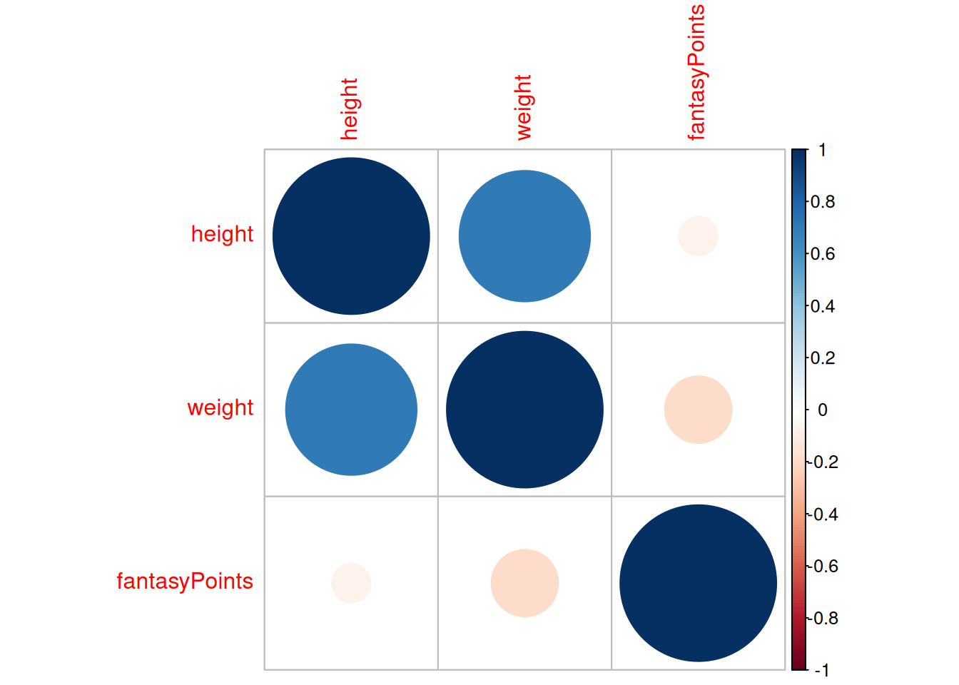
We can depict a correlation matrix plot (correlogram) using the GGally::ggcorr() function of the GGally (Schloerke et al., 2025) package, as shown in Figure 10.8.
10.5 Addressing Non-Independence of Observations
Please note that the \(p\)-value for a correlation assumes that the observations are independent—in particular, that the residuals are not correlated. However, the observations are not independent in the player_stats_seasonal dataframe used above, because the same player has multiple rows—one row corresponding to each season they played. This non-independence violates the traditional assumptions of the significance test of a correlation. We could address this assumption by analyzing only one season from each player or by estimating the significance of the correlation coefficient using cluster-robust standard errors. For simplicity, we present results above from the whole dataframe. In Chapter 12, we discuss mixed model approaches that handle repeated measures and other data that violate assumptions of non-independence that are shared by correlation and multiple regression; assumptions of multiple regression are described in Section 11.5. In Section 11.14, we demonstrate how to account for non-independence of observations using cluster-robust standard errors.
10.6 Impact of Outliers
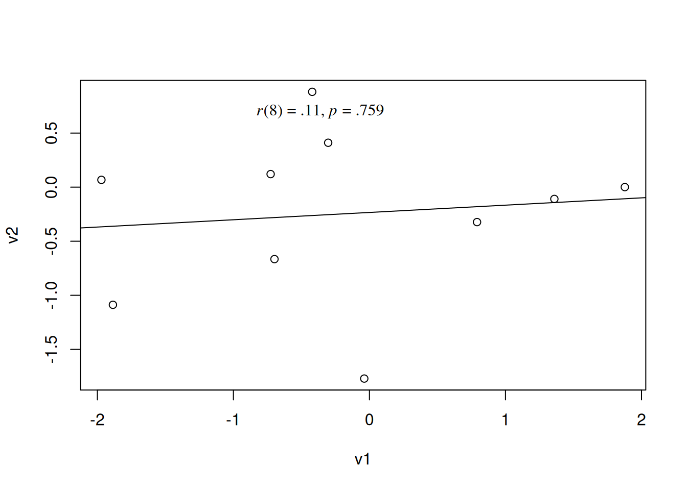
The correlation coefficient is strongly impacted by outliers—i.e., extreme (i.e., very large or very small) values relative to the other observations. Outliers can arise from errors that arise from data collection, measurement, or data entry, or they could represent valid (albeit atypical) values (Goodwin & Leech, 2006). Outliers can either artificially weaken the estimate of association—if they weaken the apparent linear trend—or artificially strengthen it—if they happen to fall along a linear trend. Consider the following example:
Pearson's product-moment correlation
data: v1 and v2
t = 0.31786, df = 8, p-value = 0.7587
alternative hypothesis: true correlation is not equal to 0
95 percent confidence interval:
-0.5571223 0.6926038
sample estimates:
cor
0.1116785 The associated scatterplot and best-fit line is in Figure 10.9.
Now, let’s add one outlier.
Pearson's product-moment correlation
data: v1 and v2
t = 2.7132, df = 9, p-value = 0.02387
alternative hypothesis: true correlation is not equal to 0
95 percent confidence interval:
0.1186112 0.9060613
sample estimates:
cor
0.6707604 The associated scatterplot and best-fit line for the updated data are in Figure 10.10.
Code
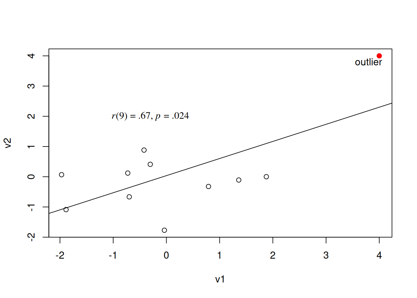
Note how the association was not close to being statistically significant without the outlier, but with the outlier added, the association is statistically significant. One way to combat this is to use methods for estimating the association between variables that are robust to (i.e., less impacted by) outliers. In the next section, we describe robust correlation methods.
10.6.1 Examining Robust Correlation
There are various approaches to estimating correlation in the presence of outliers—so-called robust correlation methods.
One approach is the biweight midcorrelation, which is based on the median rather than the mean, and is thus less sensitive to outliers. Another approach is the percentage bend correlation, which gives less weight to observations that are farther away from the median. We can estimate the each using the correlation::correlation() function of the correlation package (Makowski et al., 2020, 2025).
10.7 Impact of Restricted Range
In addition to being impacted by outliers, correlations can also be greatly impacted by restricted variability or restricted range (Petersen, 2024, 2025b). Correlation depends on variability; if there is no or limited variability, it can be difficult to detect an association with another variable. Thus, if a variable has restricted range—such as owing to a floor effect or ceiling effect—that tends to artificially weaken associations. For instance, a floor effect is one in which many of the scores are the lowest possible score. By contrast, a ceiling effect is one in which many of the scores are the highest possible score.
Consider the following association between passing attempts and expected points added (EPA) via passing. Expected points added from a given play is calculated as the difference between a team’s expected points before the play and the team’s expected points after the play. This can be summed across all passing plays to determine a player’s EPA from passing during a given season.
Pearson's product-moment correlation
data: player_stats_seasonal$attempts and player_stats_seasonal$passing_epa
t = 25.344, df = 2858, p-value < 2.2e-16
alternative hypothesis: true correlation is not equal to 0
95 percent confidence interval:
0.3979683 0.4578357
sample estimates:
cor
0.428372 There is a statistically significant, moderate positive association between passing attempts and expected points added (EPA) via passing, as depicted in Figure 10.11.
Code
plot_scatterplotWithoutRangeRestriction <- ggplot2::ggplot(
data = player_stats_seasonal,
aes(
x = attempts,
y = passing_epa)) +
geom_point(
aes(
text = player_display_name, # add player name for mouse over tooltip
label = season), # add season for mouse over tooltip
alpha = 0.3) +
geom_smooth(
method = "lm") +
#geom_smooth() +
coord_cartesian(
expand = FALSE) +
labs(
x = "Player's Passing Attempts",
y = "Player's Expected Points Added (EPA) via Passing",
title = "Player's Passing Expected Points Added (EPA)\nby Passing Attempts (Season)",
#subtitle = ""
) +
theme_classic()
plotly::ggplotly(plot_scatterplotWithoutRangeRestriction)Now, consider the same association when we restrict the range to examine only those players who had fewer than 450 pass attempts in a season (thus resulting in less variability):
Code
Pearson's product-moment correlation
data: pull(select(filter(player_stats_seasonal, attempts < 450), attempts)) and pull(select(filter(player_stats_seasonal, attempts < 450), passing_epa))
t = -1.9985, df = 2386, p-value = 0.04577
alternative hypothesis: true correlation is not equal to 0
95 percent confidence interval:
-0.0808589203 -0.0007694173
sample estimates:
cor
-0.04087983 The association is no longer positive and is weak in terms of effect size, as depicted in Figure 10.12.
Code
plot_scatterplotWithRangeRestriction <- ggplot2::ggplot(
data = player_stats_seasonal |> filter(attempts < 450),
aes(
x = attempts,
y = passing_epa)) +
geom_point(
aes(
text = player_display_name, # add player name for mouse over tooltip
label = season), # add season for mouse over tooltip
alpha = 0.3) +
geom_smooth(
method = "lm") +
#geom_smooth() +
coord_cartesian(
expand = FALSE) +
labs(
x = "Player's Passing Attempts",
y = "Player's Expected Points Added (EPA) via Passing",
title = "Player's Passing Expected Points Added (EPA)\nby Passing Attempts (Season)",
subtitle = "(Among Players with < 450 Passing Attempts)"
) +
theme_classic()
plotly::ggplotly(plot_scatterplotWithRangeRestriction)10.8 Correlation Does Not Imply Causation
As described in Section 8.5.2.1, correlation does not imply causation. There are several reasons (described in Section 8.5.2.1) that, just because X is correlated with Y does not necessarily mean that X causes Y. However, correlation can still be useful. In order for two processes to be causally related, they must be associated, as described in Section 13.4. That is, association is necessary but insufficient for causality.
10.9 Conclusion
Correlation is a standardized index of the association between variables. The correlation coefficient (\(r\)) ranges from −1 to +1, and indicates the sign and magnitude of the association. Although correlation does not imply causation, identifying associations between variables can still be useful because association is a necessary (but insufficient) condition for causality. The correlation coefficient can be heavily impacted by outliers and restricted range.
10.10 Session Info
R version 4.6.1 (2026-06-24)
Platform: x86_64-pc-linux-gnu
Running under: Ubuntu 24.04.4 LTS
Matrix products: default
BLAS: /usr/lib/x86_64-linux-gnu/openblas-pthread/libblas.so.3
LAPACK: /usr/lib/x86_64-linux-gnu/openblas-pthread/libopenblasp-r0.3.26.so; LAPACK version 3.12.0
locale:
[1] LC_CTYPE=C.UTF-8 LC_NUMERIC=C LC_TIME=C.UTF-8
[4] LC_COLLATE=C.UTF-8 LC_MONETARY=C.UTF-8 LC_MESSAGES=C.UTF-8
[7] LC_PAPER=C.UTF-8 LC_NAME=C LC_ADDRESS=C
[10] LC_TELEPHONE=C LC_MEASUREMENT=C.UTF-8 LC_IDENTIFICATION=C
time zone: UTC
tzcode source: system (glibc)
attached base packages:
[1] stats graphics grDevices utils datasets methods base
other attached packages:
[1] patchwork_1.3.2 lubridate_1.9.5 forcats_1.0.1 stringr_1.6.0
[5] dplyr_1.2.1 purrr_1.2.2 readr_2.2.0 tidyr_1.3.2
[9] tibble_3.3.1 tidyverse_2.0.0 ggridges_0.5.7 GGally_2.4.0
[13] ggplot2_4.0.3 effectsize_1.0.3 correlation_0.8.8 DescTools_0.99.60
[17] psych_2.6.5 XICOR_0.4.1 petersenlab_1.2.3
loaded via a namespace (and not attached):
[1] Rdpack_2.6.6 DBI_1.3.0 mnormt_2.1.2
[4] gridExtra_2.3.1 gld_2.6.8 sandwich_3.1-2
[7] readxl_1.5.0 rlang_1.3.0 magrittr_2.0.5
[10] multcomp_1.4-31 otel_0.2.0 e1071_1.7-17
[13] compiler_4.6.1 mgcv_1.9-4 vctrs_0.7.3
[16] reshape2_1.4.5 quadprog_1.5-8 pkgconfig_2.0.3
[19] fastmap_1.2.0 backports_1.5.1 labeling_0.4.3
[22] pbivnorm_0.6.0 rmarkdown_2.31 psychTools_2.6.4
[25] tzdb_0.5.0 haven_2.5.5 nloptr_2.2.1
[28] xfun_0.60 jsonlite_2.0.0 parallel_4.6.1
[31] lavaan_0.7-2 cluster_2.1.8.2 R6_2.6.1
[34] stringi_1.8.7 RColorBrewer_1.1-3 boot_1.3-32
[37] rpart_4.1.27 estimability_2.0.0 cellranger_1.1.0
[40] Rcpp_1.1.2 knitr_1.51 zoo_1.8-15
[43] parameters_0.29.2 base64enc_0.1-6 timechange_0.4.0
[46] Matrix_1.7-5 splines_4.6.1 nnet_7.3-20
[49] tidyselect_1.2.1 rstudioapi_0.19.0 yaml_2.3.12
[52] codetools_0.2-20 lattice_0.22-9 plyr_1.8.9
[55] withr_3.0.3 bayestestR_0.18.1 S7_0.2.2
[58] coda_0.19-4.1 evaluate_1.0.5 foreign_0.8-91
[61] survival_3.8-6 ggstats_0.13.0 proxy_0.4-29
[64] pillar_1.11.1 checkmate_2.3.4 stats4_4.6.1
[67] reformulas_0.4.4 insight_1.5.2 plotly_4.12.1
[70] generics_0.1.4 mix_1.0-13 hms_1.1.4
[73] scales_1.4.0 rootSolve_1.8.2.4 minqa_1.2.8
[76] xtable_1.8-8 class_7.3-23 glue_1.8.1
[79] emmeans_2.0.4 Hmisc_5.2-6 lmom_3.3
[82] tools_4.6.1 data.table_1.18.4 lme4_2.0-6
[85] Exact_3.3 fs_2.1.0 mvtnorm_1.4-2
[88] grid_4.6.1 mitools_2.4 crosstalk_1.2.2
[91] rbibutils_2.4.1 datawizard_1.3.1 colorspace_2.1-3
[94] nlme_3.1-169 htmlTable_2.5.0 Formula_1.2-5
[97] cli_3.6.6 expm_1.0-0 viridisLite_0.4.3
[100] gtable_0.3.6 digest_0.6.39 TH.data_1.1-5
[103] htmlwidgets_1.6.4 farver_2.1.2 htmltools_0.5.9
[106] lifecycle_1.0.5 httr_1.4.8 MASS_7.3-65