I want your feedback to make the book better for you and other readers. If you find typos, errors, or places where the text may be improved, please let me know. The best ways to provide feedback are by GitHub or hypothes.is annotations.
You can leave a comment at the bottom of the page/chapter, or open an issue or submit a pull request on GitHub: https://github.com/isaactpetersen/Fantasy-Football-Analytics-Textbook
Alternatively, you can leave an annotation using hypothes.is.
To add an annotation, select some text and then click the
symbol on the pop-up menu.
To see the annotations of others, click the
symbol in the upper right-hand corner of the page.
27 Sports and Cognitive Psychology
This chapter provides an overview of some of the roles of cognitive psychology and analytics in sports.
27.1 Getting Started
27.1.1 Load Packages
27.1.2 Download Football Data
27.2 Overview
There are a number of ways in which analytics have changed sports (Underwood, 2019; archived at https://perma.cc/PQ5R-TWFA). Here is a summary of some of the key ways that analytics has led to changes.
Much of the history of analytics in sports traces back to Bill James. James was a member of the Society for American Baseball Research (SABR). He published a series of Baseball Abstracts, which included players’ statistics. James published the first Baseball Abstract in 1977 (https://www.pbs.org/thinktank/transcript1197.html; archived at https://perma.cc/Y7J7-GB9V). He coined the term Sabermetrics (which was originally named SABRmetrics, based on the name of the society) to refer to advanced metrics and statistical/empirical analysis of baseball. James believed that traditional statistics like batting average, runs batted in (RBIs), and pitchers’ wins did not reflect a player’s true value—i.e., their contribution to the team’s success. Instead, he advocated for the use of more advanced metrics that could provide a deeper understanding of a player’s performance and value such as on-base percentage (OBP), slugging percentage (SLG), wins above replacement (WAR), and fielding independent pitching (FIP). He also developed advanced metrics such as runs created (RC) and defense efficiency rating (DER).
James’ ideas were slow to catch on among those in baseball. Nevertheless, some people eventually caught on to his ideas—and to good success. Billy Beane, a general manager, used Sabermetrics to help the Oakland Athletics, a small market team with a limited budget, better compete with teams with larger budgets. He used statistics such as on-base percentage to identify player value more accurately, especially for identifying undervalued players. The story was described in Michael Lewis’ book, Moneyball, which was turned into a movie. Following publication of Moneyball, Theo Epstein, who was president of the Boston Red Sox and then of the Chicago Cubs, used sabermetrics to help each win the World Series.
In addition to teams using Sabermetrics to evaluate player talent, teams also began to frequently use statistical analysis to inform decision making during games, which led to key changes in the style of play. For instance, defensive shifts—where defensive players moved to locations on the field where particular hitters were most likely to hit the ball—became more common, attempts to steal bases became less common, there were fewer bunts, batters took more pitches (i.e., watched more pitches without swinging), there were more frequent pitching changes (for particular pitcher–batter matchups; such as to have a right-handed pitcher face a left-handed batter or vice versa), and a greater focus on velocity and spin rate among pitchers. Some of these analytics-driven changes in play style eventually led Major League Baseball (MLB) to make rule changes in an attempt to make the game more exciting to watch, including banning defensive shifts, reducing the number of pitching changes allowed, and making the bases larger and easier to steal.
Although baseball was one of the first major sports to embrace analytics, other sports have been transformed by analytics, as well. For instance, in basketball, there has been a greater focus on three points and buckets close to the rim (e.g., dunks and layups), with way fewer midrange shots (Partnow, 2021). Moreover, star players rest more games (“load management”). Here is an article on how Shane Battier, who was not the quickest, fastest, or most athletic player, used analytics successfully to guard players who were quicker or more athletic than him: https://www.nytimes.com/2009/02/15/magazine/15Battier-t.html (Lewis, 2009; archived at https://web.archive.org/web/20250219225627/https://www.nytimes.com/2009/02/15/magazine/15Battier-t.html).
Football has also seen greater use of analytics, although its uptake has been somewhat slower than in many other sports (Carroll et al., 2023). When asked about how he makes the decision about whether to go for a two-point conversion after a touchdown, Steelers Head Coach Mike Tomlin stated:
“We work a menu of plays in that area over the course of the week. We rank them at the latter part of the week, and then we get into the stadium and we play it by ear. A lot of it has to do with the feel or the flow of the game—maybe what personnel group we think they’re going to match our personnel group with. As we start to play and work the ball down the field on the drives that produce the touchdowns before the point after, we have a little inclination of what their personality might be at least in terms of matching our personnel. All of those things weigh into the decision. It legitimately is a feel thing. I think that’s why you play the game. You can take analytics to baseball and things like that, but football is always going to be football. I got a lot of respect for analytics and numbers, but I’m not going to make judgments based on those numbers. The game is the game. It’s an emotional one played by emotional and driven men. That’s an element of the game you can’t measure. Oftentimes, decisions such as that weigh heavily into the equation.”
— Steelers Head Coach Mike Tomlin, 2015 (archived at https://perma.cc/7CHJ-BTWX)
That is, Mike Tomlin, suggested that he does not take into account analytics when making decisions. Perhaps that is why the Pittsburgh Steelers were voted one of the least analytically advanced teams in the NFL in 2020 (Walder, 2020; archived at https://perma.cc/R7FA-HGGB). Nevertheless, the Steelers did eventually hire a person focused on analytics (Fowler, 2015; archived at https://perma.cc/W7VE-JZQX).
A player talent evaluator for the NFL noted that many people around the league believe that the use of analytics is better suited for baseball than football because baseball involves more games, players, and one-on-one matchups (Reed, 2016; archived at https://web.archive.org/web/20200803205803/https://www.cleveland.com/browns/2016/01/in_an_nfl_divided_over_analyti.html). By contrast, player performance in football may be more dependent on teammates and play calls. The player talent evaluator noted, “In football they don’t know how to use all the numbers yet…They have the data, they have all these different stats but the people I have talked to aren’t completely sure how to use it.” (Reed, 2016; archived at https://web.archive.org/web/20200803205803/https://www.cleveland.com/browns/2016/01/in_an_nfl_divided_over_analyti.html). Some dismiss analytics entirely.
As an example of people dismissing analytics, Figure 27.1 is a 2015 video clip of a football commentator, Mike Patrick, making fun of people who compile statistics for informing decision-making in football, calling the people who compile the numbers “guys who wear socks with flip-flops” (ABC, 2015a). His characterization suggests he believes that people who compile analytics to make recommendations in football are out of touch with the realities of football and do not have the same on-the-field understanding as the coaches and players. The full game is available to watch here (ABC, 2015b).
Nevertheless, more and more people around the league use analytics—likely because it works; for examples of articles, see here (Clark, 2018; archived at https://perma.cc/7BKP-A4GJ) and here (Awbrey, 2020; archived at https://perma.cc/WXE3-53E6). Head Coach Doug Peterson heavily relied on analytics with the Philadelphia Eagles to help them win the 2017 Super Bowl; for more information, see here (Fox, 2021; archived at https://perma.cc/49KQ-R785) and here (Rosenthal, 2018; archived at https://perma.cc/2GRF-8Z5K). Moreover, teams are now using artificial intelligence (AI) to help them prepare for games, evaluate players, make draft selections, and perform game management (Levi, 2025; archived at https://perma.cc/XF2Z-ZZZT).
Examples of changes in football due to the use of analytics include more often going for it on fourth down, a greater emphasis on the passing game, drafting Running Backs later in the draft (and, more generally, valuing Running Backs less), and trading down in the draft to obtain more low picks (rather than having fewer high picks) because top picks are frequently overvalued (Massey & Thaler, 2013). Although both performance and compensation decline with draft order in the NFL, compensation declines more steeply than performance (Massey & Thaler, 2013). The highest value picks—in terms of the greatest expected performance relative to compensation (i.e., performance per dollar)—are near the beginning of the second round of the NFL draft (Massey & Thaler, 2013). According to their analysis, Massey & Thaler (2013) found that the least valuable pick in the first round of the NFL draft (based on expected performance relative to compensation) is the 1st overall pick! Thus, they refer to the first pick as the “loser’s curse” (Massey & Thaler, 2013). In general, the overvaluation of picks tends to be greatest at the top of the draft, even accounting for the possibility of drafting superstars (Massey & Thaler, 2013).
27.3 Coaching and Loss/Risk Aversion
27.3.1 Going for It on Fourth Down
It had been known for a long time that going for it on fourth down would frequently increase a team’s chances of winning. Despite that, historically, teams rarely went for it on fourth down and elected to punt or kick a field goal instead. It is curious that there was such a discrepancy between the decisions that would maximize teams’ winning percentage and the decisions coaches actually made. In many fourth down situations, by punting the ball, coaches actively and systematically made decisions that reduced their team’s chances of winning. One potential explanation for the discrepancy is because of coaches’ risk aversion. As noted in Section 14.4.10, when it is possible to experience either a gain or a loss from a decision, loss aversion bias tends to lead people to make risk-averse decisions (Kahneman, 2011). According to this idea, in the case of failing to successfully convert on fourth down, coaches do not want to have to defend their decision to go for it to the media or the owner or general manager. That is, they may often play not to lose, rather than to win, in order to keep their job. However, in many cases, this is the wrong choice (Moskowitz & Wertheim, 2011).
Rates of going for it on fourth down in the NFL were low until 2017. After the 2017 season, rates of going for it on fourth down increased dramatically, as depicted in Figure 27.2.
Code
nfl_pbp4thDown <- nfl_pbp |>
  filter(down == 4) |>
  filter(!(play_type %in% c("no_play","qb_kneel")))

nfl_pbp4thDown$goForIt <- NA
nfl_pbp4thDown$goForIt[which(nfl_pbp4thDown$play_type %in% c("field_goal","punt"))] <- 0
nfl_pbp4thDown$goForIt[which(nfl_pbp4thDown$play_type %in% c("pass","run"))] <- 1

nfl_pbp4thDownPlotData <- nfl_pbp4thDown |>
  filter(!is.na(goForIt)) |>
  group_by(season) |>
  summarise(
    goForItPct = mean(goForIt, na.rm = TRUE),
    n = n(),
    sd = sd(goForIt),
    se = sd / n
  )

ggplot2::ggplot(
  data = nfl_pbp4thDownPlotData,
  ggplot2::aes(
    x = season,
    y = goForItPct)) +
  geom_point() +
  geom_line() +
  geom_ribbon(
    aes(
      y = goForItPct,
      ymin = goForItPct - qnorm(0.975)*se,
      ymax = goForItPct + qnorm(0.975)*se),
    alpha = 0.2) +
  scale_y_continuous(
    limits = c(0, NA)
  ) +
  scale_x_continuous(
    minor_breaks = seq(0, 3000, 1),
    breaks = seq(0, 3000, 5)
  ) +
  labs(
    x = "Season",
    y = "Proportion of 4th Down Plays that\nare Attempts (to Get the First Down)",
    title = "4th Down Attempts (Proportion) by Season",
  ) +
  theme(axis.title.y = element_text(angle = 0, vjust = 0.5)) + # horizontal y-axis title
  annotate(
    "segment",
    x = 2015,
    xend = 2017,
    y = 0.08,
    yend = 0.123,
    color = "blue",
    linewidth = 1.5,
    alpha = 0.6,
    arrow = arrow()) +
  annotate(
    "text",
    x = 2015,
    y = 0.07,
    label = "Rapid increases in 4th down\nattempts after the 2017 season",
    hjust = 0.5) # center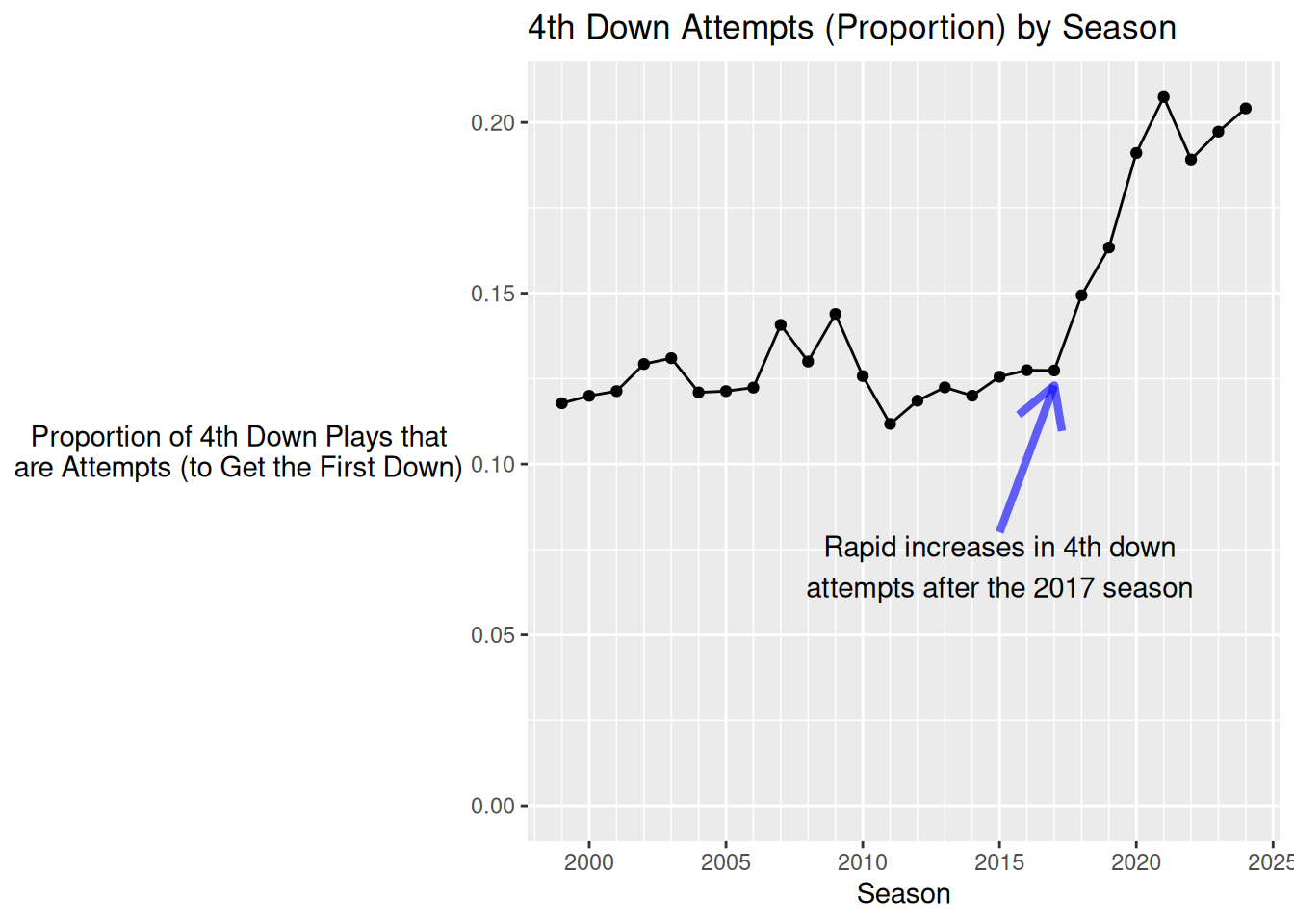
As depicted in the Figure 27.3 [which was adapted from a figure by Ben Baldwin; Baldwin (2023); archived at https://perma.cc/S5D8-3NCU], teams went for it on fourth down nearly twice as often in 2021 compared to 2017, when their win probability was at least 20% (given the current situation at the start of the given play) and they would increase their win probability by going for it. We use the ggtext package (Wilke & Wiernik, 2022) to annotate text:
Code
# labels on the plot
text_df <- tibble(
  label = c(
    "NFL coaches<br>in <span style='color:#00BFC4'>**2021**</span>",
    "NFL coaches<br>in <span style='color:#F8766D'>**2017**</span>"),
  x = c(5, 7),
  y = c(87.5, 22.5),
  angle = c(10, 10),
  color = c("black", "black")
)

nfl_4thdown |>
  filter(
    vegas_wp > .2,
    between(go_boost, -10, 10),
    season %in% c(2017, 2021)) |>
  ggplot(
    aes(
      x = go_boost,
      y = go,
      color = as.factor(season))) +
  geom_vline(xintercept = 0) +
  stat_smooth(
    method = "gam",
    method.args = list(gamma = 1),
    formula = y ~ s(x, bs = "cs", k = 10),
    show.legend = FALSE,
    se = FALSE,
    linewidth = 4) +
  # this is just to get the plot to draw the full 0 to 100 range
  geom_hline(
    yintercept = 100,
    alpha = 0) +
  geom_hline(
    yintercept = 0,
    alpha = 0) +
  ggtext::geom_richtext(
    data = text_df,
    aes(
      x,
      y,
      label = label,
      angle = angle),
    color = "black",
    fill = NA,
    label.color = NA,
    size = 5) +
  theme_classic() +
  labs(
    x = "Gain in win probability by going for it",
    y = "Go-for-it percentage",
    subtitle = "4th down decisions in 2021 versus 2017, win prob. > 20%",
    title = glue::glue("How <span style='color:red'>math</span> is changing football")) +
  theme(
    legend.position = "none",
    plot.title = element_markdown(
      size = 22,
      hjust = 0.5),
    plot.subtitle = element_markdown(
      size = 13.5,
      hjust = 0.5),
    axis.title.x = element_text(
      size = 14,
      face = "bold"),
    axis.title.y = element_text(
      size = 14,
      face = "bold",
      angle = 0, # horizontal y-axis title
      vjust = 0.5)
  ) +
  scale_y_continuous(
    breaks = scales::pretty_breaks(n = 4),
    limits = c(0, 100),
    expand = c(0, 0)) +
  scale_x_continuous(
    breaks = scales::pretty_breaks(n = 10),
    limits = c(-10, 10),
    expand = c(0, 0)) +
  annotate(
    "text",
    x = -1.5,
    y = 70,
    label = "Should\nkick",
    color = "black",
    size = 5) +
  annotate(
    "text",
    x = 1.75,
    y = 70,
    label = "Should\ngo for it",
    color = "black",
    size = 5) +
  annotate(
    "segment",
    x = -.1,
    y = 80,
    xend = -2,
    yend = 80,
    arrow = arrow(length = unit(0.05, "npc")),
    color = "black",
    linewidth = 2) +
  annotate(
    "segment",
    x = .1,
    y = 80,
    xend = 2,
    yend = 80,
    arrow = arrow(length = unit(0.05, "npc")),
    color = "black",
    linewidth = 2)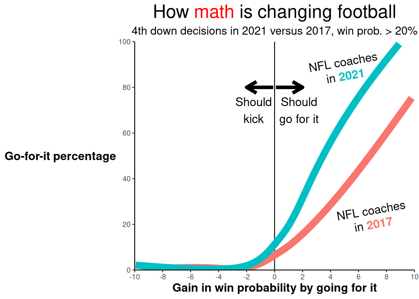
NFL teams were later to implement analytics into their decision making than even teams at lower levels of the sport. Some high school teams, such as the Pulaski Academy Bruins (Little Rock, AR), coached by Kevin Kelley, consistently went for it on fourth down well before 2017 (Moskowitz & Wertheim, 2011).
[Bruins Head Football Coach Kevin] Kelley believes that the “quant jocks” don’t go far enough to validate the no-punting worldview and, more generally, the virtues of risk-taking. “The math guys, the astrophysicist guys, they just do the raw numbers and they don’t figure emotion into it—and that’s the biggest thing of all,” he says. “The built-in emotion involved in football is unbelievable, and that’s where the benefits really pay off.” What he means is this: A defense that stops an opponent on third down is usually ecstatic. They’ve done their job. The punting unit comes on, and the offense takes over. When that defense instead gives up a fourth-down conversion, it has a hugely deflating effect. At Pulaski’s games, you can see the shoulders of the opposing defensive players slump and their eyes look down when they fail to stop the Bruins on fourth down.
Based on Romer’s (2006) analysis of third down plays (because few teams went for it on fourth down), focusing on plays in the first quarter (to remove desperation plays), he identified several general conclusions about fourth-down situations:
- Inside the opponent’s 45-yard line, a team is better off going for it than punting with 6 (or less) yards to go (for a first down).
- Inside the opponent’s 33-yard line, a team is better off going for it with 10 (or less) yards to go (unless little time remains and a field goal would decide the game).
- Once reaching the opponent’s 5-yard line, a team is better off going for it.
- Regardless of field position, a team is always better off going for it with 3 (or less) yards to go.
Nevertheless, out of the fourth down plays Romer (2006) identified between 1998–2000 in which it would have been advantageous to go for it, the team made the suboptimal decision (punting or kicking) 90% of the time. “Inasmuch as an academic paper can become a cult hit, Romer’s made the rounds in NFL executive offices, but most NFL coaches seemed to dismiss his findings as the handiwork of an egghead, polluting art with science.” (Moskowitz & Wertheim, 2011, p. 39).
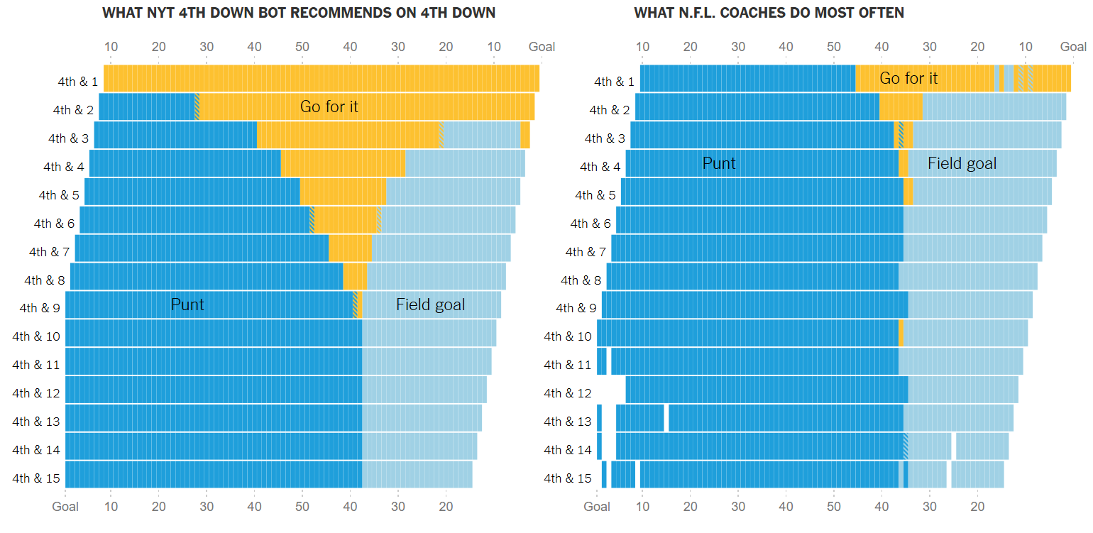
Here is an analysis by the New York Times on when to go for it on fourth down: https://www.nytimes.com/2014/09/05/upshot/4th-down-when-to-go-for-it-and-why.html (NYT 4th Down Bot, 2014; archived at https://perma.cc/KA9Y-BRUD). Here is a fourth down calculator: https://rbsdm.com/stats/fourth_calculator/.
In addition to punting on fourth down, loss aversion bias may lead coaches to make more conservative play-calling, in general, such as running the ball when passing would tend to be more advantageous.
27.4 Challenging a Call
A coach can challenge a call (and have it reviewed) by throwing a red flag onto the field. If, after the review, the play is reversed, the team does not lose a timeout; however, if the play stands as originally called, the team loses a timeout. One task is for coaches to determine when it is optimal to challenge a call. NFL.com provides an opportunity for you to determine whether you should challenge a call: https://operations.nfl.com/learn-the-game/making-the-call/you-make-the-call/.
Tanney (2021) provides a framework for determining whether a coach should challenge a call, based on the expected value of the change in winning probability of a reversal versus a non-reversal:
\[ \begin{aligned} \text{expected value} = \; &\text{Sum}(\text{Probabilities} \times \text{Payouts}) \\ = \; &(\text{Reversal \%})(\text{Positive change in Winning Probability of a Reversal}) + \\ &(1 - \text{Reversal \%})(\text{Negative change in Winning Probability of Losing a Timeout}) \end{aligned} \tag{27.1}\]
27.5 Other Beliefs in Sports
27.5.1 Icing the Kicker
In a 2008 game between the Jets and Raiders, Jets Kicker Jay Feely missed a game-tying field goal to send the game to overtime. However, moments before the snap, the Raiders called a timeout in an attempt to “ice the kicker.” The idea behind icing the kicker is making the kicker think about the pressure of upcoming kick so he gets “cold feet” (metaphorically speaking) and misses the kick. After the brief timeout, Feely got a second chance and made the field goal to send the game into overtime.
After the game, Feely noted, “I heard the whistle before I started, which is an advantage to the kicker…If you’re going to do that, do that before he kicks. I can kick it down the middle, see what the wind does and adjust. It helps the kicker tremendously.” (The Associated Press, 2008; archived at https://perma.cc/U7SV-UE2E).
However, does icing the kicker work? There is mixed evidence on icing the kicker. Some studies find some evidence for lower percentage of iced kicks made compared to non-iced kicks (Goldschmied et al., 2025), whereas other studies do not (e.g., Berry & Wood, 2004; Gonzalez Sanchez et al., 2024; Moskowitz & Wertheim, 2011). This suggests that, if there is such an effect, the effect size is likely very small, and it may better suit the team to use your timeouts in other situations.
27.5.2 Hot Hand
The belief in the “hot hand” is described in Section 14.5.3.
27.6 Psychological Factors in Player Performance
Meta-analyses have demonstrated that there are a number of psychological factors that influence player performance in sports. For instance, a meta analysis by Lochbaum et al. (2022) found that psychological processes such as confidence and mindfulness were associated with better performance in sports.
Athletes sometimes describe periods of optimal performance where they are “in the zone.” These periods of mental state are called “flow”, and are characterized by the following subjective characteristics (Nakamura & Csikszentmihalyi, 2021):
- intense and focused concentration on the present moment
- merging of action and awareness
- loss of reflective self-consciousness (i.e., loss of awareness of oneself as a social actor)
- a sense that one can control one’s actions and deal with the situation because one knows how to respond to whatever happens next
- distorted sense of time (often, a sense that time has passed faster than usual)
- experiencing the activity as intrinsically rewarding
Because these periods often coincide with strong performance, athletes commonly strive to find ways to achieve flow.
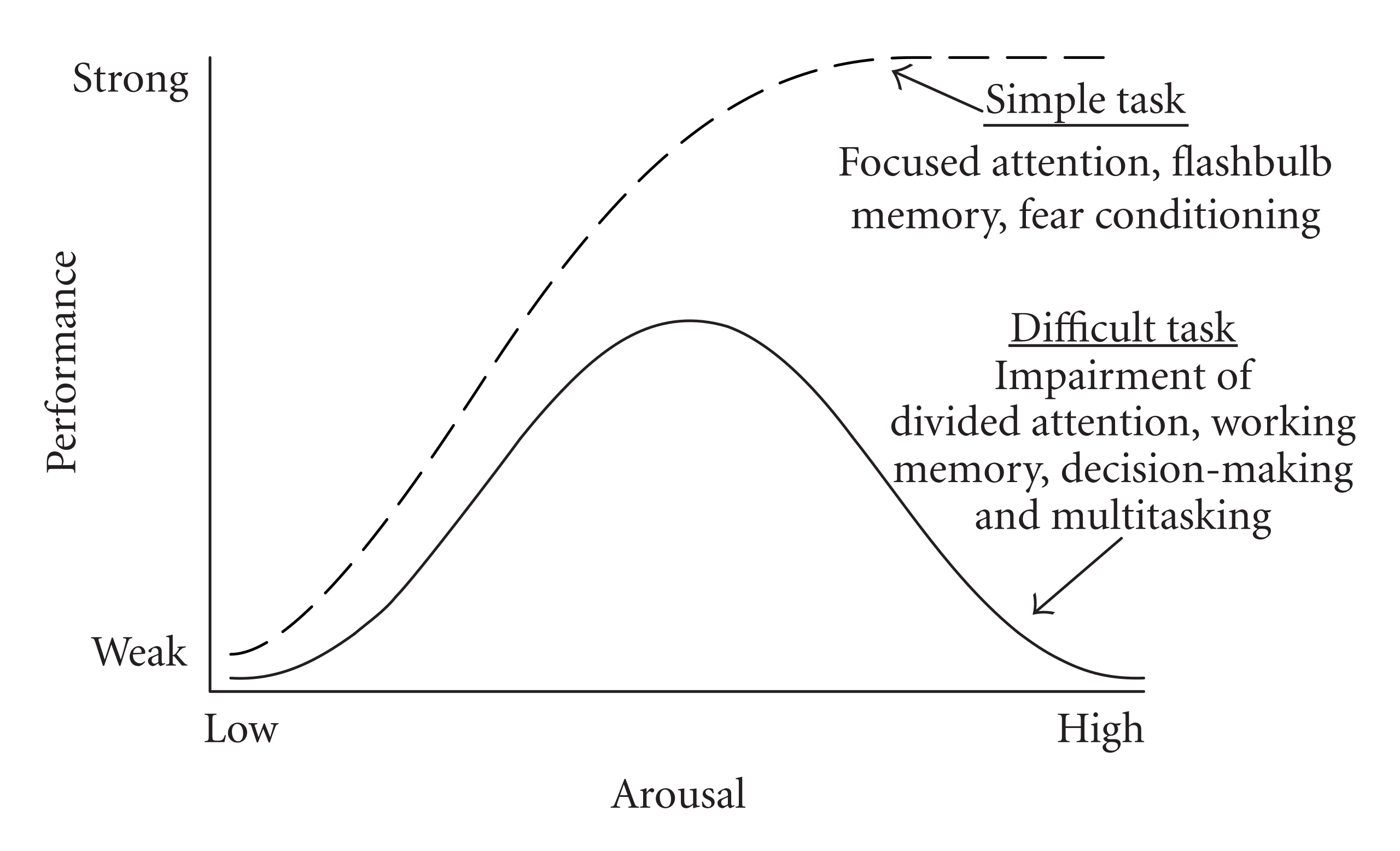
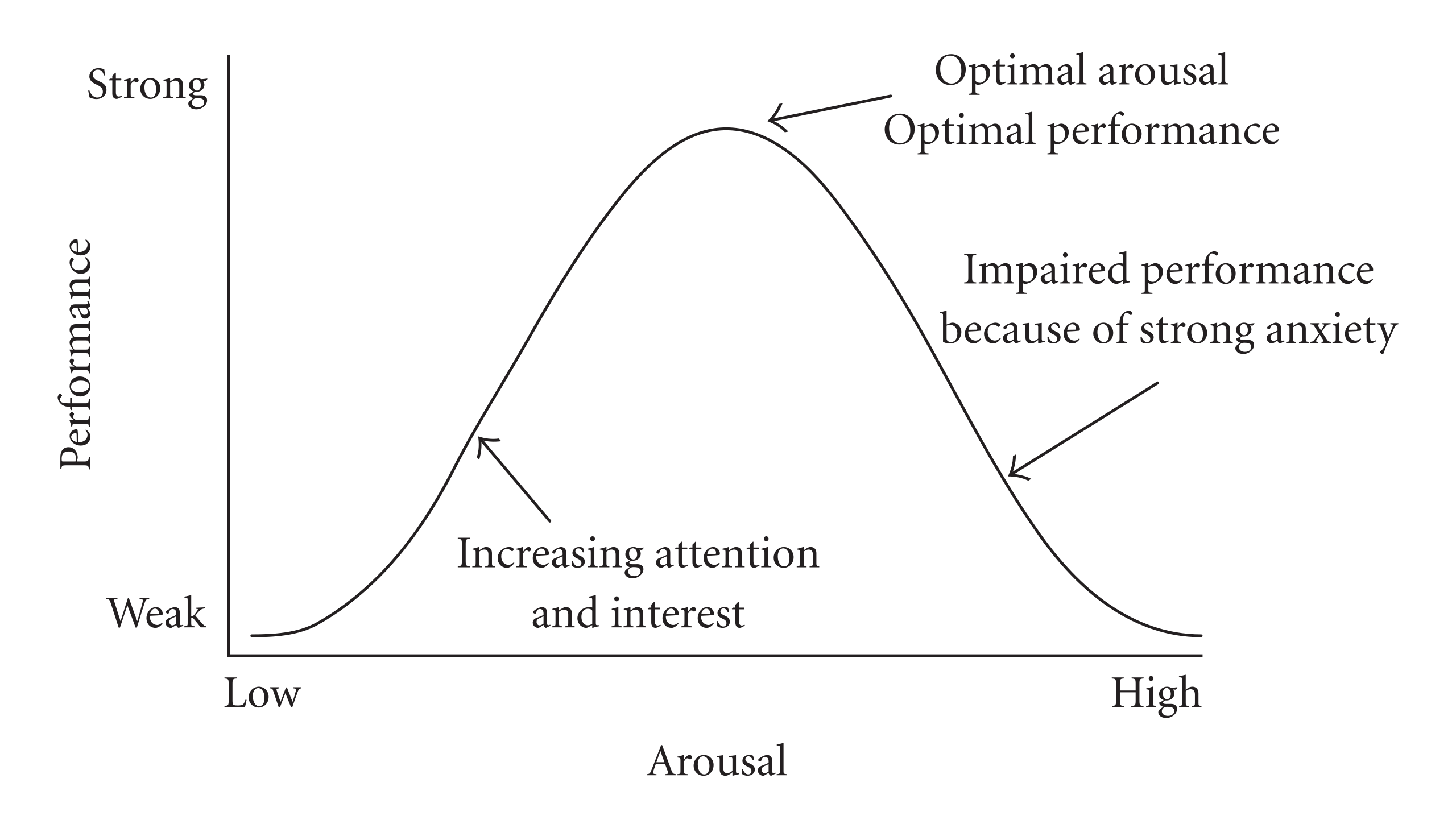
One process that may have a nonlinear association with performance is arousal or anxiety. The Yerkes–Dodson law describes the association between arousal and performance, as depicted in Figure 27.5. For simple tasks, performance tends to increase with arousal. For difficult tasks, there is an inverted-U-shaped association between arousal and performance, as depicted in Figure 27.6. For difficult tasks, too little arousal is bad because it leads to insufficient attention on the task at hand; however, too much arousal is also bad because anxiety can impair performance through its negative effects on attention (e.g., “tunnel vision”), memory, decision making, problem-solving, and multitasking. That is, there is an optimal range of arousal for complex and challenging tasks, such as those in sports, which often require divided attention and multitasking.
27.7 Expert Performance and Automaticity
This section was adapted from course materials from Motz (2018).
Automaticity involves fast and effortless processing that requires little or no focused attention. The more automatic a process is, the less likely a person is to be consciously aware of it. For instance, breathing is a fairly automatic process—people can breathe even when they are not concentrating on breathing. Chewing food can also be automatic. Automaticity helps free up resources for more demanding tasks. Football players and others often face situations requiring multitasking—i.e., performing two (or more) tasks simultaneously. For instance, a Quarterback must look for open receivers, monitor approaching defenders, move to open space when necessary, and make an accurate, well-timed throw.
Multitasking is common in everyday life, but some tasks may suffer more from divided attention than others. Driving, for example, is a complex task that may be impacted by cognitive load from secondary tasks like phone conversations. It is an important question of how well people are able to multitask. For instance, we could ask whether talking on a cell phone and driving simultaneously drains cognitive resources. If so, does talking on a phone while driving impair driving performance or conversation skills? Both tasks (conversing or driving) are highly practiced, so we might expect there to be little cost to dividing attention across these two tasks. This provides a nice opportunity to examine automaticity.
Many countries have banned hand-held cell phone use while driving. Some countries have banned all use of cell phones, including hands-free, while driving. However, states in the United States differ in their cell phone laws.
Almost all cell phone bans restrict the use of handheld cell phones while driving but do not restrict the use of hands-free devices. This is implicitly based on the assumption, from the peripheral-interference hypothesis, that any impairment to driving while talking on a cell phone is due to the use of a handheld device. However, an alternative possibility, the attentional hypothesis, posits that that driving impairment with cell phone use is due to dividing one’s attention. If this is the case, it would impact driving with both handheld and hands-free devices.
A study by Redelmeier & Tibshirani (1997) found that 25% of a sample of 699 accidents involved drives that had spoken on a cell phone within 10 minutes prior to the accident. The use of handheld and hands-free phone were equally associated with accidents suggesting divided attention is the problem, not the use of a peripheral device. However, this association was observed from a correlational design; thus, we cannot conclude that cell phone use directly caused the accidents. It may be, for instance, that risk-taking individuals or individuals in a strongly emotional state may be more likely to both a) have car accidents and b) to use cell phones while driving, which might account for such an association. Thus, we need studies to examine the effects of multitasking using experimental designs to establish causality.
Strayer & Johnston (2001) conducted an experimental study on multitasking. For the first task, the tracking task, participants tracked the position of a moving target on a computer screen. Every 10–20 seconds, the moving target flashed either red or green to simulate a traffic signal. If the target turned red (such as one might see when a traffic light turns red), the participant was supposed to push a “brake button”, which might simulate the act of needing to brake while driving. If the target turned green (such as one might see when a traffic light turns green), the participant was not supposed to do anything. During a dual-task phase, the participant was supposed to perform a second task while completing the tracking task. For the second task, participants were randomly assigned to one of four conditions: 1) conversing with an experimenter using a hand-held mobile device, 2) conversing with an experimenter using a hands-free device, 3) listening to a radio program of their choice, or 4) listening to a book on tape. The researchers found that the probability of missing a color change (i.e., a simulated traffic signal) more than doubled for the cell phone group when performing both the tracking and conversation tasks simultaneously (relative to performing only the tracking task). Reaction time also increased for the cell phone group when performing the dual tasks compared to when performing the single tracking task. However, there was no difference—in terms of the probability of missing a color change or reaction time—between the dual tasks and single task for the radio or book-on-tape control groups, suggesting that listening, by itself, does not interfere with the tracking task—rather, it appears that actively having a conversation (that includes talking and listening) interferes with tracking changes. Moreover, there was no difference between handheld or hands-free phones in terms of the probability of missing a color change or reaction time, suggesting that it was not the use of a hands-occupying device that caused their weaker performance in the tracking task—it was the act of dividing one’s attention across tasks (i.e., conversation task and tracking task) that led to weaker performance in tracking changes. Thus, the findings were consistent with the attentional hypothesis, and suggest that divided attention can interfere with performance—in addition to any deficits incurred due to peripheral factors such as handling the phone while dialing.
Many people talk on the phone while driving. What does it mean that people are (somehow) able to perform these two tasks simultaneously? It suggests that those who use the cell phone while driving are treating one of the tasks—driving—as an automatic process and not giving it focused attention. Evidence suggests that talking on the phone while driving increases the risk of accident to levels comparable to driving drunk (i.e., a blood alcohol level above the legal limit; Redelmeier & Tibshirani, 1997). The cognitive task of talking on the phone uses attentional resources that would otherwise be used for driving a car.
Strayer & Drew (2004) also replicated their findings using a driving simulator, which is a more ecologically valid assessment of driving performance than the tracking task. In the study, using the driving simulator, participants drove on a highway in both single-task (i.e., driving only) and dual-task (i.e., driving while talking on a cell phone) conditions. Participants drove while following a car that braked at various times. The authors found that use of a cell phone led drivers to show a 18% slower brake onset time, 12% greater following distance, 17% longer half-recovery time (the time to recover 50% of the speed that was lost during braking), and twice as many rear-end collisions—all despite no general differences in speed. Although older drivers were poorer overall in driving performance, the effects of cell phone use did not differ for younger (~20 years of age) and older (~70 years of age) drivers, suggesting that the driving performance for both younger and older adults is impaired by cell phone use. Indeed, the reaction time of younger drivers who were talking on a cell phone was equivalent to the reaction time of older drivers who were not using a cell phone.
The findings described above might suggest that more attention leads to better performance. Based on that assumption, we should tell a Quarterback who has thrown multiple interceptions during a game to pay more attention to his throwing mechanics when throwing the ball, right? However, it is not always the case that devoting more attention to a task leads to better performance. There are two primary competing theories for “choking” in pressure situations in sports. “Choking” refers to underperforming relative to one’s ability (Beilock & Carr, 2001).
Distraction theories posit that the pressure situation creates a distracting environment that shifts one’s attention to cues that are irrelevant to the task, such as one’s worries about the situation and its consequences (Beilock & Carr, 2001).
An alternative possibility, based on explicit monitoring theory, is that pressure situations raise one’s self-awareness and anxiety about performing well, which increases one’s attention to the step-by-step procedures involved in skill processes, which may disrupt well-learned or proceduralized performance (Beilock & Carr, 2001). Beilock & Carr (2001) found that, among automatic tasks (e.g. putting in golf among highly trained individuals), focusing too much on the task can actually hinder performance, consistent with explicit monitoring theory. For highly practiced experts, automatic skill tasks might include tasks like hitting/putting a golf ball, pitching a baseball, throwing/kicking a football, shooting free throws in basketball, shooting arrows in archery, serving in tennis, etc. Sports players often refer to highly practiced tasks as involving “muscle memory.” When a task is highly practiced or automatic, excessive attention can hurt performance. That is, more attention can lead to worse performance. This is called “choking under pressure” and is based on explicit monitoring theory.
By contrast, for tasks that require conscious control, decision-making, and real-time adjustments, more focused attention tends to lead to better performance. Tasks that require real-time adjustment include tasks such as avoiding unexpected hazards while driving or trying to avoid rushers while operating as a Quarterback. Unpredictable events occur when driving and when operating as a Quarterback; when unpredictable things happen and one’s attentions is diverted, one’s performance is likely to be impaired (Strayer & Johnston, 2001). In sum, devoting explicit attention to a task appears to improve performance when the task requires deliberate cognitive processing but can hurt performance when the task is highly automatic.
27.8 Conclusion
Football has recently seen greater use of analytics; however, its uptake has been slower compared to other sports like baseball and basketball. Examples of changes in football due to the use of analytics include more often going for it on fourth down, a greater emphasis on the passing game, drafting Running Backs later in the draft (and, more generally, valuing Running Backs less), and trading down in the draft to obtain more low picks (rather than having fewer high picks) because top picks are frequently overvalued. Historically, despite the decision hurting their chances of winning, teams rarely went for it on fourth down and elected to punt or kick a field goal instead, likely due to loss aversion bias. Loss aversion bias may lead coaches to make more conservative play-calling, in general, such as running the ball when passing would tend to be more advantageous. Rates of going for it on fourth down in the NFL were low until 2017. After the 2017 season, rates of going for it on fourth down increased dramatically. In addition to poor decisions relating to going for it on fourth down, there is not strong evidence that icing the kicker works, suggesting that it may better suit your team to use timeouts in other situations.
There are many psychological factors that influence sports performance. According to the Yerkes–Dodson law that describes the association between arousal and performance. For simple tasks, performance tends to increase with arousal. There is an optimal range of arousal for complex and challenging tasks, such as those in sports, which often require divided attention and multitasking. Too little arousal is bad because it leads to insufficient attention on the task at hand; however, too much arousal is also bad because anxiety can impair performance through its negative effects on attention (e.g., “tunnel vision”), memory, decision making, problem-solving, and multitasking. When a task is highly practiced or automatic, excessive attention can hurt performance. By contrast, for tasks that require conscious control, decision-making, and real-time adjustments, more focused attention tends to lead to better performance.
27.9 Session Info
R version 4.6.1 (2026-06-24)
Platform: x86_64-pc-linux-gnu
Running under: Ubuntu 24.04.4 LTS

Matrix products: default
BLAS:   /usr/lib/x86_64-linux-gnu/openblas-pthread/libblas.so.3
LAPACK: /usr/lib/x86_64-linux-gnu/openblas-pthread/libopenblasp-r0.3.26.so;  LAPACK version 3.12.0

locale:
 [1] LC_CTYPE=C.UTF-8       LC_NUMERIC=C           LC_TIME=C.UTF-8
 [4] LC_COLLATE=C.UTF-8     LC_MONETARY=C.UTF-8    LC_MESSAGES=C.UTF-8
 [7] LC_PAPER=C.UTF-8       LC_NAME=C              LC_ADDRESS=C
[10] LC_TELEPHONE=C         LC_MEASUREMENT=C.UTF-8 LC_IDENTIFICATION=C

time zone: UTC
tzcode source: system (glibc)

attached base packages:
[1] stats     graphics  grDevices utils     datasets  methods   base

other attached packages:
 [1] ggtext_0.1.2    lubridate_1.9.5 forcats_1.0.1   stringr_1.6.0
 [5] dplyr_1.2.1     purrr_1.2.2     readr_2.2.0     tidyr_1.3.2
 [9] tibble_3.3.1    ggplot2_4.0.3   tidyverse_2.0.0 nflreadr_1.5.1

loaded via a namespace (and not attached):
 [1] generics_0.1.4     xml2_1.6.0         stringi_1.8.7      lattice_0.22-9
 [5] hms_1.1.4          digest_0.6.39      magrittr_2.0.5     evaluate_1.0.5
 [9] grid_4.6.1         timechange_0.4.0   RColorBrewer_1.1-3 fastmap_1.2.0
[13] Matrix_1.7-5       jsonlite_2.0.0     mgcv_1.9-4         scales_1.4.0
[17] cli_3.6.6          rlang_1.3.0        litedown_0.10      commonmark_2.0.0
[21] splines_4.6.1      withr_3.0.3        cachem_1.1.0       yaml_2.3.12
[25] otel_0.2.0         tools_4.6.1        tzdb_0.5.0         memoise_2.0.1
[29] vctrs_0.7.3        R6_2.6.1           lifecycle_1.0.5    htmlwidgets_1.6.4
[33] pkgconfig_2.0.3    pillar_1.11.1      gtable_0.3.6       data.table_1.18.4
[37] glue_1.8.1         Rcpp_1.1.2         xfun_0.60          tidyselect_1.2.1
[41] knitr_1.51         farver_2.1.2       htmltools_0.5.9    nlme_3.1-169
[45] rmarkdown_2.31     labeling_0.4.3     compiler_4.6.1     S7_0.2.2
[49] markdown_2.0       gridtext_0.1.6