Code
Error in `library()`:
! there is no package called 'LongituRF'I want your feedback to make the book better for you and other readers. If you find typos, errors, or places where the text may be improved, please let me know. The best ways to provide feedback are by GitHub or hypothes.is annotations.
You can leave a comment at the bottom of the page/chapter, or open an issue or submit a pull request on GitHub: https://github.com/isaactpetersen/Fantasy-Football-Analytics-Textbook
Alternatively, you can leave an annotation using hypothes.is.
To add an annotation, select some text and then click the
symbol on the pop-up menu.
To see the annotations of others, click the
symbol in the upper right-hand corner of the page.
This chapter provides an overview of machine learning.
Error in `library()`:
! there is no package called 'LongituRF'# Downloaded Data - Processed
load(file = "./data/nfl_players.RData")
load(file = "./data/nfl_teams.RData")
load(file = "./data/nfl_rosters.RData")
load(file = "./data/nfl_rosters_weekly.RData")
load(file = "./data/nfl_schedules.RData")
load(file = "./data/nfl_combine.RData")
load(file = "./data/nfl_draftPicks.RData")
load(file = "./data/nfl_depthCharts.RData")
#load(file = "./data/nfl_pbp.RData")
#load(file = "./data/nfl_4thdown.RData")
#load(file = "./data/nfl_participation.RData")
#load(file = "./data/nfl_actualFantasyPoints_weekly.RData")
load(file = "./data/nfl_injuries.RData")
load(file = "./data/nfl_snapCounts.RData")
load(file = "./data/nfl_espnQBR_seasonal.RData")
load(file = "./data/nfl_espnQBR_weekly.RData")
load(file = "./data/nfl_nextGenStats_weekly.RData")
load(file = "./data/nfl_advancedStatsPFR_seasonal.RData")
load(file = "./data/nfl_advancedStatsPFR_weekly.RData")
load(file = "./data/nfl_playerContracts.RData")
load(file = "./data/nfl_ftnCharting.RData")
load(file = "./data/nfl_playerIDs.RData")
load(file = "./data/nfl_rankings_draft.RData")
load(file = "./data/nfl_rankings_weekly.RData")
load(file = "./data/nfl_expectedFantasyPoints_weekly.RData")
#load(file = "./data/nfl_expectedFantasyPoints_pbp.RData")
# Calculated Data - Processed
load(file = "./data/nfl_actualStats_player_career.RData")
load(file = "./data/nfl_actualStats_seasonal.RData")
load(file = "./data/player_stats_weekly.RData")
load(file = "./data/player_stats_seasonal.RData")We created the player_stats_weekly.RData and player_stats_seasonal.RData objects in Section 4.4.3.
Machine learning is a class of algorithmic approaches that are used to identify patterns in data. Machine learning takes us away from focusing on causal inference. Machine learning does not care about which processes are causal—i.e., which processes influence the outcome. Instead, machine learning cares about prediction—it cares about a predictor variable to the extent that it increases predictive accuracy regardless of whether it is causally related to the outcome. Nevertheless, association is necessary (despite being insufficient) for causality, as described in Section 13.4. Thus, achieving strong prediction is important (even if insufficient) for the model to be useful. If a model does explains only a small portion of variance, it is difficult for it to be useful.
Machine learning can be useful for leveraging big data and many predictor variables to develop predictive models with greater accuracy. However, many machine learning techniques are black boxes—it is often unclear how or why certain predictions are made, which can make it difficult to interpret the model’s decisions and understand the underlying relationships between variables. Machine learning tends to be a data-driven, atheoretical technique. This can result in overfitting. Thus, when estimating machine learning models, it is common to keep a hold-out sample for use in cross-validation to evaluate the extent of shrinkage of model coefficients. The data that the model is trained on is known as the “training data”. The data that the model was not trained on but is then is independently tested on—i.e., the hold-out sample—is the “test data”. Shrinkage occurs when predictor variables explain some random error variance in the original model. When the model is applied to an independent sample (i.e., the test data), the predictive model will likely not perform quite as well, and the regressions coefficients will tend to get smaller (i.e., shrink).
If the test data were collected as part of the same processes as the original data and were merely held out for purposes of analysis, this is called internal cross-validation. If the test data were collected separately from the original data used to train the model, this is called external cross-validation.
Although machine learning tends to be data-driven in its execution, theory should still inform which variables are included in the model.
Most machine learning methods were developed with cross-sectional data in mind. That is, they assume that each person has only one observation on the outcome variable. However, with longitudinal data, each person has multiple observations on the outcome variable.
When performing machine learning, various approaches may help address this:
There are many approaches to machine learning. This chapter discusses several key ones:
Supervised learning involves learning from data where the correct classification or outcome is known (and the classification is thus part of the data). For instance, predicting how many points a player will score is a supervised learning task, because there is a ground truth—the actual number of points scored—that can be used to train and evaluate the model. If the outcome variable is categorical, the approach involves classification. If the outcome variable is continuous, the approach involves regression.
Unlike linear and logistic regression, various machine learning techniques can handle multicollinearity, including LASSO regression, ridge regression, and elastic net regression via regularization. Regularization involves penalizing model complexity to avoid overfitting (Ramasubramanian & Singh, 2016). Least absolute shrinkage and selection option (LASSO) regression performs selection of which predictor variables to keep in the model by shrinking some coefficients to zero, effectively removing them from the model. Ridge regression shrinks the coefficients of predictor variables toward zero, but not to zero, so it does not perform selection of which predictor variables to retain; this allows it to yield stable estimates for multiple correlated predictor variables in the context of multicollinearity. Elastic net involves a combination of LASSO and ridge regression; it performs selection of which predictor variables to keep by shrinking the coefficients of some predictor variables to zero (like LASSO, for variable selection), and it shrinks the coefficients of some predictor variables toward zero (like ridge, for handling multicollinearity among correlated predictors).
Unless interactions or nonlinear terms are specified, linear, logistic, LASSO, ridge, and elastic net regression assume additive and linear associations between the predictors and outcome. That is, they do not automatically account for interactions among the predictor variables or for nonlinear associations between the predictor variables and the outcome variable (unless interaction terms or nonlinear transformations are explicitly included). By contrast, random forests and tree boosting methods automatically account for interactions and nonlinear associations between predictors and the outcome variable. These models recursively partition the data in ways that capture complex patterns without the need to manually specify interaction or polynomial terms.
Unsupervised learning involves learning from data without known classifications. Unsupervised learning is used to discover hidden patterns, groupings, or structures in the data. For instance, if we want to identify different subtypes of Wide Receivers based on their playing style or performance metrics, or uncover underlying dimensions in a large dataset, we would use an unsupervised learning approach.
We describe cluster analysis in Chapter 21. We describe factor analysis in Chapter 22. We describe principal component analysis in Chapter 23.
Semi-supervised learning combines supervised learning and unsupervised learning by training the model on some data for which the classification is known and some data for which the classification is not known.
Reinforcement learning involves an agent learning to make decisions by interacting with the environment. Through trial and error, the agent receives feedback in the form of rewards or penalties and learns a strategy that maximizes the cumulative reward over time.
Ensemble machine learning methods combine multiple machine learning approaches with the goal that combining multiple approaches might lead to more accurate predictions than any one method might be able to achieve on its own.
Several data processing steps are necessary to get the data in the form necessary for machine learning.
First, we apply several steps. We subset to the positions and variables of interest. We also rename columns and change variable types to make sure they match the column names and types across objects, which will be important later when we merge the data.
# Prepare data for merging
#nfl_actualFantasyPoints_player_weekly <- nfl_actualFantasyPoints_player_weekly %>%
# rename(gsis_id = player_id)
#
#nfl_actualFantasyPoints_player_seasonal <- nfl_actualFantasyPoints_player_seasonal %>%
# rename(gsis_id = player_id)
player_stats_seasonal_offense <- player_stats_seasonal %>%
filter(position_group %in% c("QB","RB","WR","TE")) %>%
rename(gsis_id = player_id)
player_stats_weekly_offense <- player_stats_weekly %>%
filter(position_group %in% c("QB","RB","WR","TE")) %>%
rename(gsis_id = player_id)
## Rename other variables to ensure common names
## Ensure variables with the same name have the same type
nfl_players <- nfl_players %>%
mutate(
birth_date = as.Date(birth_date),
jersey_number = as.character(jersey_number),
nfl_id = as.character(nfl_id),
years_of_experience = as.integer(years_of_experience))
player_stats_seasonal_offense <- player_stats_seasonal_offense %>%
mutate(
birth_date = as.Date(birth_date),
jersey_number = as.character(jersey_number))
nfl_rosters <- nfl_rosters %>%
mutate(
draft_number = as.integer(draft_number))
nfl_rosters_weekly <- nfl_rosters_weekly %>%
mutate(
draft_number = as.integer(draft_number))
nfl_depthCharts <- nfl_depthCharts %>%
mutate(
season = as.integer(season))
nfl_expectedFantasyPoints_weekly <- nfl_expectedFantasyPoints_weekly %>%
rename(gsis_id = player_id) %>%
mutate(
season = as.integer(season),
receptions = as.integer(receptions)) %>%
distinct(gsis_id, season, week, .keep_all = TRUE) # drop duplicated rows
## Rename variables
nfl_draftPicks <- nfl_draftPicks %>%
rename(
games_career = games,
pass_completions_career = pass_completions,
pass_attempts_career = pass_attempts,
pass_yards_career = pass_yards,
pass_tds_career = pass_tds,
pass_ints_career = pass_ints,
rush_atts_career = rush_atts,
rush_yards_career = rush_yards,
rush_tds_career = rush_tds,
receptions_career = receptions,
rec_yards_career = rec_yards,
rec_tds_career = rec_tds,
def_solo_tackles_career = def_solo_tackles,
def_ints_career = def_ints,
def_sacks_career = def_sacks
)
## Subset variables
nfl_expectedFantasyPoints_weekly <- nfl_expectedFantasyPoints_weekly %>%
select(gsis_id:position, contains("_exp"), contains("_diff"), contains("_team")) #drop "raw stats" variables (e.g., rec_yards_gained) so they don't get coalesced with actual stats
# Check duplicate ids
player_stats_seasonal_offense %>%
group_by(gsis_id, season) %>%
filter(n() > 1) %>%
head()Below, we identify shared variable names across objects to be merged to make sure we account for them in merging:
[1] "gsis_id" "position"[1] 24375[1] 11054[1] "gsis_id" "season" "team" "pfr_id" "age" [1] 15507[1] 12035[1] 15506[1] 12035[1] 15507[1] 11961[1] "gsis_id" "season" "week" "position" "full_name"[1] 888773[1] 105903[1] 888773[1] 105903[1] 888740[1] 103446[1] 888757[1] 103446To perform machine learning, we need all of the predictor variables and the outcome variable in the same data file. Thus, we must merge data files. To merge data, we use the powerjoin package (Fabri, 2022), which allows coalescing variables with the same name from two different objects. We specify coalesce_xy, which means that—for variables that have the same name across both objects—it keeps the value from object 1 (if present); if not, it keeps the value from object 2. We first merge variables from objects that have the same structure—player data (i.e., id form), seasonal data (i.e., id-season form), or weekly data (i.e., id-season-week form).
# Create lists of objects to merge, depending on data structure: id; or id-season; or id-season-week
playerListToMerge <- list(
nfl_players %>% filter(!is.na(gsis_id)),
nfl_draftPicks %>% filter(!is.na(gsis_id)) %>% select(-season)
)
playerSeasonListToMerge <- list(
player_stats_seasonal_offense %>% filter(!is.na(gsis_id), !is.na(season)),
nfl_advancedStatsPFR_seasonal %>% filter(!is.na(gsis_id), !is.na(season))
)
playerSeasonWeekListToMerge <- list(
nfl_rosters_weekly %>% filter(!is.na(gsis_id), !is.na(season), !is.na(week)),
#nfl_actualStats_offense_weekly,
nfl_expectedFantasyPoints_weekly %>% filter(!is.na(gsis_id), !is.na(season), !is.na(week))
#nfl_advancedStatsPFR_weekly,
)
playerSeasonWeekPositionListToMerge <- list(
nfl_depthCharts %>% filter(!is.na(gsis_id), !is.na(season), !is.na(week))
)
# Merge data
playerMerged <- playerListToMerge %>%
reduce(
powerjoin::power_full_join,
by = c("gsis_id"),
conflict = powerjoin::coalesce_xy) # where the objects have the same variable name (e.g., position), keep the values from object 1, unless it's NA, in which case use the relevant value from object 2
playerSeasonMerged <- playerSeasonListToMerge %>%
reduce(
powerjoin::power_full_join,
by = c("gsis_id","season"),
conflict = powerjoin::coalesce_xy) # where the objects have the same variable name (e.g., team), keep the values from object 1, unless it's NA, in which case use the relevant value from object 2
playerSeasonWeekMerged <- playerSeasonWeekListToMerge %>%
reduce(
powerjoin::power_full_join,
by = c("gsis_id","season","week"),
conflict = powerjoin::coalesce_xy) # where the objects have the same variable name (e.g., position), keep the values from object 1, unless it's NA, in which case use the relevant value from object 2To prepare for merging player data with seasonal data, we identify shared variable names across the objects:
[1] "gsis_id" "position"
[3] "position_group" "display_name"
[5] "common_first_name" "first_name"
[7] "last_name" "short_name"
[9] "football_name" "suffix"
[11] "esb_id" "nfl_id"
[13] "pff_id" "otc_id"
[15] "espn_id" "smart_id"
[17] "birth_date" "ngs_position_group"
[19] "ngs_position" "height"
[21] "weight" "headshot"
[23] "college_name" "college_conference"
[25] "jersey_number" "rookie_season"
[27] "last_season" "status"
[29] "ngs_status" "ngs_status_short_description"
[31] "pff_position" "pff_status"
[33] "draft_year" "draft_round"
[35] "draft_pick" "draft_team"
[37] "years_of_experience" "pfr_player_name"
[39] "team" "pfr_id"
[41] "age" Then we merge the player data with the seasonal data:
seasonalData <- powerjoin::power_full_join(
playerSeasonMerged,
playerMerged %>% select(-age, -years_of_experience, -team, -latest_team, -last_season, -pff_status), # drop variables from id objects that change from year to year (and thus are not necessarily accurate for a given season)
by = "gsis_id",
conflict = powerjoin::coalesce_xy # where the objects have the same variable name (e.g., position), keep the values from object 1, unless it's NA, in which case use the relevant value from object 2
) %>%
filter(!is.na(season)) %>%
select(gsis_id, season, player_display_name, position, team, games, everything())To prepare for merging player and seasonal data with weekly data, we identify shared variable names across the objects:
[1] "gsis_id" "season" "week" "team"
[5] "jersey_number" "status" "first_name" "last_name"
[9] "birth_date" "height" "weight" "college"
[13] "espn_id" "pff_id" "pfr_id" "headshot_url"
[17] "ngs_position" "football_name" "esb_id" "smart_id"
[21] "position" Then we merge the player and seasonal data with the weekly data:
seasonalAndWeeklyData <- powerjoin::power_full_join(
playerSeasonWeekMerged,
seasonalData,
by = c("gsis_id","season"),
conflict = powerjoin::coalesce_xy # where the objects have the same variable name (e.g., position), keep the values from object 1, unless it's NA, in which case use the relevant value from object 2
) %>%
filter(!is.na(week)) %>%
select(gsis_id, season, week, full_name, position, team, everything())For purposes of machine learning, we set all character and logical columns to factors.
For variables that are not expected to change, such as a player’s name and position, we fill in missing values by using a player’s value on those variables from other rows in the data.
We create a new data object that contains the latest seasonal data, for merging with later predictions.
To develop a machine learning model that uses a player’s performance metrics in a given season for predicting the player’s fantasy points in the subsequent season, we need to include the player’s fantasy points from the subsequent season in the same row as the previous season’s performance metrics. Thus, we need to create a lagged variable for fantasy points. That way, 2024 fantasy points are in the same row as 2023 performance metrics, 2023 fantasy points are in the same row as 2023 performance metrics, and so on. We call this the lagged fantasy points variable (fantasyPoints_lag). We also retain the original same-year fantasy points variable (fantasyPoints) so it can be used as predictor of their subsequent-year fantasy points.
Then, we drop variables that we do not want to include in the model as our predictor or outcome variable. Thus, all of the variables in the object are our predictor and outcome variables.
dropVars <- c(
"birth_date", "player_display_name", "team", "player_name", "headshot_url", "season_type", "fg_made_list", "fg_missed_list", "fg_blocked_list", "gwfg_distance_list", "pff_status", "startdate", "pos", "merge_name", "pfr_player_id", "cfb_player_id", "hof", "category", "side", "college", "car_av", "display_name", "common_first_name", "first_name", "last_name", "short_name", "football_name", "suffix", "esb_id", "nfl_id", "pff_id", "otc_id", "espn_id", "smart_id", "ngs_position_group", "ngs_position", "headshot", "college_name", "college_conference", "jersey_number", "status", "ngs_status", "ngs_status_short_description", "pff_position", "draft_team", "pfr_player_name", "pfr_id")
seasonalData_lag_subset <- seasonalData_lag %>%
dplyr::select(-any_of(dropVars))Then, we separate the objects by position, so we can develop different machine learning models for each position.
seasonalData_lag_subsetQB <- seasonalData_lag_subset %>%
filter(position == "QB") %>%
select(
gsis_id, season, games, gs, years_of_experience, age, ageCentered20, ageCentered20Quadratic,
height, weight, rookie_season, draft_pick,
fantasy_points, fantasy_points_ppr, fantasyPoints, fantasyPoints_lag,
completions:rushing_2pt_conversions, special_teams_tds, contains(".pass"), contains(".rush"))
seasonalData_lag_subsetRB <- seasonalData_lag_subset %>%
filter(position == "RB") %>%
select(
gsis_id, season, games, gs, years_of_experience, age, ageCentered20, ageCentered20Quadratic,
height, weight, rookie_season, draft_pick,
fantasy_points, fantasy_points_ppr, fantasyPoints, fantasyPoints_lag,
carries:special_teams_tds, contains(".rush"), contains(".rec"))
seasonalData_lag_subsetWR <- seasonalData_lag_subset %>%
filter(position == "WR") %>%
select(
gsis_id, season, games, gs, years_of_experience, age, ageCentered20, ageCentered20Quadratic,
height, weight, rookie_season, draft_pick,
fantasy_points, fantasy_points_ppr, fantasyPoints, fantasyPoints_lag,
carries:special_teams_tds, contains(".rush"), contains(".rec"))
seasonalData_lag_subsetTE <- seasonalData_lag_subset %>%
filter(position == "TE") %>%
select(
gsis_id, season, games, gs, years_of_experience, age, ageCentered20, ageCentered20Quadratic,
height, weight, rookie_season, draft_pick,
fantasy_points, fantasy_points_ppr, fantasyPoints, fantasyPoints_lag,
carries:special_teams_tds, contains(".rush"), contains(".rec"))Because machine learning can leverage many predictors, it is at high risk of overfitting—explaining error variance that would not generalize to new data, such as data for new players or future seasons. Thus, it is important to develop and tune the machine learning model so as not to overfit the model. In machine learning, it is common to use cross-validation where we train the model on a subset of the observations, and we evaluate how well the model generalizes to unseen (e.g., “hold-out”) observations. Then, we select the model parameters by how well the model generalizes to the hold-out data, so we are selecting a model that maximizes accuracy and generalizability (i.e., parsimony).
For internal cross-validation, it is common to divide the data into three subsets:
The training set is used to fit the model. It is usually the largest portion of the data. We fit various models to the training set based on which parameters we want to evaluate (e.g., how many trees to use in a gradient tree boosting model).
The models fit with the training set are then evaluated using the unseen observations in the validation set. The validation set is used to tune the model parameters and prevent overfitting. We select the model parameters that yield the greatest accuracy in the validation set. In k-fold cross-validation, the validation set rotates across folds, thus replacing the need for a separate validation set.
The test set is used after model training and tuning to evaluate the model’s generalizability to unseen data.
Below, we split the data into test and training data. Our ultimate goal is to predict next year’s fantasy points. However, to do that effectively, we must first develop a model for which we can evaluate its accuracy against historical fantasy points (because we do not yet know players will score in the future). We want to include all current/active players in our training data, so that our predictions of their future performance can be accounted for by including their prior data in the model. Thus, we use retired players as our hold-out (test) data. We split our data into 80% training data and 20% testing data. The 20% testing data thus includes all retired players, but not all retired players are in the testing data.
Then, for the analysis, we can either a) use rotating folds (as the case for k-fold and leave-one-out [LOO] cross-validation) for which a separate validation set (from the training set) is not needed, as we do in Section 19.6, or we can b) subdivide the training set into an inner training set and validation set, as we do in Section 19.8.5.4.
seasonalData_lag_qb_all <- seasonalData_lag_subsetQB
seasonalData_lag_rb_all <- seasonalData_lag_subsetRB
seasonalData_lag_wr_all <- seasonalData_lag_subsetWR
seasonalData_lag_te_all <- seasonalData_lag_subsetTE
set.seed(52242) # for reproducibility (to keep the same train/holdout players)
activeQBs <- unique(seasonalData_lag_qb_all$gsis_id[which(seasonalData_lag_qb_all$season == max(seasonalData_lag_qb_all$season, na.rm = TRUE))])
retiredQBs <- unique(seasonalData_lag_qb_all$gsis_id[which(seasonalData_lag_qb_all$gsis_id %ni% activeQBs)])
numQBs <- length(unique(seasonalData_lag_qb_all$gsis_id))
qbHoldoutIDs <- sample(retiredQBs, size = ceiling(.2 * numQBs)) # holdout 20% of players
activeRBs <- unique(seasonalData_lag_rb_all$gsis_id[which(seasonalData_lag_rb_all$season == max(seasonalData_lag_rb_all$season, na.rm = TRUE))])
retiredRBs <- unique(seasonalData_lag_rb_all$gsis_id[which(seasonalData_lag_rb_all$gsis_id %ni% activeRBs)])
numRBs <- length(unique(seasonalData_lag_rb_all$gsis_id))
rbHoldoutIDs <- sample(retiredRBs, size = ceiling(.2 * numRBs)) # holdout 20% of players
set.seed(52242) # for reproducibility (to keep the same train/holdout players); added here to prevent a downstream error with predict.missRanger() due to missingness; this suggests that an error can arise from including a player in the holdout sample who has missingness in particular variables; would be good to identify which player(s) in the holdout sample evoke that error to identify the kinds of missingness that yield the error
activeWRs <- unique(seasonalData_lag_wr_all$gsis_id[which(seasonalData_lag_wr_all$season == max(seasonalData_lag_wr_all$season, na.rm = TRUE))])
retiredWRs <- unique(seasonalData_lag_wr_all$gsis_id[which(seasonalData_lag_wr_all$gsis_id %ni% activeWRs)])
numWRs <- length(unique(seasonalData_lag_wr_all$gsis_id))
wrHoldoutIDs <- sample(retiredWRs, size = ceiling(.2 * numWRs)) # holdout 20% of players
activeTEs <- unique(seasonalData_lag_te_all$gsis_id[which(seasonalData_lag_te_all$season == max(seasonalData_lag_te_all$season, na.rm = TRUE))])
retiredTEs <- unique(seasonalData_lag_te_all$gsis_id[which(seasonalData_lag_te_all$gsis_id %ni% activeTEs)])
numTEs <- length(unique(seasonalData_lag_te_all$gsis_id))
teHoldoutIDs <- sample(retiredTEs, size = ceiling(.2 * numTEs)) # holdout 20% of players
seasonalData_lag_qb_train <- seasonalData_lag_qb_all %>%
filter(gsis_id %ni% qbHoldoutIDs)
seasonalData_lag_qb_test <- seasonalData_lag_qb_all %>%
filter(gsis_id %in% qbHoldoutIDs)
seasonalData_lag_rb_train <- seasonalData_lag_rb_all %>%
filter(gsis_id %ni% rbHoldoutIDs)
seasonalData_lag_rb_test <- seasonalData_lag_rb_all %>%
filter(gsis_id %in% rbHoldoutIDs)
seasonalData_lag_wr_train <- seasonalData_lag_wr_all %>%
filter(gsis_id %ni% wrHoldoutIDs)
seasonalData_lag_wr_test <- seasonalData_lag_wr_all %>%
filter(gsis_id %in% wrHoldoutIDs)
seasonalData_lag_te_train <- seasonalData_lag_te_all %>%
filter(gsis_id %ni% teHoldoutIDs)
seasonalData_lag_te_test <- seasonalData_lag_te_all %>%
filter(gsis_id %in% teHoldoutIDs)Many of the machine learning approaches described in this chapter require no missing observations in order for a case to be included in the analysis. In this section, we demonstrate one approach to imputing missing data. Here is a vignette demonstrating how to impute missing data using missForest(): https://rpubs.com/lmorgan95/MissForest (archived at: https://perma.cc/6GB4-2E22). Below, we impute the training data (and all data) separately by position. We then use the imputed training data to make out-of-sample predictions to fill in the missing data for the testing data. We do not want to impute the training and testing data together so that we can keep them separate for the purposes of cross-validation. However, we impute all data (training and test data together) for purposes of making out-of-sample predictions from the machine learning models to predict players’ performance next season (when actuals are not yet available for evaluating their accuracy). To impute data, we use the missRanger package (Mayer, 2024).
Note: the following code takes a while to run.
Skip constant features for imputation: special_teams_tds
Variables to impute: passing_epa, pacr, rushing_epa, draft_pick, fantasyPoints_lag, passing_cpoe, gs, pass_attempts.pass, throwaways.pass, spikes.pass, drops.pass, bad_throws.pass, times_blitzed.pass, times_hurried.pass, times_hit.pass, times_pressured.pass, batted_balls.pass, on_tgt_throws.pass, rpo_plays.pass, rpo_yards.pass, rpo_pass_att.pass, rpo_pass_yards.pass, rpo_rush_att.pass, rpo_rush_yards.pass, pa_pass_att.pass, pa_pass_yards.pass, intended_air_yards.pass, intended_air_yards_per_pass_attempt.pass, completed_air_yards.pass, completed_air_yards_per_completion.pass, completed_air_yards_per_pass_attempt.pass, pass_yards_after_catch.pass, pass_yards_after_catch_per_completion.pass, scrambles.pass, scramble_yards_per_attempt.pass, att.rush, yds.rush, td.rush, x1d.rush, ybc.rush, yac.rush, brk_tkl.rush, att_br.rush, ybc_att.rush, yac_att.rush, drop_pct.pass, bad_throw_pct.pass, on_tgt_pct.pass, pressure_pct.pass, pocket_time.pass
Variables used to impute: gsis_id, season, games, gs, years_of_experience, age, ageCentered20, ageCentered20Quadratic, height, weight, rookie_season, draft_pick, fantasy_points, fantasy_points_ppr, fantasyPoints, fantasyPoints_lag, completions, attempts, passing_yards, passing_tds, passing_interceptions, sacks_suffered, sack_yards_lost, sack_fumbles, sack_fumbles_lost, passing_air_yards, passing_yards_after_catch, passing_first_downs, passing_epa, passing_cpoe, passing_2pt_conversions, pacr, carries, rushing_yards, rushing_tds, rushing_fumbles, rushing_fumbles_lost, rushing_first_downs, rushing_epa, rushing_2pt_conversions, pocket_time.pass, pass_attempts.pass, throwaways.pass, spikes.pass, drops.pass, bad_throws.pass, times_blitzed.pass, times_hurried.pass, times_hit.pass, times_pressured.pass, batted_balls.pass, on_tgt_throws.pass, rpo_plays.pass, rpo_yards.pass, rpo_pass_att.pass, rpo_pass_yards.pass, rpo_rush_att.pass, rpo_rush_yards.pass, pa_pass_att.pass, pa_pass_yards.pass, intended_air_yards.pass, intended_air_yards_per_pass_attempt.pass, completed_air_yards.pass, completed_air_yards_per_completion.pass, completed_air_yards_per_pass_attempt.pass, pass_yards_after_catch.pass, pass_yards_after_catch_per_completion.pass, scrambles.pass, scramble_yards_per_attempt.pass, drop_pct.pass, bad_throw_pct.pass, on_tgt_pct.pass, pressure_pct.pass, ybc_att.rush, yac_att.rush, att.rush, yds.rush, td.rush, x1d.rush, ybc.rush, yac.rush, brk_tkl.rush, att_br.rush
pssng_p pacr rshng_ drft_p fntsP_ pssng_c gs pss_t. thrww. spks.p drps.p bd_th. tms_b. tms_hr. tms_ht. tms_p. bttd_. on_tgt_t. rp_pl. rp_yr. rp_pss_t. rp_pss_y. rp_rsh_t. rp_rsh_y. p_pss_t. p_pss_y. int__. i_____ cmp__. c____. c_____ ps___. p_____ scrmb. sc___. att.rs yds.rs td.rsh x1d.rs ybc.rs yc.rsh brk_t. att_b. ybc_t. yc_tt. drp_p. bd_t_. on_tgt_p. prss_. pckt_.
iter 1: 0.1907 0.7673 0.3568 0.6181 0.4790 0.4172 0.0176 0.0103 0.2858 0.7426 0.1242 0.0476 0.0643 0.1640 0.1700 0.0340 0.2910 0.0223 0.2555 0.1498 0.0740 0.0688 0.2632 0.2499 0.1758 0.0937 0.0451 0.1297 0.0319 0.1976 0.1271 0.0226 0.1383 0.0772 0.1403 0.0353 0.0434 0.1677 0.0377 0.0492 0.1651 0.3620 0.3634 0.2942 0.5329 0.7202 0.4802 0.1082 0.6224 0.7345
iter 2: 0.1959 0.7982 0.3493 0.6960 0.4855 0.3995 0.0167 0.0088 0.2677 0.7225 0.0705 0.0327 0.0615 0.1172 0.1239 0.0279 0.2666 0.0107 0.0517 0.0694 0.0614 0.0817 0.1940 0.2788 0.0531 0.0705 0.0200 0.0917 0.0223 0.1419 0.1172 0.0195 0.1463 0.0667 0.1284 0.0236 0.0273 0.1666 0.0377 0.0398 0.1131 0.2301 0.3443 0.2867 0.5283 0.6697 0.4726 0.1061 0.6122 0.7352
iter 3: 0.1929 0.8052 0.3539 0.6963 0.4831 0.4022 0.0165 0.0088 0.2732 0.7260 0.0691 0.0339 0.0616 0.1170 0.1251 0.0277 0.2623 0.0107 0.0512 0.0686 0.0606 0.0822 0.2044 0.2739 0.0527 0.0707 0.0198 0.0946 0.0220 0.1498 0.1274 0.0207 0.1428 0.0658 0.1288 0.0248 0.0273 0.1722 0.0364 0.0399 0.1171 0.2360 0.3546 0.2909 0.5389 0.6839 0.4639 0.1044 0.6014 0.7382 missRanger object. Extract imputed data via $data
- best iteration: 2
- best average OOB imputation error: 0.2131781 data_all_qb <- seasonalData_lag_qb_all_imp$data
data_all_qb$fantasyPointsMC_lag <- scale(data_all_qb$fantasyPoints_lag, scale = FALSE) # mean-centered
data_all_qb_matrix <- data_all_qb %>%
mutate(across(where(is.factor), ~ as.numeric(as.integer(.)))) %>%
as.matrix()
newData_qb <- data_all_qb %>%
filter(season == max(season, na.rm = TRUE)) %>%
select(-fantasyPoints_lag, -fantasyPointsMC_lag)
newData_qb_matrix <- data_all_qb_matrix[
data_all_qb_matrix[, "season"] == max(data_all_qb_matrix[, "season"], na.rm = TRUE), # keep only rows with the most recent season
, # all columns
drop = FALSE]
dropCol_qb <- which(colnames(newData_qb_matrix) %in% c("fantasyPoints_lag","fantasyPointsMC_lag"))
newData_qb_matrix <- newData_qb_matrix[, -dropCol_qb, drop = FALSE]
seasonalData_lag_qb_train_imp <- missRanger::missRanger(
seasonalData_lag_qb_train,
pmm.k = 5,
verbose = 2,
seed = 52242,
keep_forests = TRUE)
Skip constant features for imputation: special_teams_tds
Variables to impute: passing_epa, pacr, rushing_epa, draft_pick, fantasyPoints_lag, passing_cpoe, gs, pass_attempts.pass, throwaways.pass, spikes.pass, drops.pass, bad_throws.pass, times_blitzed.pass, times_hurried.pass, times_hit.pass, times_pressured.pass, batted_balls.pass, on_tgt_throws.pass, rpo_plays.pass, rpo_yards.pass, rpo_pass_att.pass, rpo_pass_yards.pass, rpo_rush_att.pass, rpo_rush_yards.pass, pa_pass_att.pass, pa_pass_yards.pass, intended_air_yards.pass, intended_air_yards_per_pass_attempt.pass, completed_air_yards.pass, completed_air_yards_per_completion.pass, completed_air_yards_per_pass_attempt.pass, pass_yards_after_catch.pass, pass_yards_after_catch_per_completion.pass, scrambles.pass, scramble_yards_per_attempt.pass, att.rush, yds.rush, td.rush, x1d.rush, ybc.rush, yac.rush, brk_tkl.rush, att_br.rush, ybc_att.rush, yac_att.rush, drop_pct.pass, bad_throw_pct.pass, on_tgt_pct.pass, pressure_pct.pass, pocket_time.pass
Variables used to impute: gsis_id, season, games, gs, years_of_experience, age, ageCentered20, ageCentered20Quadratic, height, weight, rookie_season, draft_pick, fantasy_points, fantasy_points_ppr, fantasyPoints, fantasyPoints_lag, completions, attempts, passing_yards, passing_tds, passing_interceptions, sacks_suffered, sack_yards_lost, sack_fumbles, sack_fumbles_lost, passing_air_yards, passing_yards_after_catch, passing_first_downs, passing_epa, passing_cpoe, passing_2pt_conversions, pacr, carries, rushing_yards, rushing_tds, rushing_fumbles, rushing_fumbles_lost, rushing_first_downs, rushing_epa, rushing_2pt_conversions, pocket_time.pass, pass_attempts.pass, throwaways.pass, spikes.pass, drops.pass, bad_throws.pass, times_blitzed.pass, times_hurried.pass, times_hit.pass, times_pressured.pass, batted_balls.pass, on_tgt_throws.pass, rpo_plays.pass, rpo_yards.pass, rpo_pass_att.pass, rpo_pass_yards.pass, rpo_rush_att.pass, rpo_rush_yards.pass, pa_pass_att.pass, pa_pass_yards.pass, intended_air_yards.pass, intended_air_yards_per_pass_attempt.pass, completed_air_yards.pass, completed_air_yards_per_completion.pass, completed_air_yards_per_pass_attempt.pass, pass_yards_after_catch.pass, pass_yards_after_catch_per_completion.pass, scrambles.pass, scramble_yards_per_attempt.pass, drop_pct.pass, bad_throw_pct.pass, on_tgt_pct.pass, pressure_pct.pass, ybc_att.rush, yac_att.rush, att.rush, yds.rush, td.rush, x1d.rush, ybc.rush, yac.rush, brk_tkl.rush, att_br.rush
pssng_p pacr rshng_ drft_p fntsP_ pssng_c gs pss_t. thrww. spks.p drps.p bd_th. tms_b. tms_hr. tms_ht. tms_p. bttd_. on_tgt_t. rp_pl. rp_yr. rp_pss_t. rp_pss_y. rp_rsh_t. rp_rsh_y. p_pss_t. p_pss_y. int__. i_____ cmp__. c____. c_____ ps___. p_____ scrmb. sc___. att.rs yds.rs td.rsh x1d.rs ybc.rs yc.rsh brk_t. att_b. ybc_t. yc_tt. drp_p. bd_t_. on_tgt_p. prss_. pckt_.
iter 1: 0.1913 0.5368 0.3657 0.6060 0.4784 0.4428 0.0177 0.0105 0.2885 0.7528 0.1316 0.0469 0.0659 0.1672 0.1761 0.0352 0.2995 0.0233 0.2636 0.1571 0.0742 0.0717 0.2416 0.2372 0.1609 0.0881 0.0461 0.1323 0.0285 0.1958 0.1190 0.0225 0.1369 0.0832 0.1399 0.0354 0.0473 0.1777 0.0375 0.0496 0.1694 0.3665 0.3728 0.3059 0.5611 0.6831 0.5167 0.1157 0.6071 0.7465
iter 2: 0.1974 0.5666 0.3560 0.6927 0.4938 0.4146 0.0171 0.0095 0.2743 0.7299 0.0714 0.0350 0.0634 0.1180 0.1254 0.0284 0.2736 0.0122 0.0516 0.0700 0.0623 0.0855 0.1912 0.2847 0.0538 0.0647 0.0194 0.0972 0.0231 0.1545 0.1212 0.0203 0.1432 0.0637 0.1275 0.0252 0.0276 0.1878 0.0387 0.0418 0.1117 0.2536 0.3576 0.3080 0.5464 0.7128 0.4666 0.1107 0.6270 0.7543
iter 3: 0.1993 0.5556 0.3594 0.6945 0.4912 0.4115 0.0165 0.0093 0.2754 0.7359 0.0726 0.0345 0.0634 0.1172 0.1283 0.0287 0.2701 0.0115 0.0496 0.0681 0.0627 0.0839 0.1995 0.2953 0.0559 0.0680 0.0206 0.0989 0.0203 0.1464 0.1215 0.0205 0.1437 0.0661 0.1248 0.0253 0.0275 0.1818 0.0384 0.0427 0.1178 0.2479 0.3692 0.3069 0.5602 0.6900 0.4713 0.1093 0.6510 0.7440 missRanger object. Extract imputed data via $data
- best iteration: 2
- best average OOB imputation error: 0.2136606 data_train_qb <- seasonalData_lag_qb_train_imp$data
data_train_qb$fantasyPointsMC_lag <- scale(data_train_qb$fantasyPoints_lag, scale = FALSE) # mean-centered
data_train_qb_matrix <- data_train_qb %>%
mutate(across(where(is.factor), ~ as.numeric(as.integer(.)))) %>%
as.matrix()
seasonalData_lag_qb_test_imp <- predict(
object = seasonalData_lag_qb_train_imp,
newdata = seasonalData_lag_qb_test,
seed = 52242)
data_test_qb <- seasonalData_lag_qb_test_imp
data_test_qb_matrix <- data_test_qb %>%
mutate(across(where(is.factor), ~ as.numeric(as.integer(.)))) %>%
as.matrix()# RBs
seasonalData_lag_rb_all_imp <- missRanger::missRanger(
seasonalData_lag_rb_all,
pmm.k = 5,
verbose = 2,
seed = 52242,
keep_forests = TRUE)
seasonalData_lag_rb_all_imp
data_all_rb <- seasonalData_lag_rb_all_imp$data
data_all_rb$fantasyPointsMC_lag <- scale(data_all_rb$fantasyPoints_lag, scale = FALSE) # mean-centered
data_all_rb_matrix <- data_all_rb %>%
mutate(across(where(is.factor), ~ as.numeric(as.integer(.)))) %>%
as.matrix()
newData_rb <- data_all_rb %>%
filter(season == max(season, na.rm = TRUE)) %>%
select(-fantasyPoints_lag, -fantasyPointsMC_lag)
newData_rb_matrix <- data_all_rb_matrix[
data_all_rb_matrix[, "season"] == max(data_all_rb_matrix[, "season"], na.rm = TRUE), # keep only rows with the most recent season
, # all columns
drop = FALSE]
dropCol_rb <- which(colnames(newData_rb_matrix) %in% c("fantasyPoints_lag","fantasyPointsMC_lag"))
newData_rb_matrix <- newData_rb_matrix[, -dropCol_rb, drop = FALSE]
seasonalData_lag_rb_train_imp <- missRanger::missRanger(
seasonalData_lag_rb_train,
pmm.k = 5,
verbose = 2,
seed = 52242,
keep_forests = TRUE)
seasonalData_lag_rb_train_imp
data_train_rb <- seasonalData_lag_rb_train_imp$data
data_train_rb$fantasyPointsMC_lag <- scale(data_train_rb$fantasyPoints_lag, scale = FALSE) # mean-centered
data_train_rb_matrix <- data_train_rb %>%
mutate(across(where(is.factor), ~ as.numeric(as.integer(.)))) %>%
as.matrix()
seasonalData_lag_rb_test_imp <- predict(
object = seasonalData_lag_rb_train_imp,
newdata = seasonalData_lag_rb_test,
seed = 52242)
data_test_rb <- seasonalData_lag_rb_test_imp
data_test_rb_matrix <- data_test_rb %>%
mutate(across(where(is.factor), ~ as.numeric(as.integer(.)))) %>%
as.matrix()# WRs
seasonalData_lag_wr_all_imp <- missRanger::missRanger(
seasonalData_lag_wr_all,
pmm.k = 5,
verbose = 2,
seed = 52242,
keep_forests = TRUE)
seasonalData_lag_wr_all_imp
data_all_wr <- seasonalData_lag_wr_all_imp$data
data_all_wr$fantasyPointsMC_lag <- scale(data_all_wr$fantasyPoints_lag, scale = FALSE) # mean-centered
data_all_wr_matrix <- data_all_wr %>%
mutate(across(where(is.factor), ~ as.numeric(as.integer(.)))) %>%
as.matrix()
newData_wr <- data_all_wr %>%
filter(season == max(season, na.rm = TRUE)) %>%
select(-fantasyPoints_lag, -fantasyPointsMC_lag)
newData_wr_matrix <- data_all_wr_matrix[
data_all_wr_matrix[, "season"] == max(data_all_wr_matrix[, "season"], na.rm = TRUE), # keep only rows with the most recent season
, # all columns
drop = FALSE]
dropCol_wr <- which(colnames(newData_wr_matrix) %in% c("fantasyPoints_lag","fantasyPointsMC_lag"))
newData_wr_matrix <- newData_wr_matrix[, -dropCol_wr, drop = FALSE]
seasonalData_lag_wr_train_imp <- missRanger::missRanger(
seasonalData_lag_wr_train,
pmm.k = 5,
verbose = 2,
seed = 52242,
keep_forests = TRUE)
seasonalData_lag_wr_train_imp
data_train_wr <- seasonalData_lag_wr_train_imp$data
data_train_wr$fantasyPointsMC_lag <- scale(data_train_wr$fantasyPoints_lag, scale = FALSE) # mean-centered
data_train_wr_matrix <- data_train_wr %>%
mutate(across(where(is.factor), ~ as.numeric(as.integer(.)))) %>%
as.matrix()
seasonalData_lag_wr_test_imp <- predict(
object = seasonalData_lag_wr_train_imp,
newdata = seasonalData_lag_wr_test,
seed = 52242)
data_test_wr <- seasonalData_lag_wr_test_imp
data_test_wr_matrix <- data_test_wr %>%
mutate(across(where(is.factor), ~ as.numeric(as.integer(.)))) %>%
as.matrix()# TEs
seasonalData_lag_te_all_imp <- missRanger::missRanger(
seasonalData_lag_te_all,
pmm.k = 5,
verbose = 2,
seed = 52242,
keep_forests = TRUE)
seasonalData_lag_te_all_imp
data_all_te <- seasonalData_lag_te_all_imp$data
data_all_te$fantasyPointsMC_lag <- scale(data_all_te$fantasyPoints_lag, scale = FALSE) # mean-centered
data_all_te_matrix <- data_all_te %>%
mutate(across(where(is.factor), ~ as.numeric(as.integer(.)))) %>%
as.matrix()
newData_te <- data_all_te %>%
filter(season == max(season, na.rm = TRUE)) %>%
select(-fantasyPoints_lag, -fantasyPointsMC_lag)
newData_te_matrix <- data_all_te_matrix[
data_all_te_matrix[, "season"] == max(data_all_te_matrix[, "season"], na.rm = TRUE), # keep only rows with the most recent season
, # all columns
drop = FALSE]
dropCol_te <- which(colnames(newData_te_matrix) %in% c("fantasyPoints_lag","fantasyPointsMC_lag"))
newData_te_matrix <- newData_te_matrix[, -dropCol_te, drop = FALSE]
seasonalData_lag_te_train_imp <- missRanger::missRanger(
seasonalData_lag_te_train,
pmm.k = 5,
verbose = 2,
seed = 52242,
keep_forests = TRUE)
seasonalData_lag_te_train_imp
data_train_te <- seasonalData_lag_te_train_imp$data
data_train_te$fantasyPointsMC_lag <- scale(data_train_te$fantasyPoints_lag, scale = FALSE) # mean-centered
data_train_te_matrix <- data_train_te %>%
mutate(across(where(is.factor), ~ as.numeric(as.integer(.)))) %>%
as.matrix()
seasonalData_lag_te_test_imp <- predict(
object = seasonalData_lag_te_train_imp,
newdata = seasonalData_lag_te_test,
seed = 52242)
data_test_te <- seasonalData_lag_te_test_imp
data_test_te_matrix <- data_test_te %>%
mutate(across(where(is.factor), ~ as.numeric(as.integer(.)))) %>%
as.matrix()We use the future package (Bengtsson, 2025) for parallel (faster) processing.
In the examples below, we predict the future fantasy points of Quarterbacks. However, the examples could be applied to any of the positions. There are various approaches to cross-validation. In the examples below, we use k-fold cross-validation. However, we also provide the code to apply leave-one-out (LOO) cross-validation. k-fold and LOO cross-validation are both forms of internal cross-validation.
k-fold cross-validation partitions the data into k folds (subsets). In each of the k iterations, the model is trained on \(k - 1\) folds and is evaluated on the remaining fold. For example, in a 10-fold cross-validation (i.e., \(k = 10\)), as used below, the model is trained 10 times, each time leaving out a different 10% of the data for validation. k-fold cross-validation is widely used because it tends to yield stable estimates of model performance, by balancing bias and variance. It is also computationally efficient, requiring only k model fits to evaluate model performance.
We set up the k folds using the rsample::group_vfold_cv() function of the rsample package (Frick, Chow, et al., 2025).
Leave-one-out (LOO) cross-validation partitions the data into n folds, where n is the sample size. In each of the n iterations, the model is trained on \(n - 1\) observations and is evaluated on the one left out. For example, in a LOO cross-validation with 100 players, the model is trained 100 times, each time leaving out a different player for validation. LOO cross-validation is a special case of k-fold cross-validation where \(k = n\). LOO cross-validation is especially useful when the dataset is small—too small to form reliable training sets in k-fold cross-validation (e.g., with \(k = 5\) or \(k = 10\), which divide the sample into 5 or 10 folds, respectively). However, LOO tends to be less computationally efficient because it requires more model fits than k-fold cross-validation. LOO tends to have low bias, producing performance estimates closer to those obtained when fitting the model to the full dataset, because each model is trained on nearly all the data. However, LOO also tends to have high variance in its error estimates, because each validation fold contains only a single observation, making those estimates more sensitive to individual data points.
We set up the LOO folds using the rsample::loo_cv() function of the rsample package (Frick, Chow, et al., 2025).
We describe linear regression in Chapter 11.
Below, we fit a linear regression model with one predictor and evaluate it with cross-validation. We also evaluate its accuracy on the hold-out (test) data. For each of the models, we fit and evaluate the models using the tidymodels ecosystem of packages (Kuhn & Wickham, 2020, 2025). Modeling using tidymodels is described in Kuhn & Silge (2023): https://www.tmwr.org. We specify our model formula using the recipes::recipe() function of the recipes package (Kuhn, Wickham, et al., 2025). We define the model using the parsnip::linear_reg(), parsnip::set_engine(), and parsnip::set_mode() functions of the parsnip package (Kuhn & Vaughan, 2025). We specify the workflow using the workflows::workflow(), workflows::add_recipe(), and workflows::add_model() functions of the workflows package (Vaughan & Couch, 2025). We fit the cross-validation model using the tune::fit_resamples() function of the tune package (Kuhn, 2025). We specify the accuracy metrics to evaluate using the yardstick::metric_set() function of the yardstick package (Kuhn, Vaughan, et al., 2025). We fit the final model using the workflows::fit() function of the workflows package (Vaughan & Couch, 2025). We evaluate the accuracy of the model’s predictions on the test data using the petersenlab::accuracyOverall() of the petersenlab package (Petersen, 2025a).
# Set seed for reproducibility
set.seed(52242)
# Set up Cross-Validation
folds <- folds_kFold
# Define Recipe (Formula)
rec <- recipes::recipe(
fantasyPoints_lag ~ fantasyPoints,
data = data_train_qb)
# Define Model
lm_spec <- parsnip::linear_reg() %>%
parsnip::set_engine("lm") %>%
parsnip::set_mode("regression")
# Workflow
lm_wf <- workflows::workflow() %>%
workflows::add_recipe(rec) %>%
workflows::add_model(lm_spec)
# Fit Model with Cross-Validation
cv_results <- tune::fit_resamples(
lm_wf,
resamples = folds,
metrics = yardstick::metric_set(rmse, mae, rsq),
control = tune::control_resamples(save_pred = TRUE)
)
# View Cross-Validation metrics
tune::collect_metrics(cv_results)There was modest shrinkage from the training model to the test model: the \(R^2\) for the model on the training data was 0.45; the \(R^2\) for the same model applied to the test data was 0.45.
Figure 19.1 depicts the predicted versus actual fantasy points for the model on the test data.
# Calculate combined range for axes
axis_limits <- range(c(df$pred, df$fantasyPoints_lag), na.rm = TRUE)
ggplot(
df,
aes(
x = pred,
y = fantasyPoints_lag)) +
geom_point(
size = 2,
alpha = 0.6) +
geom_abline(
slope = 1,
intercept = 0,
color = "blue",
linetype = "dashed") +
coord_equal(
xlim = axis_limits,
ylim = axis_limits) +
labs(
title = "Predicted vs Actual Fantasy Points (Test Data)",
x = "Predicted Fantasy Points",
y = "Actual Fantasy Points"
) +
theme_classic() +
theme(axis.title.y = element_text(angle = 0, vjust = 0.5)) # horizontal y-axis title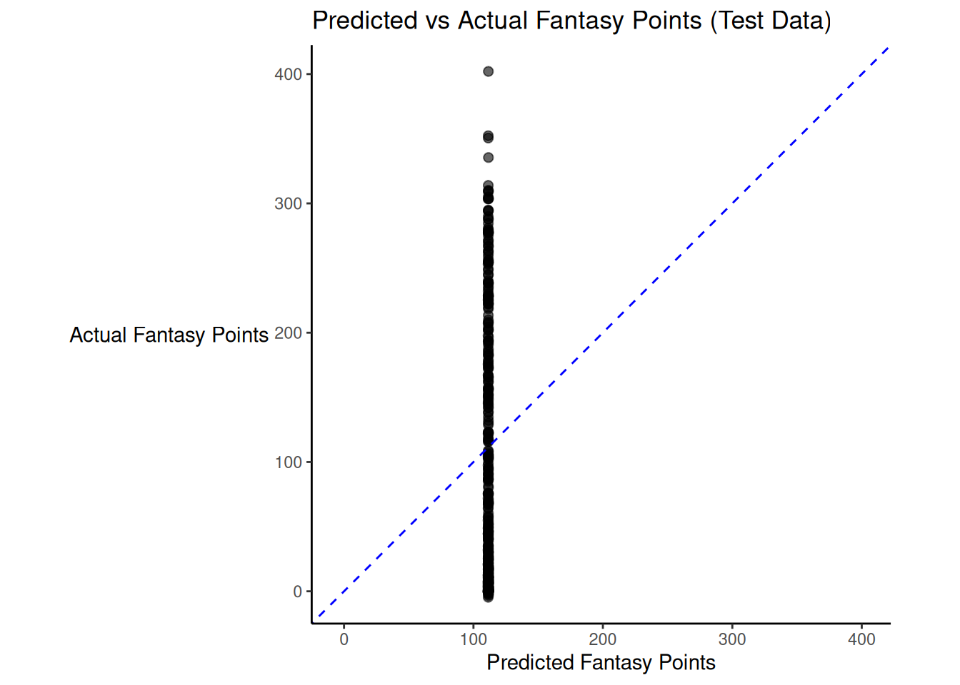
Below are the model predictions for next year’s fantasy points:
Below, we fit a linear regression model with multiple predictors and evaluate it with cross-validation. We also evaluate its accuracy on the hold-out (test) data.
# Set seed for reproducibility
set.seed(52242)
# Set up Cross-Validation
folds <- folds_kFold
# Define Recipe (Formula)
rec <- recipes::recipe(
fantasyPoints_lag ~ ., # use all predictors
data = data_train_qb %>% select(-gsis_id, -fantasyPointsMC_lag))
# Define Model
lm_spec <- parsnip::linear_reg() %>%
parsnip::set_engine("lm") %>%
parsnip::set_mode("regression")
# Workflow
lm_wf <- workflows::workflow() %>%
workflows::add_recipe(rec) %>%
workflows::add_model(lm_spec)
# Fit Model with Cross-Validation
cv_results <- tune::fit_resamples(
lm_wf,
resamples = folds,
metrics = yardstick::metric_set(rmse, mae, rsq),
control = tune::control_resamples(save_pred = TRUE)
)
# View Cross-Validation metrics
tune::collect_metrics(cv_results)There was modest shrinkage from the training model to the test model: the \(R^2\) for the model on the training data was 0.42; the \(R^2\) for the same model applied to the test data was 0.42.
Figure 19.2 depicts the predicted versus actual fantasy points for the model on the test data.
# Calculate combined range for axes
axis_limits <- range(c(df$pred, df$fantasyPoints_lag), na.rm = TRUE)
ggplot(
df,
aes(
x = pred,
y = fantasyPoints_lag)) +
geom_point(
size = 2,
alpha = 0.6) +
geom_abline(
slope = 1,
intercept = 0,
color = "blue",
linetype = "dashed") +
coord_equal(
xlim = axis_limits,
ylim = axis_limits) +
labs(
title = "Predicted vs Actual Fantasy Points (Test Data)",
x = "Predicted Fantasy Points",
y = "Actual Fantasy Points"
) +
theme_classic() +
theme(axis.title.y = element_text(angle = 0, vjust = 0.5)) # horizontal y-axis title
Below are the model predictions for next year’s fantasy points:
Below, we fit a LASSO model. We evaluate it and tune its penalty parameter with cross-validation. The penalty parameter in a LASSO model controls the strength of regularization applied to the model coefficients. Smaller penalty values result in less regularization, allowing the model to retain more predictors with larger (nonzero) coefficients. This typically reduces bias but increases variance of the model’s predictions, as the model may overfit to the training data by including irrelevant or weak predictors. Larger penalty values apply stronger regularization, shrinking more coefficients exactly to zero. This encourages a sparser model that may increase bias (by excluding useful predictors) but reduces variance and improves generalizability by simplifying the model and reducing overfitting.
After tuning the model, we evaluate its accuracy on the hold-out (test) data.
The LASSO models were fit using the glmnet package (Friedman et al., 2010, 2025; Tay et al., 2023).
For the machine learning models, we perform the parameter tuning using the tune::tune(), tune::tune_grid(), tune::select_best(), and tune::finalize_workflow() functions of the tune package (Kuhn, 2025). We specify the grid of possible parameter values using the dials::grid_regular() function of the dials package (Kuhn & Frick, 2025).
# Set seed for reproducibility
set.seed(52242)
# Set up Cross-Validation
folds <- folds_kFold
# Define Recipe (Formula)
rec <- recipes::recipe(
fantasyPoints_lag ~ ., # use all predictors
data = data_train_qb %>% select(-gsis_id, -fantasyPointsMC_lag))
# Define Model
lasso_spec <-
parsnip::linear_reg(
penalty = tune::tune(),
mixture = 1) %>%
parsnip::set_engine("glmnet")
# Workflow
lasso_wf <- workflows::workflow() %>%
workflows::add_recipe(rec) %>%
workflows::add_model(lasso_spec)
# Define grid of penalties to try (log scale is typical)
penalty_grid <- dials::grid_regular(
dials::penalty(range = c(-4, -1)),
levels = 20)
# Tune the Penalty Parameter
cv_results <- tune::tune_grid(
lasso_wf,
resamples = folds,
grid = penalty_grid,
metrics = yardstick::metric_set(rmse, mae, rsq),
control = tune::control_grid(save_pred = TRUE)
)
# View Cross-Validation metrics
tune::collect_metrics(cv_results)best_penalty <- tune::select_best(cv_results, metric = "mae")
# Finalize Workflow with Best Penalty
final_wf <- tune::finalize_workflow(
lasso_wf,
best_penalty)
# Fit Final Model on Training Data
final_model <- workflows::fit(
final_wf,
data = data_train_qb)
# View Coefficients
final_model %>%
workflows::extract_fit_parsnip() %>%
broom::tidy()There was modest shrinkage from the training model to the test model: the \(R^2\) for the model on the training data was 0.43; the \(R^2\) for the same model applied to the test data was 0.44.
Figure 19.3 depicts the predicted versus actual fantasy points for the model on the test data.
# Calculate combined range for axes
axis_limits <- range(c(df$pred, df$fantasyPoints_lag), na.rm = TRUE)
ggplot(
df,
aes(
x = pred,
y = fantasyPoints_lag)) +
geom_point(
size = 2,
alpha = 0.6) +
geom_abline(
slope = 1,
intercept = 0,
color = "blue",
linetype = "dashed") +
coord_equal(
xlim = axis_limits,
ylim = axis_limits) +
labs(
title = "Predicted vs Actual Fantasy Points (Test Data)",
x = "Predicted Fantasy Points",
y = "Actual Fantasy Points"
) +
theme_classic() +
theme(axis.title.y = element_text(angle = 0, vjust = 0.5)) # horizontal y-axis title
Below are the model predictions for next year’s fantasy points:
Below, we fit a ridge regression model. We evaluate it and tune its penalty parameter with cross-validation. The penalty parameter in a ridge regression model controls the amount of regularization applied to the model’s coefficients. Smaller penalty values allow coefficients to remain large, resulting in a model that closely fits the training data. This may reduce bias but increases the risk of overfitting, especially in the presence of multicollinearity or many weak predictors. Larger penalty values shrink coefficients toward zero (though not exactly to zero), which reduces model complexity. This typically increases bias slightly but reduces variance of the model’s predictions, making the model more stable and better suited for generalization to new data.
After tuning the model, we also evaluate its accuracy on the hold-out (test) data.
The ridge regression models were fit using the glmnet package (Friedman et al., 2010, 2025; Tay et al., 2023).
# Set seed for reproducibility
set.seed(52242)
# Set up Cross-Validation
folds <- folds_kFold
# Define Recipe (Formula)
rec <- recipes::recipe(
fantasyPoints_lag ~ ., # use all predictors
data = data_train_qb %>% select(-gsis_id, -fantasyPointsMC_lag))
# Define Model
ridge_spec <-
parsnip::linear_reg(
penalty = tune::tune(),
mixture = 0) %>%
parsnip::set_engine("glmnet")
# Workflow
ridge_wf <- workflows::workflow() %>%
workflows::add_recipe(rec) %>%
workflows::add_model(ridge_spec)
# Define grid of penalties to try (log scale is typical)
penalty_grid <- dials::grid_regular(
dials::penalty(range = c(-4, -1)),
levels = 20)
# Tune the Penalty Parameter
cv_results <- tune::tune_grid(
ridge_wf,
resamples = folds,
grid = penalty_grid,
metrics = yardstick::metric_set(rmse, mae, rsq),
control = tune::control_grid(save_pred = TRUE)
)
# View Cross-Validation metrics
tune::collect_metrics(cv_results)best_penalty <- tune::select_best(cv_results, metric = "mae")
# Finalize Workflow with Best Penalty
final_wf <- tune::finalize_workflow(
ridge_wf,
best_penalty)
# Fit Final Model on Training Data
final_model <- workflows::fit(
final_wf,
data = data_train_qb)
# View Coefficients
final_model %>%
workflows::extract_fit_parsnip() %>%
broom::tidy()There was modest shrinkage from the training model to the test model: the \(R^2\) for the model on the training data was 0.44; the \(R^2\) for the same model applied to the test data was 0.44.
Figure 19.4 depicts the predicted versus actual fantasy points for the model on the test data.
# Calculate combined range for axes
axis_limits <- range(c(df$pred, df$fantasyPoints_lag), na.rm = TRUE)
ggplot(
df,
aes(
x = pred,
y = fantasyPoints_lag)) +
geom_point(
size = 2,
alpha = 0.6) +
geom_abline(
slope = 1,
intercept = 0,
color = "blue",
linetype = "dashed") +
coord_equal(
xlim = axis_limits,
ylim = axis_limits) +
labs(
title = "Predicted vs Actual Fantasy Points (Test Data)",
x = "Predicted Fantasy Points",
y = "Actual Fantasy Points"
) +
theme_classic() +
theme(axis.title.y = element_text(angle = 0, vjust = 0.5)) # horizontal y-axis title
Below are the model predictions for next year’s fantasy points:
Below, we fit an elastic net model. We evaluate it and tune its penalty and mixture parameters with cross-validation.
The penalty parameter controls the overall strength of regularization applied to the model’s coefficients. Smaller penalty values allow coefficients to remain large, which can reduce bias but increase variance of the model’s predictions and can increase the risk of overfitting. Larger penalty values shrink coefficients more aggressively, leading to simpler models with potentially higher bias but lower variance of predictions. This regularization helps prevent overfitting, especially when the model includes many predictors or multicollinearity.
The mixture parameter controls the balance between LASSO and ridge regularization. It ranges from 0 to 1: A value of 0 applies pure ridge regression, which shrinks all coefficients but keeps them in the model. A value of 1 applies pure LASSO, which can shrink some coefficients exactly to zero, effectively performing variable selection. Values between 0 and 1 apply a combination: ridge-like smoothing and LASSO-like sparsity. Smaller mixture values favor shrinkage without variable elimination, whereas larger values favor sparser solutions by excluding weak predictors.
After tuning the model, we also evaluate its accuracy on the hold-out (test) data.
The elastic net models were fit using the glmnet package (Friedman et al., 2010, 2025; Tay et al., 2023).
# Set seed for reproducibility
set.seed(52242)
# Set up Cross-Validation
folds <- folds_kFold
# Define Recipe (Formula)
rec <- recipes::recipe(
fantasyPoints_lag ~ ., # use all predictors
data = data_train_qb %>% select(-gsis_id, -fantasyPointsMC_lag))
# Define Model
enet_spec <-
parsnip::linear_reg(
penalty = tune::tune(),
mixture = tune::tune()) %>%
parsnip::set_engine("glmnet")
# Workflow
enet_wf <- workflows::workflow() %>%
workflows::add_recipe(rec) %>%
workflows::add_model(enet_spec)
# Define a regular grid for both penalty and mixture
grid_enet <- dials::grid_regular(
dials::penalty(range = c(-4, -1)),
dials::mixture(range = c(0, 1)),
levels = c(20, 5) # 20 penalty values × 5 mixture values
)
# Tune the Grid
cv_results <- tune::tune_grid(
enet_wf,
resamples = folds,
grid = grid_enet,
metrics = yardstick::metric_set(rmse, mae, rsq),
control = tune::control_grid(save_pred = TRUE)
)
# View Cross-Validation metrics
tune::collect_metrics(cv_results)best_penalty <- tune::select_best(cv_results, metric = "mae")
# Finalize Workflow with Best Penalty
final_wf <- tune::finalize_workflow(
enet_wf,
best_penalty)
# Fit Final Model on Training Data
final_model <- workflows::fit(
final_wf,
data = data_train_qb)
# View Coefficients
final_model %>%
workflows::extract_fit_parsnip() %>%
broom::tidy()There was modest shrinkage from the training model to the test model: the \(R^2\) for the model on the training data was 0.44; the \(R^2\) for the same model applied to the test data was 0.44.
Figure 19.5 depicts the predicted versus actual fantasy points for the model on the test data.
# Calculate combined range for axes
axis_limits <- range(c(df$pred, df$fantasyPoints_lag), na.rm = TRUE)
ggplot(
df,
aes(
x = pred,
y = fantasyPoints_lag)) +
geom_point(
size = 2,
alpha = 0.6) +
geom_abline(
slope = 1,
intercept = 0,
color = "blue",
linetype = "dashed") +
coord_equal(
xlim = axis_limits,
ylim = axis_limits) +
labs(
title = "Predicted vs Actual Fantasy Points (Test Data)",
x = "Predicted Fantasy Points",
y = "Actual Fantasy Points"
) +
theme_classic() +
theme(axis.title.y = element_text(angle = 0, vjust = 0.5)) # horizontal y-axis title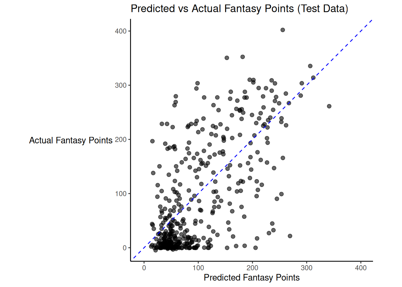
Below are the model predictions for next year’s fantasy points:
A random forest model combines the results of many decision trees. A decision tree splits the data into groups based on the values of the predictors, and then predicts the outcome within each group. A given decision tree can be noisy and prone to overfitting, so random forests build many trees, where each tree is trained on a random subset of the data and considers a random subset of predictors at each split. The random forest then averages the predictions of all the decision trees, to improve overall predictive accuracy.
Below, we fit a random forest model. We evaluate it and tune two parameters with cross-validation. The first parameter is mtry, which controls the number of predictors randomly sampled at each split in a decision tree. Smaller mtry values increase tree diversity by forcing trees to consider different subsets of predictors. This typically reduces the variance of the overall model’s predictions (because the final prediction is averaged over more diverse trees) but may increase bias if strong predictors are frequently excluded. Larger mtry allow more predictors to be considered at each split, making trees more similar to each other. This can reduce bias but often increases variance of the model’s predictions, because the trees are more correlated and less effective at error cancellation when averaged.
The second parameter is min_n, which controls the minimum number of observations that must be present in a node for a split to be attempted. Smaller min_n values allow trees to grow deeper and capture more fine-grained patterns in the training data. This typically reduces bias but increases variance of the overall model’s predictions, because deeper trees are more likely to overfit to noise in the training data. Larger min_n values restrict the depth of the trees by requiring more data to justify a split. This can reduce variance by producing simpler, more generalizable trees—but may increase bias if the trees are unable to capture important structure in the data.
After tuning the model, we evaluate its accuracy on the hold-out (test) data.
The random forest models were fit using the ranger package (Wright, 2024; Wright & Ziegler, 2017). We specify the grid of possible parameter values using the dials::grid_random(), dials::update.parameters(), dials::mtry(), and dials::min_n() functions of the dials package (Kuhn & Frick, 2025) and the hardhat::extract_parameter_set_dials() function of the hardhat package (Frick, Vaughan, et al., 2025).
# Set seed for reproducibility
set.seed(52242)
# Set up Cross-Validation
folds <- folds_kFold
# Define Recipe (Formula)
rec <- recipes::recipe(
fantasyPoints_lag ~ ., # use all predictors
data = data_train_qb %>% select(-gsis_id, -fantasyPointsMC_lag))
# Define Model
rf_spec <-
parsnip::rand_forest(
mtry = tune::tune(),
min_n = tune::tune(),
trees = 500) %>%
parsnip::set_mode("regression") %>%
parsnip::set_engine(
"ranger",
importance = "impurity")
# Workflow
rf_wf <- workflows::workflow() %>%
workflows::add_recipe(rec) %>%
workflows::add_model(rf_spec)
# Create Grid
n_predictors <- recipes::prep(rec) %>%
recipes::juice() %>%
dplyr::select(-fantasyPoints_lag) %>%
ncol()
# Dynamically define ranges based on data
rf_params <- hardhat::extract_parameter_set_dials(rf_spec) %>%
dials:::update.parameters(
mtry = dials::mtry(range = c(1L, n_predictors)),
min_n = dials::min_n(range = c(2L, 10L))
)
rf_grid <- dials::grid_random(rf_params, size = 15) #dials::grid_regular(rf_params, levels = 5)
# Tune the Grid
cv_results <- tune::tune_grid(
rf_wf,
resamples = folds,
grid = rf_grid,
metrics = yardstick::metric_set(rmse, mae, rsq),
control = tune::control_grid(save_pred = TRUE)
)
# View Cross-Validation metrics
tune::collect_metrics(cv_results)best_penalty <- tune::select_best(cv_results, metric = "mae")
# Finalize Workflow with Best Penalty
final_wf <- tune::finalize_workflow(
rf_wf,
best_penalty)
# Fit Final Model on Training Data
final_model <- workflows::fit(
final_wf,
data = data_train_qb)
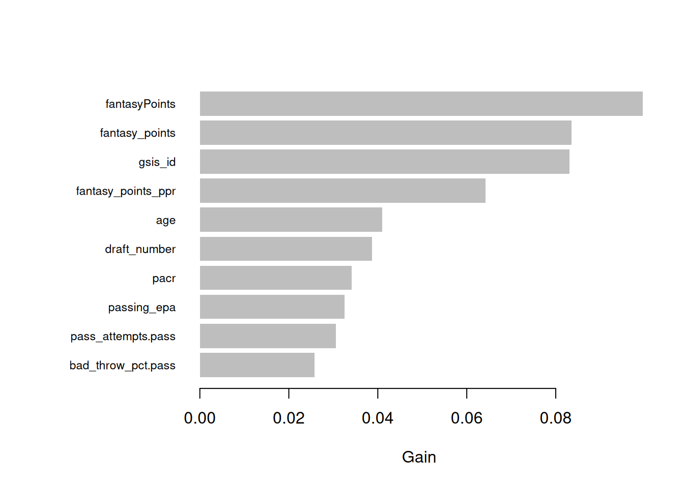
# View Feature Importance
rf_fit <- final_model %>%
workflows::extract_fit_parsnip()
rf_fitparsnip model object
Ranger result
Call:
ranger::ranger(x = maybe_data_frame(x), y = y, mtry = min_cols(~8L, x), num.trees = ~500, min.node.size = min_rows(~6L, x), importance = ~"impurity", num.threads = 1, verbose = FALSE, seed = sample.int(10^5, 1))
Type: Regression
Number of trees: 500
Sample size: 1657
Number of independent variables: 82
Mtry: 8
Target node size: 6
Variable importance mode: impurity
Splitrule: variance
OOB prediction error (MSE): 6563.994
R squared (OOB): 0.4969903 season
133420.73
games
469448.28
gs
562484.63
years_of_experience
127006.89
age
252334.83
ageCentered20
258561.02
ageCentered20Quadratic
267763.35
height
101258.98
weight
170959.45
rookie_season
153420.28
draft_pick
242706.92
fantasy_points
1328938.53
fantasy_points_ppr
1259648.96
fantasyPoints
1286991.50
completions
570249.66
attempts
631443.24
passing_yards
845893.94
passing_tds
981935.01
passing_interceptions
138726.01
sacks_suffered
198722.15
sack_yards_lost
266232.97
sack_fumbles
74314.00
sack_fumbles_lost
48845.36
passing_air_yards
248364.49
passing_yards_after_catch
365702.79
passing_first_downs
781172.41
passing_epa
491894.47
passing_cpoe
203734.37
passing_2pt_conversions
35831.08
pacr
144209.23
carries
236799.97
rushing_yards
158787.03
rushing_tds
56831.77
rushing_fumbles
64977.19
rushing_fumbles_lost
35372.51
rushing_first_downs
183688.40
rushing_epa
197253.22
rushing_2pt_conversions
20299.97
special_teams_tds
0.00
pocket_time.pass
128988.79
pass_attempts.pass
551956.69
throwaways.pass
164802.84
spikes.pass
57550.91
drops.pass
277704.34
bad_throws.pass
419170.14
times_blitzed.pass
457698.12
times_hurried.pass
493238.30
times_hit.pass
213059.90
times_pressured.pass
288785.57
batted_balls.pass
83941.28
on_tgt_throws.pass
341399.06
rpo_plays.pass
128028.20
rpo_yards.pass
162548.15
rpo_pass_att.pass
122303.48
rpo_pass_yards.pass
132341.68
rpo_rush_att.pass
75057.02
rpo_rush_yards.pass
122328.10
pa_pass_att.pass
168849.76
pa_pass_yards.pass
197166.86
intended_air_yards.pass
49572.48
intended_air_yards_per_pass_attempt.pass
42638.20
completed_air_yards.pass
43950.32
completed_air_yards_per_completion.pass
39592.82
completed_air_yards_per_pass_attempt.pass
40437.99
pass_yards_after_catch.pass
41811.58
pass_yards_after_catch_per_completion.pass
30085.88
scrambles.pass
28500.85
scramble_yards_per_attempt.pass
37783.34
drop_pct.pass
165079.16
bad_throw_pct.pass
173515.25
on_tgt_pct.pass
162168.42
pressure_pct.pass
173649.63
ybc_att.rush
175959.76
yac_att.rush
135603.88
att.rush
318384.69
yds.rush
165083.69
td.rush
69837.34
x1d.rush
146133.59
ybc.rush
189402.36
yac.rush
135490.46
brk_tkl.rush
46572.78
att_br.rush
66632.24 There was modest shrinkage from the training model to the test model: the \(R^2\) for the model on the training data was 0.44; the \(R^2\) for the same model applied to the test data was 0.48.
Figure 19.6 depicts the predicted versus actual fantasy points for the model on the test data.
# Calculate combined range for axes
axis_limits <- range(c(df$pred, df$fantasyPoints_lag), na.rm = TRUE)
ggplot(
df,
aes(
x = pred,
y = fantasyPoints_lag)) +
geom_point(
size = 2,
alpha = 0.6) +
geom_abline(
slope = 1,
intercept = 0,
color = "blue",
linetype = "dashed") +
coord_equal(
xlim = axis_limits,
ylim = axis_limits) +
labs(
title = "Predicted vs Actual Fantasy Points (Test Data)",
x = "Predicted Fantasy Points",
y = "Actual Fantasy Points"
) +
theme_classic() +
theme(axis.title.y = element_text(angle = 0, vjust = 0.5)) # horizontal y-axis title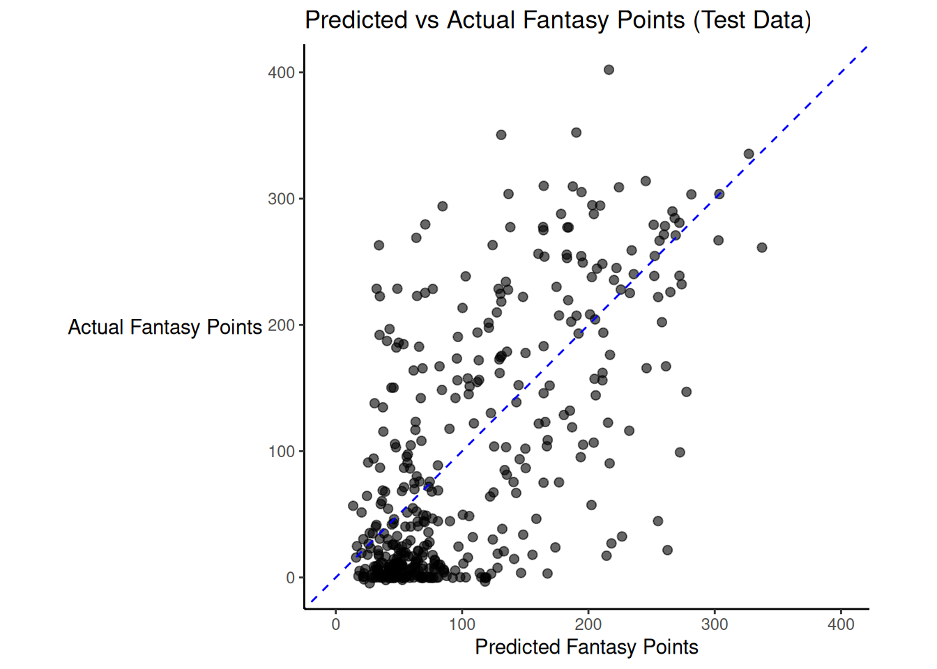
Below are the model predictions for next year’s fantasy points:
Now we can stop the parallel backend:
The above approaches to machine learning assume that the observations are independent across rows. However, in our case, this assumption does not hold because the data are longitudinal—each player has multiple seasons, and each row corresponds to a unique player–season combination. In the approaches below, using a random forest model (this section) and a gradient tree boosting model (in Section 19.8.5), we address this by explicitly accounting for the nesting of longitudinal observations within players.
Approaches to estimating random forest models with longitudinal data are described by Hu & Szymczak (2023). Below, we fit longitudinal random forest models using the LongituRF::MERF() function of the LongituRF package (Capitaine, 2020).
smerf <- LongituRF::MERF(
X = data_train_qb %>% dplyr::select(season:att_br.rush) %>% as.matrix(), # predictors of the fixed effects
Y = data_train_qb[,c("fantasyPoints_lag")] %>% as.matrix(), # outcome variable
Z = data_train_qb %>% dplyr::mutate(constant = 1) %>% dplyr::select(constant, passing_yards, passing_tds, passing_interceptions, passing_epa, pacr) %>% as.matrix(), # predictors of the random effects
id = data_train_qb[,c("gsis_id")] %>% as.matrix(), # player ID (for nesting)
time = data_train_qb[,c("ageCentered20")] %>% as.matrix(), # time variable
ntree = 500,
sto = "BM")Error in `loadNamespace()`:
! there is no package called 'LongituRF'Error:
! object 'smerf' not foundError:
! object 'smerf' not foundError:
! object 'smerf' not foundError:
! object 'smerf' not foundThe following code generates an error, for some reason. This issue has been posted on the GitHub repository: https://github.com/sistm/LongituRF/issues/5. Hopefully the package maintainer will help address the issue.
# Predict on Test Data
predict(
smerf,
X = data_test_qb %>% dplyr::select(season:att_br.rush) %>% as.matrix(),
Z = data_train_qb %>% dplyr::mutate(constant = 1) %>% dplyr::select(constant, passing_yards, passing_tds, passing_interceptions, passing_epa, pacr) %>% as.matrix(),
id = data_test_qb[,c("gsis_id")] %>% as.matrix(),
time = data_test_qb[,c("ageCentered20")] %>% as.matrix())Error:
! object 'smerf' not foundTo combine gradient tree boosting with mixed models, we use the gpboost package (Sigrist et al., 2025). Gradient tree boosting is similar to a random forest model. Gradient tree boosting builds trees one by one, each trying to correct the errors of the previous trees. By contrast, in a random forest model, all trees are built independently and then averaged. This gradient tree boosting approach includes a mixed model to account for the longitudinal data nested within players.
Adapted from here: https://towardsdatascience.com/mixed-effects-machine-learning-for-longitudinal-panel-data-with-gpboost-part-iii-523bb38effc
If using a gamma distribution, it requires positive-only values:
For identifying the optimal tuning parameters for boosting, we partition the training data into inner training data and validation data. We randomly split the training data into 80% inner training data and 20% held-out validation data. We then use the mean absolute error as our index of prediction accuracy on the held-out validation data. We use the gpboost::gpb.Dataset() function to specify the data, the gpboost::GPModel() function to specify the model, and the gpboost::gpb.grid.search.tune.parameters() function to identify the optimal tuning parameters for that model.
# Partition training data into inner training data and validation data
ntrain_qb <- dim(data_train_qb_matrix)[1]
set.seed(52242)
valid_tune_idx_qb <- sample.int(ntrain_qb, as.integer(0.2*ntrain_qb)) # validation set
folds_qb <- list(valid_tune_idx_qb)
# Specify parameter grid, gp_model, and gpb.Dataset
param_grid_qb <- list(
"learning_rate" = c(0.2, 0.1, 0.05, 0.01), # the step size used when updating predictions after each boosting round (high values make big updates, which can speed up learning but risk overshooting; low values are usually more accurate but require more rounds)
"max_depth" = c(3, 5, 7), # maximum depth (levels) of each decision tree; deeper trees capture more complex patterns and interactions but risk overfitting; shallower trees tend to generalize better
"min_data_in_leaf" = c(10, 50, 100), # minimum number of training examples in a leaf node; higher values = more regularization (simpler trees)
"lambda_l2" = c(0, 1, 5)) # L2 regularization penalty for large weights in tree splits; adds a "cost" for complexity; helps prevent overfitting by shrinking the contribution of each tree
other_params_qb <- list(
num_leaves = 2^6) # maximum number of leaves per tree; controls the maximum complexity of each tree (along with max_depth); more leaves = more expressive models, but can overfit if min_data_in_leaf is too small; num_leaves must be consistent with max_depth, because deeper trees naturally support more leaves; max is: 2^n, where n is the largest max_depth
gp_model_qb <- gpboost::GPModel(
group_data = data_train_qb_matrix[,"gsis_id"],
likelihood = model_likelihood,
group_rand_coef_data = cbind(
data_train_qb_matrix[,"ageCentered20"],
data_train_qb_matrix[,"ageCentered20Quadratic"]),
ind_effect_group_rand_coef = c(1,1))
gp_data_qb <- gpboost::gpb.Dataset(
data = data_train_qb_matrix[,pred_vars_qb],
categorical_feature = pred_vars_qb_categorical,
label = data_train_qb_matrix[,"fantasyPoints_lag"]) # could instead use mean-centered variable (fantasyPointsMC_lag) and add mean back afterward
# Find optimal tuning parameters
opt_params_qb <- gpboost::gpb.grid.search.tune.parameters(
param_grid = param_grid_qb,
params = other_params_qb,
num_try_random = NULL,
folds = folds_qb,
data = gp_data_qb,
gp_model = gp_model_qb,
nrounds = nrounds,
early_stopping_rounds = 50, # stops training early if the model hasn’t improved on the validation set in 50 rounds; prevents overfitting and saves time
verbose_eval = 1,
metric = "mae")[GPBoost] [Warning] NaN occured in gradient wrt covariance / auxiliary parameter number 1 (counting starts at 1, total nb. par. = 4). This is replaced with 0
[GPBoost] [Warning] NaN occured in gradient wrt covariance / auxiliary parameter number 2 (counting starts at 1, total nb. par. = 4). This is replaced with 0
[GPBoost] [Warning] NaN occured in gradient wrt covariance / auxiliary parameter number 3 (counting starts at 1, total nb. par. = 4). This is replaced with 0
[GPBoost] [Warning] NaN occured in gradient wrt covariance / auxiliary parameter number 4 (counting starts at 1, total nb. par. = 4). This is replaced with 0 Error in `fd$booster$update()`:
! [GPBoost] [Fatal] NaN occurred in initial approximate negative marginal log-likelihood.Possible solutions: try other initial values ('init_cov_pars') or other tuning parameters in case you apply the GPBoost algorithm (e.g., learning_rate)Error:
! object 'opt_params_qb' not foundWe use the optimal parameters identified during tuning. We use a low learning rate (0.1) to avoid overfitting. We set some light regularization (lambda_l2) for better generalization. We also set the maximum tree depth (max_depth) at 5 to capture complex (up to 5-way) interactions, and set the maximum number of terminal nodes (num_leaves) per tree at \(2^6\) (64)—though the number will not reach greater than \(2^{\text{max depth}} = 2^5 = 32\). We set the minimum number of samples in any leaf (min_data_in_leaf) to be 100.
gp_model_qb <- gpboost::GPModel(
group_data = data_train_qb_matrix[,"gsis_id"],
likelihood = model_likelihood,
group_rand_coef_data = cbind(
data_train_qb_matrix[,"ageCentered20"],
data_train_qb_matrix[,"ageCentered20Quadratic"]),
ind_effect_group_rand_coef = c(1,1))
gp_data_qb <- gpboost::gpb.Dataset(
data = data_train_qb_matrix[,pred_vars_qb],
categorical_feature = pred_vars_qb_categorical,
label = data_train_qb_matrix[,"fantasyPoints_lag"])
params_qb <- list(
learning_rate = 0.1,
max_depth = 5,
min_data_in_leaf = 100,
lambda_l2 = 5,
num_leaves = 2^6,
num_threads = num_cores)
nrounds_qb <- 84 # identify optimal number of trees through iteration and cross-validation
#gp_model_qb$set_optim_params(params = list(optimizer_cov = "nelder_mead")) # to speed up model estimationWe use the gpboost::gpb.train() function to fit the specified model with the specified tuning parameters and dataset.
[GPBoost] [Info] Total Bins 9543
[GPBoost] [Info] Number of data points in the train set: 1657, number of used features: 81
[GPBoost] [Info] [GPBoost with gamma likelihood]: initscore=4.830288
[GPBoost] [Info] Start training from score 4.830288[GPBoost] [Warning] Cannot calculate standard deviations for covariance / auxiliary parameters since the approximated Hessian is not positive definite
[GPBoost] [Warning] Cannot calculate standard deviations for covariance / auxiliary parameters since the approximated Hessian is not positive definite
=====================================================
Model summary:
Nb. observations: 1657
Nb. groups: 331 (Group_1)
Covariance parameters (random effects):
Param. Std. err.
Group_1 0 NaN
Group_1_rand_coef_nb_1 0 NaN
Group_1_rand_coef_nb_2 0 NaN
-----------------------------------------------------
Additional parameters:
Param. Std. err.
shape 0.6054 NaN
=====================================================We evaluate the importance of features using the gpboost::gpb.importance() and gpboost::gpb.plot.importance() functions:
# Model-implied predictions
pred_train_qb <- predict(
gp_model_fit_qb,
data = data_train_qb_matrix[, pred_vars_qb],
group_data_pred = data_train_qb_matrix[, "gsis_id"],
group_rand_coef_data_pred = cbind(
data_train_qb_matrix[, "ageCentered20"],
data_train_qb_matrix[, "ageCentered20Quadratic"]),
predict_var = FALSE,
pred_latent = FALSE)
petersenlab::accuracyOverall(
predicted = pred_train_qb[["response_mean"]],
actual = data_train_qb_matrix[, "fantasyPoints_lag"],
dropUndefined = TRUE
)# Test Model on Test Data
pred_test_qb <- predict(
gp_model_fit_qb,
data = data_test_qb_matrix[,pred_vars_qb],
group_data_pred = data_test_qb_matrix[,"gsis_id"],
group_rand_coef_data_pred = cbind(
data_test_qb_matrix[,"ageCentered20"],
data_test_qb_matrix[,"ageCentered20Quadratic"]),
predict_var = FALSE,
pred_latent = FALSE)
y_pred_test_qb <- pred_test_qb[["response_mean"]] # if outcome is mean-centered, add mean(data_train_qb_matrix[,"fantasyPoints_lag"])
predictedVsActual <- data.frame(
predictedPoints = y_pred_test_qb,
actualPoints = data_test_qb_matrix[,"fantasyPoints_lag"]
)
predictedVsActualThere was moderate shrinkage from the training model to the test model: the \(R^2\) for the model on the training data was 0.65; the \(R^2\) for the same model applied to the test data was 0.43.
Figure 19.8 depicts the predicted versus actual fantasy points for the model on the test data.
# Calculate combined range for axes
axis_limits <- range(c(predictedVsActual$predictedPoints, predictedVsActual$actualPoints), na.rm = TRUE)
ggplot(
predictedVsActual,
aes(
x = predictedPoints,
y = actualPoints)) +
geom_point(
size = 2,
alpha = 0.6) +
geom_abline(
slope = 1,
intercept = 0,
color = "blue",
linetype = "dashed") +
coord_equal(
xlim = axis_limits,
ylim = axis_limits) +
labs(
title = "Predicted vs Actual Fantasy Points (Test Data)",
x = "Predicted Fantasy Points",
y = "Actual Fantasy Points"
) +
theme_classic() +
theme(axis.title.y = element_text(angle = 0, vjust = 0.5)) # horizontal y-axis title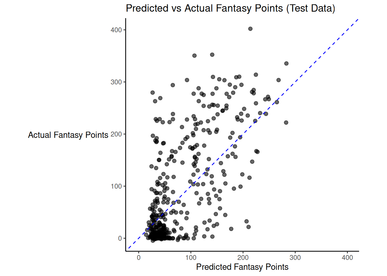
# Generate model predictions for next season
pred_nextYear_qb <- predict(
gp_model_fit_qb,
data = newData_qb_matrix[,pred_vars_qb],
group_data_pred = newData_qb_matrix[,"gsis_id"],
group_rand_coef_data_pred = cbind(
newData_qb_matrix[,"ageCentered20"],
newData_qb_matrix[,"ageCentered20Quadratic"]),
predict_var = FALSE,
pred_latent = FALSE)
newData_qb$fantasyPoints_lag <- pred_nextYear_qb$response_mean
# Merge with player names
newData_qb <- left_join(
newData_qb,
nfl_playerIDs %>% select(gsis_id, name),
by = "gsis_id"
)
newData_qb %>%
arrange(-fantasyPoints_lag) %>%
select(name, fantasyPoints_lag, fantasyPoints)We examined multiple machine learning models that included many predictor variables to identify the model that generates the most accurate prediction of Quarterbacks’ future fantasy points. We also compared them to simpler models, including a regression model with one predictor and a regression model with multiple predictors to determine the incremental validity of the machine learning models above and beyond the simpler models. A summary of the accuracy of the machine learning models is in Table 19.1.
| Model | \(R^2\) | Mean Error | Mean Absolute Error |
|---|---|---|---|
| Regression with One Predictor | 0.45 | 7.42 | 56.99 |
| Regressions with Multiple Predictors | 0.42 | 3.37 | 58.17 |
| LASSO | 0.44 | 3.94 | 57.74 |
| Ridge Regression | 0.44 | 4.36 | 57.60 |
| Elastic Net | 0.44 | 4.36 | 57.60 |
| Random Forest | 0.48 | 9.48 | 55.97 |
| Gradient Tree Boosting | 0.43 | -11.63 | 56.17 |
The most accurate model, in terms of discrimination (\(R^2\)), had an \(R^2\) near 0.48, and it was achieved using a random forest model. The next most accurate model, in terms of discrimination, was a regression model with one predictor: the player’s fantasy points in the previous season. The regression model with one predictor was more accurate (in terms of \(R^2\)) than a regression model with multiple predictors and was just as accurate, if not more accurate, than other machine learning models that leveraged multiple predictors. This suggests that the other predictors examined did not have much incremental validity—they did not show much utility above and beyond a player’s previous fantasy points in predicting their future fantasy points. If anything, considering the additional predictor variables showed decremental validity—the inclusion of the additional variables worsened prediction in several models, possibly by weakening the predictive association of the previous season’s fantasy points and misattributing its predictive effect to other, related predictors in the model. This is consistent with the common finding that simple models (and parsimony) are often preferable. As an example, Youngstrom et al. (2018) found that simple models did just as well and in some cases better than LASSO models in classifying bipolar disorder.
The most accurate model in terms of calibration (mean absolute error) was the random forest model, which had a mean absolute error of 55.97, and was just slightly more accurate than the gradient tree boosting model and the regression model with one predictor. However, even in the most accurate model, the predicted values were over 56 points away from the actual values, suggesting that the model-predicted values were not particularly accurate. In sum, the random forest model, was the most accurate in terms of differentiating between players (\(R^2\)) and was also the most accurate in terms of how close the predicted values were to the actual values.
All models explained less than half of the variance in players’ future fantasy points. Thus, there remains considerable variance to be explained. The considerable unexplained variance suggests that we are missing key variables that are important predictors of future fantasy performance. It is also consistent with the conclusion from many other domains in psychology that human behavior is challenging to predict (Petersen, 2025b). We could likely improve our predictive accuracy by including projections, but it is unclear what information projections are or are not based on. For instance, if projections already account for the prior season’s statistics and fantasy points, then including both may not buy you much in terms of increased predictive accuracy.
Machine learning attempts to maximize prediction accuracy. There are various types of machine learning models. Supervised learning involves learning from data where the correct classification or outcome is known. Unsupervised learning involves learning from data without known classifications. Machine learning can incorporate many predictor variables, so it is important to perform cross-validation to avoid overfitting. We examined multiple machine learning models to identify the model that generates the most accurate prediction of Quarterbacks’ future fantasy points. All models explained less than half of the variance in players’ fantasy points. The most accurate model, in terms of discrimination (\(R^2\)), was achieved using a regression model with one predictor: the player’s fantasy points in the previous season—and a gradient tree boosting model. The most accurate model in terms of calibration (mean absolute error) was the gradient tree boosting model, which accounted for the longitudinal nature of the data. The considerable unexplained variance suggests that we are missing key variables that are important predictors of future fantasy performance.
R version 4.6.1 (2026-06-24)
Platform: x86_64-pc-linux-gnu
Running under: Ubuntu 24.04.4 LTS
Matrix products: default
BLAS: /usr/lib/x86_64-linux-gnu/openblas-pthread/libblas.so.3
LAPACK: /usr/lib/x86_64-linux-gnu/openblas-pthread/libopenblasp-r0.3.26.so; LAPACK version 3.12.0
locale:
[1] LC_CTYPE=C.UTF-8 LC_NUMERIC=C LC_TIME=C.UTF-8
[4] LC_COLLATE=C.UTF-8 LC_MONETARY=C.UTF-8 LC_MESSAGES=C.UTF-8
[7] LC_PAPER=C.UTF-8 LC_NAME=C LC_ADDRESS=C
[10] LC_TELEPHONE=C LC_MEASUREMENT=C.UTF-8 LC_IDENTIFICATION=C
time zone: UTC
tzcode source: system (glibc)
attached base packages:
[1] stats graphics grDevices utils datasets methods base
other attached packages:
[1] glmnet_5.0 Matrix_1.7-5 knitr_1.51 lubridate_1.9.5
[5] forcats_1.0.1 stringr_1.6.0 readr_2.2.0 tibble_3.3.1
[9] tidyverse_2.0.0 effectsize_1.0.3 gpboost_1.7.0 R6_2.6.1
[13] yardstick_1.4.0 workflowsets_1.1.1 workflows_1.3.0 tune_2.1.0
[17] tidyr_1.3.2 tailor_0.1.0 rsample_1.3.2 recipes_1.3.3
[21] purrr_1.2.2 parsnip_1.6.0 modeldata_1.5.1 infer_1.1.0
[25] ggplot2_4.0.3 dplyr_1.2.1 dials_1.4.4 scales_1.4.0
[29] broom_1.0.13 tidymodels_1.5.0 powerjoin_0.1.0 missRanger_2.6.1
[33] future_1.70.0 petersenlab_1.2.3
loaded via a namespace (and not attached):
[1] RColorBrewer_1.1-3 shape_1.4.6.1 rstudioapi_0.19.0
[4] jsonlite_2.0.0 datawizard_1.3.1 magrittr_2.0.5
[7] TH.data_1.1-5 estimability_2.0.0 farver_2.1.2
[10] nloptr_2.2.1 rmarkdown_2.31 vctrs_0.7.3
[13] minqa_1.2.8 base64enc_0.1-6 sparsevctrs_0.3.6
[16] htmltools_0.5.9 Formula_1.2-5 parallelly_1.48.0
[19] htmlwidgets_1.6.4 plyr_1.8.9 sandwich_3.1-2
[22] emmeans_2.0.3 zoo_1.8-15 iterators_1.0.14
[25] lifecycle_1.0.5 pkgconfig_2.0.3 fastmap_1.2.0
[28] rbibutils_2.4.1 digest_0.6.39 colorspace_2.1-3
[31] furrr_0.4.0 Hmisc_5.2-6 labeling_0.4.3
[34] RJSONIO_2.0.5 timechange_0.4.0 compiler_4.6.1
[37] withr_3.0.3 htmlTable_2.5.0 S7_0.2.2
[40] backports_1.5.1 DBI_1.3.0 psych_2.6.5
[43] MASS_7.3-65 lava_1.9.2 tools_4.6.1
[46] pbivnorm_0.6.0 ranger_0.18.0 foreign_0.8-91
[49] otel_0.2.0 future.apply_1.20.2 nnet_7.3-20
[52] glue_1.8.1 quadprog_1.5-8 nlme_3.1-169
[55] grid_4.6.1 checkmate_2.3.4 cluster_2.1.8.2
[58] reshape2_1.4.5 generics_0.1.4 gtable_0.3.6
[61] tzdb_0.5.0 class_7.3-23 hms_1.1.4
[64] data.table_1.18.4 foreach_1.5.2 pillar_1.11.1
[67] mitools_2.4 splines_4.6.1 lattice_0.22-9
[70] FNN_1.1.4.1 survival_3.8-6 tidyselect_1.2.1
[73] mix_1.0-13 reformulas_0.4.4 gridExtra_2.3.1
[76] stats4_4.6.1 xfun_0.60 hardhat_1.4.3
[79] timeDate_4052.112 stringi_1.8.7 DiceDesign_1.10
[82] yaml_2.3.12 boot_1.3-32 evaluate_1.0.5
[85] codetools_0.2-20 cli_3.6.6 rpart_4.1.27
[88] xtable_1.8-8 parameters_0.29.2 Rdpack_2.6.6
[91] lavaan_0.6-21 mirai_2.7.1 Rcpp_1.1.2
[94] globals_0.19.1 coda_0.19-4.1 nanonext_1.10.1
[97] parallel_4.6.1 gower_1.0.2 bayestestR_0.18.1
[100] lme4_2.0-1 listenv_1.0.0 viridisLite_0.4.3
[103] mvtnorm_1.4-2 ipred_0.9-15 prodlim_2026.03.11
[106] insight_1.5.2 rlang_1.3.0 multcomp_1.4-31
[109] mnormt_2.1.2