I want your feedback to make the book better for you and other readers. If you find typos, errors, or places where the text may be improved, please let me know. The best ways to provide feedback are by GitHub or hypothes.is annotations.
You can leave a comment at the bottom of the page/chapter, or open an issue or submit a pull request on GitHub: https://github.com/isaactpetersen/Fantasy-Football-Analytics-Textbook
Alternatively, you can leave an annotation using hypothes.is.
To add an annotation, select some text and then click the
symbol on the pop-up menu.
To see the annotations of others, click the
symbol in the upper right-hand corner of the page.
7 The Fantasy Draft
This chapter provides an overview of the major types of drafts in fantasy football and various draft strategies.
7.1 Getting Started
7.1.1 Load Packages
7.1.2 Load Data
We created the player_stats_weekly.RData and player_stats_seasonal.RData objects in Section 4.4.3. The players_projections_seasonal object was derived from projected points objects that were created in Section 4.3.27.
7.2 Types of Fantasy Drafts
There are several types of drafts in fantasy football. The most common types of drafts are snake drafts and auction drafts.
7.2.1 Snake Draft
In a snake draft, the participants (i.e., managers) are assigned a draft order. In the first round, the managers draft in that order. In the second round, the managers draft in reverse order. It continues to “snake” in this way, round after round, so that the person who has the first pick in a given round has the last pick in the next round, and whoever has the last pick in a given round has the first pick in the next round.
7.2.2 Auction Draft
In an auction draft, the managers are assigned a nomination order and there is a salary cap (e.g., $200). The first manager chooses which player to nominate. Then, the managers bid on that player like in an auction. In order to bid, the manager must raise the price by at least $1. If two managers want to obtain the same player, they may continue to raise the amount until one manager backs out and is no longer to bid by raising the price. The highest bidder wins (i.e., drafts) that player. Then, the second manager nominates a player, and the managers bid on that player. This process repeats until all teams have drafted their allotment of players.
7.2.3 Comparison
Snake drafts are more common than auction drafts. Snake drafts tend to be quicker than auction drafts. However, auction drafts are more fair than snake drafts. In an auction draft, unlike a snake draft, all players are available to all teams. For instance, in a snake draft, the first 9 players drafted are unavailable to the 10th pick of the first round. So, if you have the 10th pick and want the top-ranked player, this player would not be available to you in the snake draft. However, in the auction draft, every player is available to every manager, so long as the manager is able and willing to bid enough.
7.3 Draft Strategy
7.3.1 Overview
There is no one “right” draft strategy. As noted by Lee & Liu (2022) in their analysis of fantasy drafts, the effectiveness of any draft strategy depends on the strategies of the other managers in the league. Sometimes it works best to “zig” when everyone else is “zagging”. For instance, Lee & Liu (2022) found that the most successful draft strategies in terms of roster composition (i.e., the number of players for each position) were not the most common draft strategies. For instance, if you notice that everyone else is drafting Wide Receivers, this may mean that other managers are over-valuing Wide Receivers, and this could be a nice opportunity to draft a Running Back for good value.
In general, you will first want to generate the rankings you will use to select which players to prioritize. You may generate your rankings based one or more of the following:
- your evaluation of players and of their situation
- It may make sense to prioritize players, in particular Running Backs, Wide Receivers, Quarterbacks, and Tight Ends, who are are on strong offenses.
- expert or aggregated rankings
-
layperson rankings
- players’ Average Draft Position (ADP) in other league drafts (for snake drafts)
- players’ Average Auction Value (AAV) in other league drafts (for auction drafts)
- expert or aggregated projections
- indices derived from rankings and projections
As described in Section 26.3, there can be benefits of leveraging the wisdom of the crowd by using rankings or projections that are averaged across many people and perspectives. Section 6.12.1 describes where to obtain aggregated rankings, aggregated projections, ADP, and AAV data. As described in Chapter 15, there are also benefits to using the actuarial approach to prediction rather than (merely) using judgment.
It is not sufficient to compare players in terms of projected points because some positions have more depth than other positions. Some positions show positional scarcity—that is, a limited number of high performing players.
An important concept in the draft is “dropoff”, which is described in Section 6.12.2.1. Dropoff at a given position, is the difference—in terms of projected fantasy points—between (a) the best available player remaining at that position and (b) the second-best available player remaining at that position. If there is a bigger dropoff at a given position, there may be greater value in drafting the top player from that position. For instance, consider the following scenario: “Quarterback A” is projected to score 325 points, and “Quarterback B” is projected to score 320 points. “Tight End A” is projected to score 230 points, and “Tight End B” is projected to score 150 points. In this example, there is a much greater dropoff for Tight Ends than there is for Quarterbacks. Thus, even though “Quarterback A” is projected to score more points than “Tight End A”, “Tight End A” may be more valuable, relatively, because there is still a good Quarterback available if someone else drafts “Quarterback A”. In general, Kickers and Defenses tend to have the lowest dropoff (i.e., the lowest expected drop in fantasy points) by positional rank, so it makes sense to draft Kickers and Defenses late in the draft (Lee & Liu, 2022). Defenses, in particular, appear to be among the least predictable of the positions (Lee & Liu, 2022).
Another important concept is a player’s value over a typical replacement player at that position (shortened to “value over replacement player”; VORP), which is described in Section 6.12.2.2. A player’s value over a typical replacement player provides a way to more fairly compare (and thus rank) players across different positions.
Another important concept is a player’s uncertainty, which is described in Section 6.12.2.3.
In both snake and auction draft formats, your goal is to draft the team whose weekly starting lineup scores the most points and thus the collection of players with the greatest VORP. For your starting lineup, it may make sense—especially with your earliest selections—when comparing two players with equivalent VORP, to prioritize players with higher consistency and lower uncertainty, because they may be considered “safer” with a higher floor. However, when drafting players for your bench, it make make more sense to prioritize high-risk, high reward players with greater uncertainty, because they may have a higher ceiling. Players with a higher ceiling have a potential to be “sleepers”—players who are valued low (i.e., with a high ADP or low AAV) and who outperform their valuation. Note that, although players with greater uncertainty are high-risk, high-reward players, selecting this kind of a player for your bench (i.e., in a late round or for a small cost) is a lower risk selection, because you have less to lose with later/lower-cost picks. That is, even though the player is higher risk, selecting a higher risk player for your bench is a lower risk decision.
The Spurs in the National Basketball Association (NBA) were well-reputed for excelling in this draft strategy (Ryan, 2013; archived at https://perma.cc/X7NW-WZC6). They frequently used their second-round picks to draft high-risk, high-reward players. Sometimes, the secound round pick was a bust, but they have little to lose with a failed second round pick. Other times, their second round picks—including Willie Anderson, DeJuan Blair, Goran Dragic, Luis Scola, and Manu Ginóbili—greatly outperformed expectations. Thanks, in part, to this draft strategy, the team showed strong extended success for nearly three decades from 1989 through the late-2010s.
Another approach is to embrace variability and increase the variability of a team’s outcomes by stacking players from the same team (Lee & Liu, 2022).
However, the draft strategies to achieve the “optimal lineup” differ between snake versus auction drafts.
One factor that is not included above is whether a player is on your favorite team. Managers commonly like to draft players on their favorite teams (e.g., Cowboys, Eagles). That is fine—fantasy football is a game. Do what is fun for you. However, if your goal is to select the best players, leave your allegiances at the door. Selecting players based on their playing for your favorite team—rather than based on performance—is a form of cognitive bias called in-group bias.
In general, the most consequential decisions tend to be those made early in the draft regarding the top projected players (Lee & Liu, 2022). That is, the earlier selections tend to have the greatest impact on the success of one’s fantasy season. So, make sure to spend time in your draft preparation to identify the players you want to select early in the draft. Moreover, some teams like to hedge their bet on their top Running Backs in the case that the player were to get injured, by drafting the player’s backup, a strategy known as handcuffing. However, there is not strong evidence that handcuffing leads to better outcomes (Lee & Liu, 2022).
In general, Lee & Liu (2022) found that teams that drafted more Running Backs and Wide Receivers tended to outperform other teams.
7.3.2 Snake Draft
In general, your goal is to draft the team whose weekly starting lineup has the greatest VORP. Consequently, you are often looking to pick the player with the highest VORP at a given selection, while keeping in mind (a) the dropoff of players at other positions and (b) which players may be available at subsequent picks so that you do not sacrifice too much later value with a given selection. For instance, if a particular Quarterback has a slightly higher VORP than a particular Running Back, but the Quarterback is likely to be available at the manager’s next pick but the Running Back is likely to be unavailable at their next pick, it might make more sense to draft the Running Back. Another way to draft players who are a good value at a given pick is to identify players who have fallen past their ADP (Harstad, 2023; archived at https://perma.cc/9MAC-PUGL). For instance, if you are on pick 30, drafting a player who has fallen past their ADP might mean drafting a player whose ADP is 22.
Herding behavior is common in snake drafts. As described in Section 26.3, herding occurs when people align their behavior with others. For instance, Lee & Liu (2022) found evidence that when Quarterbacks, Kickers, and Defenses were drafted by one team, subsequent teams were more likely to draft a player of that position. The same was not the case for Running Backs, Wide Receivers, and Tight Ends.
Engaging in herding behavior—by following a run, i.e., drafting a player at the same position as previous drafters—can be harmful. For instance, if the run on Quarterbacks is premature, it can lead the “herd” (i.e., the managers who draft a Quarterback after the previous drafters) to spend important draft capital that could have yielded more impactful players at other positions. However, engaging in herding behavior is not always harmful. Herding behavior can be rational if a) there is positional scarcity, or if b) not drafting a player at that position would leave with you without a serviceable option at that position. Position scarcity refers to the dropoff of fantasy points after the top tier of a position—i.e., how steeply player value declines as you move down the rankings, as depicted in Section 7.4.1. For instance, Quarterbacks and Tight Ends tend to show greater positional scarcity than Running Backs and Wide Receivers. That is, there tend to be fewer elite options available at Quarterback and Tight End than at Running Back and Wide Receiver. So, in leagues that have two Quarterbacks on the starting roster or a superflex position (i.e., QB/RB/WR/TE), herding due to positional scarcity can be strategically sound. In general, though, it may be optimal to either a) be at the beginning of a run (i.e., to be the manager who drafts a player, which leads to a run on that position) to secure a scarce, elite option, or b) to avoid the run altogether (by waiting to draft that position later), rather than joining the run in the middle or at the end.
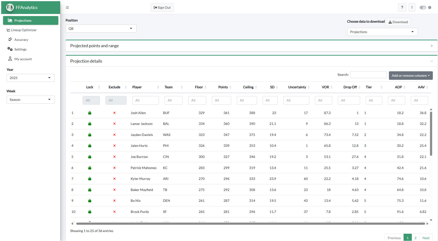
FantasyFootballAnalytics.net provides tools to help you win your snake draft: https://fantasyfootballanalytics.net/win-your-snake-draft. For draft tools for snake drafts, see the Fantasy Football Analytics web application (depicted in Figure 7.1): https://apps.fantasyfootballanalytics.net. The web application includes a free tool that allows users to specify their custom league settings to calculate projected points that are customized to their league and helps users select which players to draft that maximize the players’ value over replacement players (VORP).
7.3.3 Auction Draft
According to an analysis by the Harvard Sports Analysis Collective, the majority of the manager’s salary cap should be spent on the starting lineup, and you should spend less on bench players (Chakravarthy, 2012; archived at https://perma.cc/P7RX-92UU). This is known as the “stars and scrubs” draft strategy. Based on the analysis, the author recommended applying a 10% premium to the top players and a 10% discount to the lower-tiered players. The idea behind the approach is that a player on your bench does not contribute to the team’s points and, thus, most players drafted to your bench do not contribute much to the team’s points throughout the season. That said, bench players can be important in the case of a starter’s injury or under-performance. So, it is recommended to draft starters with lower uncertainty who are safer. In contrast to your starting lineup, you may look to draft players on your bench who have greater uncertainty for their high reward potential in a low-risk selection given the lower price.
An alternative to the “stars and scrubs” approach is to wait to draft more “high-value” players after other managers have over-paid for players. In any case, having some small amount of cap left over toward the end of the draft can help you draft good value players to fill out your bench spots for cheap (e.g., $2). Having some depth can help you offset the impacts of bye weeks, the risk of injuries, and the possibility that some of your starters may underperform their expectation, which is quite likely given how challenging it is to predict fantasy performance.
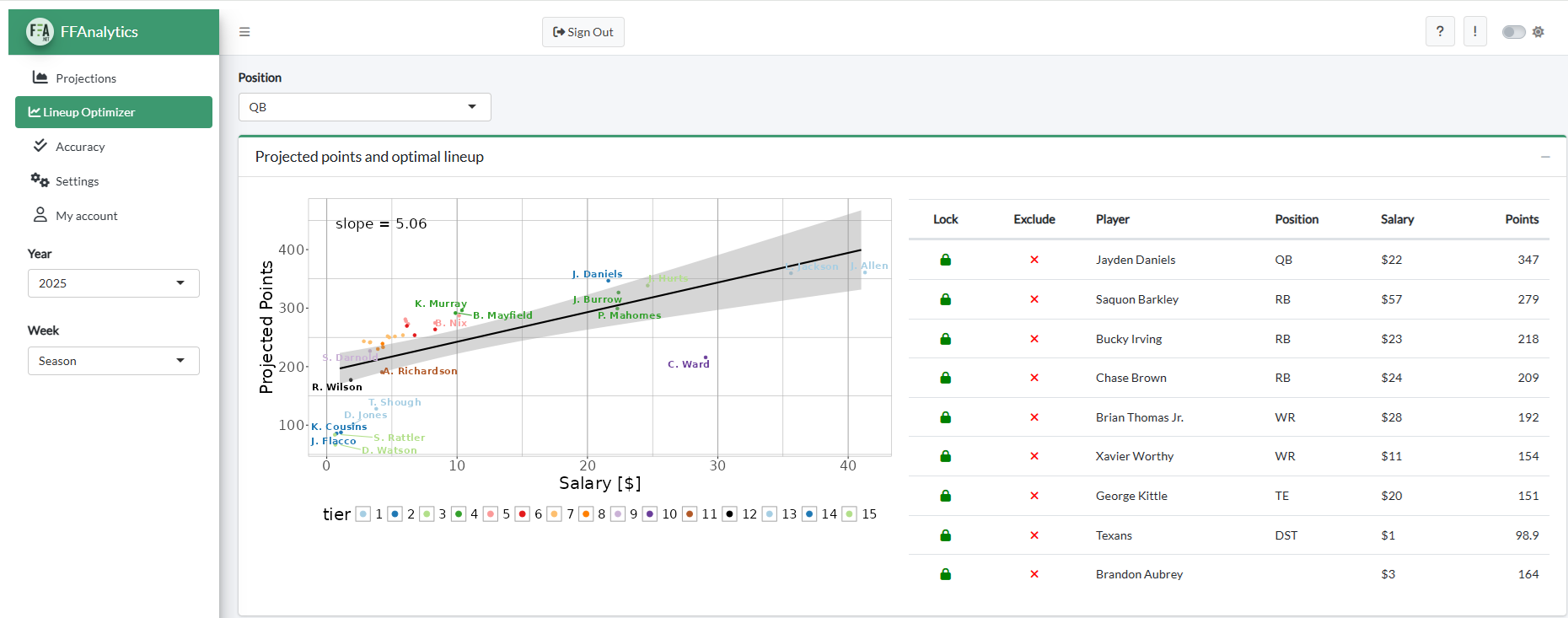
FantasyFootballAnalytics.net provides tools to help you win your auction draft (https://fantasyfootballanalytics.net/how-to-win-your-auction-draft) and daily fantasy sports (DFS) leagues (https://fantasyfootballanalytics.net/how-to/dfsoptimizerhelp). For draft and player selection tools for auction drafts and DFS leagues, see the Fantasy Football Analytics web application (depicted in Figure 7.2): https://apps.fantasyfootballanalytics.net. The web application includes a free tool that allows users to specify their custom league settings to calculate projected points that are customized to their league, and to identify the optimal lineup given their league settings and salary cap.
7.4 Draft Analysis
7.4.1 Fantasy Points by (End-of-Season) Position Rank and Position
A plot of fantasy points by end-of-season position rank and position is depicted in Figure 7.3.
Code
ggplot(
  data = fantasyPointsByPositionRank %>% filter(positionRank <= 200),
  mapping = aes(
    x = positionRank,
    y = fantasyPoints
  )
) +
  geom_point(
    alpha = 0.03
  ) +
  geom_smooth() +
  coord_cartesian(
    ylim = c(0,NA),
    expand = FALSE) + # don't add space between axes and data
  labs(
    x = "End-of-Season Position Rank",
    y = "Fantasy Points (Season)",
    title = "Fantasy Points (Season) by End-of-Season Position Rank"
  ) +
  theme_bw() +
  facet_wrap(vars(position_group)) # facet by position_group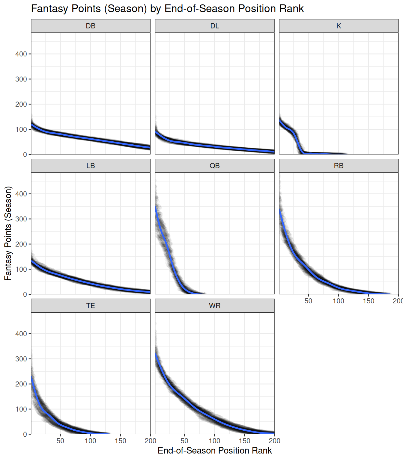
In Figure 7.4, we overlay the smoothed best-fit line for each position onto the same graphing area for direct comparison.
Code
palette_OkabeIto_black <- c("#E69F00", "#56B4E9", "#009E73", "#F0E442", "#0072B2", "#D55E00", "#CC79A7", "#000000")

ggplot(
  data = fantasyPointsByPositionRank %>% filter(positionRank <= 200),
  mapping = aes(
    x = positionRank,
    y = fantasyPoints,
    color = position_group
  )
) +
  geom_smooth(
    linewidth = 1.5,
    se = FALSE) +
  coord_cartesian(
    ylim = c(0,NA), # set limits of y-axis
    expand = FALSE) + # don't add space between axes and data
  scale_color_manual(
    values = palette_OkabeIto_black
  ) +
  labs(
    x = "End-of-Season Position Rank",
    y = "Fantasy Points (Season)",
    title = "Fantasy Points (Season) by End-of-Season Position Rank",
    color = "Position Group"
  ) +
  theme_classic()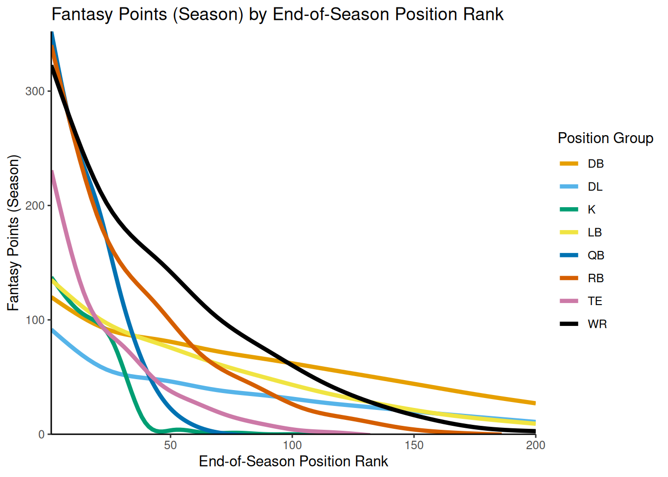
In Figure 7.5, we limit the position rank to ranks less than or equal to 30, for easier comparison of positions’ comparative dropoff at the top position ranks.
Code
ggplot(
  data = fantasyPointsByPositionRank %>% filter(positionRank <= 30),
  mapping = aes(
    x = positionRank,
    y = fantasyPoints,
    color = position_group
  )
) +
  geom_smooth(
    linewidth = 1.5,
    se = FALSE) +
  coord_cartesian(
    ylim = c(0,425), # set limits of y-axis
    expand = FALSE) + # don't add space between axes and data
  scale_color_manual(
    values = palette_OkabeIto_black
  ) +
  labs(
    x = "End-of-Season Position Rank",
    y = "Fantasy Points (Season)",
    title = "Fantasy Points (Season) by End-of-Season Position Rank",
    subtitle = "Position Rank \u2264 30", # \u2264: <= symbol
    color = "Position Group"
  ) +
  theme_classic()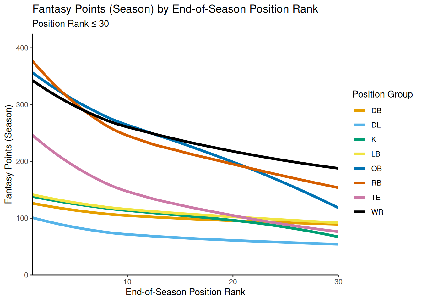
Running Backs show the fastest intial dropoff (i.e., steepest negative slope), followed by Tight Ends, Quarterbacks, Wide Receivers, and then defensive positions. So, identifying the top-scoring Running Back can be of great benefit. After the top 10 or so players at each position, Quarterbacks show a steeper dropoff than Running Backs, Tight Ends, and Wide Receivers.
However, the style of gameplay has changed. Figure 7.6 depicts the same data since 2020.
Code
ggplot(
  data = fantasyPointsByPositionRank %>% filter(positionRank <= 30 & season >= 2020),
  mapping = aes(
    x = positionRank,
    y = fantasyPoints,
    color = position_group
  )
) +
  geom_smooth(
    linewidth = 1.5,
    se = FALSE) +
  coord_cartesian(
    ylim = c(0,425), # set limits of y-axis
    expand = FALSE) + # don't add space between axes and data
  scale_color_manual(
    values = palette_OkabeIto_black
  ) +
  labs(
    x = "End-of-Season Position Rank",
    y = "Fantasy Points (Season)",
    title = "Fantasy Points (Season) by End-of-Season Position Rank",
    subtitle = "Position Rank \u2264 30, Since 2020", # \u2264: <= symbol
    color = "Position Group"
  ) +
  theme_classic()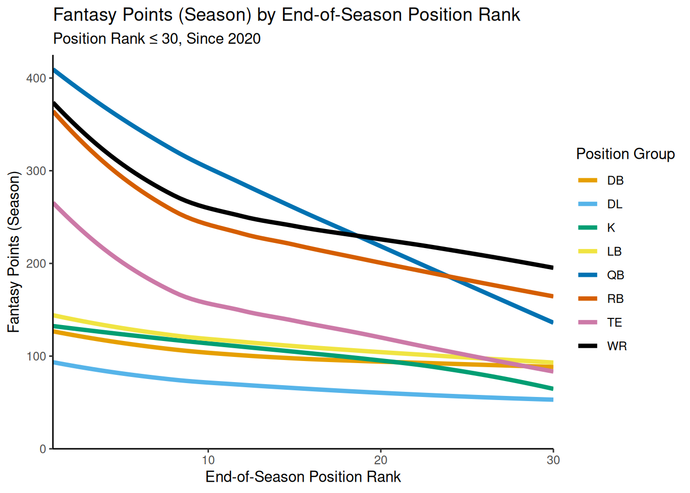
Since 2020, although Running Backs show the fastest initial dropoff, Quarterbacks and Wide Receivers have appeared to overtake them in terms of fantasy points. Quarterbacks continue to show the steepest dropoff after the top 10 or so players at each position.
Figure 7.7 depicts the mean fantasy points of the top 10 players at each position by season.
Code
meanFantasyPointsTop10ByPosition <- fantasyPointsByPositionRank %>%
  filter(positionRank <= 10) %>%
  summarise(
    fantasyPoints = mean(fantasyPoints, na.rm = TRUE),
    .groups = "drop_last"
  )

ggplot(
  data = meanFantasyPointsTop10ByPosition,
  mapping = aes(
    x = season,
    y = fantasyPoints,
    color = position_group
  )
) +
  geom_line(
    linewidth = 1.5) +
  coord_cartesian(
    ylim = c(0,425), # set limits of y-axis
    expand = FALSE) + # don't add space between axes and data
  scale_color_manual(
    values = palette_OkabeIto_black
  ) +
  labs(
    x = "Season",
    y = "Mean Fantasy Points",
    title = "Mean Fantasy Points of Top 10 Players at Each Position by Season",
    color = "Position Group"
  ) +
  theme_classic()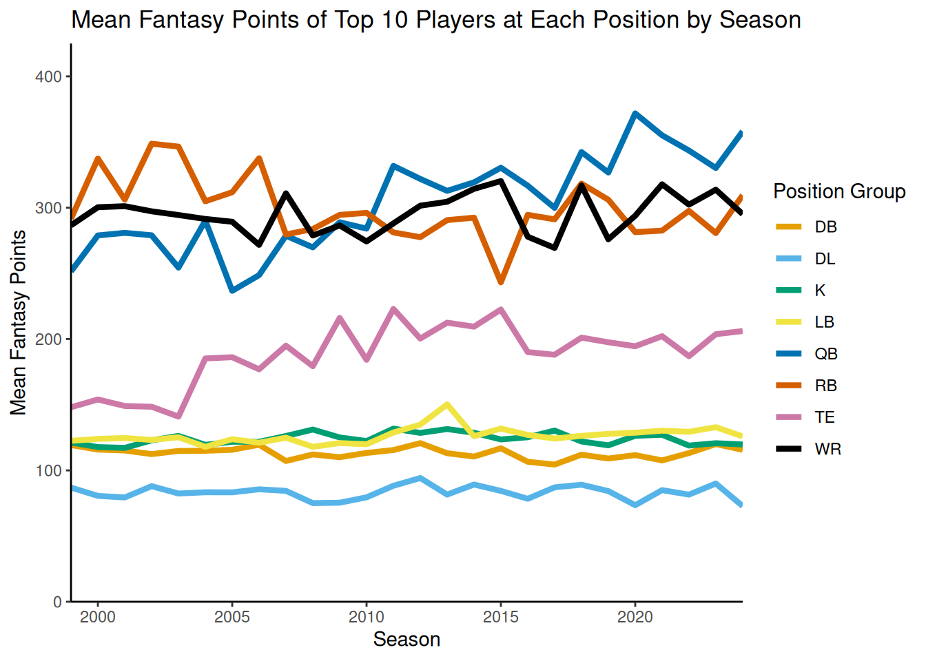
The trend suggests that, since 2000, Quarterbacks have increased in fantasy points scored, and Running Backs have decreased in fantasy points scored.
Key takeaways include that, based on their steep initial dropoff, it can be of great benefit (in terms of a comparative advantage against your opponents) to have a top Running Back or Tight End. The challenge, of course, is identifying—in advance—which of the players is going to be the top-ranked player at that position. It also seems important to have a top-10 Quarterback, because Quarterbacks show the steepest dropoff after position rank of ~10. In general, given their tendency to score lots of points and to show a relatively steep dropoff, it seems crucial to have strong Quarterbacks, Wide Receivers, and Running Backs, with the highest priority likely going to Running Backs and Wide Receivers.
7.4.2 Lineup Optimization
For auction drafts and daily fantasy sports (DFS) leagues, a key goal is to select the best lineup or team within the given cap. For instance, in an auction draft, you may have a $200 cap and your goal is to draft the best team that you can with the $200. Using a mixed-integer programming solver, we can identify the lineup with the most projected points given a particular salary cap. For projected points for a player, we use their average projected points across all available projection sources. For a player’s estimated cost, we use their Average Auction Value (AAV), rounded up to the nearest integer.
We first subset and prepare the data so we can perform the lineup optimization.
Code
mostRecentProjections <- players_projections_seasonal_average_merged %>%
  filter(season == max(season, na.rm = TRUE)) %>%
  filter(pos %in% c("QB","RB","WR","TE","K","DST")) %>%
  filter(avg_type == "average")

# Convert NAs for fantasy points to zero
mostRecentProjections$points[which(is.na(mostRecentProjections$points))] <- 0

# Convert NA for AAV to $1
mostRecentProjections$aav[which(is.na(mostRecentProjections$aav))] <- 1

# Round up AAV to nearest integer
mostRecentProjections$cost <- ceiling(mostRecentProjections$aav)

mostRecentProjections$name <- paste(mostRecentProjections$first_name, mostRecentProjections$last_name)
Next, we set up the constraints. Our example is adapted from https://stackoverflow.com/questions/15147398/optimize-value-with-linear-or-non-linear-constraints-in-r. Our constraints were:
- 9 total players of the following number at each of following positions:
- 1 Quarterback
- 2 Running Backs
- 2 Wide Receivers
- 1 Tight End
- 1 Flex: RB/WR/TE
- 1 K
- 1 DST
- salary cap of $200.
Code
# number of players
num.players <- nrow(mostRecentProjections)

# 1 for every player
total_players <- rep(1, num.players)

# the variables are booleans
var.types <- rep("B", num.players)

# the constraints
A <- rbind(
  as.numeric(mostRecentProjections$pos == "QB"),                # num QB
  as.numeric(mostRecentProjections$pos == "RB"),                # num RB
  as.numeric(mostRecentProjections$pos == "WR"),                # num WR
  as.numeric(mostRecentProjections$pos == "TE"),                # num TE
  as.numeric(mostRecentProjections$pos == "K"),                 # num K
  as.numeric(mostRecentProjections$pos == "DST"),               # num DST
  as.numeric(mostRecentProjections$pos %in% c("RB","WR","TE")), # num flex
  total_players,
  mostRecentProjections$cost)                                   # player cost

dir <- c(
  "==",
  ">=",
  ">=",
  ">=",
  "==",
  "==",
  "==",
  "==",
  "<=")

b <- c(
  1,   # 1 QB
  2,   # at least 2 RBs
  2,   # at least 2 WRs
  1,   # at least 1 TE
  1,   # 1 K
  1,   # 1 DST
  6,   # 1 RB/WR/TE flex (i.e., 6 total RB/WR/TEs)
  9,   # 9 total players
  200) # salary cap of $200
The optimizer thus seeks to identify the lineup with the most projected points that meets the above constraints (within a salary cap of $200). We perform the optimization using the Rglpk::Rglpk_solve_LP() function of the Rglpk package (Theussl & Hornik, 2024).
Here is the solution obtained by the solver:
$optimum
[1] 2272.623

$solution
  [1] 0 0 1 0 0 0 0 0 0 0 0 0 0 0 0 0 0 0 0 0 0 0 0 0 0 0 0 0 0 0 0 0 0 0 0 0 0
 [38] 0 0 0 0 0 0 0 0 0 0 0 0 0 0 0 0 0 0 0 0 0 0 0 0 0 0 0 0 0 0 0 0 0 0 0 0 0
 [75] 0 0 0 0 0 0 0 0 0 0 0 0 0 1 0 0 0 0 0 0 0 1 0 0 0 0 0 0 0 0 0 0 0 0 0 0 0
[112] 0 0 0 0 0 0 0 0 0 0 0 0 0 0 0 0 0 0 0 0 0 0 0 0 0 0 0 0 0 0 0 0 0 0 0 0 0
[149] 0 0 0 0 0 0 0 0 0 0 0 0 0 0 0 0 0 0 0 0 0 0 0 0 0 0 0 0 0 0 0 0 0 0 0 0 0
[186] 0 0 0 0 0 0 0 0 0 0 0 0 0 0 0 0 0 0 0 0 0 0 0 0 0 0 0 0 0 0 0 0 0 0 0 0 0
[223] 0 0 0 0 0 0 0 0 0 0 0 0 0 0 0 0 1 0 0 1 0 0 0 0 0 1 0 0 0 0 0 0 0 0 0 0 0
[260] 0 0 0 0 0 0 0 0 0 0 0 0 0 0 0 0 0 0 0 0 0 0 0 0 0 0 0 0 0 0 0 0 0 0 0 0 0
[297] 0 0 0 0 0 0 0 0 0 0 0 0 0 0 0 0 0 0 0 0 0 0 0 0 0 0 0 0 0 0 0 0 0 0 0 0 0
[334] 0 0 0 0 0 0 0 0 0 0 0 0 0 0 0 0 0 0 0 0 0 0 0 0 0 0 0 0 0 0 0 0 0 0 0 0 0
[371] 0 0 0 0 0 0 0 0 0 0 0 0 0 0 0 0 0 0 0 0 0 0 0 0 0 0 0 0 0 0 0 0 0 0 0 0 0
[408] 0 0 0 0 0 0 0 0 0 0 0 0 0 0 0 0 0 0 0 0 0 0 0 0 0 0 0 0 0 0 0 0 0 0 0 0 0
[445] 0 0 1 0 0 0 0 0 0 0 0 0 0 0 0 0 0 0 0 0 0 0 0 0 0 0 0 0 0 0 0 0 0 0 0 0 0
[482] 0 0 0 0 0 0 0 0 0 0 0 0 0 0 0 0 0 0 0 0 0 0 0 0 0 0 0 0 0 0 0 0 0 0 0 0 0
[519] 0 0 0 0 0 0 0 0 0 0 0 0 0 0 0 0 0 0 0 0 0 0 0 0 0 0 0 0 0 0 0 0 0 0 0 0 0
[556] 0 0 0 0 0 0 0 0 0 0 0 0 0 0 0 0 0 0 0 1 0 0 0 0 0 0 0 0 0 0 0 0 0 0 0 0 0
[593] 0 0 0 0 0 0 0 0 0 0 0 0 0 0 0 0 0 0 0 0 0 0 0 0 0 0 0 1 0 0 0 0 0 0 0 0 0
[630] 0 0 0 0 0 0 0 0 0 0 0 0 0 0 0 0 0 0 0 0 0 0

$status
[1] 0

$solution_dual
[1] NA

$auxiliary
$auxiliary$primal
[1]   1   2   3   1   1   1   6   9 200

$auxiliary$dual
[1] NA


$sensitivity_report
[1] NA
A zero for status indicates that it found a solution:
Here is the maximum value obtained in terms of the sum of projected points for the optimal lineup:
Here is a vector indicating whether or not a given player was selected for the optimal lineup (0 = no; 1 = yes):
  [1] 0 0 1 0 0 0 0 0 0 0 0 0 0 0 0 0 0 0 0 0 0 0 0 0 0 0 0 0 0 0 0 0 0 0 0 0 0
 [38] 0 0 0 0 0 0 0 0 0 0 0 0 0 0 0 0 0 0 0 0 0 0 0 0 0 0 0 0 0 0 0 0 0 0 0 0 0
 [75] 0 0 0 0 0 0 0 0 0 0 0 0 0 1 0 0 0 0 0 0 0 1 0 0 0 0 0 0 0 0 0 0 0 0 0 0 0
[112] 0 0 0 0 0 0 0 0 0 0 0 0 0 0 0 0 0 0 0 0 0 0 0 0 0 0 0 0 0 0 0 0 0 0 0 0 0
[149] 0 0 0 0 0 0 0 0 0 0 0 0 0 0 0 0 0 0 0 0 0 0 0 0 0 0 0 0 0 0 0 0 0 0 0 0 0
[186] 0 0 0 0 0 0 0 0 0 0 0 0 0 0 0 0 0 0 0 0 0 0 0 0 0 0 0 0 0 0 0 0 0 0 0 0 0
[223] 0 0 0 0 0 0 0 0 0 0 0 0 0 0 0 0 1 0 0 1 0 0 0 0 0 1 0 0 0 0 0 0 0 0 0 0 0
[260] 0 0 0 0 0 0 0 0 0 0 0 0 0 0 0 0 0 0 0 0 0 0 0 0 0 0 0 0 0 0 0 0 0 0 0 0 0
[297] 0 0 0 0 0 0 0 0 0 0 0 0 0 0 0 0 0 0 0 0 0 0 0 0 0 0 0 0 0 0 0 0 0 0 0 0 0
[334] 0 0 0 0 0 0 0 0 0 0 0 0 0 0 0 0 0 0 0 0 0 0 0 0 0 0 0 0 0 0 0 0 0 0 0 0 0
[371] 0 0 0 0 0 0 0 0 0 0 0 0 0 0 0 0 0 0 0 0 0 0 0 0 0 0 0 0 0 0 0 0 0 0 0 0 0
[408] 0 0 0 0 0 0 0 0 0 0 0 0 0 0 0 0 0 0 0 0 0 0 0 0 0 0 0 0 0 0 0 0 0 0 0 0 0
[445] 0 0 1 0 0 0 0 0 0 0 0 0 0 0 0 0 0 0 0 0 0 0 0 0 0 0 0 0 0 0 0 0 0 0 0 0 0
[482] 0 0 0 0 0 0 0 0 0 0 0 0 0 0 0 0 0 0 0 0 0 0 0 0 0 0 0 0 0 0 0 0 0 0 0 0 0
[519] 0 0 0 0 0 0 0 0 0 0 0 0 0 0 0 0 0 0 0 0 0 0 0 0 0 0 0 0 0 0 0 0 0 0 0 0 0
[556] 0 0 0 0 0 0 0 0 0 0 0 0 0 0 0 0 0 0 0 1 0 0 0 0 0 0 0 0 0 0 0 0 0 0 0 0 0
[593] 0 0 0 0 0 0 0 0 0 0 0 0 0 0 0 0 0 0 0 0 0 0 0 0 0 0 0 1 0 0 0 0 0 0 0 0 0
[630] 0 0 0 0 0 0 0 0 0 0 0 0 0 0 0 0 0 0 0 0 0 0
Here is the optimal lineup that maximized the sum of projected points within the salary cap:
For a web application that includes a lineup optimizer for selecting the optimal lineup for auction drafts and for DFS leagues, see the Fantasy Football Analytics web application: https://apps.fantasyfootballanalytics.net. The web application allows users to specify their custom league settings, select players to draft or exclude, and exclude risky players, among other features.
7.5 Conclusion
The two major draft types are snake drafts and auction drafts. Auction drafts take longer than snake drafts but are more fair because every player is available to every manager, so long as the manager is able and willing to bid enough. There is no one right draft strategy. In general, it is helpful to draft players with the best value over other players at their position.
7.6 Session Info
R version 4.6.1 (2026-06-24)
Platform: x86_64-pc-linux-gnu
Running under: Ubuntu 24.04.4 LTS

Matrix products: default
BLAS:   /usr/lib/x86_64-linux-gnu/openblas-pthread/libblas.so.3
LAPACK: /usr/lib/x86_64-linux-gnu/openblas-pthread/libopenblasp-r0.3.26.so;  LAPACK version 3.12.0

locale:
 [1] LC_CTYPE=C.UTF-8       LC_NUMERIC=C           LC_TIME=C.UTF-8
 [4] LC_COLLATE=C.UTF-8     LC_MONETARY=C.UTF-8    LC_MESSAGES=C.UTF-8
 [7] LC_PAPER=C.UTF-8       LC_NAME=C              LC_ADDRESS=C
[10] LC_TELEPHONE=C         LC_MEASUREMENT=C.UTF-8 LC_IDENTIFICATION=C

time zone: UTC
tzcode source: system (glibc)

attached base packages:
[1] stats     graphics  grDevices utils     datasets  methods   base

other attached packages:
 [1] Rglpk_0.6-5.1   slam_0.1-55     lubridate_1.9.5 forcats_1.0.1
 [5] stringr_1.6.0   dplyr_1.2.1     purrr_1.2.2     readr_2.2.0
 [9] tidyr_1.3.2     tibble_3.3.1    ggplot2_4.0.3   tidyverse_2.0.0

loaded via a namespace (and not attached):
 [1] Matrix_1.7-5       gtable_0.3.6       jsonlite_2.0.0     compiler_4.6.1
 [5] tidyselect_1.2.1   splines_4.6.1      scales_1.4.0       yaml_2.3.12
 [9] fastmap_1.2.0      lattice_0.22-9     R6_2.6.1           labeling_0.4.3
[13] generics_0.1.4     knitr_1.51         htmlwidgets_1.6.4  pillar_1.11.1
[17] RColorBrewer_1.1-3 tzdb_0.5.0         rlang_1.3.0        stringi_1.8.7
[21] xfun_0.60          S7_0.2.2           otel_0.2.0         timechange_0.4.0
[25] cli_3.6.6          mgcv_1.9-4         withr_3.0.3        magrittr_2.0.5
[29] digest_0.6.39      grid_4.6.1         hms_1.1.4          nlme_3.1-169
[33] lifecycle_1.0.5    vctrs_0.7.3        evaluate_1.0.5     glue_1.8.1
[37] farver_2.1.2       rmarkdown_2.31     tools_4.6.1        pkgconfig_2.0.3
[41] htmltools_0.5.9