R version 4.6.1 (2026-06-24)
Platform: x86_64-pc-linux-gnu
Running under: Ubuntu 24.04.4 LTS

Matrix products: default
BLAS:   /usr/lib/x86_64-linux-gnu/openblas-pthread/libblas.so.3
LAPACK: /usr/lib/x86_64-linux-gnu/openblas-pthread/libopenblasp-r0.3.26.so;  LAPACK version 3.12.0

locale:
 [1] LC_CTYPE=C.UTF-8       LC_NUMERIC=C           LC_TIME=C.UTF-8
 [4] LC_COLLATE=C.UTF-8     LC_MONETARY=C.UTF-8    LC_MESSAGES=C.UTF-8
 [7] LC_PAPER=C.UTF-8       LC_NAME=C              LC_ADDRESS=C
[10] LC_TELEPHONE=C         LC_MEASUREMENT=C.UTF-8 LC_IDENTIFICATION=C

time zone: UTC
tzcode source: system (glibc)

attached base packages:
[1] stats     graphics  grDevices utils     datasets  methods   base

loaded via a namespace (and not attached):
 [1] htmlwidgets_1.6.4 compiler_4.6.1    fastmap_1.2.0     cli_3.6.6
 [5] tools_4.6.1       htmltools_0.5.9   otel_0.2.0        yaml_2.3.12
 [9] rmarkdown_2.31    knitr_1.51        jsonlite_2.0.0    xfun_0.60
[13] digest_0.6.39     rlang_1.3.0       evaluate_1.0.5
I need your help!
I want your feedback to make the book better for you and other readers. If you find typos, errors, or places where the text may be improved, please let me know. The best ways to provide feedback are by GitHub or hypothes.is annotations.
You can leave a comment at the bottom of the page/chapter, or open an issue or submit a pull request on GitHub: https://github.com/isaactpetersen/Fantasy-Football-Analytics-Textbook
Alternatively, you can leave an annotation using hypothes.is.
To add an annotation, select some text and then click the
symbol on the pop-up menu.
To see the annotations of others, click the
symbol in the upper right-hand corner of the page.
8 Research Methods
This chapter provides an overview of key concepts in research methods. These considerations are crucial for designing studies and for interpreting findings from research studies.
8.1 Getting Started
8.1.1 Load Packages
8.2 General Workflow
Here is a general workflow for a study:
- Formulate your research questions, hypotheses, resulting predictions, and exploratory questions
- Obtain approval from an institutional review board (IRB) to conduct the research
- In the United States, analyzing publicly available data from
nflverseis not considered human subjects research because the work is not considered to involve human subjects—the data involve publicly available information that is not sensitive (i.e., it does not pose risks to players’ rights, privacy, or welfare), and the work does not involve intervention, interaction with the players, private information, or biospecimens.
- In the United States, analyzing publicly available data from
- Design the study to test your research questions
- Collect the data you need to test your research questions
- Analyze the data to test your research questions
- Communicate the findings to others (e.g., papers, posters, talks, news articles, interviews, blog posts)
8.3 Sample vs Population
In research, it is important to distinguish between the sample and the target population. The target population is who you want your study’s findings to generalize to. For instance, if we want our findings to lead to inferences we can draw regarding all current NFL players, then NFL players are our target population. However, despite our best efforts to recruit all NFL players into our study, we may not succeed in doing that. The participants (i.e., people or players) who we successfully recruit to be in our study represent our sample. The number of participants in the study is our sample size.
It is rare for the sample to include all people who are in the target population. It can be costly to recruit large samples, and many potential participants may decline to participate for a variety of reasons (insufficient time, lack of interest in the study, distrust of scientists, etc.). Thus, our goals are (a) to recruit as many people from the population as possible and (b) for the sample to be as representative of the population as possible.
For increasing the representativeness of the sample (with respect to the population), we might conduct a random sample, in which each person in the population (i.e., each NFL player) has equal likelihood of being selected. For instance, we might randomly select 250 players to recruit to the study. True random samples, though strong in aspiration, are difficult and costly to achieve. In reality, many researchers conduct convenience sampling. A convenience sample is recruited because it is convenient (i.e., less costly and time-consuming).
For instance, many studies examine college students—in part, because they are easy to recruit. If our target population is NFL players but we are unable to recruit NFL players into our study, we could easily recruit a large sample of college students. Although the convenience sample may afford a very large sample, the college student sample may not be representative of the target population (NFL players). Thus, the findings in our study may not generalize to NFL players—that is, what we learn in college students may not apply in the same way among NFL players. For instance, if we learn that consumption of sports drinks (compared to drinking only water) improves running speed among college students, that may not be the case among NFL players.
8.4 Research Questions, Hypotheses, and Predictions
A research question is a question that the investigator (you!) wants to know the answer to. For example, a research question might be: “Does consumption of sports drink improve player performance?” A hypothesis is a proposed explanation; it specifies the causal relation between processes. A prediction is “the expected result of a test that is derived, by deduction, from a hypothesis or theory” (Eastwell, 2014, p. 17; archived at https://perma.cc/8EX4-8JYN). Here is an example of a hypothesis and the resulting prediction:
The present study evaluates whether consumption of sports drink improves player performance. I hypothesize that consumption of sports drink leads football players to perform better in games because of greater endurance owing to restoration of electrolytes. If the hypothesis is true, I predict that players who consume sports drink during a game will score more fantasy points than players who do not consume sports drink during the game.
Research questions that you do not have hypotheses and predictions for are considered exploratory questions. Both hypothesis-driven work and exploration are important parts of science. Just be honest about which one you are pursuing for each question. Secretly hypothesizing after the results are known in the Introduction section of a paper (known as SHARKing) is problematic (Hollenbeck & Wright, 2017). Conducting many exploratory analyses is potentially more prone to false-positive results than conducting a single confirmatory (i.e., hypothesis-driven) test. Thus, presenting exploratory work as confirmatory is misrepresenting the likelihood that your results are true and can contribute to the replication crisis—the failure of many findings from many studies to replicate upon subsequent investigation. By contrast, it is fine to transparently hypothesize after the results are known in the Disucssion section of a paper (known as THARKing), because this can provide potential explanations for the findings that can be evaluated in subsequent analyses or studies (Hollenbeck & Wright, 2017).
8.5 Research Designs
There are three broad types of research designs:
- experiment
- correlational/observational study
- case study
8.5.1 Experiment
In an experiment, there are one or more things (i.e., variables) that we manipulate to see how the manipulation influences the process of interest. The variable that we manipulate is the independent variable. By contrast, the dependent variable is the variable that we evaluate to determine whether it was influenced by the manipulation (i.e., by the independent variable). Besides the independent and dependent variables, the researcher attempts to hold everything else constant through processes including standardization and random assignment. Standardization involves using the same procedures to assess each participant, so that scores can be fairly compared across participants (and groups). Random assignment involves randomly assigning participants to conditions of the independent variable, so the people in each condition are comparable and do not differ systematically. However, not all things are feasible or ethical to manipulate. For instance, it would not be ethical to randomly assign some players to receive a head trauma. In addition, it would not be feasible to manipulate the weather of a game or the performance of players.
8.5.1.1 Intervention Study
An intervention study is a study that involves some modification (e.g., a treatment) with the intent to improve people’s standing on the dependent variable (e.g., depression). Some intervention studies have a control group, whereas intervention studies do not. Inclusion of a control group is valuable; without a control group, you do not know whether any apparent gains in the treatment condition were due to the treatment per se versus just the mere passage of time, regression effects, or other things that were going on in the participants’ lives. An intervention that includes random assignment (e.g., to the intervention or control group) is an experiment. A randomized controlled trial (RCT) is an example of an experiment because it is an intervention with random assignment.
For instance, we may be interested to evaluate whether players perform better (e.g., run faster) if they drink a sports drink compared when they drink only water. Our hypothesis might be that players will be expected to perform better when they drink a sports drink (compared to when they drink only water), for the reasons specified in Section 8.4. To this this research question and hypothesis, we might conduct an experiment by randomly assigning some players during practice to receive a sports drink and some players to receive only water. In this case, our independent variable is whether the player receives a sports drink. Our dependent variable might be their 40-yard dash time during practice.
8.5.2 Correlational/Observational Study
In a correlational (aka observational) study, we do not manipulate a variable to see how the manipulation influences another variable. Instead, we examine how two variables, a predictor and an outcome variable, are associated. The hypothesized cause is called the predictor variable. The hypothesized effect is called the outcome variable. In this way, the predictor variable is similar to the independent variable, and the outcome variable is similar to the dependent variable. However, unlike the independent and dependent variables in an experiment, the predictor and outcome variables in a correlational study are not manipulated.
For instance, to use a correlational study to test the possibility that players who drink sports drinks perform better than players who drink only water, we could examine whether the players who drink sports drinks during a game score more fantasy points than players who drink only water during the game. In this case, our predictor variable is whether the players drinks sports drinks during a game. Our outcome variable is the number of fantasy points the player scored.
8.5.2.1 Correlation Does Not Imply Causation
As the maxim goes, “correlation does not imply causation”—just because two variables are associated does not necessarily mean that they are causally related.
Just because X is associated with Y does not mean that X causes Y. Consider that you find an association between variables X and Y.
There are several reasons why you might observe an association between X and Y:
-
XcausesY -
YcausesX -
XandYare bidirectional:XcausesYandYcausesX - a third variable (i.e., confound),
Z, influences bothXandY - the association between
XandYis spurious
For instance, one possibility is that the association we observed reflects our hypothesis that X causes Y, as depicted in Figure 8.1. That is, consumption of more sports drink may improve players’ performance.

X and Y, Such That X Causes Y. From Petersen (2024) and Petersen (2025).
However, a second possibility is that the association reflects the opposite direction of effect, where Y actually causes X, as depicted in Figure 8.2. For instance, greater performance may lead players to drink more sports drink (rather than the reverse).

Y Causes X. From Petersen (2024) and Petersen (2025).
A third possibility is that the association reflects a bidirectional effect, where X causes Y and Y causes X, as depicted in Figure 8.3. For instance, consumption of more sports drink may improve players’ performance, and greater performance in turn may lead players to drink more sports drink.

X and Y, such that X causes Y and Y causes X. From Petersen (2024) and Petersen (2025).
A fourth possibility is that the association could reflect the influence of a third variable. If a third variable is a common cause of each and accounts for their association, it is a confound. An observed association between X and Y could reflect a confound—i.e., a cause (Z) that influences both X and Y, which explains why X and Y are correlated even though they are not causally related. A third variable confound that is a common cause of both X and Y is depicted in Figure 8.4. For instance, it may not be that sport drink consumption per se influences player performance; rather, it may be that players who are more intelligent or have more financial resources tend to drink more sports drinks and also tend to perform better. In this case, intelligence or financial resources may be a confound that influences both sports drink consumption and player performance, but sports drink consumptions—though correlated with player performance—does not influence player performance.
For another example, consider that ice cream sales are associated with shark attacks. It is unlikely that more people eating ice creams leads to shark attacks. There is a likely a third variable—heat waves—that is a confound because it influences both ice cream sales and shark attacks and explains their association.
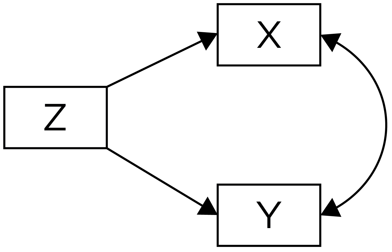
X and Y due to a Common Cause, Z. From Petersen (2024) and Petersen (2025).
Lastly, the association might be spurious (pure coincidence). It might just reflect random variation (i.e., chance), and that when tested on an independent sample, what appeared as an association in the original dataset may not hold when testing the association in a new dataset. Vigen (2024) provides a collection of spurious correlations: https://www.tylervigen.com/spurious-correlations (archived at https://perma.cc/L443-JPRN). As Vigen (2024) notes, spurious correlations may be particularly common in the context of outliers (extreme values), a small sample size, and when performing data dredging (or p-hacking)—i.e., examining the associations among many, many variables.
8.5.3 Case Study
In a case study, we assess a small sample of individuals (commonly only one person or a few people), often with rich qualitative information. Themes may be coded from the qualitative information, which may help inform inferences about whether some process may have played a role in influencing the outcome of interest. The inferences are then drawn in a subjective, qualitative way. Testimonials and anecdotes are examples are case studies.
For instance, to use a case study to evalute the possibilty that players who drink sports drinks perform better than players who drink only water, we could conduct an in-depth interview with a player. In the interview, we might ask the player how they performed in games with versus without a sports drink and have them discuss whether they believe the sports drink improved their performance (and if so, how). Then, based on the player’s responses, we might code the responses to extract themes and to make a qualitative judgement of whether or not the player likely performed better during games in which they had a sports drink.
8.5.4 Other Features of the Research Design
8.5.4.1 Number of Timepoints
In addition to whether the research design is an experiment, correlational/observational study, or a case study, a research design can also have one or multiple timepoints. The differing number of timepoints allow studies to be characterized as one of the following:
- cross-sectional
- longitudinal
8.5.4.1.1 Cross-Sectional
A cross-sectional study is a study with one timepoint.
For instance, in a cross-sectional study evaluating whether having a sports drink improves player performance, we might assess players’ drinking behavior and performance during only game 1.
Cross-sectional studies are more common than longitudinal studies because cross-sectional studies are less costly and time-consuming. They can provide a helpful starting point to test findings more rigorously in subsequent longitudinal studies.
8.5.4.1.2 Longitudinal Design
A longitudinal study is a study with more than one timepoint. When the same measures are assessed at each of multiple timepoints, we refer to this as a “repeated measures” design.
In a longitudinal study evaluating whether having a sports drink improves player performance, we might assess players’ drinking behavior and performance during each game of the season, and possibly across multiple seasons.
Longitudinal studies are less common than cross-sectional studies because longitudinal studies are more costly and time-consuming. Nevertheless, longitudinal studies can allow us test our hypotheses more rigorously, because they can allow us to test whether changes in the predictor/indepdnent variable leads to changes in the outcome/dependent variable. Thus, compared to cross-sectional studies, longitudinal studies can provide greater confidence in causal inferences.
8.5.4.2 Within- or Between-Subject
A research design can also be within-subject, between-subject, or both. A study can involve both within-subject and between-subject comparisons if one predictor/independent variable is within-subject and another predictor/independent variable is between-subject.
8.5.4.2.1 Within-Subject Design
A within-subject design is one in which each participant (i.e., person or player) receives multiple levels of the independent variable (or predictor).
For instance, in an experiment evaluating whether having a sports drink improves player performance, we might assign players to drink the sports drink in the first half of the game and to drink only water in the second half of the game. Or we could assign some of the players to drink sports drink in the first half and water in the second half, and assign the other players to drink water in the first half and sports drink in the second half.
In a correlational study evaluating whether having a sports drink improves player performance, we might evaluate how within-person changes in sports drink consumption are associated with within-person changes in performance. That is, we could evaluate, when a given player has a sports drink (or more sports drinks), do they perform better than when the same individual has only water (or fewer sports drinks)?
Within-subject designs tend to have greater statistical power than between-subject designs. However, within-subject designs often have carryover effects. For instance, consider the study in which we assign players to drink only water in the first and third quarters and to drink sports drink in the second and fourth quarters (an A-B-A-B design). Drinking sports drink in the second quarter could increase how much hydration a player has throughout the rest of the game, which could lead to altered performance in the third and fourth quarters that is not due to what they drink in third and fourth quarters.
8.5.4.2.2 Between-Subject Design
A between-subject design is one in which each participant (i.e., person or player) receives only one level of the independent variable.
For instance, in an experiment evaluating whether having a sports drink improves player performance, we might assign some players to drink the sports drink but the other players to drink only water.
In a correlational study evaluating whether having a sports drink improves player performance, we might evaluate whether people who drink sports drinks tend to perform better than players who drink only water. Or, we could evaluate whether players who drink more sports drinks perform better than players who drink fewer sports drinks (i.e., whether the number of sports drinks consumed during a game is correlated with player performance).
8.6 Research Design Validity
Research design validity involves the accuracy of inferences from a study. There are three types of research design validity:
- internal validity
- external validity
- conclusion validity
8.6.1 Internal Validity
Internal validity is the extent to which we can be confident that the associations identified in the study are causal.
8.6.2 External Validity
External validity is the extent to which we can be confident that findings from the study play out similarly in the real world—that is, the findings generalize to the target population.
8.6.3 Tradeoffs Between Internal and External Validity
There is a tradeoff between internal and external validity—a single research design cannot have both high internal and high external validity. Each study and design has weaknesses. Some research designs are better suited for making causal inferences, whereas other designs tend to be better suited for making inferences that generalize to the real world. The research design that is best suited to making causal inferences is an experiment because it is the design in which the researcher has the greatest control over the variables. Thus, experiments tend to have higher internal validity than other research designs. However, by manipulating one variable and holding everything else constant, the research takes place in a very standardized fashion that can become like studying a process in a vacuum. So, even if a process is theoretically causal in a vacuum, it may act differently in the real world when it interacts with other processes.
Correlational designs have greater capacity for external validity than experimental designs because the participants can be observed in their natural environments to evaluate how variables are related in the real world. However, the greater external validity comes at a cost of lower internal validity. Correlational designs are not well-positioned to make causal inferences. Correlational studies can account for potential confounds using covariates or for the reverse direction of effect using longitudinal designs, but the researcher has less control over the variables than in an experiment.
As the internal validity of a study’s design increases, its external validity tends to decrease. The greater control we have over variables (and, therefore, have greater confidence about causal inferences), the lower the likelihood that the findings reflect what happens in the real world because it is studying things in a metaphorical vacuum. Because no single research design can have both high internal and external validity, scientific inquiry needs a combination of many different research designs so we can be more confident in our inferences—experimental designs for making causal inferences and correlational designs for making inferences that are more likely to reflect the real world.
Case studies, because they have smaller sample sizes and inferences drawn in a subjective, qualitative way, tend to have lower external validity than both experimental and correlational studies. Case studies also tend to have lower internal validity because they have less control over variables, and thus fail to remove the possibility of illusory correlations, potential confounds, or the reverse direction of effect. Thus, case studies are among the weakest forms of evidence. Nevertheless, case studies can still be useful for generating hypotheses that can then be tested empirically with a larger sample in experimental or correlational studies.
8.6.4 Conclusion Validity
Conclusion validity is the extent to which a study’s conclusions are reasonable about the association among variables based on the data. That is, were the correct statistical analyses performed, and are the interpretations of the findings from those analyses correct?
8.7 Mediation vs Moderation
Both types of effects involve (at least) three variables:
- An independent/predictor variable, which will be labeled as
X. - A dependent/outcome variable, which will be labeled as
Y. - The mediator or moderator variable, which will be labeled as
M.
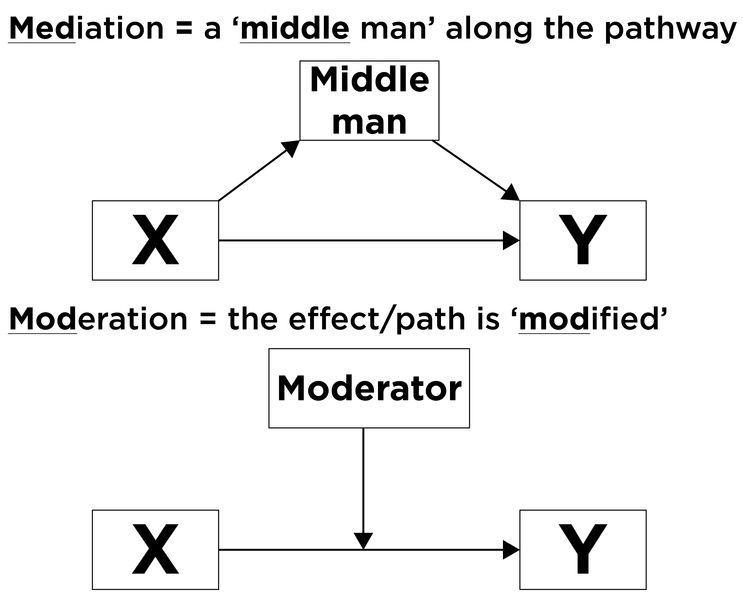
A mnemonic to help remember the difference between mediation and moderation is in Figure 8.5.
8.7.1 Mediation
8.7.1.1 Overview
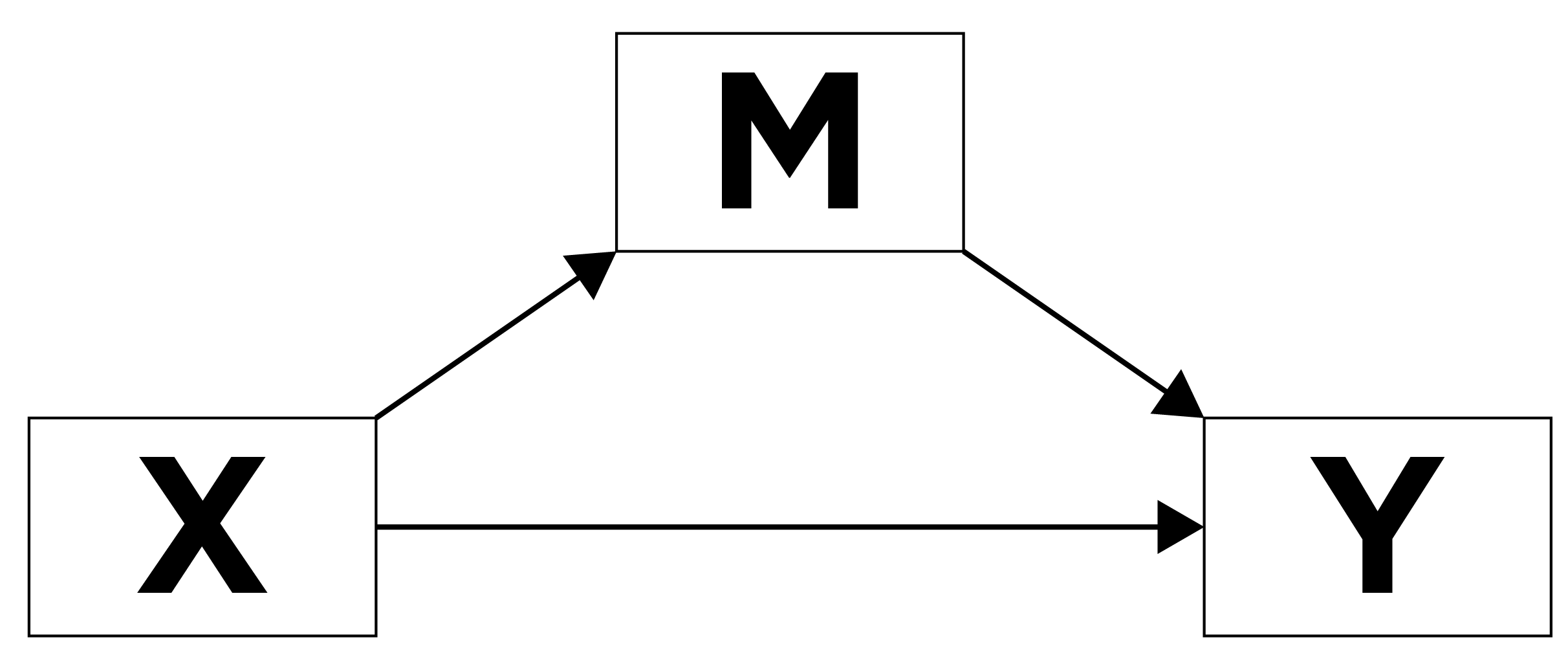
Mediation is a causal chain of events, where one variable (a mediator variable) at least partially explains (or accounts for) the association between two other variables (the predictor variable and the outcome variable). In mediation, a predictor (X) leads to a mediator (M), which leads to an outcome (Y). Mediation answers the question of, “Why (or how) does X influence Y?” A mediator (M) is a variable that helps explain the association between two other variables, and it answers the question of why/how X influences Y. That is, the mediator is the variable that helps explain how/why X is related to Y. In other words, you can think of the mediator as the mechanism that helps explain why X has an impact on Y. The association between X and Y gets smaller when accounting for M. Visually this can be written as in Figure 8.6:

where X is causing M, which in turn is causing Y. In other words, X leads to M, and M leads to Y.
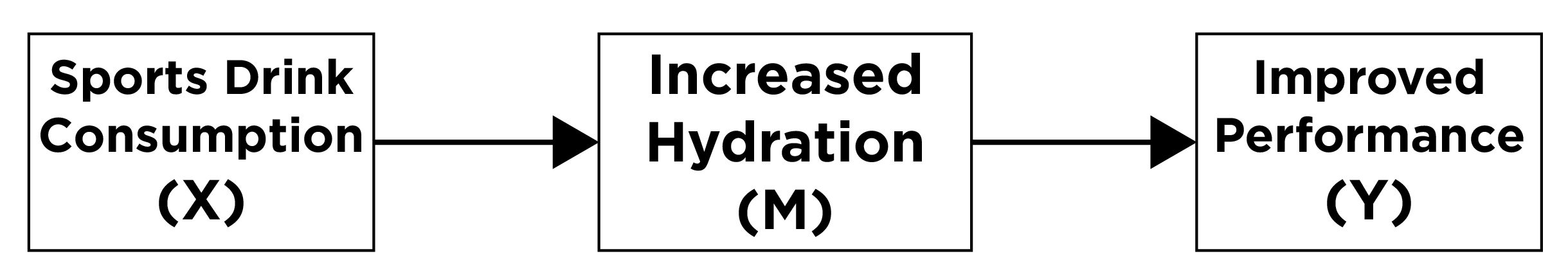
For instance, if we determine that consuming sports drinks improves player performance, we may want to know how/why. That is, what is the mechanism that leads consumption of sports drinks to improve player performance? We might hypothesize that consumption of sports drink helps increase a player’s hydration, which in turn will improve the player’s performance. In this case, increased hydration mediates (i.e., helps explain or account for) the effect of the sports drink consumption on improved player performance.
Question: Why/how does sports drink consumpion lead players to perform better?
Answer: increased hydration
As a picture, we can draw this assocation as in Figure 8.7:
8.7.1.2 Types of Mediation
8.7.1.2.1 Full Mediation
When one mechanism fully accounts for the effect of the predictor variable on the outcome variable, this is known as full mediation, as depicted in Figure 13.15:
8.7.1.2.2 Partial Mediation
When a single process partially—but does not fully—accounts for the effect of the predictor variable on the outcome variable; this is known as partial mediation and is depicted in Figure 13.16:
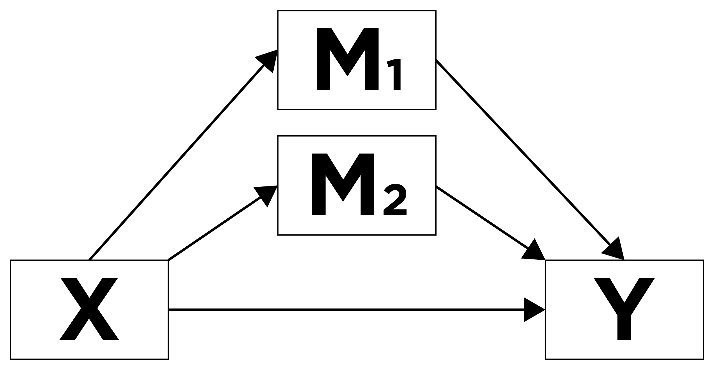
8.7.1.2.3 Multiple Mediators
In addition, there can be multiple mediators/mechanisms that account for the effect of a predictor variable on an outcome variable, as depicted in Figure 8.10:
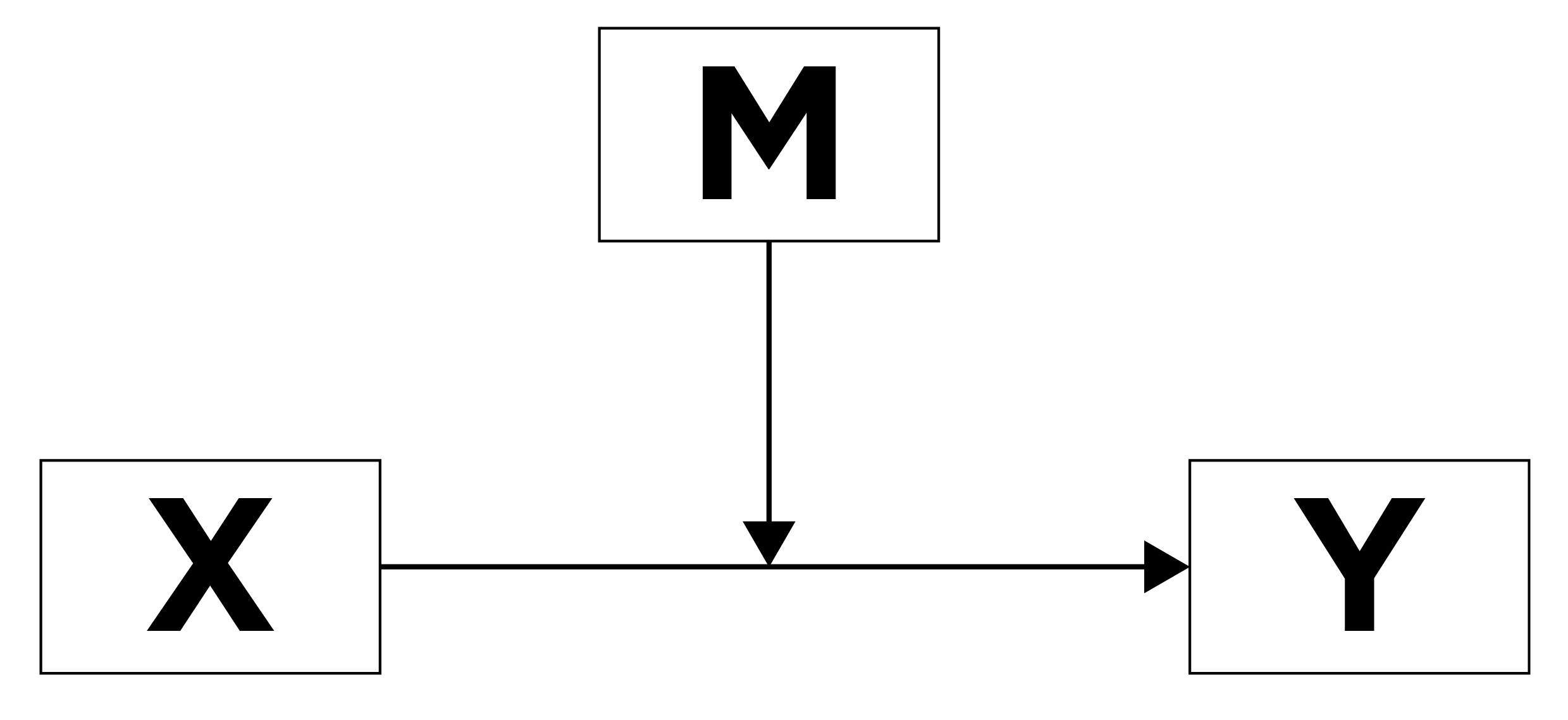
8.7.2 Moderation (i.e., Interaction)
8.7.2.1 Overview
Moderation (sometimes called an “interaction”), on the other hand, occurs when there is a variable or condition (M; called a “moderator”) that changes the association between X and Y. That is, the effect of the predictor variable on the outcome variable differs at different levels of the moderator variable. In these cases, X and M work together to have an effect on Y; here X does not have a direct effect on M. Moderation answers the question of, “For whom does X influence Y?” If X influences Y more strongly for some people or in some circumstances, we would say that there is an interaction such that the effect of X on Y depends on M, as depicted in Figure 8.11:
For example, if the effect of consuming sports drinks on player performance differs for Quarterbacks and Wide Receivers, the interaction could be depicted in Figures 8.12 and 8.13:
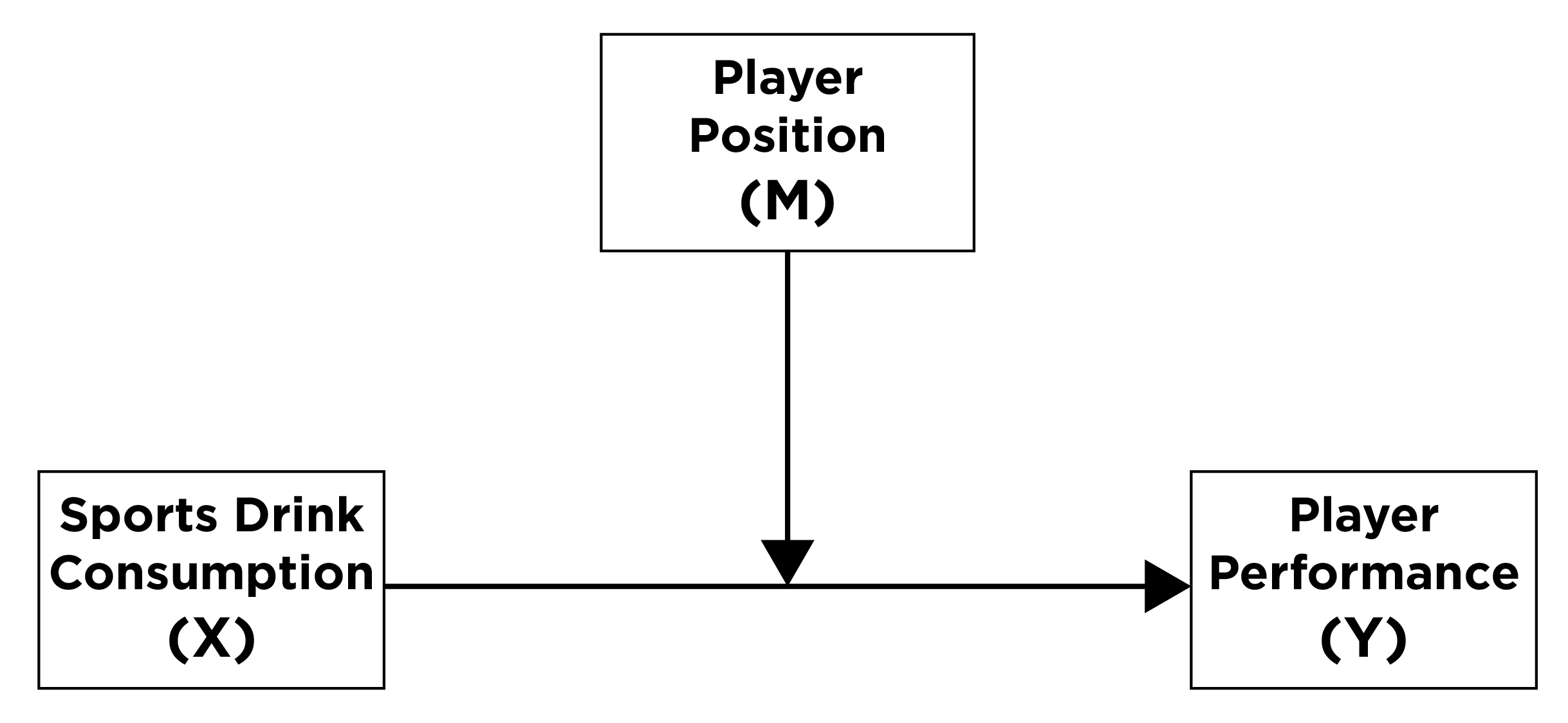
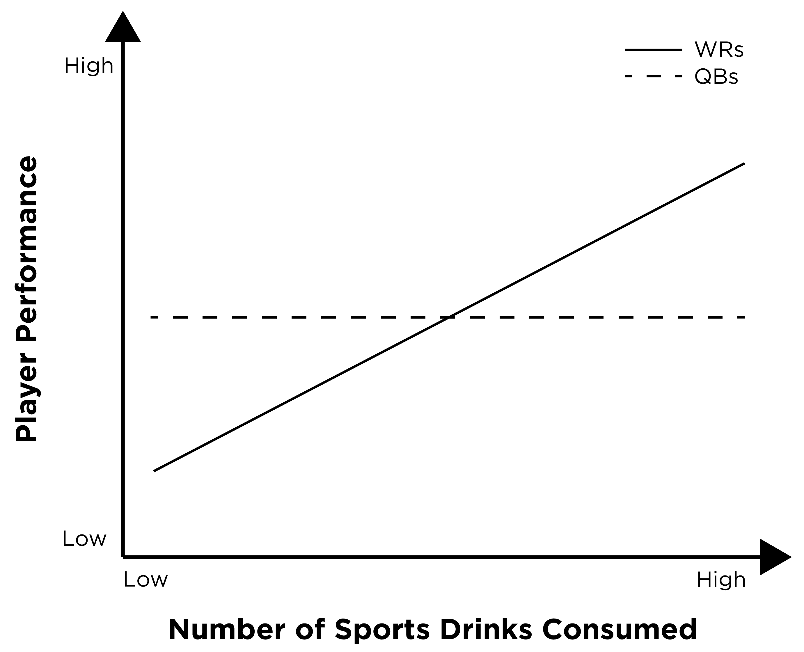
An interaction can be identified visually by non-parallel lines at different levels of the moderator. In this example, the player’s position moderates the effect consuming sports drinks on player performance. In particular, there is a strong positive association between consuming sports drinks and player performance for Wide Receivers (as evidenced by the upward slope of the best-fit regression line), whereas there is no association between consuming sports drinks and player performance for Quarterbacks (as evidenced by the flat line).
8.8 Levels of Measurement
It is important to know the levels of measurement of your data, because the level(s) of measurement of your data constrain the types of comparisons and analyses that you can meaningfully perform. There are four levels of measurement that any variable can have:
- nominal
- ordinal
- interval
- ratio
Each is described below:
8.8.1 Nominal
A variable is considered nominal if it is composed of qualitative classifications. You cannot meaningfully evaluate whether one number in the variable is larger than another number in the variable because higher numbers do not reflect higher levels of the concept. Examples of nominal variables include:
- sex (e.g., 1 = male; 2 = female)
- race (e.g., 1 = American Indian; 2 = Asian; 3 = Black; 4 = Pacific Islander; 5 = White)
- ethnicity (e.g., 0 = Non-Hispanic/Latino; 1 = Hispanic/Latino)
- zip code
- jersey number
A football player’s jersey number is an example of a nominal variable. A jersey number of 7 is not higher on whatever concept of interest compared to a jersey number of 6.
To examine the central tendency of a nominal variable, you can determine the mode, but you cannot calculate a mean or median.
8.8.2 Ordinal
A variable is considered ordinal if the classifications are ordered. However, ordinal variables do not have equally spaced intervals. Examples of ordinal intervals include:
- likert response scales (e.g., 1 = strongly disagree; 2 = disagree; 3 = neutral; 4 = agree; 5 = strongly agree)
- educational attainment (e.g., 1 = no formal education; 2 = elementary school; 3 = middle school; 4 = high school; 5 = college; 6 = graduate degree)
- academic grades on A–F scale (e.g., 1 = A; 2 = B; 3 = C; 4 = D; 5 = F)
- player rank (1 = 1st; 2 = 2nd; 3 = 3rd, etc.)
A football player’s fantasy rank is an example of an ordinal variable. A player with a fantasy rank of 1 has a higher rank than a player with a rank of 2, but it is not known how far apart each player is—i.e., the intervals do not all reflect the same distance. For instance, the distance between the top-ranked player and the 2nd-best player might be 30 points, whereas the distance between the 2nd-best player and the 3rd-best player might be 2 points.
To examine the central tendency of ordinal data, the median and mode are most appropriate; however, the mean may be used (unlike for nominal data).
8.8.3 Interval
A variable is considered interval if the classifications are ordered (similar to ordinal data) and have equally spaced intervals (unlike ordinal data). However, interval variables do not have a meaningful zero that reflects absence. Examples of interval data include:
- temperature on the Fahrenheit or Celsius scale
- time of day
For instance, the temperature difference between 80 and 90 degrees Fahrenheit is the same as the temperature difference between 90 and 100 degrees Fahrenheit. However, 0 degrees Fahrenheit does not reflect absence of temperature/heat.
Interval data can be meaningfully added or subtracted. For instance, if a game starts at 4 pm and ends at 7 pm, you know the game lasted 3 hours (\(7 - 4 = 3\)). However, interval data cannot be meaningfully multiplied or divided. For instance, 100 degrees Fahrenheit is not twice as hot as 50 degrees Fahrenheit.
To examine the central tendency of interval data, you can compute the mean, median, or mode.
8.8.4 Ratio
A variable is considered ratio if the classifications are ordered (similar to ordinal data), have equally spaced intervals (like interval data), and have an absolute zero point that reflects absence of the concept. Examples of ratio data include:
- temperature on the Kelvin scale
- height
- weight
- age
- distance
- speed
- volume
- time elapsed
- income
- stock price
- years of formal education
- points in football
For instance, points in football has order, equally spaced intervals, and an absolute zero—a team cannot score less than zero points, and zero points reflects absence of points (though it could be argued to be interval data because zero points does not reflect absence of skill.)
Ratio data can be meaningfully added, subtracted, multiplied, or divided. A player who weighs 350 pounds weighs twice as much as someone who weighs 175 pounds.
To examine the central tendency of ratio data, you can compute the mean, median, or mode.
8.9 Psychometrics
Below, I provide brief discussions of various aspects of measurement reliability and validity. For more information on these and other aspects of psychometrics, see Petersen (2024) and Petersen (2025).
8.9.1 Measurement Reliability
The reliability of a measure’s scores deals with the consistency of measurement. This book focuses on the following types of reliability:
- test–retest reliability
- inter-rater reliability
- intra-rater reliability
- internal consistency
- parallel-forms reliability
For more information on these and other aspects of reliability, see https://isaactpetersen.github.io/Principles-Psychological-Assessment/reliability.html (Petersen, 2024, 2025). Reliability is important to consider because random measurement error (i.e., unreliability) weakens the associations between variables (Goodwin & Leech, 2006; Schmidt & Hunter, 1996).
8.9.1.1 Test–Retest Reliability
Test–retest reliability evaluates the consistency of scores across time. For a construct that is expected to be stable across time (e.g., hand size in adults), we would expect our measurements to be consistent across time. The consistency of scores across time can be examined in terms of relative or absolute test–retest reliability. Relative test–retest reliability—i.e., the consistency of individual differences across time—is commonly evaluated using the coefficient of stability (i.e., the Pearson correlation coefficient). Absolute test–retest reliability—i.e., the absolute consistency of people’s scores across time—is commonly evaluated using the coefficient of repeatability and the coefficient of agreement (i.e., intraclass correlation coefficient).
8.9.1.2 Inter-Rater Reliability
Inter-rater reliability evaluates the consistency of scores across raters. For instance, if we have a strong measure for assessing college players’ aptitude to succeed in the NFL, the measure should yield a similar score for a given player regardless of which (trained) rater (e.g., coach or talent scout) uses it to rate the player. The consistency of scores across raters is commonly evaluated using the intraclass correlation coefficient (for continuous variables) and Cohen’s kappa (\(\kappa\); for categorical variables).
8.9.1.3 Intra-Rater Reliability
Intra-rater reliability evaluates the consistency of scores within a given rater. If we have a strong measure for assessing college players’ aptitude to succeed in the NFL, the measure should yield a similar score for a given player from the same (trained) rater (e.g., coach or talent scout) each time they rate the same player (assuming the player’s aptitude has not changed). The consistency of scores within raters can be evaluated using similar approaches as those evaluating inter-rater reliability.
8.9.1.4 Internal Consistency
Internal consistency evaluates the consistency of scores across items within a measure. If we develop a strong questionnaire measure to assess a college players’ aptitude to succeed in the NFL, the scores should be relatively consistent across items. The consistency of scores across items within a measure is commonly evaluated using Cronbach’s alpha (\(\alpha\)) or McDonald’s omega (\(\omega\)).
8.9.1.5 Parallel-Forms Reliability
Parallel-forms reliability evaluates the consistency of scores across different but equivalent forms of a measure. If we develop two equivalent versions of the Wonderlic Contemporary Cognitive Ability Test (Form A and Form B) so that players sitting next to each other do not receive the same items, we would expect a player’s score on Form A would be similar to their score on Form B. Parallel-forms reliability is is commonly evaluated using the coefficient of equivalence (i.e., the Pearson correlation coefficient).
8.9.2 Measurement Validity
The validity of a measure’s scores deals with the accuracy of measurement. This book focuses on the following types of validity:
- face validity
- content validity
- criterion-related validity
- construct validity
- convergent validity
- discriminant validity
- incremental validity
- ecological validity
For more information on these and other aspects of validity, see https://isaactpetersen.github.io/Principles-Psychological-Assessment/validity.html (Petersen, 2024, 2025).
8.9.2.1 Face Validity
Face validity evaluates the extent to which a measure “looks like” (on its face) it assesses the construct of interest. For instance, if a measure is developed to assess aptitude of Wide Receivers for the position, it would be considered to have face validity if everyday (lay) people believe that it assesses aptitude for being a successful Wide Receiver.
8.9.2.2 Content Validity
Content validity evaluates the extent to which the measure assesses the full breadth of the content, as determined by context experts. For the measure to have content validity, it should not have gaps (missing content facets) or intrusions (facets of other constructs). For instance, a strong measure for assessing a player’s aptitude to succeed in the NFL might need to include a player’s speed, strength, size, lateral quickness, etc. If the measure is missing their speed, this would be a content gap. If the measure assesses a construct-irrelevant facet (e.g., their attractiveness), this would be a content intrusion.
8.9.2.3 Criterion-Related Validity
Criterion-related validity evaluates the extent to which the measure’s scores are related to meaningful variables of interest. Criterion-related validity is commonly evaluated using a Pearson correlation or some form of regression.
There are two types of criterion-related validity:
- concurrent (criterion-related) validity
- predictive (criterion-related) validity
8.9.2.3.1 Concurrent (Criterion-Related) Validity
Concurrent criterion-related validity (aka concurrent validity) evaluates the extent to which the measure’s scores are related to meaningful variables of interest assessed at the same point in time. That is, concurrent validity could evaluate whether current player statistics (e.g., passing yards) are associated with their fantasy points.
8.9.2.3.2 Predictive (Criterion-Related) Validity
Predictive criterion-related validity (aks predictive validity) evaluates the extent to which the measure’s scores are related to meaningful variables of interest that are assessed at a later point in time. For example, predictive validity could evaluate whether scores on the measure we developed to assess a player’s aptitude to succeed in the NFL predicts later performance in the NFL.
8.9.2.4 Construct Validity
Construct validity evaluates the extent to which the measure’s scores accurately assess the construct of interest. If we develop a measure with intent to assess aptitude for being a successful Running Back, and it appears to more accurately assess aptitude for being a successful Wide Receiver, then our measure has poor construct validity for assessing aptitude for being a successful Running Back. Construct validity subsumes convergent and discriminant validity, in addition to all of the other forms of measurement validity.
8.9.2.5 Convergent Validity
Convergent validity evaluates the extent to which the measure’s scores are related to other measures of the same construct. For instance, if we develop a new measure to assess intelligence, its scores should be related to scores from other measures designed to assess intelligence (e.g., Wonderlic Contemporary Cognitive Ability Test).
8.9.2.6 Discriminant Validity
Discriminant validity evaluates the extent to which the measure’s scores are unrelated to measures of the different constructs. For instance, if we develop a new measure to assess intelligence, its scores should be less strongly associated with measures of other constructs (e.g., measures of happiness).
8.9.2.7 Incremental Validity
Incremental validity evaluates the extent to which the measure’s scores provide an increase in predictive accuracy compared to other information that is easily and cheaply available. That is, in order to be useful, a strong measure should tell us something that we did not already know. For instance, if we develop a strong measure of intelligence, it should result in increased predictive accuracy (for success in the NFL) compared to when just relying on the Wonderlic Contemporary Cognitive Ability Test.
8.9.2.8 Ecological Validity
Ecological validity evaluates the extent to which the measures’ scores are indicative of the behavior of a person in the natural environment. For instance, measures of a players’ speed during a game has higher ecological validity (and is more predictive of their performance) than their speed during the NFL Combine (Lyons et al., 2011). For instance, compared to tests of speed, power, and agility at the NFL Combine, collegiate performance is a stronger predictor of performance in the NFL (Lyons et al., 2011). That is, previous sports performance is the best predictor of future performance (for a review, see Den Hartigh et al., 2018).
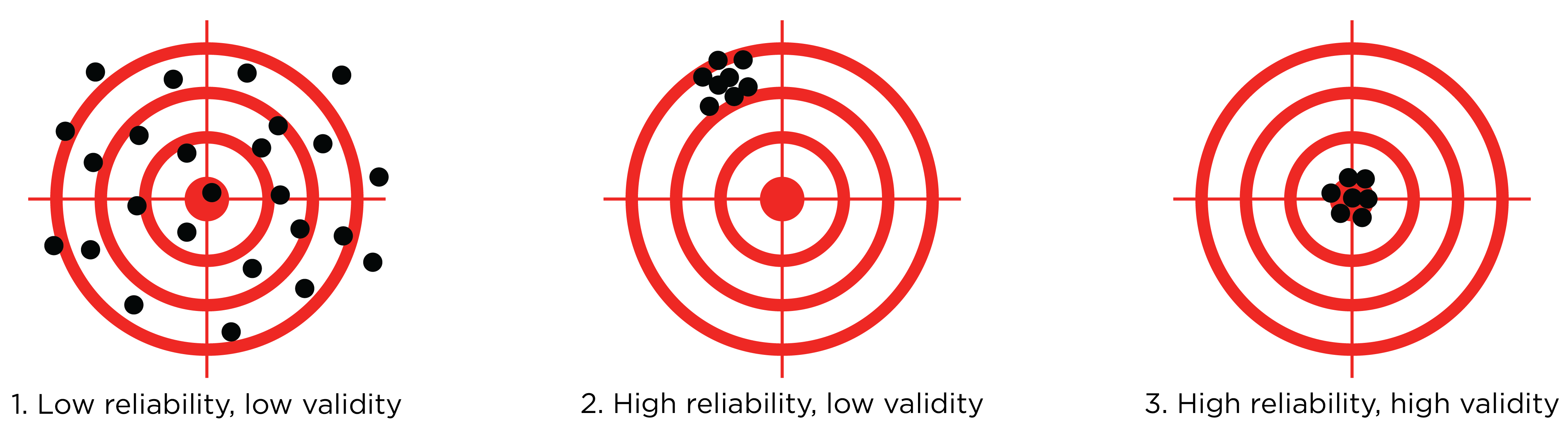
8.9.3 Reliability vs Validity
Reliability and validity are different but related. Reliability refers to the consistency of scores, whereas accuracy refers to the accuracy of scores. Validity depends on reliability. Reliability is necessary—but insufficient for—validity. That is, consistency is necessary—but insufficient for—accuracy. As depicted in Figure 8.14, a measure can be no more valid than it is reliable. A measure can be consistent but inaccurate; however, a measure cannot be accurate but inconsistent.
8.10 Conclusion
There are various types of research designs. Each type of research design differs in the extent to which it supports the ability to draw causal inferences (internal validity) versus the extent to which it supports the ability to identify processes that generalize to the real-world (external validity). In addition, it is important to understand the distinction between sample and population, and the distinction between mediation and moderation. It is also important to consider the levels of measurement used because they constrain the types of analyses that may be performed. In addition, it is important to consider the psychometrics of measurements, including multiple aspects of reliability (consistency) and validity (accuracy).