I want your feedback to make the book better for you and other readers. If you find typos, errors, or places where the text may be improved, please let me know. The best ways to provide feedback are by GitHub or hypothes.is annotations.
You can leave a comment at the bottom of the page/chapter, or open an issue or submit a pull request on GitHub: https://github.com/isaactpetersen/Fantasy-Football-Analytics-Textbook
Alternatively, you can leave an annotation using hypothes.is.
To add an annotation, select some text and then click the
symbol on the pop-up menu.
To see the annotations of others, click the
symbol in the upper right-hand corner of the page.
22 Factor Analysis
“All models are wrong, but some are useful.”
— George Box (1979, p. 202)
This chapter provides an overview of factor analysis, which encompasses a range of latent variable modeling approaches, including exploratory and confirmatory factor analysis.
22.1 Getting Started
22.1.1 Load Packages
22.1.2 Load Data
We created the player_stats_weekly.RData and player_stats_seasonal.RData objects in Section 4.4.3.
22.1.3 Prepare Data
22.1.3.1 Season-Averages
Code
player_stats_seasonal_avgPerGame <- player_stats_seasonal %>%
  mutate(
    completionsPerGame = completions / games,
    attemptsPerGame = attempts / games,
    passing_yardsPerGame = passing_yards / games,
    passing_tdsPerGame = passing_tds / games,
    passing_interceptionsPerGame = passing_interceptions / games,
    sacks_sufferedPerGame = sacks_suffered / games,
    sack_yards_lostPerGame = sack_yards_lost / games,
    sack_fumblesPerGame = sack_fumbles / games,
    sack_fumbles_lostPerGame = sack_fumbles_lost / games,
    passing_air_yardsPerGame = passing_air_yards / games,
    passing_yards_after_catchPerGame = passing_yards_after_catch / games,
    passing_first_downsPerGame = passing_first_downs / games,
    #passing_epaPerGame = passing_epa / games,
    #passing_cpoePerGame = passing_cpoe / games,
    passing_2pt_conversionsPerGame = passing_2pt_conversions / games,
    #pacrPerGame = pacr / games
    pass_40_ydsPerGame = pass_40_yds / games,
    pass_incPerGame = pass_inc / games,
    #pass_comp_pctPerGame = pass_comp_pct / games,
    fumblesPerGame = fumbles / games
  )

nfl_nextGenStats_seasonal <- nfl_nextGenStats_weekly %>%
  filter(season_type == "REG") %>%
  select(-any_of(c("week","season_type","player_display_name","player_position","team_abbr","player_first_name","player_last_name","player_jersey_number","player_short_name"))) %>%
  group_by(player_gsis_id, season) %>%
  summarise(
    across(everything(),
      ~ mean(.x, na.rm = TRUE)),
    .groups = "drop")
22.1.3.2 Merge Data
22.1.3.3 Specify Variables
Code
faVars <- c(
 "completionsPerGame","attemptsPerGame","passing_yardsPerGame","passing_tdsPerGame",
 "passing_air_yardsPerGame","passing_yards_after_catchPerGame","passing_first_downsPerGame",
 "avg_completed_air_yards","avg_intended_air_yards","aggressiveness","max_completed_air_distance",
 "avg_air_distance","max_air_distance","avg_air_yards_to_sticks","passing_cpoe","pass_comp_pct",
 "passer_rating","completion_percentage_above_expectation"
)
22.1.3.4 Subset Data
22.1.3.5 Standardize Variables
Standardizing variables is not strictly necessary in factor analysis; however, standardization can be helpful to prevent some variables from having considerably larger variances than others.
22.2 Overview of Factor Analysis
Factor analysis involves the estimation of latent variables. Latent variables are ways of studying and operationalizing theoretical constructs that cannot be directly observed or quantified. Factor analysis is a class of latent variable models that is designated to identify the structure of a measure or set of measures, and ideally, a construct or set of constructs. It aims to identify the optimal latent structure for a group of variables. The goal of factor analysis is to identify simple, parsimonious factors that underlie the “junk” (i.e., scores filled with measurement error) that we observe. That is, similar to principal component analysis, factor analysis can help us perform data reduction—i.e., it can help us reduce down a larger set of variables into a smaller set of factors.
Factor analysis encompasses two general types: confirmatory factor analysis and exploratory factor analysis. Exploratory factor analysis (EFA) is a latent variable modeling approach that is used when the researcher has no a priori hypotheses about how a set of variables is structured. EFA seeks to identify the empirically optimal-fitting model in ways that balance accuracy (i.e., variance accounted for) and parsimony (i.e., simplicity). Confirmatory factor analysis (CFA) is a latent variable modeling approach that is used when a researcher wants to evaluate how well a hypothesized model fits, and the model can be examined in comparison to alternative models. Using a CFA approach, the researcher can pit models representing two theoretical frameworks against each other to see which better accounts for the observed data.
Factor analysis involves observed (manifest) variables and unobserved (latent) factors. Factor analysis assumes that the latent factor influences the manifest variables, and the latent factor therefore reflects the common variance among the variables. A factor model potentially includes factor loadings, residuals (errors or disturbances), intercepts/means, covariances, and regression paths. When depicting a factor analysis model, rectangles represent variables we observe (i.e., manifest variables), and circles represent latent (i.e., unobserved) variables. A regression path indicates a hypothesis that one variable (or factor) influences another, and it is depicted using a single-headed arrow. The standardized regression coefficient (i.e., beta or \(\beta\)) represents the strength of association between the variables or factors. A factor loading is a regression path from a latent factor to an observed (manifest) variable. The standardized factor loading represents the strength of association between the variable and the latent factor, where conceptually, it is intended to reflect the magnitude that the latent factor influences the observed variable. A residual is variance in a variable (or factor) that is unexplained by other variables or factors. A variable’s intercept is the expected value of the variable when the factor(s) (onto which it loads) is equal to zero. A covariance is the unstandardized index of the strength of association between two variables (or factors), and it is depicted with a double-headed arrow.
Because a covariance is unstandardized, its scale depends on the scale of the variables. The covariance between two variables is the average product of their deviations from their respective means, as in Equation 10.1. The covariance of a variable with itself is equivalent to its variance, as in Equation 10.2. By contrast, a correlation is a standardized index of the strength of association between two variables. Because a correlation is standardized (fixed between [−1,1]), its scale does not depend on the scales of the variables. Because a covariance is unstandardized, its scale depends on the scale of the variables. A covariance path between two variables represents omitted shared cause(s) of the variables. For instance, if you depict a covariance path between two variables, it means that there is a shared cause of the two variables that is omitted from the model (for instance, if the common cause is not known or was not assessed).
In factor analysis, the relation between an indicator (\(\text{X}\)) and its underlying latent factor(s) (\(\text{F}\)) can be represented with a regression formula as in Equation 22.1:
\[ X = \lambda \cdot \text{F} + \text{Item Intercept} + \text{Error Term} \tag{22.1}\]
where:
- \(\text{X}\) is the observed value of the indicator
- \(\lambda\) is the factor loading, indicating the strength of the association between the indicator and the latent factor(s)
- \(\text{F}\) is the person’s value on the latent factor(s)
- \(\text{Item Intercept}\) represents the constant term that accounts for the expected value of the indicator when the latent factor(s) are zero
- \(\text{Error Term}\) is the residual, indicating the extent of variance in the indicator that is not explained by the latent factor(s)
When the latent factors are uncorrelated, the (standardized) error term for an indicator is calculated as 1 minus the sum of squared standardized factor loadings for a given item (including cross-loadings). A cross-loading is when a variable loads onto more than one latent factor.
Factor analysis is a powerful technique to help identify the factor structure that underlies a measure or construct. However, given the extensive method variance that influences scores on measure, factor analysis (and principal component analysis) tends to extract method factors. Method factors are factors that are related to the methods being assessed rather than the construct of interest. To better estimate construct factors, it is sometimes necessary to estimate both construct and method factors.
Before pursuing factor analysis, it is helpful to evaluate the extent to which the variables are intercorrelated. If the variables are not correlated (or are correlated only weakly), there is no reason to believe that a common factor influences them, and thus factor analysis would not be useful. So, before conducting a factor analysis, it is important to examine the correlation matrix of the variables to determine whether the variables intercorrelate strongly enough to justify a factor analysis.
22.3 Factor Analysis and Structural Equation Modeling
Factor analysis forms the measurement model component of a structural equation model (SEM). The measurement model is what we settle on as the estimation of each construct before we add the structural component to estimate the relations among latent variables. Basically, in a structural equation model, we add the structural component onto the measurement model. For instance, our measurement model (i.e., based on factor analyis) might be to estimate, from a set of items, three latent factors: usage, aggressiveness, and performance. Our structural model then may examine what processes (e.g., sport drink consumption or sleep) influence these latent factors, how the latent factors influence each other, and what the latent factors influence (e.g., fantasy points). SEM is confirmatory factor analysis with regression paths that specify hypothesized causal relations between the latent variables (the structural component of the model). Exploratory structural equation modeling (ESEM) is a form of SEM that allows for a combination of exploratory factor analysis and confirmatory factor analysis to estimate latent variables and the relations between them.
22.4 Path Diagrams
A key tool when designing a factor analysis or structural equation model is a conceptual depiction of the hypothesized causal processes. A path diagram depicts the hypothesized causal processes that link two or more variables. Path diagrams are an example of a causal diagram and are similar to directed acyclic graphs discussed in Section 13.6. Karch (2025a) provides a tool to create lavaan R syntax from a path analytic diagram: https://lavaangui.org.
In a path analysis diagram, rectangles represent variables we observe, and circles represent latent (i.e., unobserved) variables. Single-headed arrows indicate regression paths, where conceptually, one variable is thought to influence another variable. Double-headed arrows indicate covariance paths, where conceptually, two variables are associated for some unknown reason (i.e., an omitted shared cause).
22.5 Decisions in Factor Analysis
There are five primary decisions to make in factor analysis:
- what variables to include in the model and how to scale them
- method of factor extraction: whether to use exploratory or confirmatory factor analysis
- if using exploratory factor analysis, whether and how to rotate factors
- how many factors to retain (and what variables load onto which factors)
- how to interpret and use the factors
The answer you get can differ highly depending on the decisions you make. Below, we provide guidance for each of these decisions.
22.5.1 1. Variables to Include and their Scaling
The first decision when conducting a factor analysis is which variables to include and the scaling of those variables. What factors you extract can differ widely depending on what variables you include in the analysis. For example, if you include many variables from the same source (e.g., self-report), it is possible that you will extract a factor that represents the common variance among the variables from that source (i.e., the self-reported variables). This would be considered a method factor, which works against the goal of estimating latent factors that represent the constructs of interest (as opposed to the measurement methods used to estimate those constructs).
An additional consideration is the scaling of the variables: whether to use raw variables, standardized variables, or dividing some variables by a constant to make the variables’ variances more similar. Before performing a principal component analysis (PCA), it is generally important to ensure that the variables included in the PCA are on the same scale. PCA seeks to identify components that explain variance in the data, so if the variables are not on the same scale, some variables may contribute considerably more variance than others. A common way of ensuring that variables are on the same scale is to standardize them using, for example, z scores that have a mean of zero and standard deviation of one. By contrast, factor analysis can better accommodate variables that are on different scales.
22.5.2 2. Method of Factor Extraction
22.5.2.1 Exploratory Factor Analysis
Exploratory factor analysis (EFA) is used if you have no a priori hypotheses about the factor structure of the model, but you would like to understand the latent variables represented by your items.
EFA is partly induced from the data. You feed in the data and let the program build the factor model. You can set some parameters going in, including how to extract or rotate the factors. The factors are extracted from the data without specifying the number and pattern of loadings between the items and the latent factors (Bollen, 2002). All cross-loadings are freely estimated.
22.5.2.2 Confirmatory Factor Analysis
Confirmatory factor analysis (CFA) is used to (dis)confirm a priori hypotheses about the factor structure of the model. CFA is a test of the hypothesis. In CFA, you specify the model and ask how well this model represents the data. The researcher specifies the number, meaning, associations, and pattern of free parameters in the factor loading matrix (Bollen, 2002). A key advantage of CFA is the ability to directly compare alternative models (i.e., factor structures), which is valuable for theory testing (Strauss & Smith, 2009). For instance, you could use CFA to test whether the variance in several measures’ scores is best explained with one factor or two factors. In CFA, cross-loadings are not estimated unless the researcher specifies them.
22.5.3 3. Factor Rotation
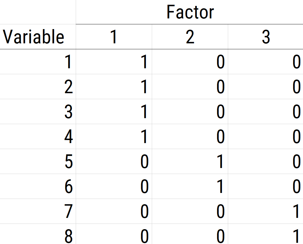
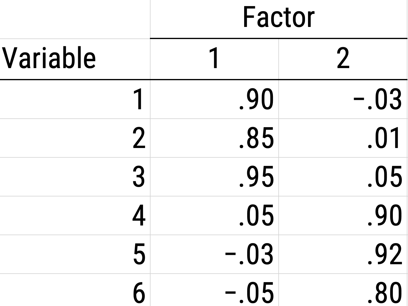
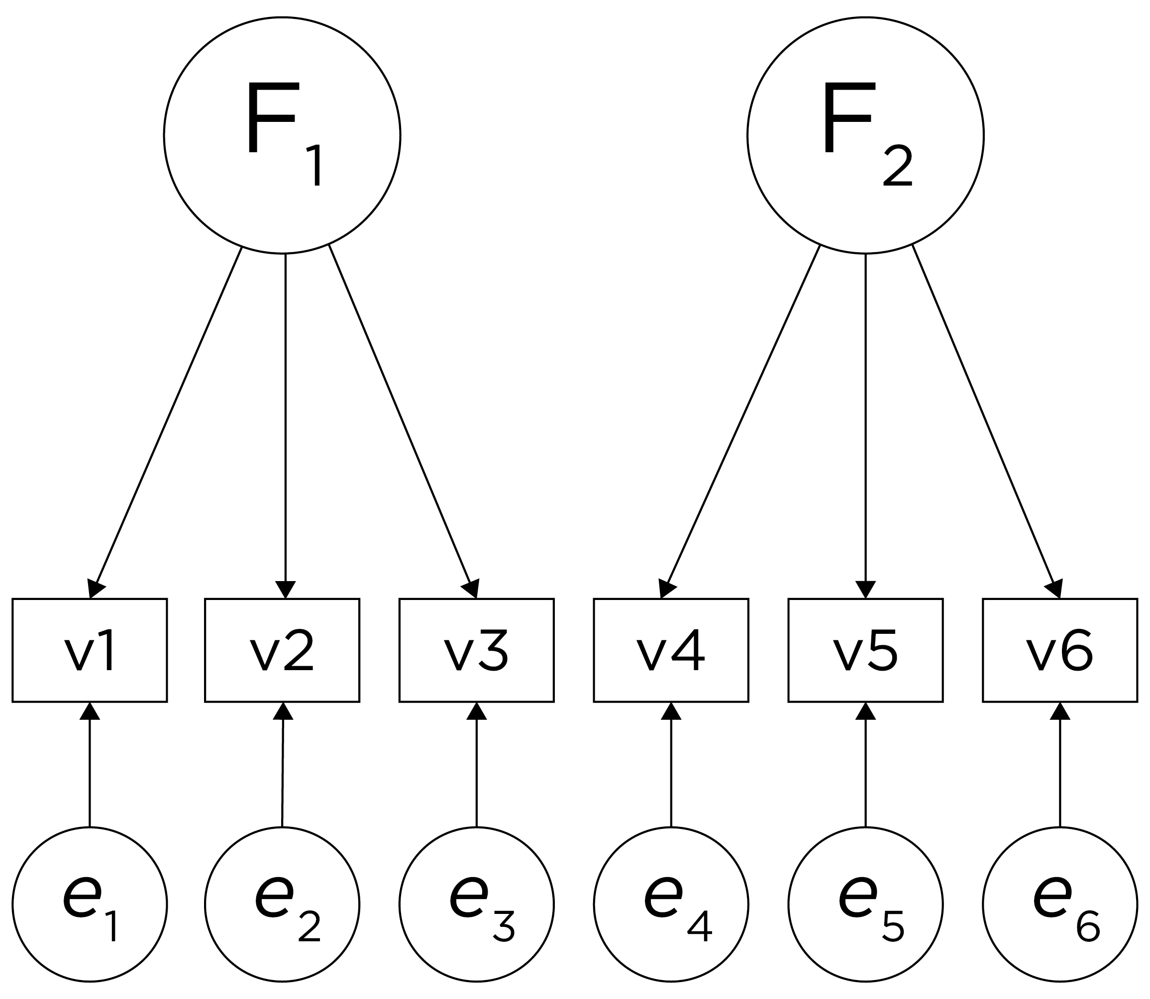
When using EFA or principal component analysis, an important step is, possibly, to rotate the factors to make them more interpretable and simple, which is the whole goal. To interpret the results of a factor analysis, we examine the factor matrix. The columns refer to the different factors; the rows refer to the different observed variables. The cells in the table are the factor loadings—they are basically the correlation between the variable and the factor. Our goal is to achieve a model with simple structure because it is easily interpretable. Simple structure means that every variable loads perfectly on one and only one factor, as operationalized by a matrix of factor loadings with values of one and zero and nothing else. An example of a factor matrix that follows simple structure is depicted in Figure 22.1.
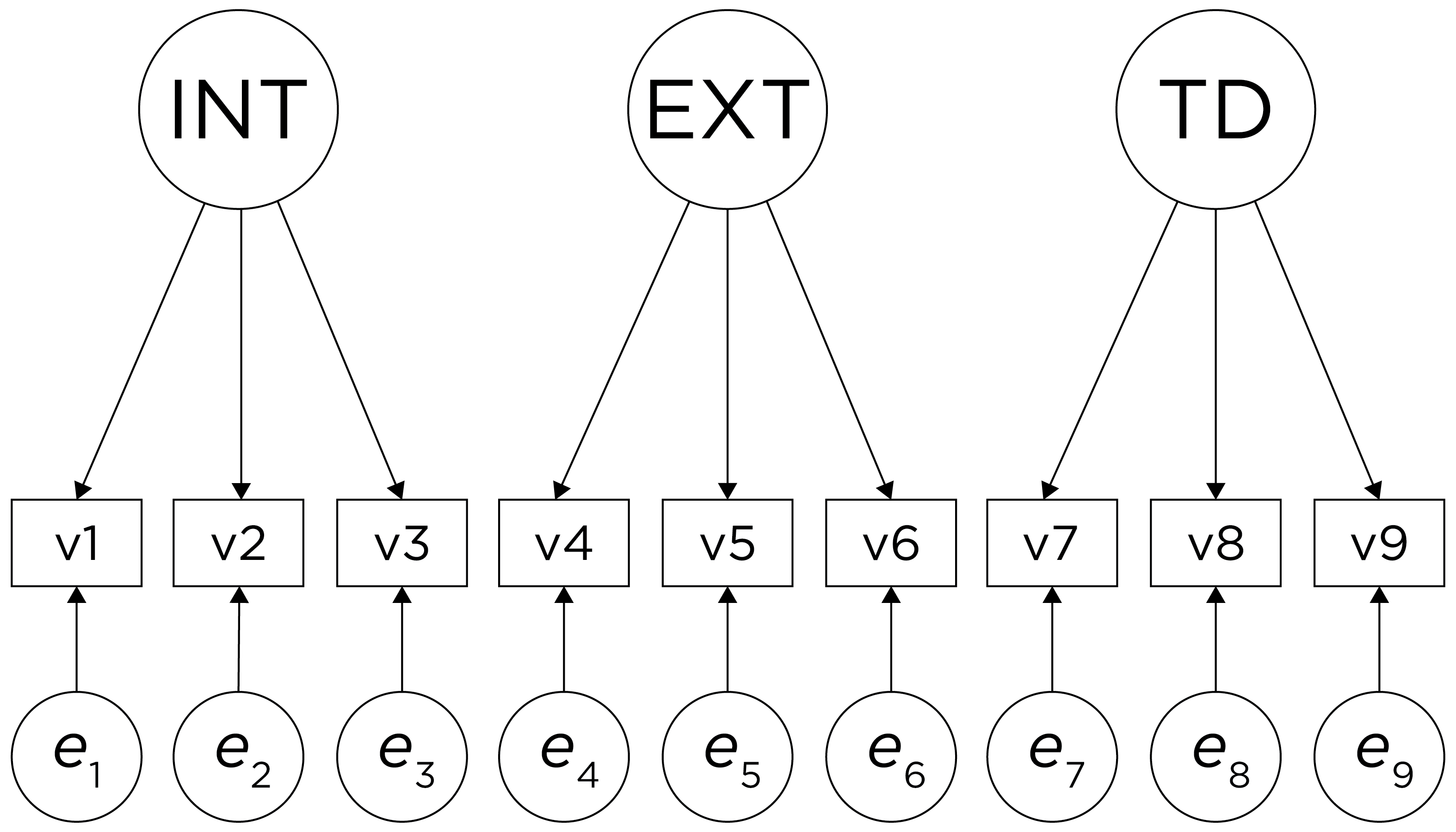
An example of a factor analysis model that follows simple structure is depicted in Figure 22.2. Each variable loads onto one and only one factor, which makes it easy to interpret the meaning of each factor, because a given factor represents the common variance among the items that load onto it.
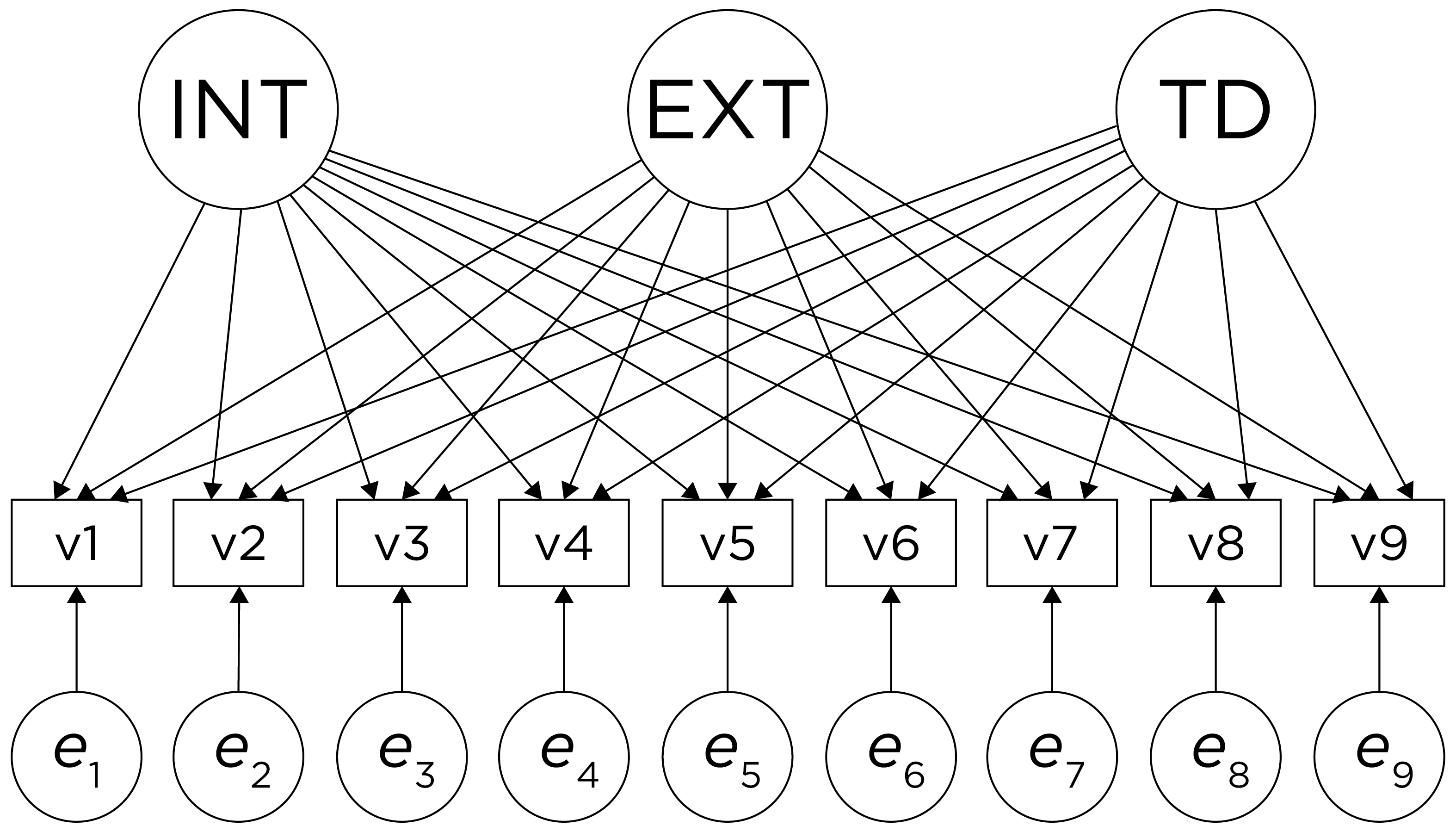
However, pure simple structure only occurs in simulations, not in real-life data. In reality, our unrotated factor analysis model might look like the model in Figure 22.3. In this example, the factor analysis model does not show simple structure because the items have cross-loadings—that is, the items load onto more than one factor. The cross-loadings make it difficult to interpret the factors, because all of the items load onto all of the factors, so the factors are not very distinct from each other, which makes it difficult to interpret what the factors mean.
As a result of the challenges of interpretability caused by cross-loadings, factor rotations are often performed. An example of an unrotated factor matrix is in Figure 22.4.
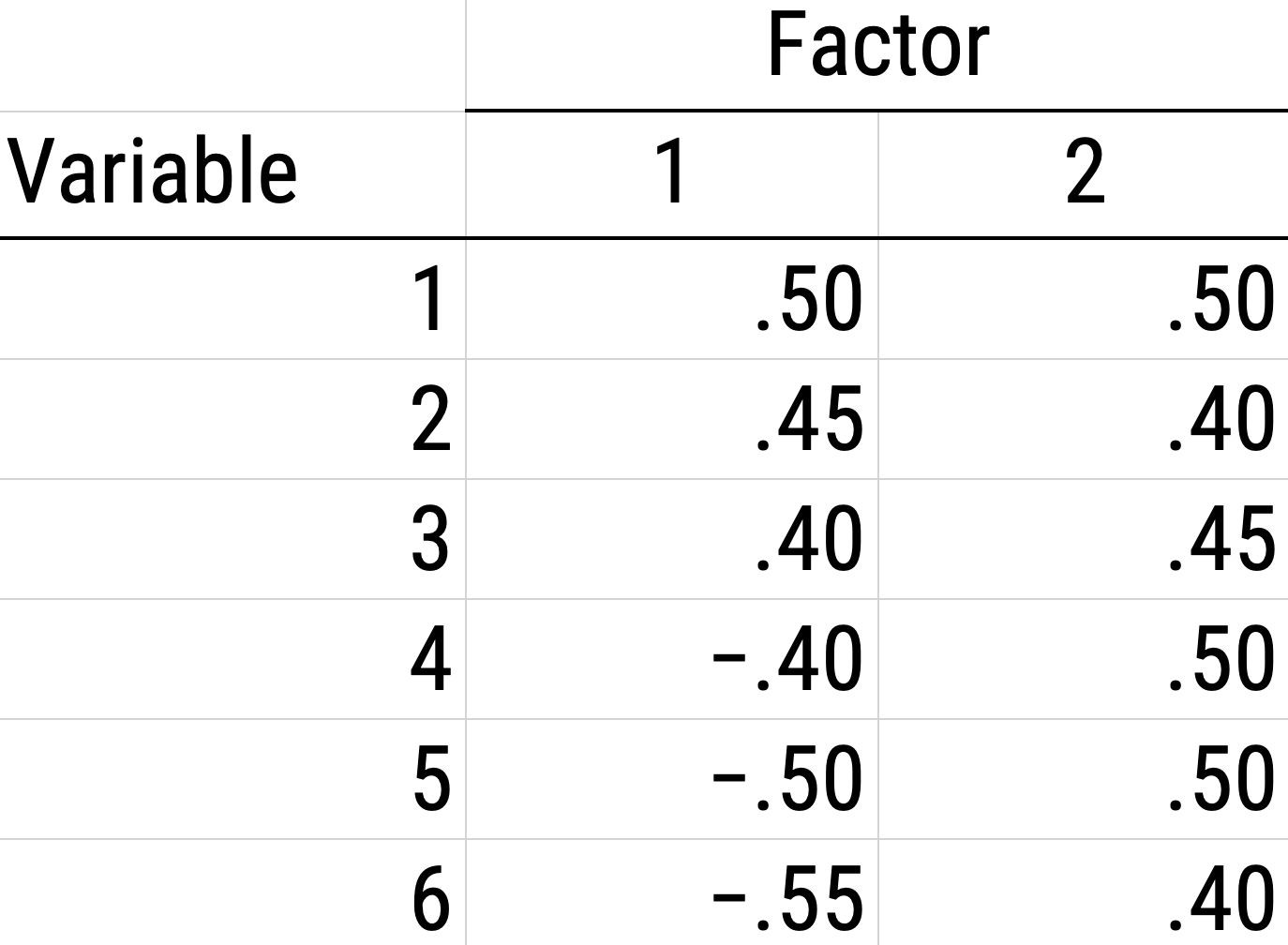
In the example factor matrix in Figure 22.5, the factor analysis is not very helpful—it tells us very little because it did not distinguish between the two factors. The variables have similar loadings on Factor 1 and Factor 2. An example of a unrotated factor solution is in Figure 22.5. In the figure, all of the variables are in the midst of the quadrants—they are not on the factors’ axes. Thus, the factors are not very informative.
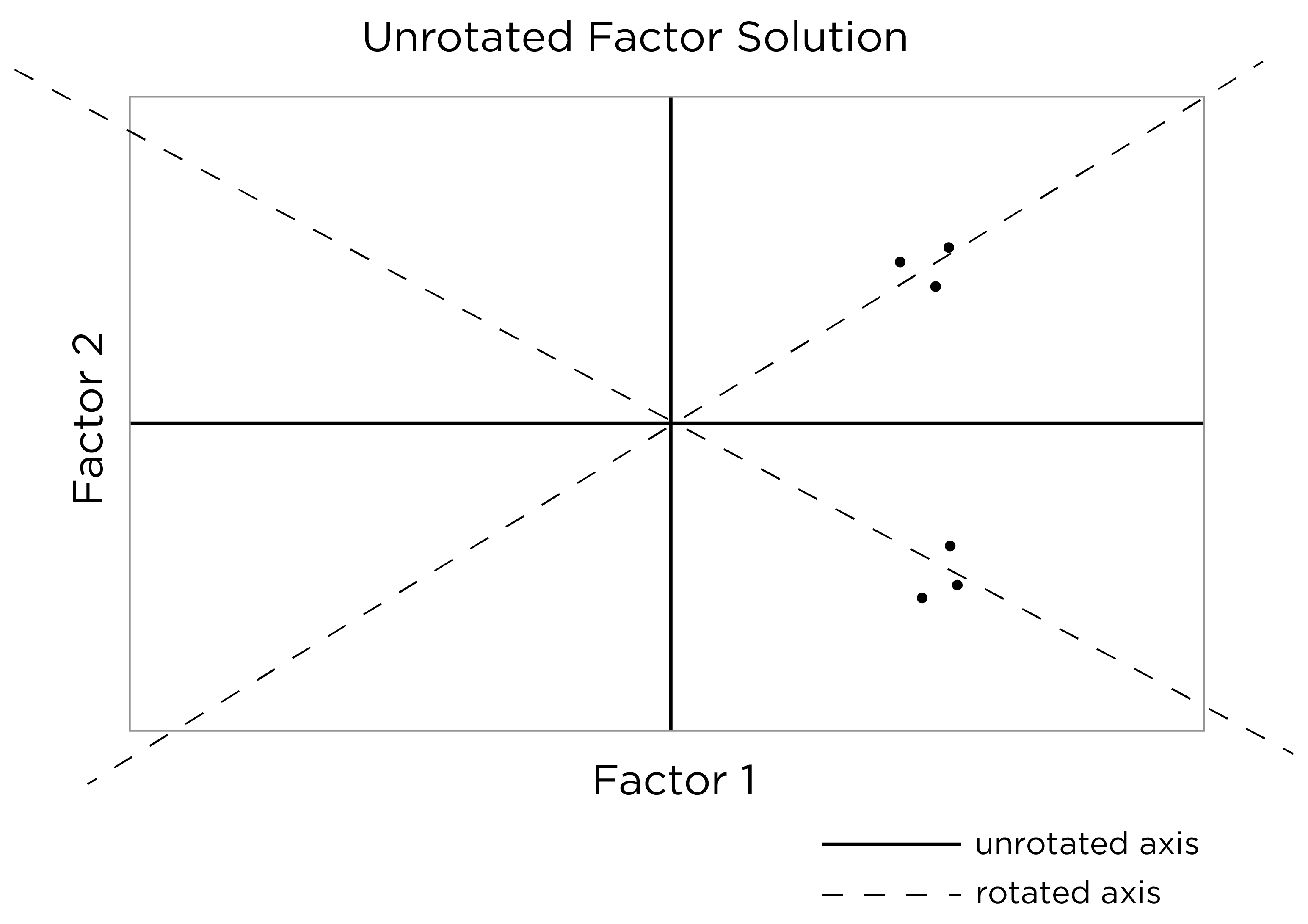
As a result, to improve the interpretability of the factor analysis, we can do what is called rotation. Rotation leverages the idea that there are infinite solutions to the factor analysis model that fit equally well. Rotation involves changing the orientation of the factors by changing the axes so that variables end up with very high (close to one or negative one) or very low (close to zero) loadings, so that it is clear which factors include which variables (and which factors each variable most strongly loads onto). That is, rotation rescales the factors and tries to identify the ideal solution (factor) for each variable. Rotation occurs by changing the variables’ loadings while keeping the structure of correlations among the variables intact (Field et al., 2012). Moreover, rotation does not change the variance explained by factors. Rotation searches for simple structure and keeps searching until it finds a minimum (i.e., the closest as possible to simple structure). After rotation, if the rotation was successful for imposing simple structure, each factor will have loadings close to one (or negative one) for some variables and close to zero for other variables. The goal of factor rotation is to achieve simple structure, to help make it easier to interpret the meaning of the factors.
To perform factor rotation, orthogonal rotations are often used. Orthogonal rotations make the rotated factors uncorrelated. An example of a commonly used orthogonal rotation is varimax rotation. Varimax rotation maximizes the sum of the variance of the squared loadings (i.e., so that items have either a very high or very low loading on a factor) and yields axes with a 90-degree angle.
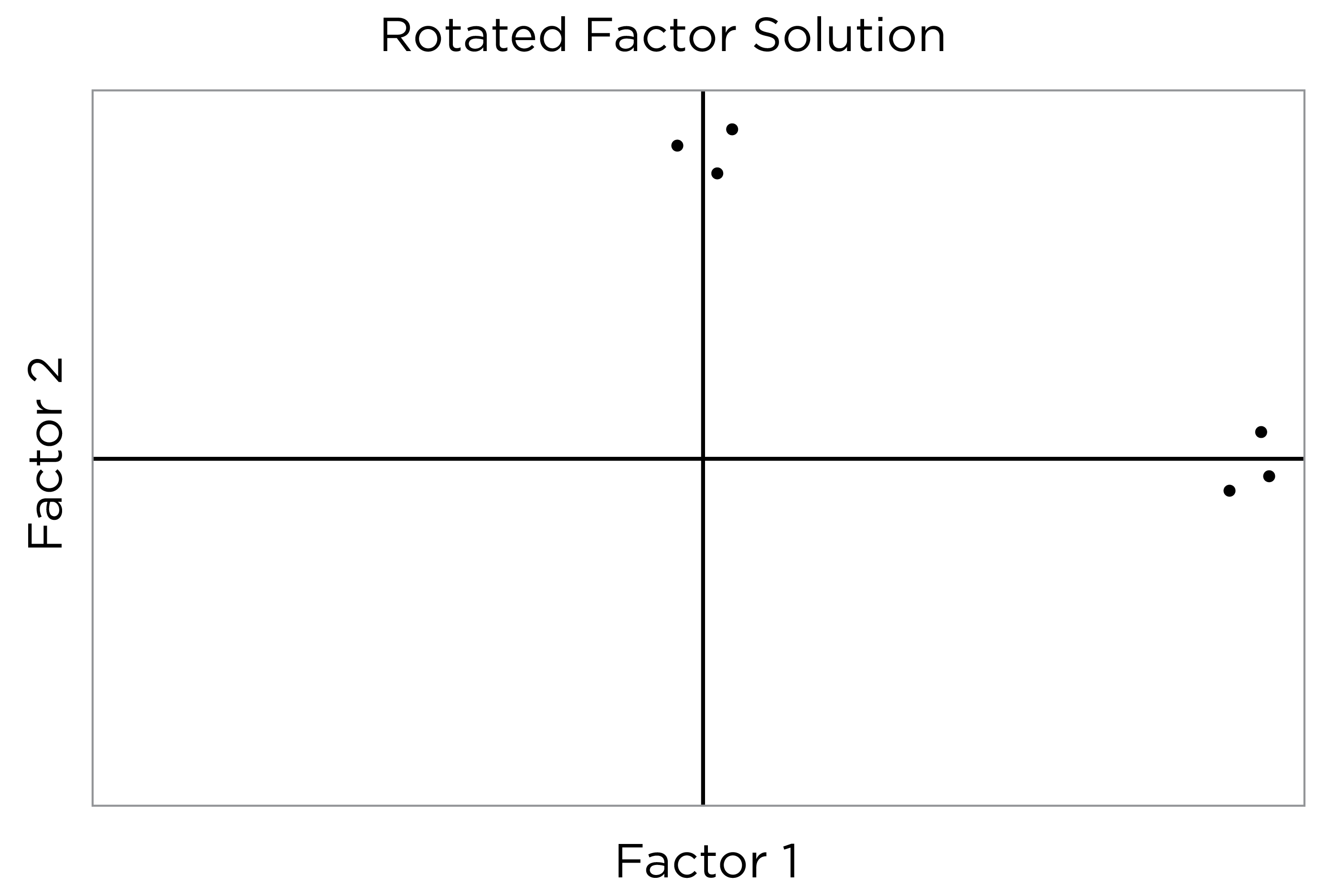
An example of a factor matrix following an orthogonal rotation is depicted in Figure 22.6. An example of a factor solution following an orthogonal rotation is depicted in Figure 22.7.
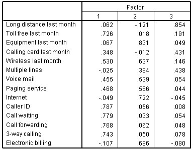
An example of a factor matrix from SPSS following an orthogonal rotation is depicted in Figure 22.8.
An example of a factor structure from an orthogonal rotation is in Figure 22.9.
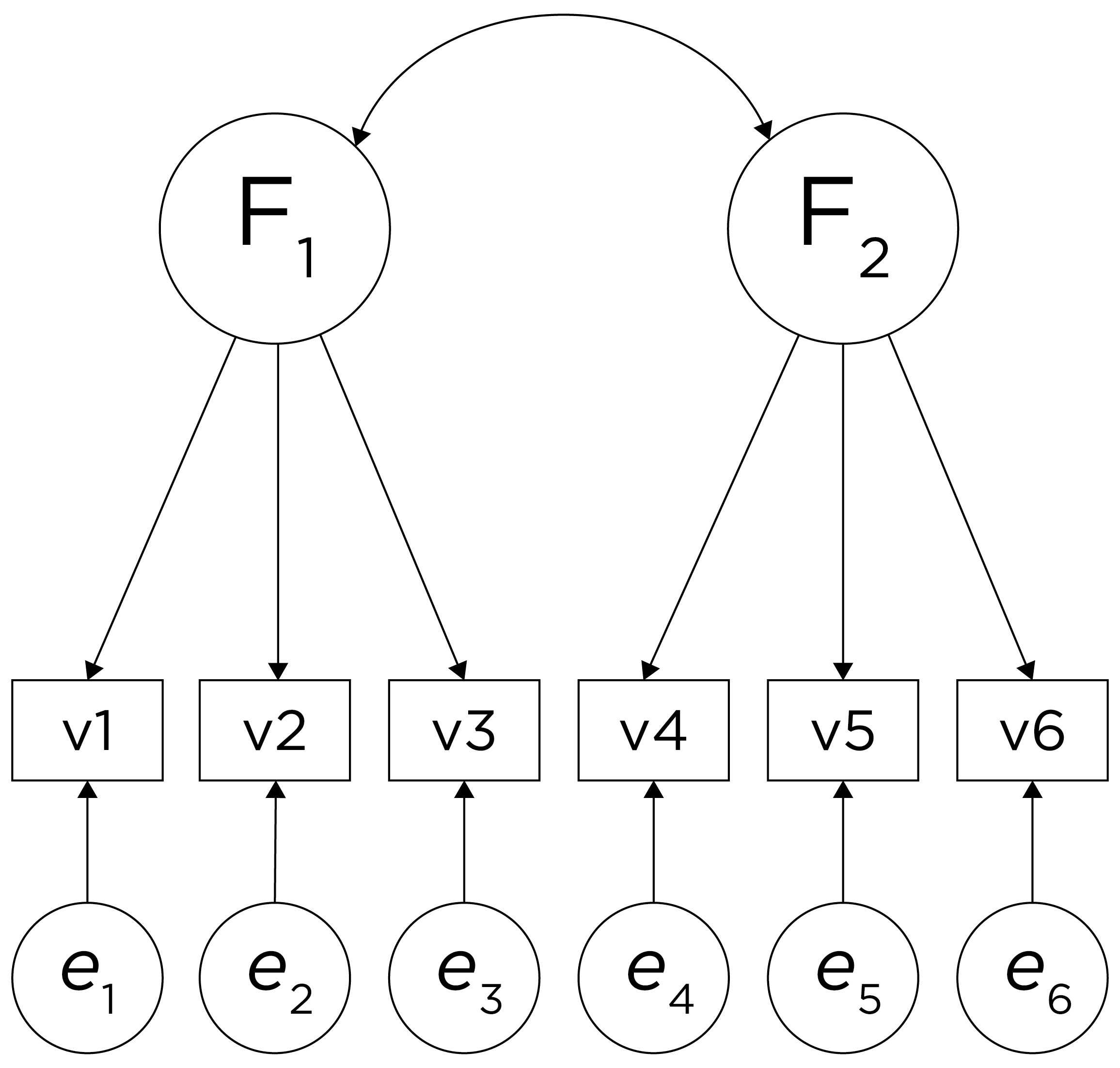
Sometimes, however, the two factors and their constituent variables may be correlated. Examples of two correlated factors may be depression and anxiety. When the two factors are correlated in reality, if we make them uncorrelated, this would result in an inaccurate model. Oblique rotation allows for factors to be correlated and yields axes with an angle of less than 90 degrees. However, if the factors have low correlation (e.g., .2 or less), you can likely continue with orthogonal rotation. Nevertheless, just because an oblique rotation allows for correlated factors does not mean that the factors will be correlated, so oblique rotation provides greater flexibility than orthogonal rotation. An example of a factor structure from an oblique rotation is in Figure 22.10. Results from an oblique rotation are more complicated than orthogonal rotation—they provide lots of output and are more complicated to interpret. In addition, oblique rotation might not yield a smooth answer if you have a relatively small sample size.
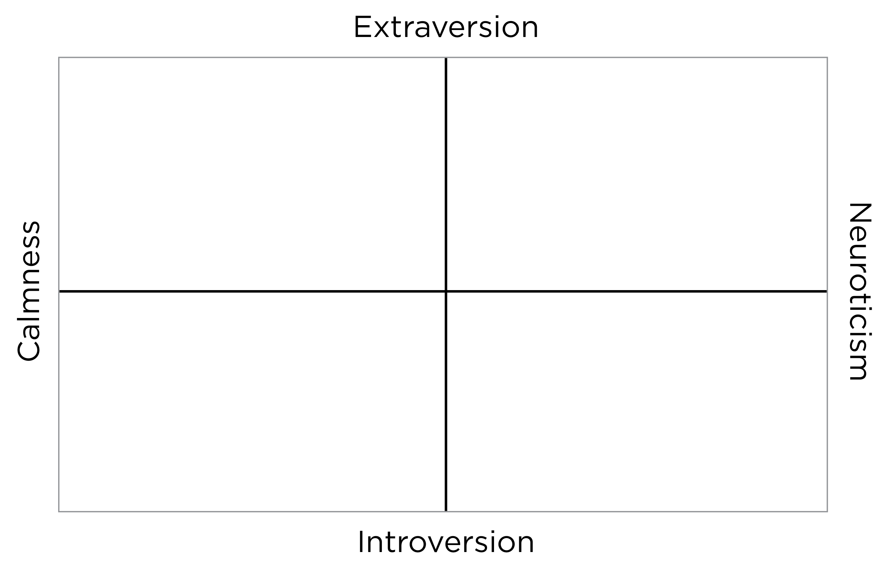
As an example of rotation based on interpretability, consider the Five-Factor Model of Personality (the Big Five), which goes by the acronym, OCEAN: Openness, Conscientiousness, Extraversion, Agreeableness, and Neuroticism. Although the five factors of personality are somewhat correlated, we can use rotation to ensure they are maximally independent. Upon rotation, extraversion and neuroticism are essentially uncorrelated, as depicted in Figure 22.11. The other pole of extraversion is intraversion and the other pole of neuroticism might be emotional stability or calmness.
Simple structure is achieved when each variable loads highly onto as few factors as possible (i.e., each item has only one significant or primary loading). Oftentimes this is not the case, so we choose our rotation method in order to decide if the factors can be correlated (an oblique rotation) or if the factors will be uncorrelated (an orthogonal rotation). If the factors are not correlated with each other, use an orthogonal rotation. The correlation between an item and a factor is a factor loading, which is simply a way to ask how much a variable is correlated with the underlying factor. However, its interpretation is more complicated if there are correlated factors!
An orthogonal rotation (e.g., varimax) can help with simplicity of interpretation because it seeks to yield simple structure without cross-loadings. Cross-loadings are instances where a variable loads onto multiple factors. My recommendation would always be to use an orthogonal rotation if you have reason to believe that finding simple structure in your data is possible; otherwise, the factors are extremely difficult to interpret—what exactly does a cross-loading even mean? However, you should always try an oblique rotation, too, to see how strongly the factors are correlated. Examples of oblique rotations include oblimin and promax.
22.5.4 4. Determining the Number of Factors to Retain
A goal of factor analysis and principal component analysis is simplification or parsimony, while still explaining as much variance as possible. The hope is that you can have fewer factors that explain the associations between the variables than the number of observed variables. It does not make sense to replace 18 variables with 18 latent factors because that would not result in any simplification. The fewer the number of factors retained, the greater the parsimony, but the greater the amount of information that is discarded (i.e., the less the variance accounted for in the variables). The more factors we retain, the less the amount of information that is discarded (i.e., more variance is accounted for in the variables), but the less the parsimony. But how do you decide on the number of factors?
There are a number of criteria that one can use to help determine how many factors/components to keep:
- Kaiser-Guttman criterion (Kaiser, 1960): factors with eigenvalues greater than zero
- or, for principal component analysis, components with eigenvalues greater than 1
- Cattell’s scree test (Cattell, 1966): the “elbow” (inflection point) in a scree plot minus one; sometimes operationalized with optimal coordinates (OC) or the acceleration factor (AF)
- Parallel analysis: factors that explain more variance than randomly simulated data
- Very simple structure (VSS) criterion: larger is better
- Velicer’s minimum average partial (MAP) test: smaller is better
- Akaike information criterion (AIC): smaller is better
- Bayesian information criterion (BIC): smaller is better
- Sample size-adjusted BIC (SABIC): smaller is better
- Root mean square error of approximation (RMSEA): smaller is better
- Chi-square difference test: smaller is better; a significant test indicates that the more complex model is significantly better fitting than the less complex model
- Standardized root mean square residual (SRMR): smaller is better
- Comparative Fit Index (CFI): larger is better
- Tucker Lewis Index (TLI): larger is better
There is not necessarily a “correct” criterion to use in determining how many factors to keep, so it is generally recommended that researchers use multiple criteria in combination with theory and interpretability.
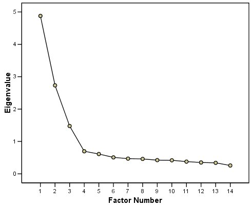
A scree plot provides lots of information. A scree plot has the factor number on the x-axis and the eigenvalue on the y-axis. The eigenvalue is the variance accounted for by a factor; when using a varimax (orthogonal) rotation, an eigenvalue (or factor variance) is calculated as the sum of squared standardized factor (or component) loadings on that factor. An example of a scree plot is in Figure 22.12.
The total variance is equal to the number of variables you have, so one eigenvalue is approximately one variable’s worth of variance. The first factor accounts for the most variance, the second factor accounts for the second-most variance, and so on. The more factors you add, the less variance is explained by the additional factor.
One criterion for how many factors to keep is the Kaiser-Guttman criterion. According to the Kaiser-Guttman criterion (Kaiser, 1960), you should keep any principal components (from PCA) whose eigenvalue is greater than 1 and factors (from factor analysis) whose eigenvalue is greater than 1. That is, for the sake of simplicity, parsimony, and data reduction, you should take any factors that explain more than a single variable would explain. According to the Kaiser-Guttman criterion, we would keep three components from Figure 22.12 that have eigenvalues greater than 1. The default in SPSS is to retain factors with eigenvalues greater than 1. However, keeping factors whose eigenvalue is greater than 1 is not the most correct rule. If you let SPSS do this, you may get many factors with eigenvalues around 1 (e.g., factors with an eigenvalue ~ 1.0001) that are not adding so much that it is worth the added complexity. The Kaiser-Guttman criterion usually results in keeping too many factors. Factors with small eigenvalues around 1 could reflect error shared across variables. For instance, factors with small eigenvalues could reflect method variance (i.e., method factor), such as a self-report factor that turns up as a factor in factor analysis, but that may be useless to you as a conceptual factor of a construct of interest.
Another criterion is Cattell’s scree test (Cattell, 1966), which involves selecting the number of factors from looking at the scree plot. “Scree” refers to the rubble of stones at the bottom of a mountain. According to Cattell’s scree test, you should keep the factors before the last steep drop in eigenvalues—i.e., the factors before the rubble, where the slope approaches zero. The beginning of the scree (or rubble), where the slope approaches zero, is called the “elbow” of a scree plot. Using Cattell’s scree test, you retain the number of factors that explain the most variance prior to the explained variance drop-off, because, ultimately, you want to include only as many factors in which you gain substantially more by the inclusion of these factors. That is, you would keep the number of factors at the elbow of the scree plot minus one. If the last steep drop occurs from Factor 4 to Factor 5 and the elbow is at Factor 5, we would keep four factors. In Figure 22.12, the last steep drop in eigenvalues occurs from Factor 3 to Factor 4; the elbow of the scree plot occurs at Factor 4. We would keep the number of factors at the elbow minus one. Thus, using Cattell’s scree test, we would keep three factors based on Figure 22.12.
There are more sophisticated ways of using a scree plot, but they usually end up at a similar decision. Examples of more sophisticated tests include parallel analysis and very simple structure (VSS) plots. In a parallel analysis, you examine where the eigenvalues from observed data and random data converge, so you do not retain a factor that explains less variance than would be expected by random chance. Using the VSS criterion, the optimal number of factors to retain is the number of factors that maximizes the VSS criterion (Revelle & Rocklin, 1979). The VSS criterion is evaluated with models in which factor loadings for a given item that are less than the maximum factor loading for that item are suppressed to zero, thus forcing simple structure (i.e., no cross-loadings). The goal is finding a factor structure with interpretability so that factors are clearly distinguishable. Thus, we want to identify the number of factors with the highest VSS criterion.
In general, my recommendation is to use Cattell’s scree test, and then test the factor solutions with plus or minus one factor, in addition to examining model fit. You should never accept factors with eigenvalues less than zero (or components from PCA with eigenvalues less than one), because they are likely to be largely composed of error. If you are using maximum likelihood factor analysis, you can compare the fit of various models with model fit criteria to see which model fits best for its parsimony. A model will always fit better when you add additional parameters or factors, so you examine if there is significant improvement in model fit when adding the additional factor—that is, we keep adding complexity until additional complexity does not buy us much. Always try a factor solution that is one less and one more than suggested by Cattell’s scree test to buffer your final solution because the purpose of factor analysis is to explain things and to have interpretability. Even if all rules or indicators suggest to keep X number of factors, maybe \(\pm\) one factor helps clarify things. Even though factor analysis is empirical, theory and interpretatability should also inform decisions.
22.5.4.1 Model Fit Indices
In factor analysis, we fit a model to observed data, or to the variance-covariance matrix, and we evaluate the degree of model misfit. That is, fit indices evaluate how likely it is that a given causal model gave rise to the observed data. Various model fit indices can be used for evaluating how well a model fits the data and for comparing the fit of two competing models. Fit indices known as absolute fit indices compare whether the model fits better than the best-possible fitting model (i.e., a saturated model). Examples of absolute fit indices include the chi-square test, root mean square error of approximation (RMSEA), and the standardized root mean square residual (SRMR).
The chi-square test evaluates whether the model has a significant degree of misfit relative to the best-possible fitting model (a saturated model that fits as many parameters as possible; i.e., as many parameters as there are degrees of freedom); the null hypothesis of a chi-square test is that there is no difference between the predicted data (i.e., the data that would be observed if the model were true) and the observed data. Thus, a non-significant chi-square test indicates good model fit. However, because the null hypothesis of the chi-square test is that the model-implied covariance matrix is exactly equal to the observed covariance matrix (i.e., a model of perfect fit), this may be an unrealistic comparison. Models are simplifications of reality, and our models are virtually never expected to be a perfect description of reality. Thus, we would say a model is “useful” and partially validated if “it helps us to understand the relation between variables and does a ‘reasonable’ job of matching the data…A perfect fit may be an inappropriate standard, and a high chi-square estimate may indicate what we already know—that the hypothesized model holds approximately, not perfectly.” (Bollen, 1989, p. 268). The power of the chi-square test depends on sample size, and a large sample will likely detect small differences as significantly worse than the best-possible fitting model (Bollen, 1989).
RMSEA is an index of absolute fit. Lower values indicate better fit.
SRMR is an index of absolute fit with no penalty for model complexity. Lower values indicate better fit.
There are also various fit indices known as incremental, comparative, or relative fit indices that compare whether the model fits better than the worst-possible fitting model (i.e., a “baseline” or “null” model). Incremental fit indices include a chi-square difference test, the comparative fit index (CFI), and the Tucker-Lewis index (TLI). Unlike the chi-square test comparing the model to the best-possible fitting model, a significant chi-square test of the relative fit index indicates better fit—i.e., that the model fits better than the worst-possible fitting model.
CFI is another relative fit index that compares the model to the worst-possible fitting model. Higher values indicate better fit.
TLI is another relative fit index. Higher values indicate better fit.
Parsimony fit include fit indices that use information criteria fit indices, including the Akaike Information Criterion (AIC) and the Bayesian Information Criterion (BIC). BIC penalizes model complexity more so than AIC. Lower AIC and BIC values indicate better fit.
Chi-square difference tests and CFI can be used to compare two nested models. AIC and BIC can be used to compare two non-nested models.
Criteria for acceptable fit and good fit of SEM models are in Table 22.1. In addition, dynamic fit indexes have been proposed based on simulation to identify fit index cutoffs that are tailored to the characteristics of the specific model and data (McNeish & Wolf, 2023); dynamic fit indexes are available via the dynamic package (Wolf & McNeish, 2022) or with a webapp.
| SEM Fit Index | Acceptable Fit | Good Fit |
|---|---|---|
| RMSEA | \(\leq\) .08 | \(\leq\) .05 |
| CFI | \(\geq\) .90 | \(\geq\) .95 |
| TLI | \(\geq\) .90 | \(\geq\) .95 |
| SRMR | \(\leq\) .10 | \(\leq\) .08 |
However, good model fit does not necessarily indicate a true model.
In addition to global fit indices, it can also be helpful to examine evidence of local fit, such as the residual covariance matrix. The residual covariance matrix represents the difference between the observed covariance matrix and the model-implied covariance matrix (the observed covariance matrix minus the model-implied covariance matrix). These difference values are called covariance residuals. Standardizing the covariance matrix by converting each to a correlation matrix can be helpful for interpreting the magnitude of any local misfit. This is known as a residual correlation matrix, which is composed of correlation residuals. Correlation residuals greater than |.10| are possible evidence for poor local fit (Kline, 2023). If a correlation residual is positive, it suggests that the model underpredicts the observed association between the two variables (i.e., the observed covariance is greater than the model-implied covariance). If a correlation residual is negative, it suggests that the model overpredicts their observed association between the two variables (i.e., the observed covariance is smaller than the model-implied covariance). If the two variables are connected by only indirect pathways, it may be helpful to respecify the model with direct pathways between the two variables, such as a direct effect (i.e., regression path) or a covariance path. For guidance on evaluating local fit, see Kline (2024).
22.5.5 5. Interpreting and Using Latent Factors
The next step is interpreting the model and latent factors. One data matrix can lead to many different (correct) models—you must choose one based on the factor structure and theory. Use theory to interpret the model and label the factors. In latent variable models, factors have meaning. You can use them as predictors, mediators, moderators, or outcomes. When possible, it is preferable to use the factors by examining their associations with other variables in the same model. You can extract factor scores, if necessary, for use in other analyses; however, it is preferable to examine the associations between factors and other variables in the same model if possible. And, using latent factors helps disattenuate associations for measurement error, to identify what the association is between variables when removing random measurement error.
22.6 Example of Exploratory Factor Analysis
We generated the scree plot in Figure 22.13 using the psych::fa.parallel() function of the psych package (Revelle, 2025). The optimal coordinates and the acceleration factor attempt to operationalize the Cattell scree test: i.e., the “elbow” of the scree plot (Ruscio & Roche, 2012). The optimal coordinators factor is quantified using a series of linear equations to determine whether observed eigenvalues exceed the predicted values. The acceleration factor is quantified using the acceleration of the curve, that is, the second derivative. The Kaiser-Guttman rule states to keep principal components whose eigenvalues are greater than 1. However, for exploratory factor analysis (as opposed to PCA), the criterion is to keep the factors whose eigenvalues are greater than zero (i.e., not the factors whose eigenvalues are greater than 1) (Dinno, 2014).
The number of factors to keep would depend on which criteria one uses. Based on the rule to keep factors whose eigenvalues are greater than zero and based on the parallel test, we would keep five factors. However, based on the Cattell scree test (the “elbow” of the screen plot minus one), we would keep three factors. If using the optimal coordinates, we would keep eight factors; if using the acceleration factor, we would keep one factor. Therefore, interpretability of the factors would be important for deciding how many factors to keep.
Code
Parallel analysis suggests that the number of factors = 5 and the number of components = NA 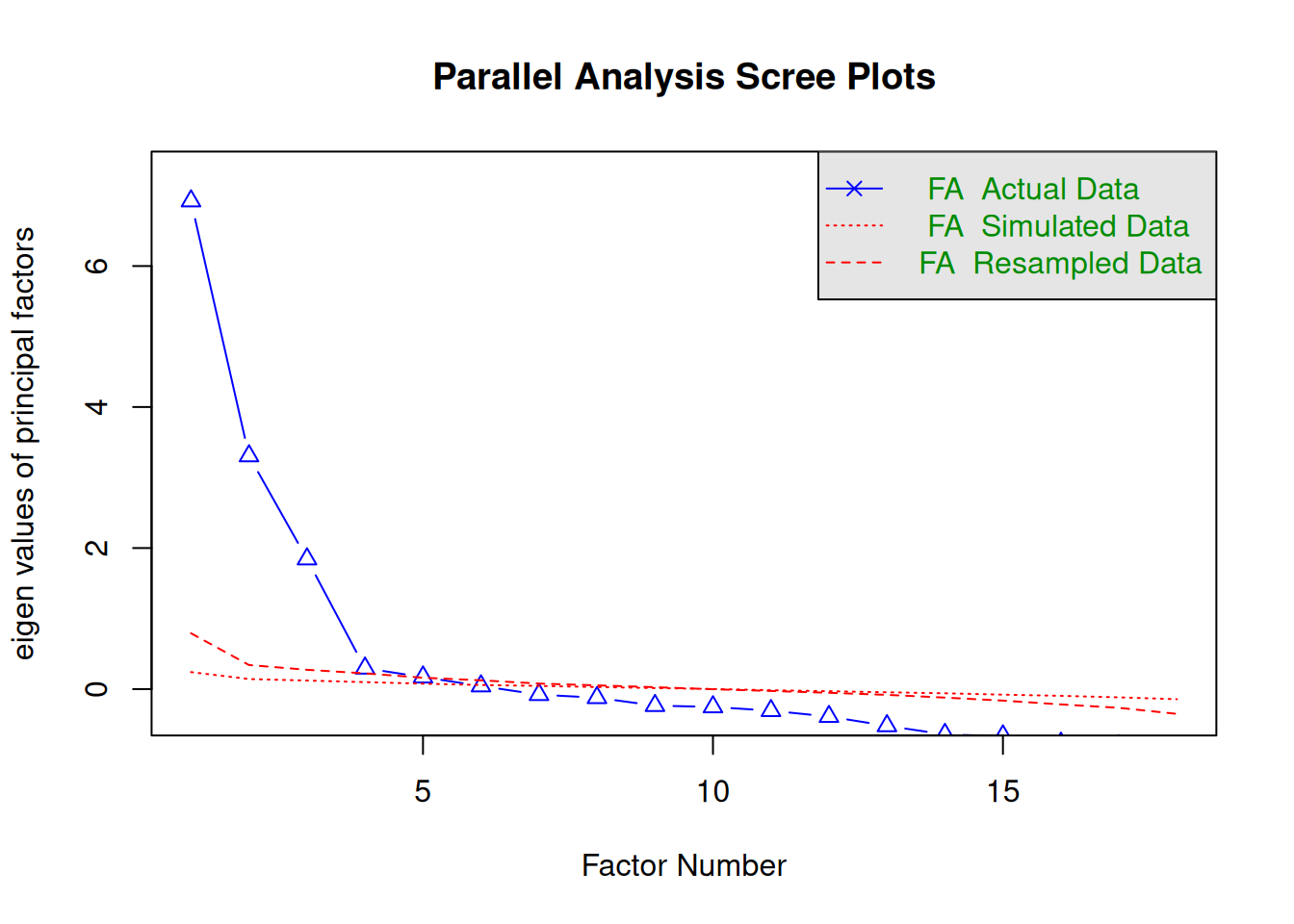
We generated the scree plot in Figure 22.14 using the nFactors::nScree() and nFactors::plotnScree() functions of the nFactors package (Raiche & Magis, 2025).
Code
#screeDataEFA <- nFactors::nScree(
#  x = cor( # throws error with correlation matrix, so use covariance instead (below)
#    dataForFA[faVars],
#    use = "pairwise.complete.obs"),
#  model = "factors")

screeDataEFA <- nFactors::nScree(
  x = cov(
    dataForFA[faVars],
    use = "pairwise.complete.obs"),
  cor = FALSE,
  model = "factors")

nFactors::plotnScree(screeDataEFA)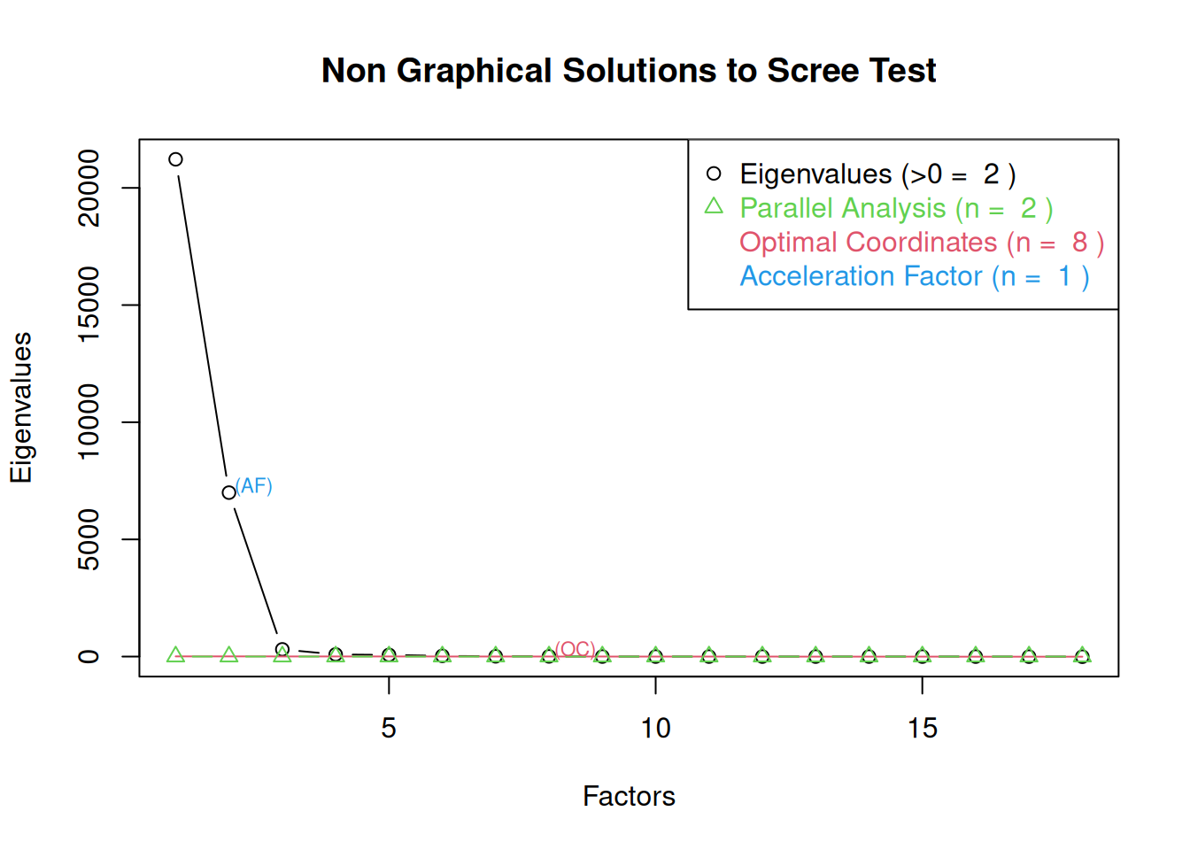
We generated the very simple structure (VSS) plots in Figures 22.15 and 22.16 using the psych::vss() and psych::nfactors() functions of the psych package (Revelle, 2025). In addition to VSS plots, the output also provides additional criteria by which to determine the optimal number of factors, each for which lower values are better, including the Velicer minimum average partial (MAP) test, the Bayesian information criterion (BIC), the sample size-adjusted BIC (SABIC), and the root mean square error of approximation (RMSEA). Depending on the criterion, the optimal number of factors extracted varies between 2 and 8 factors.
Very Simple Structure
Call: psych::vss(x = dataForFA[faVars], rotate = "oblimin", fm = "minres")
VSS complexity 1 achieves a maximimum of 0.78  with  2  factors
VSS complexity 2 achieves a maximimum of 0.87  with  3  factors

The Velicer MAP achieves a minimum of 0.13  with  3  factors
BIC achieves a minimum of  -177286.1  with  7  factors
Sample Size adjusted BIC achieves a minimum of  -177133.6  with  7  factors

Statistics by number of factors
  vss1 vss2  map dof  chisq prob sqresid  fit RMSEA     BIC   SABIC complex
1 0.68 0.00 0.19 135 158630    0    25.6 0.68  0.75  157598  158027     1.0
2 0.78 0.86 0.16 118 144322    0    11.2 0.86  0.76  143420  143795     1.2
3 0.77 0.87 0.13 102    NaN  NaN     9.1 0.89    NA      NA      NA     1.2
4 0.77 0.86 0.15  87 135998    0     8.3 0.90  0.86  135332  135609     1.3
5 0.72 0.81 0.30  73 150332    0    10.7 0.87  0.99  149774  150006     1.4
6 0.63 0.78 0.41  60    NaN  NaN    13.3 0.84    NA      NA      NA     1.4
7 0.64 0.75 4.73  48      0    1    12.9 0.84  0.00 -177286 -177134     1.6
8 0.53 0.69  NaN  37 117148    0    18.1 0.78  1.23  116865  116983     1.5
  eChisq   SRMR eCRMS  eBIC
1  18286 0.1690 0.180 17254
2   5646 0.0939 0.107  4744
3    814 0.0357 0.044    35
4    476 0.0273 0.036  -190
5    246 0.0196 0.028  -312
6    128 0.0141 0.023  -331
7     69 0.0104 0.019  -298
8     21 0.0058 0.012  -261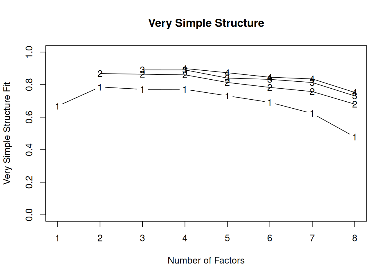
Code
Number of factors
Call: vss(x = x, n = n, rotate = rotate, diagonal = diagonal, fm = fm,
    n.obs = n.obs, plot = FALSE, title = title, use = use, cor = cor)
VSS complexity 1 achieves a maximimum of 0.78  with  2  factors
VSS complexity 2 achieves a maximimum of 0.87  with  3  factors
The Velicer MAP achieves a minimum of 0.13  with  3  factors
Empirical BIC achieves a minimum of  -331.09  with  6  factors
Sample Size adjusted BIC achieves a minimum of  -177133.7  with  7  factors

Statistics by number of factors
   vss1 vss2  map dof  chisq prob sqresid  fit RMSEA     BIC   SABIC complex
1  0.68 0.00 0.19 135 158630    0    25.6 0.68  0.75  157598  158027     1.0
2  0.78 0.86 0.16 118 144322    0    11.2 0.86  0.76  143420  143795     1.2
3  0.77 0.87 0.13 102    NaN  NaN     9.1 0.89    NA      NA      NA     1.2
4  0.77 0.86 0.15  87 135998    0     8.3 0.90  0.86  135332  135609     1.3
5  0.72 0.81 0.30  73 150332    0    10.7 0.87  0.99  149774  150006     1.4
6  0.63 0.78 0.41  60    NaN  NaN    13.3 0.84    NA      NA      NA     1.4
7  0.64 0.75 4.73  48      0    1    12.9 0.84  0.00 -177286 -177134     1.6
8  0.53 0.69  NaN  37 117148    0    18.1 0.78  1.23  116865  116983     1.5
9  0.53 0.67  NaN  27 110830    0    19.3 0.76  1.40  110624  110709     1.5
10 0.33 0.49  NaN  18 175145    0    28.7 0.64  2.16  175008  175065     1.8
11 0.30 0.41  NaN  10    NaN  NaN    32.2 0.60    NA      NA      NA     2.1
12 0.25 0.39  NaN   3    NaN  NaN    35.3 0.56    NA      NA      NA     2.2
13 0.24 0.34  NaN  -3  59960   NA    40.0 0.51    NA      NA      NA     2.1
14 0.23 0.30  NaN  -8  62025   NA    42.3 0.48    NA      NA      NA     2.3
15 0.20 0.27  NaN -12    NaN   NA    45.4 0.44    NA      NA      NA     2.3
16 0.22 0.27  NaN -15    NaN   NA    45.0 0.44    NA      NA      NA     2.7
17 0.18 0.23  NaN -17    NaN   NA    49.4 0.39    NA      NA      NA     2.4
18 0.40 0.46   NA -18    NaN   NA    35.4 0.56    NA      NA      NA     2.0
    eChisq   SRMR eCRMS  eBIC
1  18286.4 0.1690 0.180 17254
2   5645.9 0.0939 0.107  4744
3    814.5 0.0357 0.044    35
4    475.7 0.0273 0.036  -190
5    246.2 0.0196 0.028  -312
6    127.7 0.0141 0.023  -331
7     69.0 0.0104 0.019  -298
8     21.5 0.0058 0.012  -261
9     13.0 0.0045 0.011  -193
10     9.7 0.0039 0.011  -128
11     8.1 0.0036 0.014   -68
12     6.3 0.0031 0.022   -17
13     5.3 0.0029    NA    NA
14     5.0 0.0028    NA    NA
15     5.0 0.0028    NA    NA
16     5.0 0.0028    NA    NA
17     5.0 0.0028    NA    NA
18     5.0 0.0028    NA    NA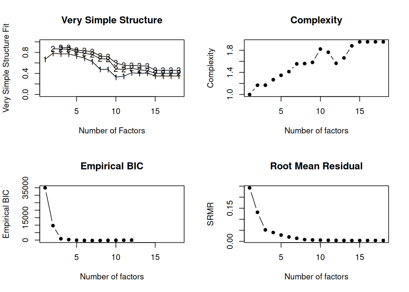
We fit EFA models using the lavaan::efa() function of the lavaan package (Rosseel, 2012; Rosseel et al., 2024).
The model fits well according to CFI with 5 or more factors; the model fits well according to RMSEA with 6 or more factors. However, 5+ factors does not represent much of a simplification (relative to the 18 variables included). Moreover, in the model with four factors, only one variable had a significant loading on Factor 1. Thus, even with four factors, one of the factors does not seem to represent the aggregation of multiple variables. For these reasons, and because the “elbow test” for the scree plot suggested three factors, we decided to retain three factors and to see if we could achieve better fit by making additional model modifications (e.g., correlated residuals). Correlated residuals may be necessary, for example, when variables are correlated for reasons other than the latent factors.
This is lavaan 0.6-21 -- running exploratory factor analysis
Estimator ML
Rotation method GEOMIN OBLIQUE
Geomin epsilon 0.001
Rotation algorithm (rstarts) GPA (30)
Standardized metric TRUE
Row weights None
Number of observations 2093
Number of missing patterns 5
Overview models:
aic bic sabic chisq df pvalue cfi rmsea
nfactors = 1 146817.6 147122.5 146951.0 18696.759 135 0 0.042 0.617
nfactors = 2 125003.9 125404.8 125179.2 5413.526 118 0 0.669 0.392
nfactors = 3 120616.6 121107.8 120831.4 3225.455 102 0 0.743 0.380
nfactors = 4 117389.2 117965.2 117641.1 1482.963 87 0 0.890 0.286
nfactors = 5 116253.8 116908.8 116540.2 749.654 73 0 0.917 0.308
nfactors = 6 115897.4 116625.8 116216.0 536.174 60 0 0.943 0.385
nfactors = 7 115598.8 116394.9 115947.0 1815.516 48 0 1.000 0.720
Eigenvalues correlation matrix:
ev1 ev2 ev3 ev4 ev5 ev6 ev7 ev8
7.03951 6.25329 2.83858 0.52506 0.39207 0.32686 0.20711 0.10947
ev9 ev10 ev11 ev12 ev13 ev14 ev15 ev16
0.08752 0.06111 0.04277 0.03547 0.02461 0.02112 0.01725 0.00965
ev17 ev18
0.00659 0.00194
Number of factors: 1
Standardized loadings: (* = significant at 1% level)
f1 unique.var communalities
completionsPerGame 0.885* 0.216 0.784
attemptsPerGame 0.885* 0.216 0.784
passing_yardsPerGame 0.875* 0.234 0.766
passing_tdsPerGame 0.741* 0.450 0.550
passing_air_yardsPerGame 0.587* 0.655 0.345
passing_yards_after_catchPerGame 0.726* 0.472 0.528
passing_first_downsPerGame 0.870* 0.243 0.757
avg_completed_air_yards -0.987* 0.026 0.974
avg_intended_air_yards -0.999* 0.002 0.998
aggressiveness -0.889* 0.210 0.790
max_completed_air_distance -0.936* 0.123 0.877
avg_air_distance -0.994* 0.012 0.988
max_air_distance -0.942* 0.112 0.888
avg_air_yards_to_sticks -0.997* 0.006 0.994
passing_cpoe .* 0.916 0.084
pass_comp_pct .* 0.913 0.087
passer_rating -0.532* 0.717 0.283
completion_percentage_above_expectation -0.568* 0.677 0.323
f1
Sum of squared loadings 11.798
Proportion of total 1.000
Proportion var 0.655
Cumulative var 0.655
Number of factors: 2
Standardized loadings: (* = significant at 1% level)
f1 f2 unique.var
completionsPerGame 0.985* 0.029
attemptsPerGame 0.974* * 0.050
passing_yardsPerGame 0.996* 0.008
passing_tdsPerGame 0.867* 0.249
passing_air_yardsPerGame 0.721* 0.685* 0.034
passing_yards_after_catchPerGame 0.763* -0.605* 0.029
passing_first_downsPerGame 0.990* 0.019
avg_completed_air_yards 0.967* 0.065
avg_intended_air_yards * 0.998* 0.002
aggressiveness .* 0.771* 0.388
max_completed_air_distance .* 0.818* 0.271
avg_air_distance * 0.979* 0.032
max_air_distance .* 0.856* 0.245
avg_air_yards_to_sticks 0.992* 0.016
passing_cpoe 0.327* -0.304* 0.796
pass_comp_pct .* 0.916
passer_rating 0.597* . 0.621
completion_percentage_above_expectation 0.460* . 0.733
communalities
completionsPerGame 0.971
attemptsPerGame 0.950
passing_yardsPerGame 0.992
passing_tdsPerGame 0.751
passing_air_yardsPerGame 0.966
passing_yards_after_catchPerGame 0.971
passing_first_downsPerGame 0.981
avg_completed_air_yards 0.935
avg_intended_air_yards 0.998
aggressiveness 0.612
max_completed_air_distance 0.729
avg_air_distance 0.968
max_air_distance 0.755
avg_air_yards_to_sticks 0.984
passing_cpoe 0.204
pass_comp_pct 0.084
passer_rating 0.379
completion_percentage_above_expectation 0.267
f2 f1 total
Sum of sq (obliq) loadings 6.879 6.619 13.497
Proportion of total 0.510 0.490 1.000
Proportion var 0.382 0.368 0.750
Cumulative var 0.382 0.750 0.750
Factor correlations: (* = significant at 1% level)
f1 f2
f1 1.000
f2 -0.024 1.000
Number of factors: 3
Standardized loadings: (* = significant at 1% level)
f1 f2 f3 unique.var
completionsPerGame 0.978* * 0.026
attemptsPerGame 0.993* * * 0.039
passing_yardsPerGame 0.987* * 0.010
passing_tdsPerGame 0.837* * .* 0.251
passing_air_yardsPerGame 0.787* 0.719* 0.023
passing_yards_after_catchPerGame 0.714* -0.593* 0.031
passing_first_downsPerGame 0.979* * 0.020
avg_completed_air_yards 0.774* 0.349* 0.039
avg_intended_air_yards 0.882* .* 0.002
aggressiveness 0.793* 0.375
max_completed_air_distance .* 0.667* 0.371* 0.175
avg_air_distance * 0.876* .* 0.025
max_air_distance .* 0.815* . 0.208
avg_air_yards_to_sticks 0.860* .* 0.012
passing_cpoe 1.001* 0.022
pass_comp_pct -0.473* 1.056* 0.104
passer_rating * 0.926* 0.090
completion_percentage_above_expectation 0.964* 0.045
communalities
completionsPerGame 0.974
attemptsPerGame 0.961
passing_yardsPerGame 0.990
passing_tdsPerGame 0.749
passing_air_yardsPerGame 0.977
passing_yards_after_catchPerGame 0.969
passing_first_downsPerGame 0.980
avg_completed_air_yards 0.961
avg_intended_air_yards 0.998
aggressiveness 0.625
max_completed_air_distance 0.825
avg_air_distance 0.975
max_air_distance 0.792
avg_air_yards_to_sticks 0.988
passing_cpoe 0.978
pass_comp_pct 0.896
passer_rating 0.910
completion_percentage_above_expectation 0.955
f2 f1 f3 total
Sum of sq (obliq) loadings 5.997 5.788 4.720 16.504
Proportion of total 0.363 0.351 0.286 1.000
Proportion var 0.333 0.322 0.262 0.917
Cumulative var 0.333 0.655 0.917 0.917
Factor correlations: (* = significant at 1% level)
f1 f2 f3
f1 1.000
f2 -0.128* 1.000
f3 0.168* 0.446* 1.000
Number of factors: 4
Standardized loadings: (* = significant at 1% level)
f1 f2 f3 f4
completionsPerGame 0.972* *
attemptsPerGame * 1.027*
passing_yardsPerGame .* 0.900*
passing_tdsPerGame 0.377* 0.669*
passing_air_yardsPerGame 0.816* 0.723*
passing_yards_after_catchPerGame .* 0.616* -0.599*
passing_first_downsPerGame .* 0.902* *
avg_completed_air_yards .* 0.953*
avg_intended_air_yards 1.019*
aggressiveness 0.813*
max_completed_air_distance .* .* 0.780*
avg_air_distance 0.997*
max_air_distance .* 0.876*
avg_air_yards_to_sticks 1.000*
passing_cpoe . 0.920*
pass_comp_pct -0.450* 1.070*
passer_rating .* 0.801*
completion_percentage_above_expectation . 0.892*
unique.var communalities
completionsPerGame 0.015 0.985
attemptsPerGame 0.001 0.999
passing_yardsPerGame 0.000 1.000
passing_tdsPerGame 0.203 0.797
passing_air_yardsPerGame 0.016 0.984
passing_yards_after_catchPerGame 0.024 0.976
passing_first_downsPerGame 0.023 0.977
avg_completed_air_yards 0.061 0.939
avg_intended_air_yards 0.003 0.997
aggressiveness 0.345 0.655
max_completed_air_distance 0.271 0.729
avg_air_distance 0.034 0.966
max_air_distance 0.219 0.781
avg_air_yards_to_sticks 0.017 0.983
passing_cpoe 0.037 0.963
pass_comp_pct 0.074 0.926
passer_rating 0.146 0.854
completion_percentage_above_expectation 0.029 0.971
f3 f2 f4 f1 total
Sum of sq (obliq) loadings 6.929 5.410 3.431 0.714 16.483
Proportion of total 0.420 0.328 0.208 0.043 1.000
Proportion var 0.385 0.301 0.191 0.040 0.916
Cumulative var 0.385 0.685 0.876 0.916 0.916
Factor correlations: (* = significant at 1% level)
f1 f2 f3 f4
f1 1.000
f2 0.402* 1.000
f3 0.010 -0.154* 1.000
f4 0.310* 0.137* 0.441* 1.000
Number of factors: 5
Standardized loadings: (* = significant at 1% level)
f1 f2 f3 f4 f5
completionsPerGame 0.949* * .*
attemptsPerGame 0.972* *
passing_yardsPerGame 0.854* .*
passing_tdsPerGame 0.644* 0.436*
passing_air_yardsPerGame 0.796* 0.745* *
passing_yards_after_catchPerGame 0.526* 0.306* -0.595* .* *
passing_first_downsPerGame 0.870* .* *
avg_completed_air_yards 0.989* .*
avg_intended_air_yards 1.001*
aggressiveness . 0.781* .
max_completed_air_distance .* . 0.724*
avg_air_distance 0.951* .*
max_air_distance .* 0.678* .* .
avg_air_yards_to_sticks 0.974*
passing_cpoe . 0.897*
pass_comp_pct .* 1.037*
passer_rating 0.316* 0.758*
completion_percentage_above_expectation .* 0.852*
unique.var communalities
completionsPerGame 0.008 0.992
attemptsPerGame 0.005 0.995
passing_yardsPerGame 0.003 0.997
passing_tdsPerGame 0.186 0.814
passing_air_yardsPerGame 0.016 0.984
passing_yards_after_catchPerGame 0.000 1.000
passing_first_downsPerGame 0.018 0.982
avg_completed_air_yards 0.039 0.961
avg_intended_air_yards 0.002 0.998
aggressiveness 0.456 0.544
max_completed_air_distance 0.326 0.674
avg_air_distance 0.050 0.950
max_air_distance 0.280 0.720
avg_air_yards_to_sticks 0.026 0.974
passing_cpoe 0.020 0.980
pass_comp_pct 0.096 0.904
passer_rating 0.139 0.861
completion_percentage_above_expectation 0.039 0.961
f3 f1 f5 f2 f4 total
Sum of sq (obliq) loadings 6.451 5.148 3.379 1.031 0.281 16.291
Proportion of total 0.396 0.316 0.207 0.063 0.017 1.000
Proportion var 0.358 0.286 0.188 0.057 0.016 0.905
Cumulative var 0.358 0.644 0.832 0.889 0.905 0.905
Factor correlations: (* = significant at 1% level)
f1 f2 f3 f4 f5
f1 1.000
f2 0.404* 1.000
f3 -0.093 0.086 1.000
f4 0.229* 0.136 0.004 1.000
f5 0.136* 0.392* 0.445* 0.279 1.000
Number of factors: 6
Standardized loadings: (* = significant at 1% level)
f1 f2 f3 f4 f5
completionsPerGame 1.018* *
attemptsPerGame * 1.026*
passing_yardsPerGame .* 0.957* *
passing_tdsPerGame .* 0.777*
passing_air_yardsPerGame 0.852* 0.747*
passing_yards_after_catchPerGame 0.613* -0.662* .*
passing_first_downsPerGame * 0.985* *
avg_completed_air_yards .* 0.902*
avg_intended_air_yards 0.930* .*
aggressiveness 0.755*
max_completed_air_distance 0.443* 0.960*
avg_air_distance 0.801* .* .
max_air_distance . . .* 0.509*
avg_air_yards_to_sticks 0.887* .*
passing_cpoe .*
pass_comp_pct . *
passer_rating .*
completion_percentage_above_expectation 0.344*
f6 unique.var communalities
completionsPerGame 0.008 0.992
attemptsPerGame .* 0.005 0.995
passing_yardsPerGame 0.003 0.997
passing_tdsPerGame . 0.186 0.814
passing_air_yardsPerGame .* 0.016 0.984
passing_yards_after_catchPerGame 0.000 1.000
passing_first_downsPerGame 0.017 0.983
avg_completed_air_yards 0.034 0.966
avg_intended_air_yards 0.000 1.000
aggressiveness . 0.456 0.544
max_completed_air_distance 0.000 1.000
avg_air_distance 0.048 0.952
max_air_distance 0.187 0.813
avg_air_yards_to_sticks 0.027 0.973
passing_cpoe 0.889* 0.019 0.981
pass_comp_pct 1.006* 0.096 0.904
passer_rating 0.847* 0.135 0.865
completion_percentage_above_expectation 0.838* 0.040 0.960
f2 f3 f6 f5 f4 f1 total
Sum of sq (obliq) loadings 5.731 5.295 3.290 1.395 0.560 0.452 16.723
Proportion of total 0.343 0.317 0.197 0.083 0.033 0.027 1.000
Proportion var 0.318 0.294 0.183 0.078 0.031 0.025 0.929
Cumulative var 0.318 0.613 0.795 0.873 0.904 0.929 0.929
Factor correlations: (* = significant at 1% level)
f1 f2 f3 f4 f5 f6
f1 1.000
f2 0.189 1.000
f3 0.087 -0.146 1.000
f4 0.319 0.380 0.216 1.000
f5 -0.131 0.218 0.664* 0.394* 1.000
f6 -0.004 0.275* 0.282* 0.508* 0.540* 1.000
Number of factors: 7
Standardized loadings: (* = significant at 1% level)
f1 f2 f3 f4 f5
completionsPerGame 0.964*
attemptsPerGame 0.985*
passing_yardsPerGame . 0.906* .
passing_tdsPerGame . 0.672* 0.348
passing_air_yardsPerGame 0.847* 0.729 .
passing_yards_after_catchPerGame 0.563 -0.574 0.316
passing_first_downsPerGame 0.913* .
avg_completed_air_yards .* 0.874
avg_intended_air_yards 1.004*
aggressiveness . 0.709
max_completed_air_distance 0.525*
avg_air_distance 0.899*
max_air_distance .* 0.406
avg_air_yards_to_sticks 0.971* .
passing_cpoe .
pass_comp_pct .
passer_rating . 0.303*
completion_percentage_above_expectation 0.362
f6 f7 unique.var
completionsPerGame 0.008
attemptsPerGame 0.005
passing_yardsPerGame 0.000
passing_tdsPerGame 0.173
passing_air_yardsPerGame 0.015
passing_yards_after_catchPerGame 0.000
passing_first_downsPerGame 0.014
avg_completed_air_yards 0.037
avg_intended_air_yards 0.000
aggressiveness . 0.482
max_completed_air_distance 0.900* 0.000
avg_air_distance 0.053
max_air_distance 0.486 . 0.204
avg_air_yards_to_sticks 0.027
passing_cpoe 0.889* 0.011
pass_comp_pct 0.978* 0.093
passer_rating 0.719* 0.145
completion_percentage_above_expectation 0.826* 0.045
communalities
completionsPerGame 0.992
attemptsPerGame 0.995
passing_yardsPerGame 1.000
passing_tdsPerGame 0.827
passing_air_yardsPerGame 0.985
passing_yards_after_catchPerGame 1.000
passing_first_downsPerGame 0.986
avg_completed_air_yards 0.963
avg_intended_air_yards 1.000
aggressiveness 0.518
max_completed_air_distance 1.000
avg_air_distance 0.947
max_air_distance 0.796
avg_air_yards_to_sticks 0.973
passing_cpoe 0.989
pass_comp_pct 0.907
passer_rating 0.855
completion_percentage_above_expectation 0.955
f4 f3 f7 f6 f5 f2 f1 total
Sum of sq (obliq) loadings 5.529 5.341 3.292 1.236 0.702 0.539 0.048 16.687
Proportion of total 0.331 0.320 0.197 0.074 0.042 0.032 0.003 1.000
Proportion var 0.307 0.297 0.183 0.069 0.039 0.030 0.003 0.927
Cumulative var 0.307 0.604 0.787 0.856 0.894 0.924 0.927 0.927
Factor correlations: (* = significant at 1% level)
f1 f2 f3 f4 f5 f6 f7
f1 1.000
f2 -0.242 1.000
f3 0.046 0.079 1.000
f4 0.010 0.332 -0.142 1.000
f5 0.188 -0.042 0.416 0.012 1.000
f6 0.245 -0.095 0.229 0.540 0.358 1.000
f7 0.007 0.169 0.186 0.219 0.328* 0.266 1.000 A path diagram of the three-factor EFA model in Figure 22.17 was created using the lavaanPlot::lavaanPlot() function of the lavaanPlot package (Lishinski, 2024).
To make the plot interactive for editing, you can use the lavaangui::plot_lavaan() function of the lavaangui package (Karch, 2025b; Karch, 2025a):
Here is the syntax for estimating a three-factor EFA using exploratory structural equation modeling (ESEM). Estimating the model in a ESEM framework allows us to make modifications to the model, such as adding correlated residuals, and adding predictors or outcomes of the latent factors. The syntax below represents the same model (with the same fit indices) as the three-factor EFA model above.
Code
efa3factor_syntax <- '
 # EFA Factor Loadings
 efa("efa1")*f1 +
 efa("efa1")*f2 +
 efa("efa1")*f3 =~ completionsPerGame + attemptsPerGame + passing_yardsPerGame + passing_tdsPerGame +
 passing_air_yardsPerGame + passing_yards_after_catchPerGame + passing_first_downsPerGame +
 avg_completed_air_yards + avg_intended_air_yards + aggressiveness + max_completed_air_distance +
 avg_air_distance + max_air_distance + avg_air_yards_to_sticks + passing_cpoe + pass_comp_pct +
 passer_rating + completion_percentage_above_expectation
'
To fit the ESEM model, we use the lavaan::sem() function of the lavaan package (Rosseel, 2012; Rosseel et al., 2024).
The fit indices suggests that the model does not fit well to the data and that additional model modifications are necessary. The fit indices are below.
lavaan 0.6-21 ended normally after 412 iterations

  Estimator                                         ML
  Optimization method                           NLMINB
  Number of model parameters                        93
  Row rank of the constraints matrix                24

  Rotation method                       GEOMIN OBLIQUE
  Geomin epsilon                                 0.001
  Rotation algorithm (rstarts)                GPA (30)
  Standardized metric                             TRUE
  Row weights                                     None

  Number of observations                          2093
  Number of missing patterns                         5

Model Test User Model:
                                              Standard      Scaled
  Test Statistic                              5772.251    3225.455
  Degrees of freedom                               102         102
  P-value (Chi-square)                           0.000       0.000
  Scaling correction factor                                  1.790
    Yuan-Bentler correction (Mplus variant)

Model Test Baseline Model:

  Test statistic                             45678.597   24238.443
  Degrees of freedom                               153         153
  P-value                                        0.000       0.000
  Scaling correction factor                                  1.885

User Model versus Baseline Model:

  Comparative Fit Index (CFI)                    0.875       0.870
  Tucker-Lewis Index (TLI)                       0.813       0.805

  Robust Comparative Fit Index (CFI)                         0.743
  Robust Tucker-Lewis Index (TLI)                            0.615

Loglikelihood and Information Criteria:

  Loglikelihood user model (H0)             -60221.293  -60221.293
  Scaling correction factor                                  1.792
      for the MLR correction
  Loglikelihood unrestricted model (H1)     -57335.168  -57335.168
  Scaling correction factor                                  1.791
      for the MLR correction

  Akaike (AIC)                              120616.586  120616.586
  Bayesian (BIC)                            121107.819  121107.819
  Sample-size adjusted Bayesian (SABIC)     120831.411  120831.411

Root Mean Square Error of Approximation:

  RMSEA                                          0.163       0.121
  90 Percent confidence interval - lower         0.159       0.118
  90 Percent confidence interval - upper         0.167       0.124
  P-value H_0: RMSEA <= 0.050                    0.000       0.000
  P-value H_0: RMSEA >= 0.080                    1.000       1.000

  Robust RMSEA                                               0.380
  90 Percent confidence interval - lower                     0.359
  90 Percent confidence interval - upper                     0.402
  P-value H_0: Robust RMSEA <= 0.050                         0.000
  P-value H_0: Robust RMSEA >= 0.080                         1.000

Standardized Root Mean Square Residual:

  SRMR                                           0.510       0.510

Parameter Estimates:

  Standard errors                             Sandwich
  Information bread                           Observed
  Observed information based on                Hessian

Latent Variables:
                   Estimate  Std.Err  z-value  P(>|z|)   Std.lv  Std.all
  f1 =~ efa1
    completinsPrGm    7.868    0.083   95.299    0.000    7.868    0.978
    attemptsPerGam   12.509    0.126   99.312    0.000   12.509    0.993
    pssng_yrdsPrGm   91.833    0.924   99.404    0.000   91.833    0.987
    passng_tdsPrGm    0.577    0.010   58.468    0.000    0.577    0.837
    pssng_r_yrdsPG   94.490    2.122   44.525    0.000   94.490    0.787
    pssng_yrds__PG   46.435    1.003   46.297    0.000   46.435    0.714
    pssng_frst_dPG    4.455    0.047   95.733    0.000    4.455    0.979
    avg_cmpltd_r_y    0.011    0.045    0.243    0.808    0.011    0.003
    avg_ntndd_r_yr   -0.043    0.039   -1.120    0.263   -0.043   -0.009
    aggressiveness   -0.293    0.364   -0.806    0.420   -0.293   -0.039
    mx_cmpltd_r_ds    1.848    0.367    5.030    0.000    1.848    0.174
    avg_air_distnc   -0.196    0.068   -2.890    0.004   -0.196   -0.045
    max_air_distnc    1.771    0.389    4.547    0.000    1.771    0.191
    avg_r_yrds_t_s    0.019    0.041    0.468    0.640    0.019    0.004
    passing_cpoe     -0.548    0.217   -2.525    0.012   -0.548   -0.040
    pass_comp_pct     0.000    0.001    0.656    0.512    0.000    0.003
    passer_rating     3.136    0.885    3.544    0.000    3.136    0.096
    cmpltn_prcnt__   -0.333    0.276   -1.204    0.229   -0.333   -0.028
  f2 =~ efa1
    completinsPrGm    0.023    0.031    0.762    0.446    0.023    0.003
    attemptsPerGam    0.431    0.082    5.264    0.000    0.431    0.034
    pssng_yrdsPrGm   -0.289    0.286   -1.013    0.311   -0.289   -0.003
    passng_tdsPrGm   -0.031    0.009   -3.459    0.001   -0.031   -0.045
    pssng_r_yrdsPG   86.368    1.782   48.477    0.000   86.368    0.719
    pssng_yrds__PG  -38.591    0.915  -42.172    0.000  -38.591   -0.593
    pssng_frst_dPG   -0.029    0.014   -2.061    0.039   -0.029   -0.006
    avg_cmpltd_r_y    3.351    0.190   17.592    0.000    3.351    0.774
    avg_ntndd_r_yr    4.165    0.195   21.402    0.000    4.165    0.882
    aggressiveness    5.968    0.836    7.136    0.000    5.968    0.793
    mx_cmpltd_r_ds    7.094    0.735    9.645    0.000    7.094    0.667
    avg_air_distnc    3.853    0.209   18.455    0.000    3.853    0.876
    max_air_distnc    7.558    0.689   10.971    0.000    7.558    0.815
    avg_r_yrds_t_s    4.092    0.223   18.321    0.000    4.092    0.860
    passing_cpoe     -0.193    0.413   -0.468    0.640   -0.193   -0.014
    pass_comp_pct    -0.062    0.006  -10.865    0.000   -0.062   -0.473
    passer_rating     0.528    0.853    0.619    0.536    0.528    0.016
    cmpltn_prcnt__    0.450    0.486    0.927    0.354    0.450    0.038
  f3 =~ efa1
    completinsPrGm    0.402    0.044    9.103    0.000    0.402    0.050
    attemptsPerGam   -0.678    0.066  -10.213    0.000   -0.678   -0.054
    pssng_yrdsPrGm    3.964    0.405    9.783    0.000    3.964    0.043
    passng_tdsPrGm    0.075    0.009    8.629    0.000    0.075    0.108
    pssng_r_yrdsPG   -1.879    0.992   -1.895    0.058   -1.879   -0.016
    pssng_yrds__PG    0.137    0.279    0.490    0.624    0.137    0.002
    pssng_frst_dPG    0.251    0.025   10.156    0.000    0.251    0.055
    avg_cmpltd_r_y    1.510    0.236    6.390    0.000    1.510    0.349
    avg_ntndd_r_yr    1.026    0.195    5.252    0.000    1.026    0.217
    aggressiveness   -0.156    0.602   -0.259    0.796   -0.156   -0.021
    mx_cmpltd_r_ds    3.948    0.861    4.588    0.000    3.948    0.371
    avg_air_distnc    0.887    0.224    3.959    0.000    0.887    0.202
    max_air_distnc    1.303    0.753    1.731    0.083    1.303    0.140
    avg_r_yrds_t_s    1.172    0.207    5.667    0.000    1.172    0.246
    passing_cpoe     13.860    0.597   23.218    0.000   13.860    1.001
    pass_comp_pct     0.138    0.005   27.620    0.000    0.138    1.056
    passer_rating    30.164    2.157   13.984    0.000   30.164    0.926
    cmpltn_prcnt__   11.467    0.703   16.302    0.000   11.467    0.964

Covariances:
                   Estimate  Std.Err  z-value  P(>|z|)   Std.lv  Std.all
  f1 ~~
    f2               -0.128    0.027   -4.739    0.000   -0.128   -0.128
    f3                0.168    0.035    4.834    0.000    0.168    0.168
  f2 ~~
    f3                0.446    0.036   12.452    0.000    0.446    0.446

Intercepts:
                   Estimate  Std.Err  z-value  P(>|z|)   Std.lv  Std.all
   .completinsPrGm   13.152    0.176   74.775    0.000   13.152    1.634
   .attemptsPerGam   21.687    0.275   78.741    0.000   21.687    1.721
   .pssng_yrdsPrGm  147.011    2.034   72.261    0.000  147.011    1.579
   .passng_tdsPrGm    0.843    0.015   55.883    0.000    0.843    1.222
   .pssng_r_yrdsPG  133.457    2.625   50.839    0.000  133.457    1.111
   .pssng_yrds__PG   86.385    1.422   60.743    0.000   86.385    1.328
   .pssng_frst_dPG    7.095    0.099   71.316    0.000    7.095    1.559
   .avg_cmpltd_r_y    3.534    0.171   20.698    0.000    3.534    0.816
   .avg_ntndd_r_yr    5.658    0.161   35.182    0.000    5.658    1.199
   .aggressiveness   13.899    0.515   26.968    0.000   13.899    1.847
   .mx_cmpltd_r_ds   33.346    0.571   58.415    0.000   33.346    3.134
   .avg_air_distnc   19.121    0.165  115.635    0.000   19.121    4.349
   .max_air_distnc   42.650    0.597   71.438    0.000   42.650    4.599
   .avg_r_yrds_t_s   -3.353    0.183  -18.275    0.000   -3.353   -0.705
   .passing_cpoe     -6.298    0.442  -14.243    0.000   -6.298   -0.455
   .pass_comp_pct     0.591    0.003  181.952    0.000    0.591    4.528
   .passer_rating    71.586    1.645   43.519    0.000   71.586    2.198
   .cmpltn_prcnt__   -5.670    0.493  -11.500    0.000   -5.670   -0.477

Variances:
                   Estimate  Std.Err  z-value  P(>|z|)   Std.lv  Std.all
   .completinsPrGm    1.656    0.122   13.609    0.000    1.656    0.026
   .attemptsPerGam    6.128    0.399   15.338    0.000    6.128    0.039
   .pssng_yrdsPrGm   85.902    8.082   10.629    0.000   85.902    0.010
   .passng_tdsPrGm    0.119    0.006   20.936    0.000    0.119    0.251
   .pssng_r_yrdsPG  329.461   28.870   11.412    0.000  329.461    0.023
   .pssng_yrds__PG  130.528    8.473   15.406    0.000  130.528    0.031
   .pssng_frst_dPG    0.411    0.026   16.064    0.000    0.411    0.020
   .avg_cmpltd_r_y    0.726    0.071   10.284    0.000    0.726    0.039
   .avg_ntndd_r_yr    0.036    0.013    2.743    0.006    0.036    0.002
   .aggressiveness   21.247    1.980   10.733    0.000   21.247    0.375
   .mx_cmpltd_r_ds   19.822    1.751   11.323    0.000   19.822    0.175
   .avg_air_distnc    0.476    0.032   14.847    0.000    0.476    0.025
   .max_air_distnc   17.933    1.732   10.355    0.000   17.933    0.208
   .avg_r_yrds_t_s    0.263    0.031    8.625    0.000    0.263    0.012
   .passing_cpoe      4.233    1.081    3.916    0.000    4.233    0.022
   .pass_comp_pct     0.002    0.000    6.719    0.000    0.002    0.104
   .passer_rating    95.680   14.411    6.639    0.000   95.680    0.090
   .cmpltn_prcnt__    6.409    0.856    7.491    0.000    6.409    0.045
    f1                1.000                               1.000    1.000
    f2                1.000                               1.000    1.000
    f3                1.000                               1.000    1.000

R-Square:
                   Estimate
    completinsPrGm    0.974
    attemptsPerGam    0.961
    pssng_yrdsPrGm    0.990
    passng_tdsPrGm    0.749
    pssng_r_yrdsPG    0.977
    pssng_yrds__PG    0.969
    pssng_frst_dPG    0.980
    avg_cmpltd_r_y    0.961
    avg_ntndd_r_yr    0.998
    aggressiveness    0.625
    mx_cmpltd_r_ds    0.825
    avg_air_distnc    0.975
    max_air_distnc    0.792
    avg_r_yrds_t_s    0.988
    passing_cpoe      0.978
    pass_comp_pct     0.896
    passer_rating     0.910
    cmpltn_prcnt__    0.955
Code
               chisq                   df               pvalue
            5772.251              102.000                0.000
        chisq.scaled            df.scaled        pvalue.scaled
            3225.455              102.000                0.000
chisq.scaling.factor       baseline.chisq          baseline.df
               1.790            45678.597              153.000
     baseline.pvalue                rmsea                  cfi
               0.000                0.163                0.875
                 tli                 srmr         rmsea.robust
               0.813                0.510                0.380
          cfi.robust           tli.robust
0.743 0.615 $type
[1] "cor.bollen"
$cov
cmplPG attmPG pssng_yPG pssng_tPG
completionsPerGame 0.000
attemptsPerGame 0.021 0.000
passing_yardsPerGame -0.004 -0.007 0.000
passing_tdsPerGame -0.022 -0.043 0.013 0.000
passing_air_yardsPerGame 0.003 0.008 0.000 -0.010
passing_yards_after_catchPerGame -0.006 0.002 0.006 0.000
passing_first_downsPerGame 0.000 -0.006 0.003 0.019
avg_completed_air_yards -0.058 -0.043 -0.010 0.019
avg_intended_air_yards -0.060 -0.051 -0.028 -0.003
aggressiveness -0.043 -0.016 -0.032 -0.021
max_completed_air_distance 0.129 0.149 0.171 0.185
avg_air_distance -0.057 -0.045 -0.026 -0.004
max_air_distance 0.061 0.065 0.075 0.083
avg_air_yards_to_sticks -0.056 -0.046 -0.022 0.012
passing_cpoe 0.026 0.027 0.031 0.027
pass_comp_pct 0.013 0.010 0.000 -0.015
passer_rating 0.071 0.069 0.105 0.178
completion_percentage_above_expectation 0.000 -0.004 0.000 -0.002
pssng_r_PG p___PG pssng_f_PG avg_c__
completionsPerGame
attemptsPerGame
passing_yardsPerGame
passing_tdsPerGame
passing_air_yardsPerGame 0.000
passing_yards_after_catchPerGame -0.008 0.000
passing_first_downsPerGame -0.003 -0.002 0.000
avg_completed_air_yards -0.036 -0.012 -0.020 0.000
avg_intended_air_yards -0.037 -0.002 -0.034 -0.029
aggressiveness -0.158 0.101 -0.021 -0.166
max_completed_air_distance -0.045 0.265 0.137 -0.180
avg_air_distance -0.054 0.021 -0.036 -0.050
max_air_distance -0.004 0.131 0.058 -0.125
avg_air_yards_to_sticks -0.046 0.015 -0.023 -0.035
passing_cpoe -0.030 0.071 0.029 -0.274
pass_comp_pct 0.004 0.000 0.001 -0.265
passer_rating -0.187 0.296 0.099 -0.485
completion_percentage_above_expectation 0.001 -0.004 0.001 -0.187
avg_n__ aggrss mx_c__ avg_r_ mx_r_d
completionsPerGame
attemptsPerGame
passing_yardsPerGame
passing_tdsPerGame
passing_air_yardsPerGame
passing_yards_after_catchPerGame
passing_first_downsPerGame
avg_completed_air_yards
avg_intended_air_yards 0.000
aggressiveness -0.149 0.000
max_completed_air_distance -0.251 -0.338 0.000
avg_air_distance -0.015 -0.167 -0.226 0.000
max_air_distance -0.087 -0.249 -0.018 -0.077 0.000
avg_air_yards_to_sticks -0.009 -0.142 -0.241 -0.023 -0.098
passing_cpoe -0.260 -0.416 -0.213 -0.255 -0.133
pass_comp_pct -0.250 -0.335 -0.123 -0.247 -0.071
passer_rating -0.519 -0.583 -0.287 -0.512 -0.316
completion_percentage_above_expectation -0.174 -0.274 -0.180 -0.172 -0.078
av____ pssng_ pss_c_ pssr_r cmp___
completionsPerGame
attemptsPerGame
passing_yardsPerGame
passing_tdsPerGame
passing_air_yardsPerGame
passing_yards_after_catchPerGame
passing_first_downsPerGame
avg_completed_air_yards
avg_intended_air_yards
aggressiveness
max_completed_air_distance
avg_air_distance
max_air_distance
avg_air_yards_to_sticks 0.000
passing_cpoe -0.282 0.000
pass_comp_pct -0.283 0.031 0.000
passer_rating -0.531 -0.089 0.083 0.000
completion_percentage_above_expectation -0.198 -0.006 -0.015 -0.139 0.000
$mean
completionsPerGame attemptsPerGame
0.000 0.000
passing_yardsPerGame passing_tdsPerGame
0.000 0.000
passing_air_yardsPerGame passing_yards_after_catchPerGame
0.000 0.000
passing_first_downsPerGame avg_completed_air_yards
0.000 0.471
avg_intended_air_yards aggressiveness
0.314 0.250
max_completed_air_distance avg_air_distance
0.406 0.324
max_air_distance avg_air_yards_to_sticks
0.143 0.380
passing_cpoe pass_comp_pct
0.044 -0.002
passer_rating completion_percentage_above_expectation
0.259 0.025 We can examine the model modification indices to identify parameters that, if estimated, would substantially improve model fit. For instance, the modification indices below indicate additional correlated residuals that could substantially improve model fit. However, it is generally not recommended to blindly estimate additional parameters solely based on modification indices, which can lead to data dredging and overfitting. Rather, it is generally advised to consider modification indices in light of theory. Based on the modification indices, we will add several correlated residuals to the model, to help account for why variables are associated with each other for reasons other than their underlying latent factors.
Below are factor scores from the model for the first six players:
              f1         f2         f3
[1,] -0.07773109 -1.3300327  0.3132628
[2,]  0.23580681 -1.7103193 -1.0072344
[3,]  0.44971715 -1.8778142 -1.2313323
[4,]  0.08547176  0.0722156  0.7556561
[5,]  0.91018407  1.1816824  0.4615241
[6,] -0.01357560  0.1199395 -0.2160744
A path diagram of the three-factor ESEM model is in Figure 22.18.
To make the plot interactive for editing, you can use the lavaangui::plot_lavaan() function of the lavaangui package (Karch, 2025b; Karch, 2025a):
Below is a modification of the three-factor model with correlated residuals. For instance, it makes sense that passing completions and attempts are related to each other (even after accounting for their latent factor).
Code
efa3factorModified_syntax <- '
 # EFA Factor Loadings
 efa("efa1")*F1 +
 efa("efa1")*F2 +
 efa("efa1")*F3 =~ completionsPerGame + attemptsPerGame + passing_yardsPerGame + passing_tdsPerGame +
 passing_air_yardsPerGame + passing_yards_after_catchPerGame + passing_first_downsPerGame +
 avg_completed_air_yards + avg_intended_air_yards + aggressiveness + max_completed_air_distance +
 avg_air_distance + max_air_distance + avg_air_yards_to_sticks + passing_cpoe + pass_comp_pct +
 passer_rating + completion_percentage_above_expectation

 # Correlated Residuals
 completionsPerGame ~~ attemptsPerGame
 passing_yardsPerGame ~~ passing_yards_after_catchPerGame
 attemptsPerGame ~~ passing_yardsPerGame
 attemptsPerGame ~~ passing_air_yardsPerGame
 passing_air_yardsPerGame ~~ passing_yards_after_catchPerGame
 passing_yards_after_catchPerGame ~~ avg_completed_air_yards
 passing_tdsPerGame ~~ passer_rating
 completionsPerGame ~~ passing_air_yardsPerGame
 max_completed_air_distance ~~ max_air_distance
 aggressiveness ~~ completion_percentage_above_expectation
'lavaan 0.6-21 ended normally after 534 iterations
Estimator ML
Optimization method NLMINB
Number of model parameters 103
Row rank of the constraints matrix 34
Rotation method GEOMIN OBLIQUE
Geomin epsilon 0.001
Rotation algorithm (rstarts) GPA (30)
Standardized metric TRUE
Row weights None
Number of observations 2093
Number of missing patterns 5
Model Test User Model:
Standard Scaled
Test Statistic 1422.715 805.000
Degrees of freedom 92 92
P-value (Chi-square) 0.000 0.000
Scaling correction factor 1.767
Yuan-Bentler correction (Mplus variant)
Model Test Baseline Model:
Test statistic 45678.597 24238.443
Degrees of freedom 153 153
P-value 0.000 0.000
Scaling correction factor 1.885
User Model versus Baseline Model:
Comparative Fit Index (CFI) 0.971 0.970
Tucker-Lewis Index (TLI) 0.951 0.951
Robust Comparative Fit Index (CFI) 0.940
Robust Tucker-Lewis Index (TLI) 0.901
Loglikelihood and Information Criteria:
Loglikelihood user model (H0) -58046.525 -58046.525
Scaling correction factor 1.813
for the MLR correction
Loglikelihood unrestricted model (H1) -57335.168 -57335.168
Scaling correction factor 1.791
for the MLR correction
Akaike (AIC) 116287.050 116287.050
Bayesian (BIC) 116834.746 116834.746
Sample-size adjusted Bayesian (SABIC) 116526.568 116526.568
Root Mean Square Error of Approximation:
RMSEA 0.083 0.061
90 Percent confidence interval - lower 0.079 0.058
90 Percent confidence interval - upper 0.087 0.064
P-value H_0: RMSEA <= 0.050 0.000 0.000
P-value H_0: RMSEA >= 0.080 0.914 0.000
Robust RMSEA 0.196
90 Percent confidence interval - lower 0.170
90 Percent confidence interval - upper 0.222
P-value H_0: Robust RMSEA <= 0.050 0.000
P-value H_0: Robust RMSEA >= 0.080 1.000
Standardized Root Mean Square Residual:
SRMR 0.156 0.156
Parameter Estimates:
Standard errors Sandwich
Information bread Observed
Observed information based on Hessian
Latent Variables:
Estimate Std.Err z-value P(>|z|) Std.lv Std.all
F1 =~ efa1
completinsPrGm 7.812 0.084 93.117 0.000 7.812 0.971
attemptsPerGam 12.330 0.128 96.013 0.000 12.330 0.979
pssng_yrdsPrGm 92.051 0.927 99.293 0.000 92.051 0.989
passng_tdsPrGm 0.591 0.010 61.669 0.000 0.591 0.856
pssng_r_yrdsPG 89.050 2.744 32.456 0.000 89.050 0.742
pssng_yrds__PG 48.388 1.305 37.070 0.000 48.388 0.743
pssng_frst_dPG 4.472 0.047 95.967 0.000 4.472 0.982
avg_cmpltd_r_y 0.001 0.083 0.018 0.986 0.001 0.000
avg_ntndd_r_yr -0.068 0.089 -0.763 0.446 -0.068 -0.019
aggressiveness -0.002 0.242 -0.007 0.995 -0.002 -0.000
mx_cmpltd_r_ds 1.821 0.415 4.386 0.000 1.821 0.216
avg_air_distnc -0.230 0.108 -2.130 0.033 -0.230 -0.070
max_air_distnc 1.546 0.412 3.749 0.000 1.546 0.207
avg_r_yrds_t_s 0.009 0.080 0.114 0.909 0.009 0.003
passing_cpoe -0.969 0.382 -2.534 0.011 -0.969 -0.066
pass_comp_pct 0.001 0.002 0.290 0.772 0.001 0.005
passer_rating 2.966 0.899 3.299 0.001 2.966 0.108
cmpltn_prcnt__ -0.659 0.411 -1.605 0.108 -0.659 -0.054
F2 =~ efa1
completinsPrGm -0.103 0.042 -2.461 0.014 -0.103 -0.013
attemptsPerGam 0.103 0.122 0.843 0.399 0.103 0.008
pssng_yrdsPrGm 0.916 0.329 2.782 0.005 0.916 0.010
passng_tdsPrGm -0.002 0.008 -0.230 0.818 -0.002 -0.003
pssng_r_yrdsPG 82.431 2.137 38.567 0.000 82.431 0.687
pssng_yrds__PG -36.124 0.967 -37.359 0.000 -36.124 -0.555
pssng_frst_dPG 0.000 0.016 0.025 0.980 0.000 0.000
avg_cmpltd_r_y 3.027 0.141 21.523 0.000 3.027 0.936
avg_ntndd_r_yr 3.520 0.144 24.473 0.000 3.520 1.003
aggressiveness 4.913 0.711 6.915 0.000 4.913 0.784
mx_cmpltd_r_ds 5.900 0.595 9.915 0.000 5.900 0.699
avg_air_distnc 3.219 0.161 20.050 0.000 3.219 0.977
max_air_distnc 6.329 0.589 10.750 0.000 6.329 0.847
avg_r_yrds_t_s 3.432 0.168 20.371 0.000 3.432 0.978
passing_cpoe 0.555 0.838 0.662 0.508 0.555 0.038
pass_comp_pct -0.072 0.009 -7.568 0.000 -0.072 -0.551
passer_rating -0.500 0.386 -1.297 0.195 -0.500 -0.018
cmpltn_prcnt__ 0.755 0.713 1.059 0.290 0.755 0.062
F3 =~ efa1
completinsPrGm 0.474 0.076 6.268 0.000 0.474 0.059
attemptsPerGam -0.575 0.097 -5.956 0.000 -0.575 -0.046
pssng_yrdsPrGm 3.296 0.856 3.852 0.000 3.296 0.035
passng_tdsPrGm 0.057 0.011 5.227 0.000 0.057 0.082
pssng_r_yrdsPG 0.370 1.281 0.289 0.773 0.370 0.003
pssng_yrds__PG -1.232 1.249 -0.986 0.324 -1.232 -0.019
pssng_frst_dPG 0.224 0.047 4.731 0.000 0.224 0.049
avg_cmpltd_r_y 0.190 0.153 1.243 0.214 0.190 0.059
avg_ntndd_r_yr -0.038 0.114 -0.329 0.742 -0.038 -0.011
aggressiveness -2.583 0.665 -3.885 0.000 -2.583 -0.412
mx_cmpltd_r_ds 1.784 0.760 2.347 0.019 1.784 0.211
avg_air_distnc -0.053 0.141 -0.378 0.706 -0.053 -0.016
max_air_distnc -0.508 0.634 -0.801 0.423 -0.508 -0.068
avg_r_yrds_t_s 0.079 0.135 0.584 0.559 0.079 0.023
passing_cpoe 14.397 0.776 18.548 0.000 14.397 0.978
pass_comp_pct 0.144 0.006 22.219 0.000 0.144 1.103
passer_rating 25.073 2.208 11.356 0.000 25.073 0.913
cmpltn_prcnt__ 11.722 0.806 14.545 0.000 11.722 0.957
Covariances:
Estimate Std.Err z-value P(>|z|)
.completionsPerGame ~~
.attemptsPerGam 3.403 0.182 18.735 0.000
.passing_yardsPerGame ~~
.pssng_yrds__PG 89.399 7.530 11.872 0.000
.attemptsPerGame ~~
.pssng_yrdsPrGm 3.187 0.584 5.457 0.000
.pssng_r_yrdsPG 53.275 2.862 18.615 0.000
.passing_air_yardsPerGame ~~
.pssng_yrds__PG -232.354 11.647 -19.950 0.000
.passing_yards_after_catchPerGame ~~
.avg_cmpltd_r_y -6.052 0.404 -14.970 0.000
.passing_tdsPerGame ~~
.passer_rating 1.715 0.148 11.590 0.000
.completionsPerGame ~~
.pssng_r_yrdsPG 13.790 1.230 11.210 0.000
.max_completed_air_distance ~~
.max_air_distnc 8.624 1.245 6.929 0.000
.aggressiveness ~~
.cmpltn_prcnt__ 5.860 0.795 7.375 0.000
F1 ~~
F2 -0.084 0.035 -2.372 0.018
F3 0.176 0.036 4.937 0.000
F2 ~~
F3 0.488 0.058 8.484 0.000
Std.lv Std.all
3.403 0.783
89.399 0.599
3.187 0.119
53.275 0.600
-232.354 -0.471
-6.052 -0.433
1.715 0.508
13.790 0.323
8.624 0.448
5.860 0.547
-0.084 -0.084
0.176 0.176
0.488 0.488
Intercepts:
Estimate Std.Err z-value P(>|z|) Std.lv Std.all
.completinsPrGm 13.152 0.176 74.775 0.000 13.152 1.634
.attemptsPerGam 21.687 0.275 78.741 0.000 21.687 1.722
.pssng_yrdsPrGm 147.011 2.034 72.261 0.000 147.011 1.580
.passng_tdsPrGm 0.843 0.015 55.883 0.000 0.843 1.221
.pssng_r_yrdsPG 133.457 2.625 50.839 0.000 133.457 1.112
.pssng_yrds__PG 86.385 1.422 60.743 0.000 86.385 1.326
.pssng_frst_dPG 7.095 0.099 71.316 0.000 7.095 1.559
.avg_cmpltd_r_y 4.216 0.128 32.826 0.000 4.216 1.304
.avg_ntndd_r_yr 6.401 0.125 51.201 0.000 6.401 1.824
.aggressiveness 15.342 0.436 35.225 0.000 15.342 2.448
.mx_cmpltd_r_ds 34.722 0.467 74.323 0.000 34.722 4.115
.avg_air_distnc 19.813 0.131 150.970 0.000 19.813 6.011
.max_air_distnc 44.078 0.501 88.003 0.000 44.078 5.896
.avg_r_yrds_t_s -2.603 0.144 -18.071 0.000 -2.603 -0.742
.passing_cpoe -7.124 0.447 -15.946 0.000 -7.124 -0.484
.pass_comp_pct 0.591 0.003 183.276 0.000 0.591 4.533
.passer_rating 73.798 1.440 51.259 0.000 73.798 2.688
.cmpltn_prcnt__ -6.223 0.440 -14.157 0.000 -6.223 -0.508
Variances:
Estimate Std.Err z-value P(>|z|) Std.lv Std.all
.completinsPrGm 2.092 0.113 18.555 0.000 2.092 0.032
.attemptsPerGam 9.019 0.372 24.218 0.000 9.019 0.057
.pssng_yrdsPrGm 80.040 8.274 9.673 0.000 80.040 0.009
.passng_tdsPrGm 0.112 0.006 20.161 0.000 0.112 0.235
.pssng_r_yrdsPG 873.140 5.872 148.705 0.000 873.140 0.061
.pssng_yrds__PG 278.511 10.825 25.728 0.000 278.511 0.066
.pssng_frst_dPG 0.316 0.026 12.161 0.000 0.316 0.015
.avg_cmpltd_r_y 0.701 0.062 11.394 0.000 0.701 0.067
.avg_ntndd_r_yr 0.007 0.013 0.555 0.579 0.007 0.001
.aggressiveness 20.845 1.929 10.806 0.000 20.845 0.531
.mx_cmpltd_r_ds 20.272 1.777 11.408 0.000 20.272 0.285
.avg_air_distnc 0.487 0.033 14.897 0.000 0.487 0.045
.max_air_distnc 18.244 1.733 10.529 0.000 18.244 0.326
.avg_r_yrds_t_s 0.278 0.032 8.747 0.000 0.278 0.023
.passing_cpoe 5.436 2.231 2.437 0.015 5.436 0.025
.pass_comp_pct 0.001 0.000 3.564 0.000 0.001 0.070
.passer_rating 101.710 13.037 7.802 0.000 101.710 0.135
.cmpltn_prcnt__ 5.509 0.917 6.010 0.000 5.509 0.037
F1 1.000 1.000 1.000
F2 1.000 1.000 1.000
F3 1.000 1.000 1.000
R-Square:
Estimate
completinsPrGm 0.968
attemptsPerGam 0.943
pssng_yrdsPrGm 0.991
passng_tdsPrGm 0.765
pssng_r_yrdsPG 0.939
pssng_yrds__PG 0.934
pssng_frst_dPG 0.985
avg_cmpltd_r_y 0.933
avg_ntndd_r_yr 0.999
aggressiveness 0.469
mx_cmpltd_r_ds 0.715
avg_air_distnc 0.955
max_air_distnc 0.674
avg_r_yrds_t_s 0.977
passing_cpoe 0.975
pass_comp_pct 0.930
passer_rating 0.865
cmpltn_prcnt__ 0.963The model fits substantially better (though not perfectly) with the additional correlated residuals. Below are the model fit indices:
Code
               chisq                   df               pvalue
            1422.715               92.000                0.000
        chisq.scaled            df.scaled        pvalue.scaled
             805.000               92.000                0.000
chisq.scaling.factor       baseline.chisq          baseline.df
               1.767            45678.597              153.000
     baseline.pvalue                rmsea                  cfi
               0.000                0.083                0.971
                 tli                 srmr         rmsea.robust
               0.951                0.156                0.196
          cfi.robust           tli.robust
0.940 0.901 $type
[1] "cor.bollen"
$cov
cmplPG attmPG pssng_yPG pssng_tPG
completionsPerGame 0.000
attemptsPerGame 0.000 0.000
passing_yardsPerGame -0.001 -0.001 0.000
passing_tdsPerGame -0.029 -0.046 0.003 0.000
passing_air_yardsPerGame 0.004 0.003 0.000 -0.035
passing_yards_after_catchPerGame -0.004 -0.001 0.001 0.015
passing_first_downsPerGame 0.001 0.000 0.000 0.007
avg_completed_air_yards -0.011 -0.004 0.018 0.038
avg_intended_air_yards -0.023 -0.019 -0.012 0.000
aggressiveness -0.021 -0.020 -0.030 -0.020
max_completed_air_distance 0.099 0.119 0.125 0.137
avg_air_distance -0.009 -0.002 0.002 0.010
max_air_distance 0.065 0.064 0.060 0.059
avg_air_yards_to_sticks -0.029 -0.022 -0.015 0.007
passing_cpoe 0.052 0.057 0.057 0.055
pass_comp_pct 0.002 0.000 0.001 -0.002
passer_rating 0.052 0.054 0.086 0.074
completion_percentage_above_expectation 0.018 0.020 0.019 0.016
pssng_r_PG p___PG pssng_f_PG avg_c__
completionsPerGame
attemptsPerGame
passing_yardsPerGame
passing_tdsPerGame
passing_air_yardsPerGame 0.000
passing_yards_after_catchPerGame 0.001 0.000
passing_first_downsPerGame -0.001 0.003 0.000
avg_completed_air_yards -0.022 0.035 0.016 0.000
avg_intended_air_yards -0.019 -0.002 -0.011 -0.021
aggressiveness -0.006 -0.044 -0.011 0.015
max_completed_air_distance -0.040 0.195 0.098 -0.079
avg_air_distance -0.017 0.021 -0.001 -0.033
max_air_distance 0.048 0.061 0.049 -0.045
avg_air_yards_to_sticks -0.034 0.009 -0.009 -0.020
passing_cpoe -0.066 0.136 0.058 -0.135
pass_comp_pct 0.002 0.000 0.000 -0.008
passer_rating -0.197 0.278 0.082 -0.276
completion_percentage_above_expectation -0.026 0.044 0.022 -0.039
avg_n__ aggrss mx_c__ avg_r_ mx_r_d
completionsPerGame
attemptsPerGame
passing_yardsPerGame
passing_tdsPerGame
passing_air_yardsPerGame
passing_yards_after_catchPerGame
passing_first_downsPerGame
avg_completed_air_yards
avg_intended_air_yards 0.000
aggressiveness 0.032 0.000
max_completed_air_distance -0.163 -0.088 0.000
avg_air_distance -0.004 0.018 -0.125 0.000
max_air_distance -0.011 -0.055 -0.032 0.011 0.000
avg_air_yards_to_sticks -0.003 0.048 -0.153 -0.006 -0.019
passing_cpoe -0.170 -0.097 -0.126 -0.163 -0.008
pass_comp_pct -0.044 -0.009 0.010 -0.046 0.108
passer_rating -0.352 -0.229 -0.160 -0.341 -0.143
completion_percentage_above_expectation -0.070 -0.018 -0.085 -0.066 0.060
av____ pssng_ pss_c_ pssr_r cmp___
completionsPerGame
attemptsPerGame
passing_yardsPerGame
passing_tdsPerGame
passing_air_yardsPerGame
passing_yards_after_catchPerGame
passing_first_downsPerGame
avg_completed_air_yards
avg_intended_air_yards
aggressiveness
max_completed_air_distance
avg_air_distance
max_air_distance
avg_air_yards_to_sticks 0.000
passing_cpoe -0.193 0.000
pass_comp_pct -0.082 0.068 0.000
passer_rating -0.369 -0.055 0.100 0.000
completion_percentage_above_expectation -0.096 -0.009 0.008 -0.111 0.000
$mean
completionsPerGame attemptsPerGame
0.000 0.000
passing_yardsPerGame passing_tdsPerGame
0.000 0.000
passing_air_yardsPerGame passing_yards_after_catchPerGame
0.000 0.000
passing_first_downsPerGame avg_completed_air_yards
0.000 0.206
avg_intended_air_yards aggressiveness
0.088 0.025
max_completed_air_distance avg_air_distance
0.207 0.096
max_air_distance avg_air_yards_to_sticks
-0.045 0.140
passing_cpoe pass_comp_pct
0.106 -0.001
passer_rating completion_percentage_above_expectation
0.175 0.074 Below are factor scores from the model for the first six players:
Code
              F1          F2         F3
[1,] -0.02546695 -0.93744264  0.3569870
[2,]  0.20855244 -1.68588647 -1.0800981
[3,]  0.44789271 -2.32232048 -1.5602538
[4,]  0.16495997  0.28127657  0.7853285
[5,]  0.84227353  1.11757223  0.4552434
[6,] -0.12099774 0.07187477 -0.1906015The path diagram of the modified ESEM model with correlated residuals is in Figure 22.19.
Model fit of nested models can be compared with a chi-square difference test. This allows us to evaluate whether the more complex model fits signficantly better than the less complex model. In this case, our more complex model is the three-factor model with correlated residuals; the less complex model is the three-factor model without correlated residuals. The modified model with the correlated residuals and the original model are considered “nested” models. The original model is nested within the modified model because the modified model includes all of the terms of the original model along with additional terms.
In this case, the model with the correlated residuals fit significantly better (i.e., has a significantly smaller chi-square value) than the model without the correlated residuals.
Here are the variables that had a standardized loading greater than 0.3 on each of the factors:
Code
factor1vars <- c(
  "completionsPerGame","attemptsPerGame","passing_yardsPerGame","passing_tdsPerGame",
  "passing_air_yardsPerGame","passing_yards_after_catchPerGame","passing_first_downsPerGame")

factor2vars <- c(
  "avg_completed_air_yards","avg_intended_air_yards","aggressiveness","max_completed_air_distance",
  "avg_air_distance","max_air_distance","avg_air_yards_to_sticks")

factor3vars <- c(
  "passing_cpoe","pass_comp_pct","passer_rating","completion_percentage_above_expectation")
The variables that loaded most strongly onto factor 1 appear to reflect Quarterback usage: completions per game, passing attempts per game, passing yards per game, passing touchdowns per game, passing air yards (total horizontal distance the ball travels on all pass attempts) per game, passing yards after the catch per game, and first downs gained per game by passing. Quarterbacks who tend to throw more tend to have higher levels on those variables. Thus, we label component 1 as “Usage”, which reflects total Quarterback involvement, regardless of efficiency or outcome.
The variables that loaded most strongly onto factor 2 appear to reflect Quarterback aggressiveness: average air yards on completed passes, average air yards on all attempted passes, aggressiveness (percentage of passing attempts thrown into tight windows, where there is a defender within one yard or less of the receiver at the time of the completion or incompletion), average amount of air yards ahead of or behind the first down marker on passing attempts, average air distance (the true three-dimensional distance the ball travels in the air), maximum air distance, and maximum air distance on completed passes. Quarterbacks who throw the ball farther and into tighter windows tend to have higher values on those variables. Thus, we label component 2 as “Aggressiveness”, which reflects throwing longer, more difficult passes with a tight window.
The variables that loaded most strongly onto factor 3 appear to reflect Quarterback performance: passing completion percentage above expectation, pass completion percentage, and passer rating. Quarterbacks who perform better tend to have higher values on those variables. Thus, we label component 3 as “Performance”.
Here are the players and seasons that showed the highest levels of Quarterback “Usage”:
Code
Here are the players and seasons that showed the lowest levels of Quarterback “Usage”:
Code
Here are the players and seasons that showed the highest levels of Quarterback “Aggressiveness”:
Code
Here are the players and seasons that showed the lowest levels of Quarterback “Aggressiveness”:
Code
Here are the players and seasons that showed the highest levels of Quarterback “Performance”:
Code
If we restrict it to Quarterbacks who played at least 10 games in the season, here are the players and seasons that showed the highest levels of Quarterback “Performance”:
Code
Here are the players and seasons that showed the lowest levels of Quarterback “Performance”:
Code
If we restrict it to Quarterbacks who played at least 10 games in the season, here are the players and seasons that showed the lowest levels of Quarterback “Performance”:
22.7 Example of Confirmatory Factor Analysis
We fit CFA models using the lavaan::cfa() function of the lavaan package (Rosseel, 2012; Rosseel et al., 2024). We compare one-, two-, and three-factor CFA models.
Below is the syntax for the one-factor CFA model:
Code
cfa1factor_syntax <- '
 #Factor loadings
 F1 =~ completionsPerGame + attemptsPerGame + passing_yardsPerGame + passing_tdsPerGame +
 passing_air_yardsPerGame + passing_yards_after_catchPerGame + passing_first_downsPerGame +
 avg_completed_air_yards + avg_intended_air_yards + aggressiveness + max_completed_air_distance +
 avg_air_distance + max_air_distance + avg_air_yards_to_sticks + passing_cpoe + pass_comp_pct +
 passer_rating + completion_percentage_above_expectation
'lavaan 0.6-21 ended normally after 207 iterations
Estimator ML
Optimization method NLMINB
Number of model parameters 54
Row rank of the constraints matrix 36
Number of observations 2093
Number of clusters [player_id] 414
Number of missing patterns 5
Model Test User Model:
Standard Scaled
Test Statistic 17959.845 9267.111
Degrees of freedom 135 135
P-value (Chi-square) 0.000 0.000
Scaling correction factor 1.938
Yuan-Bentler correction (Mplus variant)
Model Test Baseline Model:
Test statistic 45678.597 23117.978
Degrees of freedom 153 153
P-value 0.000 0.000
Scaling correction factor 1.976
User Model versus Baseline Model:
Comparative Fit Index (CFI) 0.608 0.602
Tucker-Lewis Index (TLI) 0.556 0.549
Robust Comparative Fit Index (CFI) 0.240
Robust Tucker-Lewis Index (TLI) 0.138
Loglikelihood and Information Criteria:
Loglikelihood user model (H0) -66315.090 -66315.090
Scaling correction factor 2.640
for the MLR correction
Loglikelihood unrestricted model (H1) -57335.168 -57335.168
Scaling correction factor 2.139
for the MLR correction
Akaike (AIC) 132738.180 132738.180
Bayesian (BIC) 133043.083 133043.083
Sample-size adjusted Bayesian (SABIC) 132871.520 132871.520
Root Mean Square Error of Approximation:
RMSEA 0.251 0.180
90 Percent confidence interval - lower 0.248 0.178
90 Percent confidence interval - upper 0.254 0.182
P-value H_0: RMSEA <= 0.050 0.000 0.000
P-value H_0: RMSEA >= 0.080 1.000 1.000
Robust RMSEA 0.549
90 Percent confidence interval - lower 0.532
90 Percent confidence interval - upper 0.566
P-value H_0: Robust RMSEA <= 0.050 0.000
P-value H_0: Robust RMSEA >= 0.080 1.000
Standardized Root Mean Square Residual:
SRMR 0.374 0.374
Parameter Estimates:
Standard errors Robust.cluster
Information Observed
Observed information based on Hessian
Latent Variables:
Estimate Std.Err z-value P(>|z|) Std.lv Std.all
F1 =~
completinsPrGm 7.935 0.122 65.216 0.000 7.935 0.986
attemptsPerGam 12.270 0.170 72.382 0.000 12.270 0.974
pssng_yrdsPrGm 92.562 1.461 63.351 0.000 92.562 0.994
passng_tdsPrGm 0.599 0.018 32.486 0.000 0.599 0.868
pssng_r_yrdsPG 84.136 3.515 23.935 0.000 84.136 0.701
pssng_yrds__PG 50.519 1.497 33.757 0.000 50.519 0.776
pssng_frst_dPG 4.515 0.078 57.809 0.000 4.515 0.992
avg_cmpltd_r_y 0.483 0.097 4.965 0.000 0.483 0.319
avg_ntndd_r_yr 0.307 0.106 2.895 0.004 0.307 0.214
aggressiveness -0.251 0.434 -0.578 0.563 -0.251 -0.050
mx_cmpltd_r_ds 2.992 0.372 8.039 0.000 2.992 0.505
avg_air_distnc 0.086 0.110 0.788 0.431 0.086 0.059
max_air_distnc 2.121 0.407 5.216 0.000 2.121 0.395
avg_r_yrds_t_s 0.388 0.108 3.604 0.000 0.388 0.258
passing_cpoe 3.601 0.509 7.075 0.000 3.601 0.299
pass_comp_pct 0.039 0.005 7.731 0.000 0.039 0.296
passer_rating 11.574 1.149 10.071 0.000 11.574 0.619
cmpltn_prcnt__ 2.869 0.395 7.269 0.000 2.869 0.503
Intercepts:
Estimate Std.Err z-value P(>|z|) Std.lv Std.all
.completinsPrGm 13.152 0.388 33.921 0.000 13.152 1.634
.attemptsPerGam 21.687 0.577 37.591 0.000 21.687 1.721
.pssng_yrdsPrGm 147.011 4.571 32.164 0.000 147.011 1.579
.passng_tdsPrGm 0.843 0.035 23.979 0.000 0.843 1.221
.pssng_r_yrdsPG 133.457 5.655 23.599 0.000 133.457 1.111
.pssng_yrds__PG 86.385 2.920 29.582 0.000 86.385 1.328
.pssng_frst_dPG 7.095 0.225 31.505 0.000 7.095 1.559
.avg_cmpltd_r_y 5.482 0.097 56.494 0.000 5.482 3.622
.avg_ntndd_r_yr 7.836 0.106 73.669 0.000 7.836 5.457
.aggressiveness 16.583 0.377 43.949 0.000 16.583 3.291
.mx_cmpltd_r_ds 37.688 0.390 96.702 0.000 37.688 6.363
.avg_air_distnc 21.138 0.103 204.421 0.000 21.138 14.541
.max_air_distnc 46.498 0.404 115.220 0.000 46.498 8.669
.avg_r_yrds_t_s -1.152 0.109 -10.522 0.000 -1.152 -0.765
.passing_cpoe -2.830 0.425 -6.653 0.000 -2.830 -0.235
.pass_comp_pct 0.589 0.004 144.320 0.000 0.589 4.475
.passer_rating 80.177 1.182 67.826 0.000 80.177 4.288
.cmpltn_prcnt__ -2.267 0.392 -5.787 0.000 -2.267 -0.398
Variances:
Estimate Std.Err z-value P(>|z|) Std.lv Std.all
.completinsPrGm 1.785 0.133 13.421 0.000 1.785 0.028
.attemptsPerGam 8.209 0.473 17.368 0.000 8.209 0.052
.pssng_yrdsPrGm 95.115 8.663 10.980 0.000 95.115 0.011
.passng_tdsPrGm 0.118 0.007 17.613 0.000 0.118 0.247
.pssng_r_yrdsPG 7344.363 510.126 14.397 0.000 7344.363 0.509
.pssng_yrds__PG 1680.867 128.760 13.054 0.000 1680.867 0.397
.pssng_frst_dPG 0.332 0.024 13.721 0.000 0.332 0.016
.avg_cmpltd_r_y 2.057 0.180 11.422 0.000 2.057 0.898
.avg_ntndd_r_yr 1.968 0.168 11.712 0.000 1.968 0.954
.aggressiveness 25.330 3.011 8.414 0.000 25.330 0.998
.mx_cmpltd_r_ds 26.136 2.575 10.150 0.000 26.136 0.745
.avg_air_distnc 2.106 0.167 12.640 0.000 2.106 0.996
.max_air_distnc 24.273 2.284 10.625 0.000 24.273 0.844
.avg_r_yrds_t_s 2.117 0.199 10.659 0.000 2.117 0.934
.passing_cpoe 131.678 13.922 9.458 0.000 131.678 0.910
.pass_comp_pct 0.016 0.001 11.872 0.000 0.016 0.912
.passer_rating 215.609 22.200 9.712 0.000 215.609 0.617
.cmpltn_prcnt__ 24.238 2.562 9.462 0.000 24.238 0.747
F1 1.000 1.000 1.000
R-Square:
Estimate
completinsPrGm 0.972
attemptsPerGam 0.948
pssng_yrdsPrGm 0.989
passng_tdsPrGm 0.753
pssng_r_yrdsPG 0.491
pssng_yrds__PG 0.603
pssng_frst_dPG 0.984
avg_cmpltd_r_y 0.102
avg_ntndd_r_yr 0.046
aggressiveness 0.002
mx_cmpltd_r_ds 0.255
avg_air_distnc 0.004
max_air_distnc 0.156
avg_r_yrds_t_s 0.066
passing_cpoe 0.090
pass_comp_pct 0.088
passer_rating 0.383
cmpltn_prcnt__ 0.253The one-factor model did not fit well according to the fit indices:
Code
               chisq                   df               pvalue
           17959.845              135.000                0.000
        chisq.scaled            df.scaled        pvalue.scaled
            9267.111              135.000                0.000
chisq.scaling.factor       baseline.chisq          baseline.df
               1.938            45678.597              153.000
     baseline.pvalue                rmsea                  cfi
               0.000                0.251                0.608
                 tli                 srmr         rmsea.robust
               0.556                0.374                0.549
          cfi.robust           tli.robust
0.240 0.138 $type
[1] "cor.bollen"
$cov
cmplPG attmPG pssng_yPG pssng_tPG
completionsPerGame 0.000
attemptsPerGame 0.024 0.000
passing_yardsPerGame -0.003 -0.003 0.000
passing_tdsPerGame -0.025 -0.050 0.010 0.000
passing_air_yardsPerGame 0.012 0.010 0.003 -0.020
passing_yards_after_catchPerGame -0.008 0.014 0.009 0.003
passing_first_downsPerGame -0.001 -0.006 0.001 0.013
avg_completed_air_yards -0.373 -0.397 -0.338 -0.257
avg_intended_air_yards -0.321 -0.344 -0.303 -0.239
aggressiveness -0.116 -0.101 -0.113 -0.099
max_completed_air_distance -0.185 -0.203 -0.156 -0.088
avg_air_distance -0.204 -0.224 -0.184 -0.140
max_air_distance -0.192 -0.211 -0.189 -0.149
avg_air_yards_to_sticks -0.339 -0.362 -0.319 -0.242
passing_cpoe -0.091 -0.174 -0.098 -0.037
pass_comp_pct -0.002 -0.086 -0.021 0.021
passer_rating -0.247 -0.323 -0.225 -0.066
completion_percentage_above_expectation -0.321 -0.403 -0.333 -0.247
pssng_r_PG p___PG pssng_f_PG avg_c__
completionsPerGame
attemptsPerGame
passing_yardsPerGame
passing_tdsPerGame
passing_air_yardsPerGame 0.000
passing_yards_after_catchPerGame -0.420 0.000
passing_first_downsPerGame 0.000 -0.003 0.000
avg_completed_air_yards 0.368 -0.837 -0.342 0.000
avg_intended_air_yards 0.441 -0.809 -0.303 0.874
aggressiveness 0.326 -0.431 -0.100 0.574
max_completed_air_distance 0.291 -0.499 -0.183 0.529
avg_air_distance 0.497 -0.689 -0.190 0.887
max_air_distance 0.410 -0.602 -0.202 0.596
avg_air_yards_to_sticks 0.410 -0.805 -0.314 0.852
passing_cpoe 0.162 -0.326 -0.089 0.314
pass_comp_pct -0.030 -0.055 -0.010 -0.065
passer_rating -0.140 -0.251 -0.221 -0.028
completion_percentage_above_expectation 0.073 -0.580 -0.322 0.357
avg_n__ aggrss mx_c__ avg_r_ mx_r_d
completionsPerGame
attemptsPerGame
passing_yardsPerGame
passing_tdsPerGame
passing_air_yardsPerGame
passing_yards_after_catchPerGame
passing_first_downsPerGame
avg_completed_air_yards
avg_intended_air_yards 0.000
aggressiveness 0.631 0.000
max_completed_air_distance 0.506 0.309 0.000
avg_air_distance 0.959 0.600 0.588 0.000
max_air_distance 0.697 0.432 0.569 0.750 0.000
avg_air_yards_to_sticks 0.929 0.629 0.497 0.942 0.666
passing_cpoe 0.275 -0.080 0.317 0.304 0.269
pass_comp_pct -0.134 -0.349 0.081 -0.107 -0.026
passer_rating -0.080 -0.251 0.074 -0.003 -0.040
completion_percentage_above_expectation 0.345 0.099 0.264 0.402 0.268
av____ pssng_ pss_c_ pssr_r cmp___
completionsPerGame
attemptsPerGame
passing_yardsPerGame
passing_tdsPerGame
passing_air_yardsPerGame
passing_yards_after_catchPerGame
passing_first_downsPerGame
avg_completed_air_yards
avg_intended_air_yards
aggressiveness
max_completed_air_distance
avg_air_distance
max_air_distance
avg_air_yards_to_sticks 0.000
passing_cpoe 0.261 0.000
pass_comp_pct -0.152 0.779 0.000
passer_rating -0.098 0.661 0.706 0.000
completion_percentage_above_expectation 0.318 0.809 0.644 0.473 0.000
$mean
completionsPerGame attemptsPerGame
0.000 0.000
passing_yardsPerGame passing_tdsPerGame
0.000 0.000
passing_air_yardsPerGame passing_yards_after_catchPerGame
0.000 0.000
passing_first_downsPerGame avg_completed_air_yards
0.000 -0.286
avg_intended_air_yards aggressiveness
-0.351 -0.168
max_completed_air_distance avg_air_distance
-0.221 -0.342
max_air_distance avg_air_yards_to_sticks
-0.365 -0.325
passing_cpoe pass_comp_pct
-0.215 0.014
passer_rating completion_percentage_above_expectation
-0.068 -0.276 Below are factor scores from the model for the first six players:
              F1
[1,] -0.04981388
[2,]  0.17531485
[3,]  0.42701660
[4,]  0.13184464
[5,]  0.89673625
[6,] -0.06162813
The path diagram of the one-factor CFA model is in Figure 22.20.
Below is the syntax for the two-factor CFA model:
Code
cfa2factor_syntax <- '
 #Factor loadings
 F1 =~ completionsPerGame + attemptsPerGame + passing_yardsPerGame + passing_tdsPerGame +
 passing_air_yardsPerGame + passing_yards_after_catchPerGame + passing_first_downsPerGame

 F2 =~ avg_completed_air_yards + avg_intended_air_yards + aggressiveness + max_completed_air_distance +
 avg_air_distance + max_air_distance + avg_air_yards_to_sticks + passing_cpoe + pass_comp_pct +
 passer_rating + completion_percentage_above_expectation
'lavaan 0.6-21 ended normally after 2469 iterations
Estimator ML
Optimization method NLMINB
Number of model parameters 55
Row rank of the constraints matrix 37
Number of observations 2093
Number of clusters [player_id] 414
Number of missing patterns 5
Model Test User Model:
Standard Scaled
Test Statistic 14354.178 7104.144
Degrees of freedom 134 134
P-value (Chi-square) 0.000 0.000
Scaling correction factor 2.021
Yuan-Bentler correction (Mplus variant)
Model Test Baseline Model:
Test statistic 45678.597 23117.978
Degrees of freedom 153 153
P-value 0.000 0.000
Scaling correction factor 1.976
User Model versus Baseline Model:
Comparative Fit Index (CFI) 0.688 0.696
Tucker-Lewis Index (TLI) 0.643 0.653
Robust Comparative Fit Index (CFI) 0.528
Robust Tucker-Lewis Index (TLI) 0.461
Loglikelihood and Information Criteria:
Loglikelihood user model (H0) -64512.256 -64512.256
Scaling correction factor 2.426
for the MLR correction
Loglikelihood unrestricted model (H1) -57335.168 -57335.168
Scaling correction factor 2.139
for the MLR correction
Akaike (AIC) 129134.513 129134.513
Bayesian (BIC) 129445.062 129445.062
Sample-size adjusted Bayesian (SABIC) 129270.322 129270.322
Root Mean Square Error of Approximation:
RMSEA 0.225 0.158
90 Percent confidence interval - lower 0.222 0.155
90 Percent confidence interval - upper 0.228 0.160
P-value H_0: RMSEA <= 0.050 0.000 0.000
P-value H_0: RMSEA >= 0.080 1.000 1.000
Robust RMSEA 0.434
90 Percent confidence interval - lower 0.417
90 Percent confidence interval - upper 0.452
P-value H_0: Robust RMSEA <= 0.050 0.000
P-value H_0: Robust RMSEA >= 0.080 1.000
Standardized Root Mean Square Residual:
SRMR 0.320 0.320
Parameter Estimates:
Standard errors Robust.cluster
Information Observed
Observed information based on Hessian
Latent Variables:
Estimate Std.Err z-value P(>|z|) Std.lv Std.all
F1 =~
completinsPrGm 7.920 0.120 66.061 0.000 7.920 0.987
attemptsPerGam 12.252 0.167 73.531 0.000 12.252 0.975
pssng_yrdsPrGm 92.276 1.442 63.981 0.000 92.276 0.994
passng_tdsPrGm 0.596 0.018 32.479 0.000 0.596 0.866
pssng_r_yrdsPG 83.930 3.473 24.165 0.000 83.930 0.700
pssng_yrds__PG 50.382 1.480 34.051 0.000 50.382 0.776
pssng_frst_dPG 4.502 0.077 58.258 0.000 4.502 0.992
F2 =~
avg_cmpltd_r_y 2.575 NA 2.575 0.946
avg_ntndd_r_yr 3.097 0.074 42.064 0.000 3.097 0.995
aggressiveness 4.066 0.562 7.240 0.000 4.066 0.654
mx_cmpltd_r_ds 6.632 0.494 13.415 0.000 6.632 0.813
avg_air_distnc 2.847 0.116 24.446 0.000 2.847 0.970
max_air_distnc 6.167 0.549 11.233 0.000 6.167 0.814
avg_r_yrds_t_s 3.121 NA 3.121 0.989
passing_cpoe 10.309 0.489 21.075 0.000 10.309 0.864
pass_comp_pct 0.107 0.005 22.070 0.000 0.107 0.830
passer_rating 7.901 2.386 3.312 0.001 7.901 0.427
cmpltn_prcnt__ 2.544 0.723 3.519 0.000 2.544 0.436
Covariances:
Estimate Std.Err z-value P(>|z|) Std.lv Std.all
F1 ~~
F2 0.293 0.039 7.596 0.000 0.293 0.293
Intercepts:
Estimate Std.Err z-value P(>|z|) Std.lv Std.all
.completinsPrGm 13.152 0.388 33.921 0.000 13.152 1.639
.attemptsPerGam 21.687 0.577 37.591 0.000 21.687 1.725
.pssng_yrdsPrGm 147.011 4.571 32.164 0.000 147.011 1.584
.passng_tdsPrGm 0.843 0.035 23.979 0.000 0.843 1.224
.pssng_r_yrdsPG 133.456 5.655 23.599 0.000 133.456 1.113
.pssng_yrds__PG 86.385 2.920 29.582 0.000 86.385 1.330
.pssng_frst_dPG 7.095 0.225 31.505 0.000 7.095 1.563
.avg_cmpltd_r_y 5.059 0.108 46.778 0.000 5.059 1.859
.avg_ntndd_r_yr 7.204 0.128 56.134 0.000 7.204 2.314
.aggressiveness 15.432 0.316 48.834 0.000 15.432 2.482
.mx_cmpltd_r_ds 37.433 0.370 101.061 0.000 37.433 4.589
.avg_air_distnc 20.457 0.129 158.218 0.000 20.457 6.967
.max_air_distnc 45.946 0.390 117.735 0.000 45.946 6.066
.avg_r_yrds_t_s -1.758 0.128 -13.789 0.000 -1.758 -0.557
.passing_cpoe -3.319 0.376 -8.834 0.000 -3.319 -0.278
.pass_comp_pct 0.590 0.004 146.470 0.000 0.590 4.582
.passer_rating 83.694 1.157 72.350 0.000 83.694 4.527
.cmpltn_prcnt__ -1.543 0.347 -4.452 0.000 -1.543 -0.264
Variances:
Estimate Std.Err z-value P(>|z|) Std.lv Std.all
.completinsPrGm 1.691 0.130 13.040 0.000 1.691 0.026
.attemptsPerGam 7.867 0.472 16.662 0.000 7.867 0.050
.pssng_yrdsPrGm 103.396 9.138 11.315 0.000 103.396 0.012
.passng_tdsPrGm 0.119 0.007 17.553 0.000 0.119 0.251
.pssng_r_yrdsPG 7341.938 0.357 20592.251 0.000 7341.938 0.510
.pssng_yrds__PG 1681.362 130.313 12.902 0.000 1681.362 0.398
.pssng_frst_dPG 0.340 0.025 13.376 0.000 0.340 0.016
.avg_cmpltd_r_y 0.774 0.078 9.856 0.000 0.774 0.104
.avg_ntndd_r_yr 0.097 0.025 3.910 0.000 0.097 0.010
.aggressiveness 22.110 2.729 8.103 0.000 22.110 0.572
.mx_cmpltd_r_ds 22.561 1.944 11.603 0.000 22.561 0.339
.avg_air_distnc 0.513 0.043 12.049 0.000 0.513 0.060
.max_air_distnc 19.340 1.971 9.810 0.000 19.340 0.337
.avg_r_yrds_t_s 0.223 0.037 5.996 0.000 0.223 0.022
.passing_cpoe 36.148 3.273 11.045 0.000 36.148 0.254
.pass_comp_pct 0.005 0.000 11.882 0.000 0.005 0.310
.passer_rating 279.429 22.534 12.400 0.000 279.429 0.817
.cmpltn_prcnt__ 27.642 2.691 10.273 0.000 27.642 0.810
F1 1.000 1.000 1.000
F2 1.000 1.000 1.000
R-Square:
Estimate
completinsPrGm 0.974
attemptsPerGam 0.950
pssng_yrdsPrGm 0.988
passng_tdsPrGm 0.749
pssng_r_yrdsPG 0.490
pssng_yrds__PG 0.602
pssng_frst_dPG 0.984
avg_cmpltd_r_y 0.896
avg_ntndd_r_yr 0.990
aggressiveness 0.428
mx_cmpltd_r_ds 0.661
avg_air_distnc 0.940
max_air_distnc 0.663
avg_r_yrds_t_s 0.978
passing_cpoe 0.746
pass_comp_pct 0.690
passer_rating 0.183
cmpltn_prcnt__ 0.190The two-factor model did not fit well according to the fit indices:
Code
               chisq                   df               pvalue
           14354.178              134.000                0.000
        chisq.scaled            df.scaled        pvalue.scaled
            7104.144              134.000                0.000
chisq.scaling.factor       baseline.chisq          baseline.df
               2.021            45678.597              153.000
     baseline.pvalue                rmsea                  cfi
               0.000                0.225                0.688
                 tli                 srmr         rmsea.robust
               0.643                0.320                0.434
          cfi.robust           tli.robust
0.528 0.461 $type
[1] "cor.bollen"
$cov
cmplPG attmPG pssng_yPG pssng_tPG
completionsPerGame 0.000
attemptsPerGame 0.023 0.000
passing_yardsPerGame -0.003 -0.003 0.000
passing_tdsPerGame -0.024 -0.048 0.012 0.000
passing_air_yardsPerGame 0.013 0.010 0.004 -0.018
passing_yards_after_catchPerGame -0.008 0.014 0.010 0.005
passing_first_downsPerGame -0.002 -0.007 0.002 0.016
avg_completed_air_yards -0.332 -0.357 -0.297 -0.221
avg_intended_air_yards -0.399 -0.420 -0.380 -0.307
aggressiveness -0.355 -0.337 -0.353 -0.309
max_completed_air_distance 0.077 0.056 0.109 0.143
avg_air_distance -0.426 -0.443 -0.408 -0.334
max_air_distance -0.038 -0.059 -0.034 -0.013
avg_air_yards_to_sticks -0.371 -0.394 -0.351 -0.270
passing_cpoe -0.046 -0.129 -0.052 0.004
pass_comp_pct 0.050 -0.035 0.032 0.067
passer_rating 0.240 0.158 0.266 0.362
completion_percentage_above_expectation 0.050 -0.037 0.040 0.079
pssng_r_PG p___PG pssng_f_PG avg_c__
completionsPerGame
attemptsPerGame
passing_yardsPerGame
passing_tdsPerGame
passing_air_yardsPerGame 0.000
passing_yards_after_catchPerGame -0.418 0.000
passing_first_downsPerGame 0.001 -0.002 0.000
avg_completed_air_yards 0.397 -0.804 -0.301 0.000
avg_intended_air_yards 0.386 -0.870 -0.380 0.001
aggressiveness 0.157 -0.618 -0.339 -0.061
max_completed_air_distance 0.478 -0.292 0.081 -0.079
avg_air_distance 0.340 -0.863 -0.413 -0.012
max_air_distance 0.520 -0.481 -0.047 -0.048
avg_air_yards_to_sticks 0.387 -0.830 -0.346 -0.001
passing_cpoe 0.194 -0.290 -0.043 -0.408
pass_comp_pct 0.007 -0.014 0.042 -0.757
passer_rating 0.206 0.132 0.269 -0.235
completion_percentage_above_expectation 0.336 -0.288 0.051 0.106
avg_n__ aggrss mx_c__ avg_r_ mx_r_d
completionsPerGame
attemptsPerGame
passing_yardsPerGame
passing_tdsPerGame
passing_air_yardsPerGame
passing_yards_after_catchPerGame
passing_first_downsPerGame
avg_completed_air_yards
avg_intended_air_yards 0.000
aggressiveness -0.031 0.000
max_completed_air_distance -0.195 -0.248 0.000
avg_air_distance 0.006 -0.037 -0.170 0.000
max_air_distance -0.029 -0.120 0.107 -0.016 0.000
avg_air_yards_to_sticks 0.000 -0.030 -0.176 -0.002 -0.037
passing_cpoe -0.520 -0.660 -0.234 -0.516 -0.316
pass_comp_pct -0.897 -0.906 -0.444 -0.894 -0.585
passer_rating -0.373 -0.561 0.039 -0.381 -0.143
completion_percentage_above_expectation 0.019 -0.211 0.164 0.010 0.113
av____ pssng_ pss_c_ pssr_r cmp___
completionsPerGame
attemptsPerGame
passing_yardsPerGame
passing_tdsPerGame
passing_air_yardsPerGame
passing_yards_after_catchPerGame
passing_first_downsPerGame
avg_completed_air_yards
avg_intended_air_yards
aggressiveness
max_completed_air_distance
avg_air_distance
max_air_distance
avg_air_yards_to_sticks 0.000
passing_cpoe -0.516 0.000
pass_comp_pct -0.896 0.151 0.000
passer_rating -0.361 0.477 0.535 0.000
completion_percentage_above_expectation 0.017 0.583 0.432 0.598 0.000
$mean
completionsPerGame attemptsPerGame
0.000 0.000
passing_yardsPerGame passing_tdsPerGame
0.000 0.000
passing_air_yardsPerGame passing_yards_after_catchPerGame
0.000 0.000
passing_first_downsPerGame avg_completed_air_yards
0.000 -0.122
avg_intended_air_yards aggressiveness
-0.158 0.011
max_completed_air_distance avg_air_distance
-0.184 -0.117
max_air_distance avg_air_yards_to_sticks
-0.292 -0.131
passing_cpoe pass_comp_pct
-0.179 0.009
passer_rating completion_percentage_above_expectation
-0.202 -0.341 Below are factor scores from the model for the first six players:
              F1         F2
[1,] -0.05829130  0.7743231
[2,]  0.17502992 -0.1799011
[3,]  0.43625254 -0.2919915
[4,]  0.12395056  0.6657885
[5,]  0.90016758  0.1220926
[6,] -0.05739176 -0.4014315
The path diagram of the two-factor CFA model is in Figure 22.21.
Because the one-factor model is nested within the two-factor model, we can compare them using a chi-square difference test. The two factor model fit considerably better than the one-factor model in terms of a lower chi-square value:
Below is the syntax for the three-factor model:
Code
cfa3factor_syntax <- '
 #Factor loadings
 F1 =~ completionsPerGame + attemptsPerGame + passing_yardsPerGame + passing_tdsPerGame +
 passing_air_yardsPerGame + passing_yards_after_catchPerGame + passing_first_downsPerGame

 F2 =~ avg_completed_air_yards + avg_intended_air_yards + aggressiveness + max_completed_air_distance +
 avg_air_distance + max_air_distance + avg_air_yards_to_sticks

 F3 =~ passing_cpoe + pass_comp_pct + passer_rating + completion_percentage_above_expectation
'lavaan 0.6-21 ended normally after 6846 iterations
Estimator ML
Optimization method NLMINB
Number of model parameters 57
Row rank of the constraints matrix 39
Number of observations 2093
Number of clusters [player_id] 414
Number of missing patterns 5
Model Test User Model:
Standard Scaled
Test Statistic 11506.306 5917.995
Degrees of freedom 132 132
P-value (Chi-square) 0.000 0.000
Scaling correction factor 1.944
Yuan-Bentler correction (Mplus variant)
Model Test Baseline Model:
Test statistic 45678.597 23117.978
Degrees of freedom 153 153
P-value 0.000 0.000
Scaling correction factor 1.976
User Model versus Baseline Model:
Comparative Fit Index (CFI) 0.750 0.748
Tucker-Lewis Index (TLI) 0.710 0.708
Robust Comparative Fit Index (CFI) 0.710
Robust Tucker-Lewis Index (TLI) 0.664
Loglikelihood and Information Criteria:
Loglikelihood user model (H0) -63088.321 -63088.321
Scaling correction factor 2.589
for the MLR correction
Loglikelihood unrestricted model (H1) -57335.168 -57335.168
Scaling correction factor 2.139
for the MLR correction
Akaike (AIC) 126290.641 126290.641
Bayesian (BIC) 126612.484 126612.484
Sample-size adjusted Bayesian (SABIC) 126431.389 126431.389
Root Mean Square Error of Approximation:
RMSEA 0.203 0.145
90 Percent confidence interval - lower 0.200 0.142
90 Percent confidence interval - upper 0.206 0.147
P-value H_0: RMSEA <= 0.050 0.000 0.000
P-value H_0: RMSEA >= 0.080 1.000 1.000
Robust RMSEA 0.343
90 Percent confidence interval - lower 0.326
90 Percent confidence interval - upper 0.361
P-value H_0: Robust RMSEA <= 0.050 0.000
P-value H_0: Robust RMSEA >= 0.080 1.000
Standardized Root Mean Square Residual:
SRMR 0.319 0.319
Parameter Estimates:
Standard errors Robust.cluster
Information Observed
Observed information based on Hessian
Latent Variables:
Estimate Std.Err z-value P(>|z|) Std.lv Std.all
F1 =~
completinsPrGm 7.931 0.119 66.467 0.000 7.931 0.987
attemptsPerGam 12.269 0.167 73.635 0.000 12.269 0.975
pssng_yrdsPrGm 92.412 1.440 64.182 0.000 92.412 0.994
passng_tdsPrGm 0.597 0.018 32.629 0.000 0.597 0.866
pssng_r_yrdsPG 84.052 3.473 24.204 0.000 84.052 0.700
pssng_yrds__PG 50.454 1.485 33.976 0.000 50.454 0.776
pssng_frst_dPG 4.509 0.077 58.479 0.000 4.509 0.992
F2 =~
avg_cmpltd_r_y 1.200 0.077 15.590 0.000 1.200 0.799
avg_ntndd_r_yr 1.427 0.065 21.945 0.000 1.427 0.991
aggressiveness 1.894 0.275 6.877 0.000 1.894 0.375
mx_cmpltd_r_ds 2.820 0.269 10.470 0.000 2.820 0.502
avg_air_distnc 1.300 0.064 20.354 0.000 1.300 0.880
max_air_distnc 2.770 0.286 9.668 0.000 2.770 0.531
avg_r_yrds_t_s 1.426 0.078 18.175 0.000 1.426 0.942
F3 =~
passing_cpoe 12.194 0.480 25.384 0.000 12.194 0.995
pass_comp_pct 0.120 0.005 25.412 0.000 0.120 0.922
passer_rating 26.286 26.286 0.922
cmpltn_prcnt__ 10.091 0.517 19.534 0.000 10.091 0.968
Covariances:
Estimate Std.Err z-value P(>|z|) Std.lv Std.all
F1 ~~
F2 0.218 0.071 3.059 0.002 0.218 0.218
F3 0.309 0.036 8.474 0.000 0.309 0.309
F2 ~~
F3 0.135 0.119 1.130 0.259 0.135 0.135
Intercepts:
Estimate Std.Err z-value P(>|z|) Std.lv Std.all
.completinsPrGm 13.152 0.388 33.921 0.000 13.152 1.636
.attemptsPerGam 21.687 0.577 37.591 0.000 21.687 1.723
.pssng_yrdsPrGm 147.011 4.571 32.164 0.000 147.011 1.581
.passng_tdsPrGm 0.843 0.035 23.979 0.000 0.843 1.223
.pssng_r_yrdsPG 133.457 5.655 23.599 0.000 133.457 1.112
.pssng_yrds__PG 86.385 2.920 29.582 0.000 86.385 1.329
.pssng_frst_dPG 7.095 0.225 31.505 0.000 7.095 1.561
.avg_cmpltd_r_y 5.576 0.098 56.928 0.000 5.576 3.715
.avg_ntndd_r_yr 7.827 0.108 72.559 0.000 7.827 5.436
.aggressiveness 16.248 0.274 59.338 0.000 16.248 3.216
.mx_cmpltd_r_ds 38.794 0.324 119.554 0.000 38.794 6.905
.avg_air_distnc 21.031 0.102 206.515 0.000 21.031 14.232
.max_air_distnc 47.195 0.333 141.751 0.000 47.195 9.055
.avg_r_yrds_t_s -1.129 0.111 -10.182 0.000 -1.129 -0.746
.passing_cpoe -3.562 0.377 -9.440 0.000 -3.562 -0.291
.pass_comp_pct 0.589 0.004 145.802 0.000 0.589 4.527
.passer_rating 80.259 0.968 82.887 0.000 80.259 2.816
.cmpltn_prcnt__ -2.986 0.346 -8.635 0.000 -2.986 -0.287
Variances:
Estimate Std.Err z-value P(>|z|) Std.lv Std.all
.completinsPrGm 1.698 0.130 13.060 0.000 1.698 0.026
.attemptsPerGam 7.897 0.472 16.737 0.000 7.897 0.050
.pssng_yrdsPrGm 102.767 9.105 11.286 0.000 102.767 0.012
.passng_tdsPrGm 0.119 0.007 17.554 0.000 0.119 0.250
.pssng_r_yrdsPG 7341.817 0.355 20653.180 0.000 7341.817 0.510
.pssng_yrds__PG 1681.436 130.301 12.904 0.000 1681.436 0.398
.pssng_frst_dPG 0.339 0.025 13.406 0.000 0.339 0.016
.avg_cmpltd_r_y 0.813 0.084 9.652 0.000 0.813 0.361
.avg_ntndd_r_yr 0.037 0.020 1.827 0.068 0.037 0.018
.aggressiveness 21.935 2.637 8.319 0.000 21.935 0.859
.mx_cmpltd_r_ds 23.617 2.020 11.690 0.000 23.617 0.748
.avg_air_distnc 0.493 0.038 13.024 0.000 0.493 0.226
.max_air_distnc 19.491 1.971 9.887 0.000 19.491 0.718
.avg_r_yrds_t_s 0.259 0.041 6.322 0.000 0.259 0.113
.passing_cpoe 1.462 1.049 1.394 0.163 1.462 0.010
.pass_comp_pct 0.003 0.000 8.069 0.000 0.003 0.151
.passer_rating 121.109 15.934 7.601 0.000 121.109 0.149
.cmpltn_prcnt__ 6.800 1.074 6.329 0.000 6.800 0.063
F1 1.000 1.000 1.000
F2 1.000 1.000 1.000
F3 1.000 1.000 1.000
R-Square:
Estimate
completinsPrGm 0.974
attemptsPerGam 0.950
pssng_yrdsPrGm 0.988
passng_tdsPrGm 0.750
pssng_r_yrdsPG 0.490
pssng_yrds__PG 0.602
pssng_frst_dPG 0.984
avg_cmpltd_r_y 0.639
avg_ntndd_r_yr 0.982
aggressiveness 0.141
mx_cmpltd_r_ds 0.252
avg_air_distnc 0.774
max_air_distnc 0.282
avg_r_yrds_t_s 0.887
passing_cpoe 0.990
pass_comp_pct 0.849
passer_rating 0.851
cmpltn_prcnt__ 0.937The three-factor model did not fit well according to fit indices:
Code
               chisq                   df               pvalue
           11506.306              132.000                0.000
        chisq.scaled            df.scaled        pvalue.scaled
            5917.995              132.000                0.000
chisq.scaling.factor       baseline.chisq          baseline.df
               1.944            45678.597              153.000
     baseline.pvalue                rmsea                  cfi
               0.000                0.203                0.750
                 tli                 srmr         rmsea.robust
               0.710                0.319                0.343
          cfi.robust           tli.robust
               0.710                0.664
However, we know that the three-factor model fit improved considerably when accounting for correlated residuals. So, we plan to examine modification indices to see if we can account for covariances between variables that were not explained by their underlying latent factors.
$type
[1] "cor.bollen"

$cov
                                        cmplPG attmPG pssng_yPG pssng_tPG
completionsPerGame                       0.000
attemptsPerGame                          0.023  0.000
passing_yardsPerGame                    -0.003 -0.003     0.000
passing_tdsPerGame                      -0.024 -0.049     0.012     0.000
passing_air_yardsPerGame                 0.012  0.009     0.004    -0.018
passing_yards_after_catchPerGame        -0.008  0.014     0.010     0.005
passing_first_downsPerGame              -0.002 -0.007     0.002     0.015
avg_completed_air_yards                 -0.231 -0.256    -0.195    -0.131
avg_intended_air_yards                  -0.324 -0.347    -0.305    -0.241
aggressiveness                          -0.246 -0.229    -0.244    -0.213
max_completed_air_distance               0.205  0.182     0.238     0.255
avg_air_distance                        -0.335 -0.353    -0.316    -0.254
max_air_distance                         0.083  0.061     0.089     0.094
avg_air_yards_to_sticks                 -0.288 -0.311    -0.267    -0.197
passing_cpoe                            -0.099 -0.182    -0.106    -0.043
pass_comp_pct                            0.010 -0.075    -0.009     0.031
passer_rating                            0.083  0.002     0.107     0.224
completion_percentage_above_expectation -0.119 -0.204    -0.130    -0.069
                                        pssng_r_PG p___PG pssng_f_PG avg_c__
completionsPerGame
attemptsPerGame
passing_yardsPerGame
passing_tdsPerGame
passing_air_yardsPerGame                     0.000
passing_yards_after_catchPerGame            -0.419  0.000
passing_first_downsPerGame                   0.000 -0.002      0.000
avg_completed_air_yards                      0.469 -0.724     -0.198   0.000
avg_intended_air_yards                       0.439 -0.811     -0.306   0.150
aggressiveness                               0.234 -0.533     -0.230   0.259
max_completed_air_distance                   0.568 -0.192      0.209   0.289
avg_air_distance                             0.404 -0.792     -0.322   0.203
max_air_distance                             0.606 -0.385      0.075   0.298
avg_air_yards_to_sticks                      0.446 -0.765     -0.262   0.182
passing_cpoe                                 0.156 -0.332     -0.097   0.302
pass_comp_pct                               -0.021 -0.046      0.001  -0.070
passer_rating                                0.095  0.008      0.111   0.070
completion_percentage_above_expectation      0.216 -0.421     -0.119   0.413
                                        avg_n__ aggrss mx_c__ avg_r_ mx_r_d
completionsPerGame
attemptsPerGame
passing_yardsPerGame
passing_tdsPerGame
passing_air_yardsPerGame
passing_yards_after_catchPerGame
passing_first_downsPerGame
avg_completed_air_yards
avg_intended_air_yards                    0.000
aggressiveness                            0.248  0.000
max_completed_air_distance                0.117  0.096  0.000
avg_air_distance                          0.099  0.267  0.177  0.000
max_air_distance                          0.254  0.213  0.502  0.306  0.000
avg_air_yards_to_sticks                   0.051  0.264  0.155  0.128  0.267
passing_cpoe                              0.206 -0.145  0.401  0.203  0.316
pass_comp_pct                            -0.194 -0.410  0.168 -0.198  0.025
passer_rating                            -0.071 -0.328  0.324 -0.076  0.139
completion_percentage_above_expectation   0.323  0.025  0.453  0.317  0.398
                                        av____ pssng_ pss_c_ pssr_r cmp___
completionsPerGame
attemptsPerGame
passing_yardsPerGame
passing_tdsPerGame
passing_air_yardsPerGame
passing_yards_after_catchPerGame
passing_first_downsPerGame
avg_completed_air_yards
avg_intended_air_yards
aggressiveness
max_completed_air_distance
avg_air_distance
max_air_distance
avg_air_yards_to_sticks                  0.000
passing_cpoe                             0.211  0.000
pass_comp_pct                           -0.192 -0.049  0.000
passer_rating                           -0.056 -0.072  0.039  0.000
completion_percentage_above_expectation  0.325 -0.004 -0.099 -0.109  0.000

$mean
                     completionsPerGame                         attemptsPerGame
                                  0.000                                   0.000
                   passing_yardsPerGame                      passing_tdsPerGame
                                  0.000                                   0.000
               passing_air_yardsPerGame        passing_yards_after_catchPerGame
                                  0.000                                   0.000
             passing_first_downsPerGame                 avg_completed_air_yards
                                  0.000                                  -0.322
                 avg_intended_air_yards                          aggressiveness
                                 -0.348                                  -0.116
             max_completed_air_distance                        avg_air_distance
                                 -0.381                                  -0.307
                       max_air_distance                 avg_air_yards_to_sticks
                                 -0.457                                  -0.333
                           passing_cpoe                           pass_comp_pct
                                 -0.161                                   0.013
                          passer_rating completion_percentage_above_expectation
                                 -0.071                                  -0.213
Below are the modification indices, suggesting potential model modifications that would improve model fit such as correlated residuals and cross-loadings.
Below are factor scores from the model for the first six players:
              F1          F2         F3
[1,] -0.05716307  0.05345912  0.8670424
[2,]  0.17468785  0.01870288 -0.2071262
[3,]  0.43489071  0.05915590 -0.3466898
[4,]  0.12434769  0.07228869  0.6437263
[5,]  0.89902096  0.19343489  0.2377424
[6,] -0.05770845 -0.04324947 -0.4288876
The path diagram of the three-factor CFA model is in Figure 22.22.
Because the two-factor model is nested within the three-factor model, we can compare them using a chi-square difference test. The three factor model fit considerably better than the two-factor model in terms of a lower chi-square value:
Based on the model modifications suggested by the modification indices for the three-factor model, we modify the model to account for correlated residuals, using the syntax below:
Code
cfa3factorModified_syntax <- '
 # Factor loadings
 F1 =~ NA*completionsPerGame + attemptsPerGame + passing_yardsPerGame + passing_tdsPerGame +
 passing_air_yardsPerGame + passing_yards_after_catchPerGame + passing_first_downsPerGame

 F2 =~ NA*avg_completed_air_yards + avg_intended_air_yards + aggressiveness + max_completed_air_distance +
 avg_air_distance + max_air_distance + avg_air_yards_to_sticks

 F3 =~ NA*passing_cpoe + pass_comp_pct + passer_rating + completion_percentage_above_expectation

 # Cross loadings
 #F3 =~ attemptsPerGame

 # Correlated residuals
 passing_air_yardsPerGame ~~ passing_yards_after_catchPerGame
 completionsPerGame ~~ attemptsPerGame
 attemptsPerGame ~~ passing_yards_after_catchPerGame
 passing_yards_after_catchPerGame ~~ passing_first_downsPerGame
 completionsPerGame ~~ passing_first_downsPerGame
 attemptsPerGame ~~ passing_tdsPerGame
 completionsPerGame ~~ passing_tdsPerGame
 passing_tdsPerGame ~~ passing_air_yardsPerGame

 max_completed_air_distance ~~ max_air_distance
 avg_completed_air_yards ~~ max_completed_air_distance
 avg_completed_air_yards ~~ avg_air_distance
 avg_completed_air_yards ~~ max_air_distance
 avg_intended_air_yards ~~ max_completed_air_distance

 completionsPerGame ~~ pass_comp_pct
 passing_yardsPerGame ~~ avg_completed_air_yards
 passing_yardsPerGame ~~ max_completed_air_distance
 passing_tdsPerGame ~~ passer_rating
 aggressiveness ~~ completion_percentage_above_expectation

 # Variances
 F1 ~~ 1*F1
 F2 ~~ 1*F2
'lavaan 0.6-21 ended normally after 630 iterations
Estimator ML
Optimization method NLMINB
Number of model parameters 76
Row rank of the constraints matrix 40
Number of observations 2093
Number of clusters [player_id] 414
Number of missing patterns 5
Model Test User Model:
Standard Scaled
Test Statistic 2346.177 1245.688
Degrees of freedom 113 113
P-value (Chi-square) 0.000 0.000
Scaling correction factor 1.883
Yuan-Bentler correction (Mplus variant)
Model Test Baseline Model:
Test statistic 45678.597 23117.978
Degrees of freedom 153 153
P-value 0.000 0.000
Scaling correction factor 1.976
User Model versus Baseline Model:
Comparative Fit Index (CFI) 0.951 0.951
Tucker-Lewis Index (TLI) 0.934 0.933
Robust Comparative Fit Index (CFI) NA
Robust Tucker-Lewis Index (TLI) NA
Loglikelihood and Information Criteria:
Loglikelihood user model (H0) -58508.256 -58508.256
Scaling correction factor 2.518
for the MLR correction
Loglikelihood unrestricted model (H1) -57335.168 -57335.168
Scaling correction factor 2.139
for the MLR correction
Akaike (AIC) 117168.512 117168.512
Bayesian (BIC) 117597.635 117597.635
Sample-size adjusted Bayesian (SABIC) 117356.176 117356.176
Root Mean Square Error of Approximation:
RMSEA 0.097 0.069
90 Percent confidence interval - lower 0.094 0.067
90 Percent confidence interval - upper 0.101 0.072
P-value H_0: RMSEA <= 0.050 0.000 0.000
P-value H_0: RMSEA >= 0.080 1.000 0.000
Robust RMSEA NA
90 Percent confidence interval - lower NA
90 Percent confidence interval - upper NA
P-value H_0: Robust RMSEA <= 0.050 NA
P-value H_0: Robust RMSEA >= 0.080 NA
Standardized Root Mean Square Residual:
SRMR 0.316 0.316
Parameter Estimates:
Standard errors Robust.cluster
Information Observed
Observed information based on Hessian
Latent Variables:
Estimate Std.Err z-value P(>|z|) Std.lv Std.all
F1 =~
completinsPrGm 7.890 0.122 64.862 0.000 7.890 0.982
attemptsPerGam 12.212 0.171 71.612 0.000 12.212 0.968
pssng_yrdsPrGm 92.396 1.445 63.956 0.000 92.396 0.995
passng_tdsPrGm 0.597 0.018 33.388 0.000 0.597 0.875
pssng_r_yrdsPG 84.661 3.543 23.897 0.000 84.661 0.703
pssng_yrds__PG 50.996 1.506 33.863 0.000 50.996 0.783
pssng_frst_dPG 4.511 0.078 57.605 0.000 4.511 0.991
F2 =~
avg_cmpltd_r_y 1.174 0.070 16.707 0.000 1.174 0.820
avg_ntndd_r_yr 1.431 0.066 21.523 0.000 1.431 0.986
aggressiveness 1.635 0.273 5.985 0.000 1.635 0.329
mx_cmpltd_r_ds 2.918 0.269 10.832 0.000 2.918 0.520
avg_air_distnc 1.313 0.065 20.337 0.000 1.313 0.883
max_air_distnc 2.803 0.290 9.677 0.000 2.803 0.536
avg_r_yrds_t_s 1.445 0.080 18.155 0.000 1.445 0.948
F3 =~
passing_cpoe 6.430 0.539 11.934 0.000 12.282 0.993
pass_comp_pct 0.060 0.005 11.508 0.000 0.115 0.913
passer_rating 14.407 1.495 9.635 0.000 27.519 0.934
cmpltn_prcnt__ 5.718 0.526 10.870 0.000 10.922 0.974
Covariances:
Estimate Std.Err z-value P(>|z|)
.passing_air_yardsPerGame ~~
.pssng_yrds__PG -3380.564 252.281 -13.400 0.000
.completionsPerGame ~~
.attemptsPerGam 3.537 0.186 18.986 0.000
.attemptsPerGame ~~
.pssng_yrds__PG 15.187 0.987 15.388 0.000
.passing_yards_after_catchPerGame ~~
.pssng_frst_dPG -3.533 0.279 -12.664 0.000
.completionsPerGame ~~
.pssng_frst_dPG 0.120 0.025 4.718 0.000
.attemptsPerGame ~~
.passng_tdsPrGm -0.429 0.034 -12.755 0.000
.completionsPerGame ~~
.passng_tdsPrGm -0.148 0.014 -10.435 0.000
.passing_tdsPerGame ~~
.pssng_r_yrdsPG -2.829 0.290 -9.741 0.000
.max_completed_air_distance ~~
.max_air_distnc 10.815 1.374 7.871 0.000
.avg_completed_air_yards ~~
.mx_cmpltd_r_ds 1.207 0.230 5.252 0.000
.avg_air_distnc -0.104 0.024 -4.365 0.000
.max_air_distnc -0.427 0.153 -2.794 0.005
.avg_intended_air_yards ~~
.mx_cmpltd_r_ds -0.447 0.130 -3.450 0.001
.completionsPerGame ~~
.pass_comp_pct 0.023 0.002 14.635 0.000
.passing_yardsPerGame ~~
.avg_cmpltd_r_y 4.934 0.319 15.484 0.000
.mx_cmpltd_r_ds 16.281 1.395 11.674 0.000
.passing_tdsPerGame ~~
.passer_rating 1.305 0.130 10.056 0.000
.aggressiveness ~~
.cmpltn_prcnt__ 5.765 0.930 6.196 0.000
F1 ~~
F2 0.281 0.067 4.219 0.000
F3 0.607 0.083 7.275 0.000
F2 ~~
F3 0.318 0.226 1.406 0.160
Std.lv Std.all
-3380.564 -0.974
3.537 0.730
15.187 0.119
-3.533 -0.143
0.120 0.129
-0.429 -0.413
-0.148 -0.291
-2.829 -0.100
10.815 0.512
1.207 0.307
-0.104 -0.182
-0.427 -0.118
-0.447 -0.388
0.023 0.291
4.934 0.682
16.281 0.385
1.305 0.376
5.765 0.486
0.281 0.281
0.318 0.318
0.166 0.166
Intercepts:
Estimate Std.Err z-value P(>|z|) Std.lv Std.all
.completinsPrGm 13.152 0.388 33.921 0.000 13.152 1.636
.attemptsPerGam 21.687 0.577 37.590 0.000 21.687 1.720
.pssng_yrdsPrGm 147.011 4.571 32.163 0.000 147.011 1.584
.passng_tdsPrGm 0.843 0.035 23.979 0.000 0.843 1.236
.pssng_r_yrdsPG 133.457 5.655 23.599 0.000 133.457 1.109
.pssng_yrds__PG 86.385 2.920 29.582 0.000 86.385 1.326
.pssng_frst_dPG 7.095 0.225 31.504 0.000 7.095 1.559
.avg_cmpltd_r_y 5.557 0.091 60.931 0.000 5.557 3.881
.avg_ntndd_r_yr 7.788 0.104 74.621 0.000 7.788 5.367
.aggressiveness 16.233 0.272 59.789 0.000 16.233 3.267
.mx_cmpltd_r_ds 38.740 0.322 120.336 0.000 38.740 6.909
.avg_air_distnc 20.995 0.099 212.083 0.000 20.995 14.118
.max_air_distnc 47.116 0.331 142.388 0.000 47.116 9.019
.avg_r_yrds_t_s -1.170 0.108 -10.845 0.000 -1.170 -0.767
.passing_cpoe -3.345 0.377 -8.882 0.000 -3.345 -0.270
.pass_comp_pct 0.590 0.004 145.916 0.000 0.590 4.680
.passer_rating 80.612 1.084 74.346 0.000 80.612 2.736
.cmpltn_prcnt__ -2.933 0.361 -8.134 0.000 -2.933 -0.262
Variances:
Estimate Std.Err z-value P(>|z|) Std.lv Std.all
F1 1.000 1.000 1.000
F2 1.000 1.000 1.000
.completinsPrGm 2.369 0.115 20.653 0.000 2.369 0.037
.attemptsPerGam 9.902 0.439 22.566 0.000 9.902 0.062
.pssng_yrdsPrGm 77.898 6.338 12.291 0.000 77.898 0.009
.passng_tdsPrGm 0.109 0.006 17.309 0.000 0.109 0.234
.pssng_r_yrdsPG 7325.472 515.372 14.214 0.000 7325.472 0.505
.pssng_yrds__PG 1644.878 124.760 13.184 0.000 1644.878 0.387
.pssng_frst_dPG 0.369 0.028 13.093 0.000 0.369 0.018
.avg_cmpltd_r_y 0.673 0.064 10.480 0.000 0.673 0.328
.avg_ntndd_r_yr 0.058 0.019 3.123 0.002 0.058 0.027
.aggressiveness 22.019 2.665 8.262 0.000 22.019 0.892
.mx_cmpltd_r_ds 22.923 1.801 12.727 0.000 22.923 0.729
.avg_air_distnc 0.487 0.039 12.555 0.000 0.487 0.220
.max_air_distnc 19.437 1.967 9.883 0.000 19.437 0.712
.avg_r_yrds_t_s 0.237 0.035 6.704 0.000 0.237 0.102
.passing_cpoe 2.235 0.794 2.815 0.005 2.235 0.015
.pass_comp_pct 0.003 0.000 8.068 0.000 0.003 0.166
.passer_rating 110.522 14.747 7.495 0.000 110.522 0.127
.cmpltn_prcnt__ 6.384 0.994 6.419 0.000 6.384 0.051
F3 3.649 0.512 7.131 0.000 1.000 1.000
R-Square:
Estimate
completinsPrGm 0.963
attemptsPerGam 0.938
pssng_yrdsPrGm 0.991
passng_tdsPrGm 0.766
pssng_r_yrdsPG 0.495
pssng_yrds__PG 0.613
pssng_frst_dPG 0.982
avg_cmpltd_r_y 0.672
avg_ntndd_r_yr 0.973
aggressiveness 0.108
mx_cmpltd_r_ds 0.271
avg_air_distnc 0.780
max_air_distnc 0.288
avg_r_yrds_t_s 0.898
passing_cpoe 0.985
pass_comp_pct 0.834
passer_rating 0.873
cmpltn_prcnt__ 0.949The three-factor model with correlated residuals fit was acceptable according to CFI and TLI. The model fit was subpar for RMSEA and SRMR.
Code
               chisq                   df               pvalue
            2346.177              113.000                0.000
        chisq.scaled            df.scaled        pvalue.scaled
            1245.688              113.000                0.000
chisq.scaling.factor       baseline.chisq          baseline.df
               1.883            45678.597              153.000
     baseline.pvalue                rmsea                  cfi
               0.000                0.097                0.951
                 tli                 srmr         rmsea.robust
               0.934                0.316                   NA
          cfi.robust           tli.robust
NA NA $type
[1] "cor.bollen"
$cov
cmplPG attmPG pssng_yPG pssng_tPG
completionsPerGame 0.000
attemptsPerGame -0.001 0.000
passing_yardsPerGame 0.001 0.002 0.000
passing_tdsPerGame -0.001 -0.002 0.002 0.000
passing_air_yardsPerGame 0.013 0.011 0.000 0.007
passing_yards_after_catchPerGame -0.010 -0.006 0.002 -0.008
passing_first_downsPerGame 0.001 0.000 0.001 0.007
avg_completed_air_yards -0.285 -0.309 -0.287 -0.182
avg_intended_air_yards -0.383 -0.404 -0.366 -0.296
aggressiveness -0.256 -0.239 -0.255 -0.223
max_completed_air_distance 0.169 0.147 0.170 0.222
avg_air_distance -0.389 -0.406 -0.372 -0.305
max_air_distance 0.050 0.028 0.054 0.062
avg_air_yards_to_sticks -0.347 -0.369 -0.327 -0.252
passing_cpoe -0.105 -0.188 -0.114 -0.053
pass_comp_pct -0.017 -0.078 -0.015 0.024
passer_rating 0.073 -0.007 0.095 0.146
completion_percentage_above_expectation -0.128 -0.213 -0.141 -0.081
pssng_r_PG p___PG pssng_f_PG avg_c__
completionsPerGame
attemptsPerGame
passing_yardsPerGame
passing_tdsPerGame
passing_air_yardsPerGame 0.000
passing_yards_after_catchPerGame 0.005 0.000
passing_first_downsPerGame -0.002 0.004 0.000
avg_completed_air_yards 0.430 -0.769 -0.253 0.000
avg_intended_air_yards 0.396 -0.860 -0.366 0.134
aggressiveness 0.226 -0.542 -0.241 0.289
max_completed_air_distance 0.542 -0.221 0.173 0.113
avg_air_distance 0.364 -0.837 -0.377 0.231
max_air_distance 0.581 -0.413 0.041 0.340
avg_air_yards_to_sticks 0.403 -0.814 -0.322 0.157
passing_cpoe 0.150 -0.341 -0.104 0.274
pass_comp_pct -0.026 -0.052 -0.004 -0.095
passer_rating 0.085 -0.003 0.099 0.042
completion_percentage_above_expectation 0.208 -0.431 -0.129 0.385
avg_n__ aggrss mx_c__ avg_r_ mx_r_d
completionsPerGame
attemptsPerGame
passing_yardsPerGame
passing_tdsPerGame
passing_air_yardsPerGame
passing_yards_after_catchPerGame
passing_first_downsPerGame
avg_completed_air_yards
avg_intended_air_yards 0.000
aggressiveness 0.295 0.000
max_completed_air_distance 0.156 0.112 0.000
avg_air_distance 0.100 0.307 0.158 0.000
max_air_distance 0.252 0.236 0.120 0.300 0.000
avg_air_yards_to_sticks 0.049 0.305 0.134 0.120 0.260
passing_cpoe 0.176 -0.149 0.382 0.176 0.299
pass_comp_pct -0.220 -0.413 0.152 -0.223 0.010
passer_rating -0.101 -0.333 0.305 -0.104 0.121
completion_percentage_above_expectation 0.293 -0.083 0.434 0.289 0.381
av____ pssng_ pss_c_ pssr_r cmp___
completionsPerGame
attemptsPerGame
passing_yardsPerGame
passing_tdsPerGame
passing_air_yardsPerGame
passing_yards_after_catchPerGame
passing_first_downsPerGame
avg_completed_air_yards
avg_intended_air_yards
aggressiveness
max_completed_air_distance
avg_air_distance
max_air_distance
avg_air_yards_to_sticks 0.000
passing_cpoe 0.181 0.000
pass_comp_pct -0.219 -0.039 0.000
passer_rating -0.086 -0.081 0.036 0.000
completion_percentage_above_expectation 0.294 -0.008 -0.096 -0.126 0.000
$mean
completionsPerGame attemptsPerGame
0.000 0.000
passing_yardsPerGame passing_tdsPerGame
0.000 0.000
passing_air_yardsPerGame passing_yards_after_catchPerGame
0.000 0.000
passing_first_downsPerGame avg_completed_air_yards
0.000 -0.315
avg_intended_air_yards aggressiveness
-0.336 -0.114
max_completed_air_distance avg_air_distance
-0.373 -0.295
max_air_distance avg_air_yards_to_sticks
-0.447 -0.319
passing_cpoe pass_comp_pct
-0.177 0.011
passer_rating completion_percentage_above_expectation
-0.084 -0.217 Error:
! lavaan->modificationindices():
could not compute modification indices; information matrix is singularBelow are factor scores from the model for the first six players:
Code
             F1          F2         F3
[1,] 0.17794523  0.12572070  1.7938010
[2,] 0.16865534  0.03336916 -0.2101889
[3,] 0.24973524  0.05315187 -0.2279372
[4,] 0.11309350  0.08267621  1.2018291
[5,] 0.99164496  0.27084262  0.4262776
[6,] 0.00591851 -0.03614605 -0.8383574The path diagram of the modified three-factor CFA model with correlated residuals is in Figure 22.23.
Here are the variables that loaded onto each of the factors:
Code
factor1vars <- c(
  "completionsPerGame","attemptsPerGame","passing_yardsPerGame","passing_tdsPerGame",
  "passing_air_yardsPerGame","passing_yards_after_catchPerGame","passing_first_downsPerGame")

factor2vars <- c(
  "avg_completed_air_yards","avg_intended_air_yards","aggressiveness","max_completed_air_distance",
  "avg_air_distance","max_air_distance","avg_air_yards_to_sticks")

factor3vars <- c(
  "passing_cpoe","pass_comp_pct","passer_rating","completion_percentage_above_expectation")
The variables that loaded most strongly onto factor 1 appear to reflect Quarterback usage: completions per game, passing attempts per game, passing yards per game, passing touchdowns per game, passing air yards (total horizontal distance the ball travels on all pass attempts) per game, passing yards after the catch per game, and first downs gained per game by passing. Quarterbacks who tend to throw more tend to have higher levels on those variables. Thus, we label component 1 as “Usage”, which reflects total Quarterback involvement, regardless of efficiency or outcome.
The variables that loaded most strongly onto factor 2 appear to reflect Quarterback aggressiveness: average air yards on completed passes, average air yards on all attempted passes, aggressiveness (percentage of passing attempts thrown into tight windows, where there is a defender within one yard or less of the receiver at the time of the completion or incompletion), average amount of air yards ahead of or behind the first down marker on passing attempts, average air distance (the true three-dimensional distance the ball travels in the air), maximum air distance, and maximum air distance on completed passes. Quarterbacks who throw the ball farther and into tighter windows tend to have higher values on those variables. Thus, we label component 2 as “Aggressiveness”, which reflects throwing longer, more difficult passes with a tight window.
The variables that loaded most strongly onto factor 3 appear to reflect Quarterback performance: passing completion percentage above expectation, pass completion percentage, and passer rating. Quarterbacks who perform better tend to have higher values on those variables. Thus, we label component 3 as “Performance”.
Here are the players and seasons that showed the highest levels of Quarterback “Usage”:
Code
Here are the players and seasons that showed the lowest levels of Quarterback “Usage”:
Code
Here are the players and seasons that showed the highest levels of Quarterback “Aggressiveness”:
Code
Here are the players and seasons that showed the lowest levels of Quarterback “Aggressiveness”:
Code
Here are the players and seasons that showed the highest levels of Quarterback “Performance”:
Code
If we restrict it to Quarterbacks who played at least 10 games in the season, here are the players and seasons that showed the highest levels of Quarterback “Performance”:
Code
Here are the players and seasons that showed the lowest levels of Quarterback “Performance”:
Code
If we restrict it to Quarterbacks who played at least 10 games in the season, here are the players and seasons that showed the lowest levels of Quarterback “Performance”:
22.8 Benefits of Factor Analysis
Factor analysis has several benefits. First, factor analysis can be used for data reduction, similar to PCA. This is useful for reducing a large set of variables into a smaller set of factors that can be more easily analyzed. In addition, this data reduction can help to address multicollinearity issues in regression analyses. In addition to data reduction, factor analysis can help identify the structure of measures and constructs. Thus, factor analysis is particularly useful in the development, validation, and improvement of measures.
22.9 Conclusion
Factor analysis is a class of latent variable models that aims to identify the optimal, parsimonious latent structure for a group of variables. Latent variables are ways of studying and operationalizing theoretical constructs that cannot be directly observed or quantified. Factor analysis encompasses two general types: confirmatory factor analysis and exploratory factor analysis. Exploratory factor analysis (EFA) is used when the researcher has no a priori hypotheses about how a set of variables is structured. Confirmatory factor analysis (CFA) is used when a researcher wants to evaluate how well a hypothesized model fits. A goal of factor analysis is to balance accuracy (i.e., variance accounted for) and parsimony (i.e., simplicity). Factor analysis estimates the latent factors as the common variance among the variables that load onto that factor and discards the remaining variance as “error”. There are many decisions to make in factor analysis. These decisions can have important impacts on the resulting solution. Thus, it can be helpful for theory and interpretability to help guide decision-making when conducting factor analysis. Using both exploratory and confirmatory factor analysis, we were able to identify three latent factors that accounted for considerable variance in the variables we examined, pertaining to Quarterbacks: 1) usage; 2) aggressiveness; 3) performance. We were then able to determine which players were highest and lowest on each of these factors.
22.10 Session Info
R version 4.6.1 (2026-06-24)
Platform: x86_64-pc-linux-gnu
Running under: Ubuntu 24.04.4 LTS

Matrix products: default
BLAS:   /usr/lib/x86_64-linux-gnu/openblas-pthread/libblas.so.3
LAPACK: /usr/lib/x86_64-linux-gnu/openblas-pthread/libopenblasp-r0.3.26.so;  LAPACK version 3.12.0

locale:
 [1] LC_CTYPE=C.UTF-8       LC_NUMERIC=C           LC_TIME=C.UTF-8
 [4] LC_COLLATE=C.UTF-8     LC_MONETARY=C.UTF-8    LC_MESSAGES=C.UTF-8
 [7] LC_PAPER=C.UTF-8       LC_NAME=C              LC_ADDRESS=C
[10] LC_TELEPHONE=C         LC_MEASUREMENT=C.UTF-8 LC_IDENTIFICATION=C

time zone: UTC
tzcode source: system (glibc)

attached base packages:
[1] stats     graphics  grDevices utils     datasets  methods   base

other attached packages:
 [1] lubridate_1.9.5  forcats_1.0.1    stringr_1.6.0    dplyr_1.2.1
 [5] purrr_1.2.2      readr_2.2.0      tidyr_1.3.2      tibble_3.3.1
 [9] ggplot2_4.0.3    tidyverse_2.0.0  lavaanPlot_0.8.1 lavaan_0.6-21
[13] nFactors_2.4.1.2 psych_2.6.5

loaded via a namespace (and not attached):
 [1] GPArotation_2026.6-1 DiagrammeR_1.0.12    generics_0.1.4
 [4] stringi_1.8.7        lattice_0.22-9       hms_1.1.4
 [7] digest_0.6.39        magrittr_2.0.5       evaluate_1.0.5
[10] grid_4.6.1           timechange_0.4.0     RColorBrewer_1.1-3
[13] fastmap_1.2.0        jsonlite_2.0.0       scales_1.4.0
[16] pbivnorm_0.6.0       numDeriv_2016.8-1.1  mnormt_2.1.2
[19] cli_3.6.6            rlang_1.3.0          visNetwork_2.1.4
[22] withr_3.0.3          yaml_2.3.12          otel_0.2.0
[25] tools_4.6.1          parallel_4.6.1       tzdb_0.5.0
[28] vctrs_0.7.3          R6_2.6.1             stats4_4.6.1
[31] lifecycle_1.0.5      htmlwidgets_1.6.4    MASS_7.3-65
[34] pkgconfig_2.0.3      pillar_1.11.1        gtable_0.3.6
[37] glue_1.8.1           xfun_0.60            tidyselect_1.2.1
[40] rstudioapi_0.19.0    knitr_1.51           farver_2.1.2
[43] htmltools_0.5.9      nlme_3.1-169         rmarkdown_2.31
[46] compiler_4.6.1       quadprog_1.5-8       S7_0.2.2