I want your feedback to make the book better for you and other readers. If you find typos, errors, or places where the text may be improved, please let me know. The best ways to provide feedback are by GitHub or hypothes.is annotations.
You can leave a comment at the bottom of the page/chapter, or open an issue or submit a pull request on GitHub: https://github.com/isaactpetersen/Fantasy-Football-Analytics-Textbook
Alternatively, you can leave an annotation using hypothes.is.
To add an annotation, select some text and then click the
symbol on the pop-up menu.
To see the annotations of others, click the
symbol in the upper right-hand corner of the page.
21 Cluster Analysis
This chapter provides an overview of cluster analysis.
21.1 Getting Started
21.1.1 Load Packages
21.1.2 Load Data
We created the player_stats_weekly.RData and player_stats_seasonal.RData objects in Section 4.4.3.
21.1.3 Overview
Whereas factor analysis evaluates how variables do or do not hang together—in terms of their associations and non-associations, cluster analysis evaluates how people are or or not similar—in terms of their scores on one or more variables. The goal of cluster analysis is to identify distinguishable subgroups of people. The people within a subgroup are expected to be more similar to each other than they are to people in other subgroups. For instance, we might expect that there are distinguishable subtypes of Wide Receivers: possession, deep threats, and slot-type Wide Receivers. Possession Wide Receivers tend to be taller and heavier, with good hands who catch the ball at a high rate. Deep threat Wide Receivers tend to be fast. Slot-type Wide Receivers tend to be small, quick, and agile. In order to identify these clusters of Wide Receivers, we might conduct a cluster analysis with variables relating to the players’ height, weight, percent of (catchable) targets caught, air yards received, and various metrics from the National Football League (NFL) Combine, including their times in the 40-yard dash, 20-yard shuttle run, and three cone drill.
There are many approaches to cluster analysis, including model-based clustering, density-based clustering, centroid-based clustering (e.g., k-means clustering), hierarchical clustering (aka connectivity-based clustering), etc. In general, cluster analysis intends to maximize intracluster similarities and to minimize intercluster similarities (Ramasubramanian & Singh, 2016). Cluster analysis is a form of an unsupervised approach to machine learning in which the groups are not known a priori. There is a risk of reifying clusters identified in cluster analysis when, in some cases, the clusters may reflect artifacts of the analytic method rather than true distinct groups (Everitt et al., 2011). In general, the classification should be judged on the extent to which it is useful rather than on the extent to which it is true or false (Everitt et al., 2011).
An overview of approaches to cluster analysis in R is provided by Kassambara (2017). In this chapter, we focus on examples using model-based clustering with the R package mclust (Fraley et al., 2024; Scrucca et al., 2023), which uses Gaussian finite mixture modeling. Model-based clustering assumes the data are generated by an underlying statistical model, and the goal is to recover the structure of that model. Model-based clustering represents the data as coming from a mixture of probability distributions. We also use k-means clustering.
There are several model fit criteria we can use to identify the optimal number of clusters in terms of the tradeoff between fit and parsimony. For the Bayesian Information Criterion (BIC), closer to zero is better. For the Integrated Complete-data Likelihood (ICL), higher is better. For the bootstrapped likelihood ratio tests, a significant likelihood ratio test indicates that the model with more clusters fits significantly better than the model with fewer clusters. Although the model fit criteria can be helpful for identifying the optimal number of clusters, they should only be used as a guide. Ultimately, cluster analysis is only useful to the extent that the clusters and useful and interpretable, which may mean selecting more (or fewer) clusters than are suggested by the model fit criteria.
For univariate cluster analyses in the mclust package (Fraley et al., 2024; Scrucca et al., 2023), there are two types of models: ones with equal variance across clusters (modelName = "E") and ones with different variances across clusters (modelName = "V"). Allowing different variances across clusters is a more complex model than forcing the clusters to have equal variances.
For multivariate cluster analyses in the mclust package (Fraley et al., 2024; Scrucca et al., 2023), models are specified by a combination of volume, shape, and orientation. The model name is specified such that the first letter corresponds to the volume, the second letter corresponds to shape, and the third letter corresponds to orientation. In terms of volume, models can be of equal volume (E) or variable volume (V) across clusters. In terms of shape, models can be of equal (E), variable (V), or identity (I) shape. In terms of orientation, models can be of equal (E), variable (V), or identity (I) orientation. The varying types of volume, shape, and orientation combine to produce three general types of covariance structures: spherical (low complexity), diagonal (moderate complexity), and ellipsoidal (high complexity). Models that allow greater differences across clusters (i.e., more V’s) are more flexible and typically more complex.
The various types of mclust models are provided here: https://mclust-org.github.io/mclust/reference/mclustModelNames.html.
21.1.4 Tiers of Prior Season Fantasy Points
21.1.4.1 Prepare Data
Code
[1] 2025Code
player_stats_seasonal_offense_recent <- player_stats_seasonal %>%
  filter(season == recentSeason) %>%
  filter(position_group %in% c("QB","RB","WR","TE"))

player_stats_seasonal_offense_recentQB <- player_stats_seasonal_offense_recent %>%
  filter(position_group == "QB")

player_stats_seasonal_offense_recentRB <- player_stats_seasonal_offense_recent %>%
  filter(position_group == "RB")

player_stats_seasonal_offense_recentWR <- player_stats_seasonal_offense_recent %>%
  filter(position_group == "WR")

player_stats_seasonal_offense_recentTE <- player_stats_seasonal_offense_recent %>%
  filter(position_group == "TE")
21.1.4.2 Identify the Optimal Number of Tiers by Position
We can evaluate how many clusters to keep, based on the tradeoff between fit and parsimony, using the mclust::mclustBIC() (BIC), mclust::mclustICL() (ICL), and mclust::mclustBootstrapLRT() (bootstrapped likelihood ratio tests) functions of the mclust package (Fraley et al., 2024; Scrucca et al., 2023). We can also use k-means clustering using the stats::kmeans() function.
21.1.4.2.1 Quarterbacks
21.1.4.2.1.1 Model-Based Clustering
Code
Bayesian Information Criterion (BIC):
          E          V
1 -1047.277 -1047.2769
2 -1019.521  -977.3118
3 -1028.407  -954.3096
4 -1020.504  -962.9386
5 -1029.300  -966.0367
6 -1019.555  -971.5222
7 -1023.693  -973.2511
8 -1032.625  -978.7961
9 -1039.802  -991.3468

Top 3 models based on the BIC criterion:
      V,3       V,4       V,5
-954.3096 -962.9386 -966.0367 Best BIC values:
V,3 V,4 V,5
BIC -954.3096 -962.938635 -966.03670
BIC diff 0.0000 -8.629026 -11.72709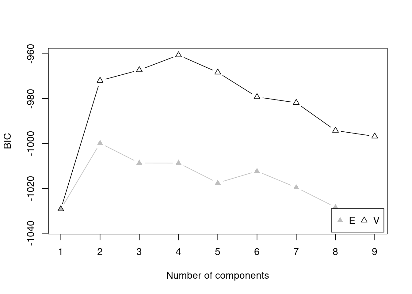
Code
Integrated Complete-data Likelihood (ICL) criterion:
          E          V
1 -1047.277 -1047.2769
2 -1025.144  -982.8331
3 -1099.777  -965.0763
4 -1091.611  -979.1174
5 -1116.242  -981.4868
6 -1112.402  -979.2345
7 -1114.819  -983.0710
8 -1131.472  -986.8153
9 -1145.924 -1002.0261

Top 3 models based on the ICL criterion:
      V,3       V,4       V,6
-965.0763 -979.1174 -979.2345 Best ICL values:
V,3 V,4 V,6
ICL -965.0763 -979.11739 -979.23450
ICL diff 0.0000 -14.04105 -14.15816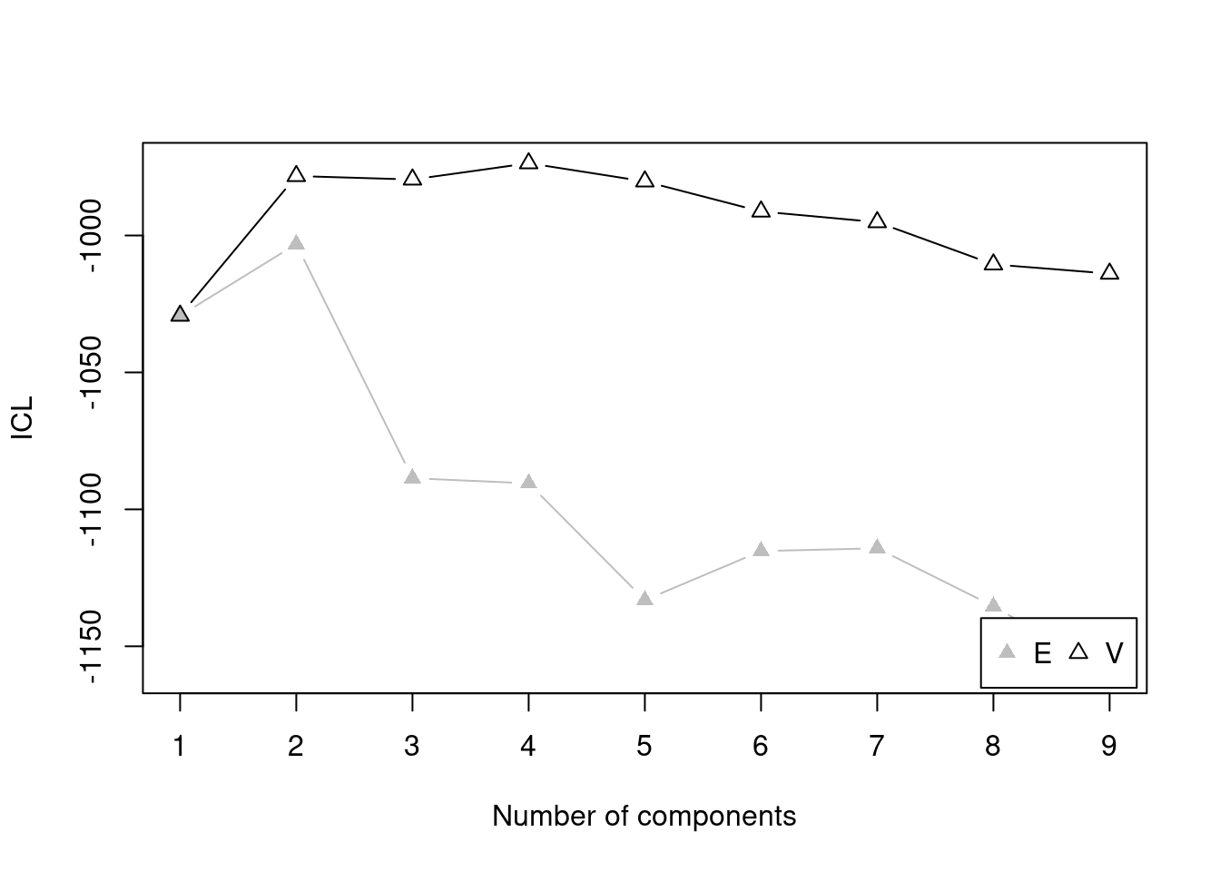
Code
tiersQB_bootstrap <- mclust::mclustBootstrapLRT(
  data = player_stats_seasonal_offense_recentQB$fantasyPoints,
  modelName = "V") # variable/unequal variance (for univariate data)

numTiersQB <- as.numeric(summary(tiersQB_bootstrap)[,"Length"][1]) # or could specify the number of teams manually

tiersQB_bootstrap
-------------------------------------------------------------
Bootstrap sequential LRT for the number of mixture components
-------------------------------------------------------------
Model = V
Replications = 999
LRTS bootstrap p-value
1 vs 2 83.257559 0.001
2 vs 3 36.294604 0.001
3 vs 4 4.663424 0.261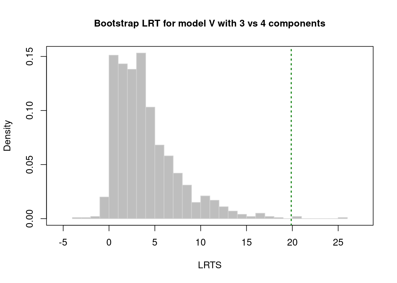
21.1.4.2.1.2 k-Means Clustering
Code
K-means clustering with 3 clusters of sizes 17, 20, 47

Cluster means:
       [,1]
1 147.08706
2 292.00200
3  21.16468

Clustering vector:
 [1] 2 3 3 3 3 2 2 3 3 3 1 2 1 2 1 3 3 3 3 2 2 3 3 2 3 3 3 1 1 2 3 2 3 3 2 3 2 1
[39] 3 1 1 3 2 2 3 3 1 2 3 3 1 3 3 2 1 3 3 1 3 2 3 1 3 3 2 3 3 3 3 2 3 1 1 3 3 3
[77] 2 3 1 3 1 3 3 3

Within cluster sum of squares by cluster:
[1] 18933.87 47116.32 26986.51
 (between_SS / total_SS =  91.9 %)

Available components:

[1] "cluster"      "centers"      "totss"        "withinss"     "tot.withinss"
[6] "betweenss"    "size"         "iter"         "ifault"
21.1.4.2.2 Running Backs
21.1.4.2.2.1 Model-Based Clustering
Code
Bayesian Information Criterion (BIC):
          E         V
1 -1861.107 -1861.107
2 -1811.582 -1725.933
3 -1821.675 -1711.104
4 -1805.732 -1713.045
5 -1815.817 -1694.542
6 -1825.901 -1706.984
7 -1794.275 -1722.425
8 -1804.364 -1730.058
9 -1806.258 -1736.878

Top 3 models based on the BIC criterion:
      V,5       V,6       V,3
-1694.542 -1706.984 -1711.104 Best BIC values:
V,5 V,6 V,3
BIC -1694.542 -1706.98389 -1711.10360
BIC diff 0.000 -12.44191 -16.56161
Code
Integrated Complete-data Likelihood (ICL) criterion:
          E         V
1 -1861.107 -1861.107
2 -1820.460 -1745.842
3 -1990.756 -1750.200
4 -1961.250 -1772.850
5 -2065.929 -1747.762
6 -2110.800 -1766.196
7 -2053.240 -1801.278
8 -2087.013 -1791.402
9 -2100.545 -1770.314

Top 3 models based on the ICL criterion:
      V,2       V,5       V,3
-1745.842 -1747.762 -1750.200 Best ICL values:
V,2 V,5 V,3
ICL -1745.842 -1747.762269 -1750.200480
ICL diff 0.000 -1.919844 -4.358056
Code
-------------------------------------------------------------
Bootstrap sequential LRT for the number of mixture components
-------------------------------------------------------------
Model        = V
Replications = 999
              LRTS bootstrap p-value
1 vs 2   150.30391             0.001
2 vs 3    29.95970             0.001
3 vs 4    13.18926             0.011
4 vs 5    33.63290             0.001
5 vs 6     2.68837             0.413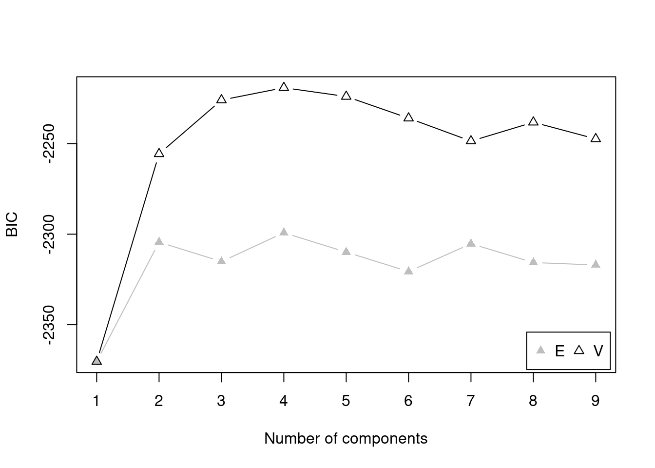
21.1.4.2.2.2 k-Means Clustering
Code
K-means clustering with 5 clusters of sizes 19, 6, 31, 32, 67

Cluster means:
        [,1]
1 230.303158
2 363.516667
3  47.883871
4 121.606875
5   8.841493

Clustering vector:
  [1] 5 4 5 5 4 5 3 5 1 3 5 5 4 4 2 4 5 5 3 1 3 5 5 4 5 5 4 1 5 3 4 2 4 5 5 5 1
 [38] 5 5 5 3 4 2 5 1 3 4 5 4 5 4 3 5 5 5 5 5 3 5 3 4 4 5 5 4 2 5 3 3 2 5 1 3 5
 [75] 1 3 3 3 2 4 5 1 5 5 3 5 5 4 3 5 3 5 1 1 5 4 3 4 1 3 5 3 4 3 5 5 5 5 4 5 3
[112] 4 5 5 5 4 1 4 3 5 3 3 5 1 1 5 5 5 4 1 4 5 5 3 5 1 1 5 5 1 5 3 5 5 4 4 4 3
[149] 5 4 5 3 4 1 5

Within cluster sum of squares by cluster:
[1] 17253.299  7905.428  6741.362 20410.611  3535.789
 (between_SS / total_SS =  96.0 %)

Available components:

[1] "cluster"      "centers"      "totss"        "withinss"     "tot.withinss"
[6] "betweenss"    "size"         "iter"         "ifault"
21.1.4.2.3 Wide Receivers
21.1.4.2.3.1 Model-Based Clustering
Code
Bayesian Information Criterion (BIC):
          E         V
1 -2802.433 -2802.433
2 -2728.279 -2658.661
3 -2739.278 -2618.080
4 -2709.854 -2611.538
5 -2720.837 -2624.395
6 -2731.809 -2631.475
7 -2700.395 -2646.194
8 -2711.738        NA
9 -2710.399        NA

Top 3 models based on the BIC criterion:
      V,4       V,3       V,5
-2611.538 -2618.080 -2624.395 Best BIC values:
V,4 V,3 V,5
BIC -2611.538 -2618.079552 -2624.39479
BIC diff 0.000 -6.541254 -12.85649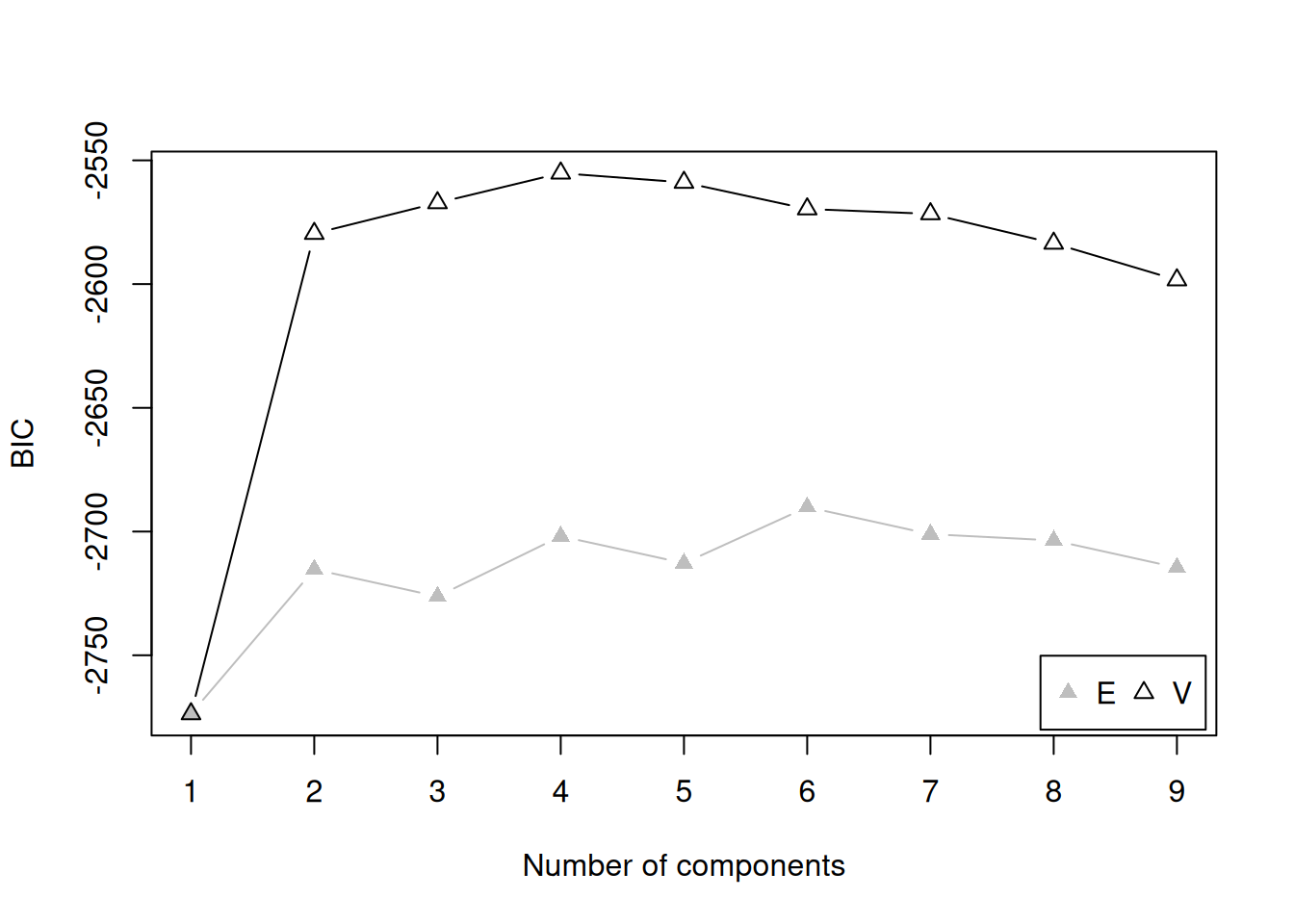
Code
Integrated Complete-data Likelihood (ICL) criterion:
          E         V
1 -2802.433 -2802.433
2 -2743.402 -2698.471
3 -2989.504 -2694.729
4 -2954.229 -2701.572
5 -3111.804 -2743.767
6 -3184.211 -2730.807
7 -3093.232 -2750.205
8 -3149.140        NA
9 -3118.240        NA

Top 3 models based on the ICL criterion:
      V,3       V,2       V,4
-2694.729 -2698.471 -2701.572 Best ICL values:
V,3 V,2 V,4
ICL -2694.729 -2698.470652 -2701.572327
ICL diff 0.000 -3.741961 -6.843636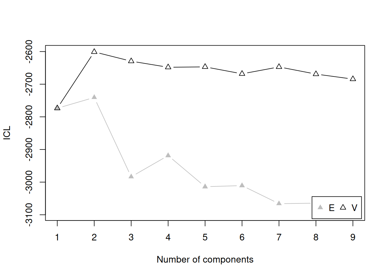
Code
tiersWR_bootstrap <- mclust::mclustBootstrapLRT(
  data = player_stats_seasonal_offense_recentWR$fantasyPoints,
  modelName = "V") # variable/unequal variance (for univariate data)

numTiersWR <- as.numeric(summary(tiersWR_bootstrap)[,"Length"][1]) # or could specify the number of teams manually

tiersWR_bootstrap
-------------------------------------------------------------
Bootstrap sequential LRT for the number of mixture components
-------------------------------------------------------------
Model = V
Replications = 999
LRTS bootstrap p-value
1 vs 2 160.239062 0.001
2 vs 3 57.048484 0.001
3 vs 4 23.008067 0.001
4 vs 5 3.610323 0.239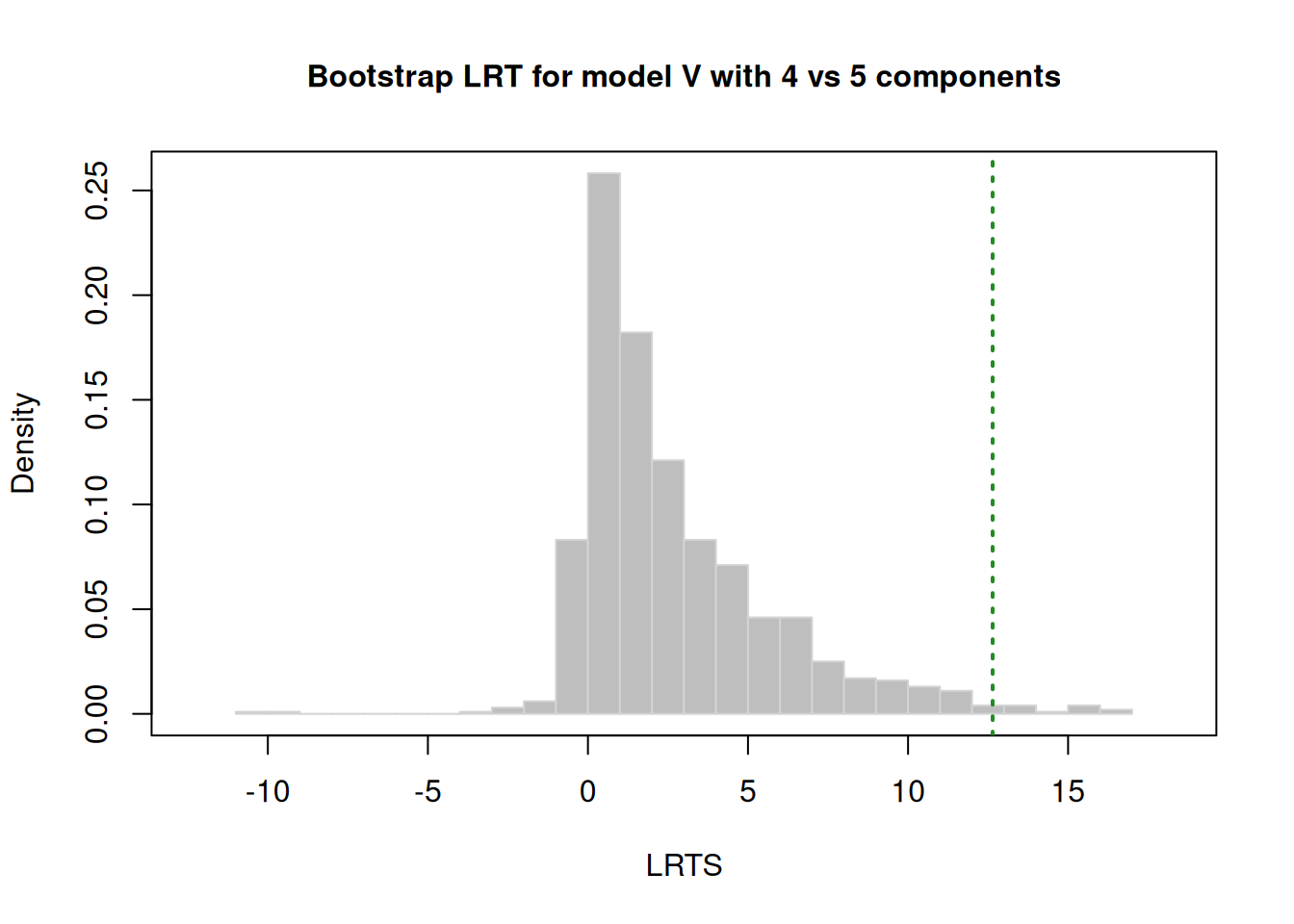
21.1.4.2.3.2 k-Means Clustering
Code
K-means clustering with 4 clusters of sizes 22, 120, 62, 38

Cluster means:
       [,1]
1 246.54545
2  14.65267
3  71.24194
4 153.41053

Clustering vector:
  [1] 1 2 3 4 2 2 1 2 3 2 2 2 2 2 2 2 3 2 4 2 2 2 3 3 2 3 2 1 2 4 2 3 2 1 3 4 2
 [38] 2 4 1 2 4 2 4 2 2 2 2 2 3 3 1 2 3 2 3 3 1 2 4 3 2 3 2 2 3 2 2 3 1 3 2 2 4
 [75] 2 4 2 2 3 1 3 2 2 3 3 2 3 1 3 2 3 2 2 4 2 2 3 2 2 3 2 3 2 2 2 2 1 2 2 4 1
[112] 4 3 4 3 3 4 2 2 3 2 4 2 2 4 3 2 3 1 2 4 3 2 3 2 4 2 2 4 3 3 2 2 4 2 3 2 4
[149] 2 2 3 4 4 2 2 3 2 4 2 4 4 3 2 2 3 2 2 1 1 3 2 2 2 1 2 2 3 4 2 3 1 4 2 4 4
[186] 3 2 3 2 2 2 4 4 2 4 2 2 2 2 2 2 2 1 3 2 2 2 2 1 4 1 3 2 2 3 2 3 3 4 2 2 4
[223] 2 2 2 3 3 3 3 3 2 1 2 3 3 2 3 2 4 3 1 2

Within cluster sum of squares by cluster:
[1] 62935.41 17676.37 20778.91 30266.65
 (between_SS / total_SS =  90.9 %)

Available components:

[1] "cluster"      "centers"      "totss"        "withinss"     "tot.withinss"
[6] "betweenss"    "size"         "iter"         "ifault"
21.1.4.2.4 Tight Ends
21.1.4.2.4.1 Model-Based Clustering
Code
Bayesian Information Criterion (BIC):
          E         V
1 -1510.118 -1510.118
2 -1475.580 -1423.521
3 -1485.410 -1386.193
4 -1495.249 -1391.099
5 -1483.308 -1403.054
6 -1493.143 -1415.314
7 -1500.533 -1424.818
8 -1510.340 -1435.253
9 -1520.205 -1448.297

Top 3 models based on the BIC criterion:
      V,3       V,4       V,5
-1386.193 -1391.099 -1403.054 Best BIC values:
V,3 V,4 V,5
BIC -1386.193 -1391.098962 -1403.05419
BIC diff 0.000 -4.906124 -16.86135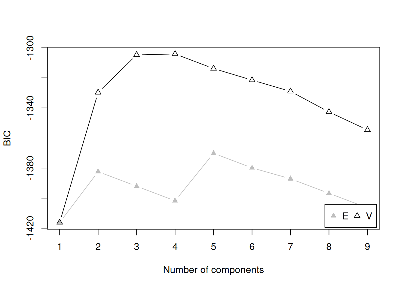
Code
Integrated Complete-data Likelihood (ICL) criterion:
          E         V
1 -1510.118 -1510.118
2 -1485.909 -1446.680
3 -1628.797 -1417.288
4 -1683.964 -1442.330
5 -1695.404 -1466.808
6 -1734.052 -1497.596
7 -1747.610 -1484.558
8 -1766.876 -1499.674
9 -1819.549 -1513.339

Top 3 models based on the ICL criterion:
      V,3       V,4       V,2
-1417.288 -1442.330 -1446.680 Best ICL values:
V,3 V,4 V,2
ICL -1417.288 -1442.32971 -1446.68023
ICL diff 0.000 -25.04136 -29.39187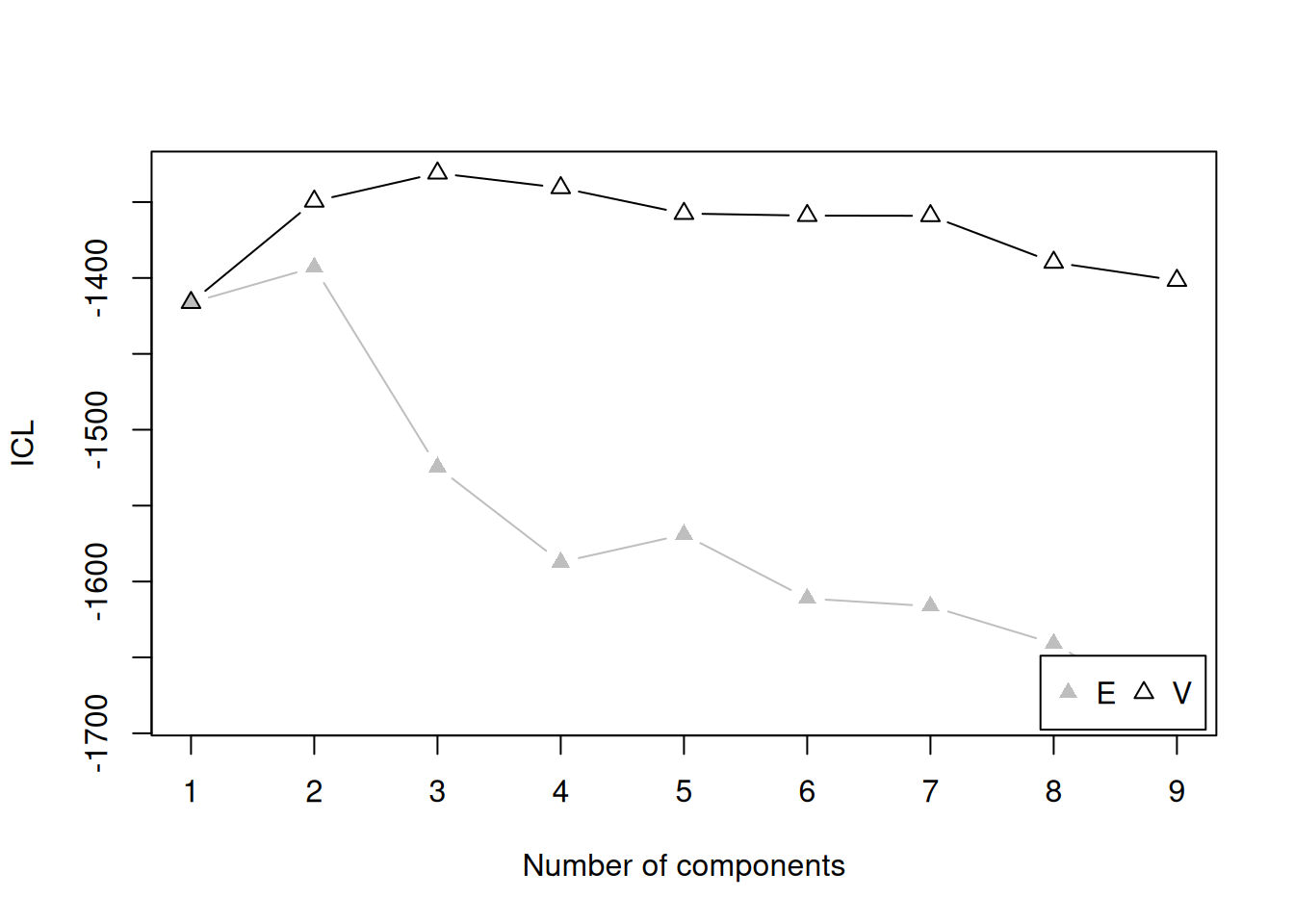
Code
tiersTE_bootstrap <- mclust::mclustBootstrapLRT(
  data = player_stats_seasonal_offense_recentTE$fantasyPoints,
  modelName = "V") # variable/unequal variance (for univariate data)

numTiersTE <- as.numeric(summary(tiersTE_bootstrap)[,"Length"][1]) # or could specify the number of teams manually

tiersTE_bootstrap
-------------------------------------------------------------
Bootstrap sequential LRT for the number of mixture components
-------------------------------------------------------------
Model = V
Replications = 999
LRTS bootstrap p-value
1 vs 2 101.335350 0.001
2 vs 3 52.065920 0.001
3 vs 4 9.831840 0.041
4 vs 5 2.782735 0.407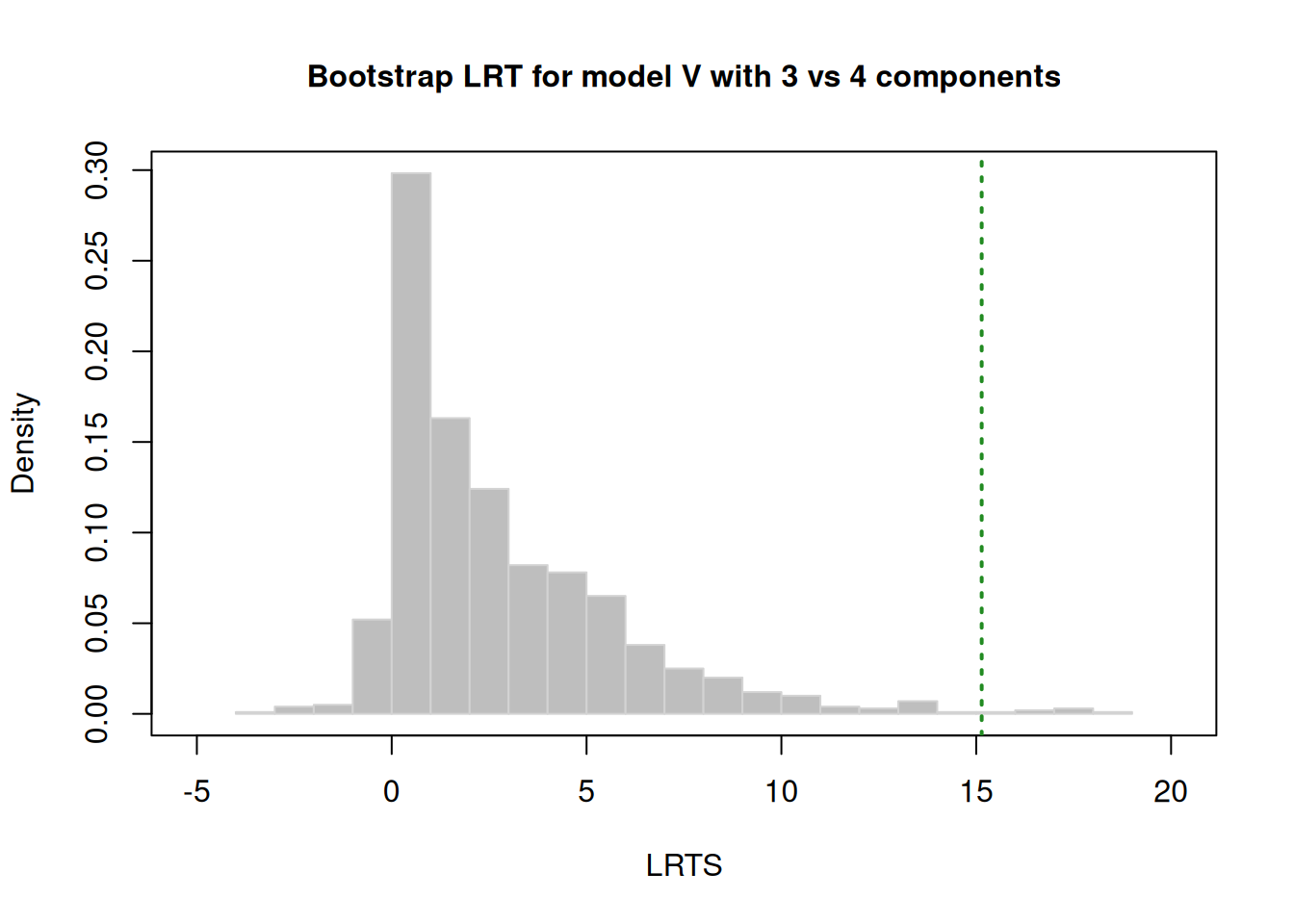
21.1.4.2.4.2 k-Means Clustering
Code
K-means clustering with 4 clusters of sizes 69, 12, 33, 22

Cluster means:
       [,1]
1  10.18551
2 196.06667
3  53.64545
4 114.05000

Clustering vector:
  [1] 4 3 1 1 1 1 3 1 1 1 1 1 1 4 3 2 3 4 1 1 1 1 3 1 4 1 4 3 1 2 3 2 4 2 3 3 4
 [38] 1 4 3 4 1 1 3 1 1 3 3 1 4 1 2 1 1 3 4 2 1 1 2 3 1 3 3 1 1 3 2 4 1 1 1 3 1
 [75] 1 1 4 3 1 1 3 1 1 1 2 1 1 3 3 1 1 4 4 3 3 3 3 1 1 1 1 3 3 4 4 1 1 1 1 1 1
[112] 1 4 1 1 4 1 3 1 3 4 1 1 3 2 1 2 1 4 1 3 2 1 1 4 1

Within cluster sum of squares by cluster:
[1]  5569.546 17719.347  7777.442  6996.475
 (between_SS / total_SS =  92.3 %)

Available components:

[1] "cluster"      "centers"      "totss"        "withinss"     "tot.withinss"
[6] "betweenss"    "size"         "iter"         "ifault"
21.1.4.3 Fit the Cluster Model to the Optimal Number of Tiers
21.1.4.3.1 Quarterbacks
In our data, all of the following models are equivalent—i.e., they result in the same unequal variance model with a 4-cluster solution—but they arrive there in different ways. We can fit the cluster model to the optimal number of tiers using the mclust::Mclust() function.
Code
mclust::Mclust(
  data = player_stats_seasonal_offense_recentQB$fantasyPoints,
  G = numTiersQB,
)

mclust::Mclust(
  data = player_stats_seasonal_offense_recentQB$fantasyPoints,
  G = 4,
)

mclust::Mclust(
  data = player_stats_seasonal_offense_recentQB$fantasyPoints,
)

mclust::Mclust(
  data = player_stats_seasonal_offense_recentQB$fantasyPoints,
  x = tiersQB_bic
)
Let’s fit one of these:
Here are the number of players that are in each of the four clusters (i.e., tiers):
21.1.4.3.2 Running Backs
Here are the number of players that are in each of the four clusters (i.e., tiers):
21.1.4.3.3 Wide Receivers
Here are the number of players that are in each of the four clusters (i.e., tiers):
21.1.4.3.4 Tight Ends
Here are the number of players that are in each of the four clusters (i.e., tiers):
21.1.4.4 Plot the Tiers
We can merge the player’s classification into the dataset and plot each player’s classification.
21.1.4.4.1 Quarterbacks
Code
player_stats_seasonal_offense_recentQB$tier <- clusterModelQBs$classification

player_stats_seasonal_offense_recentQB <- player_stats_seasonal_offense_recentQB %>%
  mutate(
    tier = factor(max(tier, na.rm = TRUE) + 1 - tier)
  )

player_stats_seasonal_offense_recentQB$position_rank <- rank(
  player_stats_seasonal_offense_recentQB$fantasyPoints * -1,
  na.last = "keep",
  ties.method = "min")

plot_qbTiers <- ggplot2::ggplot(
  data = player_stats_seasonal_offense_recentQB,
  mapping = aes(
    x = fantasyPoints,
    y = position_rank,
    color = tier
  )) +
  geom_point(
    aes(
      text = player_display_name # add player name for mouse over tooltip
  )) +
  scale_y_continuous(trans = "reverse") +
  coord_cartesian(clip = "off") +
  labs(
    x = "Projected Points",
    y = "Position Rank",
    title = "Quarterback Fantasy Points by Tier",
    color = "Tier") +
  theme_classic() +
  theme(legend.position = "top")

plotly::ggplotly(plot_qbTiers)21.1.4.4.2 Running Backs
Code
player_stats_seasonal_offense_recentRB$tier <- clusterModelRBs$classification

player_stats_seasonal_offense_recentRB <- player_stats_seasonal_offense_recentRB %>%
  mutate(
    tier = factor(max(tier, na.rm = TRUE) + 1 - tier)
  )

player_stats_seasonal_offense_recentRB$position_rank <- rank(
  player_stats_seasonal_offense_recentRB$fantasyPoints * -1,
  na.last = "keep",
  ties.method = "min")

plot_rbTiers <- ggplot2::ggplot(
  data = player_stats_seasonal_offense_recentRB,
  mapping = aes(
    x = fantasyPoints,
    y = position_rank,
    color = tier
  )) +
  geom_point(
    aes(
      text = player_display_name # add player name for mouse over tooltip
  )) +
  scale_y_continuous(trans = "reverse") +
  coord_cartesian(clip = "off") +
  labs(
    x = "Projected Points",
    y = "Position Rank",
    title = "Running Back Fantasy Points by Tier",
    color = "Tier") +
  theme_classic() +
  theme(legend.position = "top")

plotly::ggplotly(plot_rbTiers)21.1.4.4.3 Wide Receivers
Code
player_stats_seasonal_offense_recentWR$tier <- clusterModelWRs$classification

player_stats_seasonal_offense_recentWR <- player_stats_seasonal_offense_recentWR %>%
  mutate(
    tier = factor(max(tier, na.rm = TRUE) + 1 - tier)
  )

player_stats_seasonal_offense_recentWR$position_rank <- rank(
  player_stats_seasonal_offense_recentWR$fantasyPoints * -1,
  na.last = "keep",
  ties.method = "min")

plot_wrTiers <- ggplot2::ggplot(
  data = player_stats_seasonal_offense_recentWR,
  mapping = aes(
    x = fantasyPoints,
    y = position_rank,
    color = tier
  )) +
  geom_point(
    aes(
      text = player_display_name # add player name for mouse over tooltip
  )) +
  scale_y_continuous(trans = "reverse") +
  coord_cartesian(clip = "off") +
  labs(
    x = "Projected Points",
    y = "Position Rank",
    title = "Wide Receiver Fantasy Points by Tier",
    color = "Tier") +
  theme_classic() +
  theme(legend.position = "top")

plotly::ggplotly(plot_wrTiers)21.1.4.4.4 Tight Ends
Code
player_stats_seasonal_offense_recentTE$tier <- clusterModelTEs$classification

player_stats_seasonal_offense_recentTE <- player_stats_seasonal_offense_recentTE %>%
  mutate(
    tier = factor(max(tier, na.rm = TRUE) + 1 - tier)
  )

player_stats_seasonal_offense_recentTE$position_rank <- rank(
  player_stats_seasonal_offense_recentTE$fantasyPoints * -1,
  na.last = "keep",
  ties.method = "min")

plot_teTiers <- ggplot2::ggplot(
  data = player_stats_seasonal_offense_recentTE,
  mapping = aes(
    x = fantasyPoints,
    y = position_rank,
    color = tier
  )) +
  geom_point(
    aes(
      text = player_display_name # add player name for mouse over tooltip
  )) +
  scale_y_continuous(trans = "reverse") +
  coord_cartesian(clip = "off") +
  labs(
    x = "Projected Points",
    y = "Position Rank",
    title = "Tight End Fantasy Points by Tier",
    color = "Tier") +
  theme_classic() +
  theme(legend.position = "top")

plotly::ggplotly(plot_teTiers)21.1.5 Types of Wide Receivers
Code
# Compute Advanced PFR Stats by Career
pfrVars <- nfl_advancedStatsPFR_seasonal %>%
  select(pocket_time.pass:cmp_percent.def, g, gs) %>%
  names()

weightedAverageVars <- c(
  "pocket_time.pass",
  "ybc_att.rush","yac_att.rush",
  "ybc_r.rec","yac_r.rec","adot.rec","rat.rec",
  "yds_cmp.def","yds_tgt.def","dadot.def","m_tkl_percent.def","rat.def"
)

recomputeVars <- c(
  "drop_pct.pass", # drops.pass / pass_attempts.pass
  "bad_throw_pct.pass", # bad_throws.pass / pass_attempts.pass
  "on_tgt_pct.pass", # on_tgt_throws.pass / pass_attempts.pass
  "pressure_pct.pass", # times_pressured.pass / pass_attempts.pass
  "drop_percent.rec", # drop.rec / tgt.rec
  "rec_br.rec", # rec.rec / brk_tkl.rec
  "cmp_percent.def" # cmp.def / tgt.def
)

sumVars <- pfrVars[pfrVars %ni% c(
  weightedAverageVars, recomputeVars,
  "merge_name", "loaded.pass", "loaded.rush", "loaded.rec", "loaded.def")]

nfl_advancedStatsPFR_career <- nfl_advancedStatsPFR_seasonal %>%
  group_by(pfr_id, merge_name) %>%
  summarise(
    across(all_of(weightedAverageVars), ~ weighted.mean(.x, w = g, na.rm = TRUE)),
    across(all_of(sumVars), ~ sum(.x, na.rm = TRUE)),
    .groups = "drop") %>%
  mutate(
    drop_pct.pass = drops.pass / pass_attempts.pass,
    bad_throw_pct.pass = bad_throws.pass / pass_attempts.pass,
    on_tgt_pct.pass = on_tgt_throws.pass / pass_attempts.pass,
    pressure_pct.pass = times_pressured.pass / pass_attempts.pass,
    drop_percent.rec = drop.rec / tgt.rec,
    rec_br.rec = drop.rec / tgt.rec,
    cmp_percent.def = cmp.def / tgt.def
  )

uniqueCases <- nfl_advancedStatsPFR_seasonal %>% select(pfr_id, merge_name, gsis_id) %>% unique()

uniqueCases %>%
  group_by(pfr_id) %>%
  filter(n() > 1)
Code
nfl_advancedStatsPFR_seasonal <- nfl_advancedStatsPFR_seasonal %>%
  filter(pfr_id != "WillMa06" | merge_name != "MARCUSWILLIAMS" | !is.na(gsis_id))


nfl_advancedStatsPFR_career <- left_join(
  nfl_advancedStatsPFR_career,
  nfl_advancedStatsPFR_seasonal %>% select(pfr_id, merge_name, gsis_id) %>% unique(),
  by = c("pfr_id", "merge_name")
)

# Compute Player Stats Per Season
player_stats_seasonal_careerWRs <- player_stats_seasonal %>%
  filter(position == "WR") %>%
  group_by(player_id) %>%
  summarise(
    across(all_of(c("targets", "receptions", "receiving_air_yards")), ~ weighted.mean(.x, w = games, na.rm = TRUE)),
    .groups = "drop")

# Drop players with no receiving air yards
player_stats_seasonal_careerWRs <- player_stats_seasonal_careerWRs %>%
  filter(receiving_air_yards != 0) %>%
  rename(
    targets_per_season = targets,
    receptions_per_season = receptions,
    receiving_air_yards_per_season = receiving_air_yards
  )

# Merge
playerListToMerge <- list(
  nfl_players %>% select(gsis_id, display_name, position, height, weight),
  nfl_combine %>% select(gsis_id, vertical, forty, ht, wt),
  player_stats_seasonal_careerWRs %>% select(player_id, targets_per_season, receptions_per_season, receiving_air_yards_per_season) %>%
    rename(gsis_id = player_id),
  nfl_actualStats_career_player_inclPost %>% select(player_id, receptions, targets, receiving_air_yards, air_yards_share, target_share) %>%
    rename(gsis_id = player_id),
  nfl_advancedStatsPFR_career %>% select(gsis_id, adot.rec, rec.rec, brk_tkl.rec, drop.rec, drop_percent.rec)
)

merged_data <- playerListToMerge %>%
  reduce(
    full_join,
    by = c("gsis_id"),
    na_matches = "never")
Additional processing:
Code
merged_data <- merged_data %>%
  mutate(
    height_coalesced = coalesce(height, ht),
    weight_coalesced = coalesce(weight, wt),
    receptions_coalesced = pmax(receptions, rec.rec, na.rm = TRUE),
    receiving_air_yards_per_rec = receiving_air_yards / receptions
  )

merged_data$receiving_air_yards_per_rec[which(merged_data$receptions == 0)] <- 0

merged_dataWRs <- merged_data %>%
  filter(position == "WR")

merged_dataWRs_cluster <- merged_dataWRs %>%
  filter(receptions_coalesced >= 100) %>% # keep WRs with at least 100 receptions
  select(gsis_id, display_name, vertical, forty, height_coalesced, weight_coalesced, adot.rec, drop_percent.rec, receiving_air_yards_per_rec, brk_tkl.rec, receptions_per_season) %>% #targets_per_season, receiving_air_yards_per_season, air_yards_share, target_share
  na.omit()
21.1.5.1 Identify the Number of WR Types
21.1.5.1.1 Model-Based Clustering
Code
Bayesian Information Criterion (BIC):
        EII       VII       EEI       VEI       EVI       VVI       EEE
1 -9339.068 -9339.068 -5690.468 -5690.468 -5690.468 -5690.468 -5431.024
2 -8883.259 -8858.480 -5622.236 -5609.646 -5495.927 -5614.682 -5460.607
3 -8737.861 -8662.946 -5542.102 -5547.634 -5465.130 -5463.333 -5443.739
4 -8645.143 -8603.562 -5539.221 -5497.289 -5448.970 -5445.734 -5421.107
5 -8514.498 -8453.417 -5535.805 -5515.045 -5455.561 -5475.259 -5398.793
6 -8494.136 -8481.139 -5544.796 -5495.332 -5488.317 -5484.415 -5424.334
7 -8510.170 -8408.225 -5504.486 -5502.386 -5498.312 -5482.056 -5461.462
8 -8423.951 -8409.397 -5579.370 -5518.477 -5530.542 -5531.024 -5511.150
9 -8433.392        NA -5530.196        NA        NA        NA -5442.727
        VEE       EVE       VVE       EEV       VEV       EVV       VVV
1 -5431.024 -5431.024 -5431.024 -5431.024 -5431.024 -5431.024 -5431.024
2 -5336.709 -5191.280 -5214.259 -5308.606 -5312.351 -5333.094 -5339.801
3 -5324.507 -5130.666 -5126.969 -5401.274 -5346.723 -5362.450 -5347.270
4 -5345.735 -5177.203 -5185.212 -5507.634 -5482.750 -5559.983 -5567.016
5        NA        NA        NA -5586.417 -5585.968        NA        NA
6        NA        NA        NA -5817.980 -5808.809        NA        NA
7        NA        NA        NA -5882.022 -5929.968        NA        NA
8        NA        NA        NA -6032.990 -6073.931        NA        NA
9        NA        NA        NA -6240.289        NA        NA        NA

Top 3 models based on the BIC criterion:
    VVE,3     EVE,3     EVE,4
-5126.969 -5130.666 -5177.203 Best BIC values:
VVE,3 EVE,3 EVE,4
BIC -5126.969 -5130.665897 -5177.20254
BIC diff 0.000 -3.697043 -50.23369
Code
Integrated Complete-data Likelihood (ICL) criterion:
        EII       VII       EEI       VEI       EVI       VVI       EEE
1 -9339.068 -9339.068 -5690.468 -5690.468 -5690.468 -5690.468 -5431.024
2 -8889.848 -8867.147 -5638.757 -5622.174 -5513.720 -5634.275 -5475.575
3 -8751.310 -8674.859 -5558.314 -5562.591 -5493.065 -5488.152 -5464.792
4 -8661.489 -8617.935 -5563.778 -5512.508 -5469.768 -5469.537 -5443.638
5 -8528.010 -8467.045 -5555.370 -5535.128 -5483.694 -5492.409 -5419.665
6 -8508.045 -8498.110 -5569.096 -5519.950 -5508.170 -5500.430 -5452.643
7 -8529.643 -8421.999 -5531.100 -5519.200 -5513.558 -5496.680 -5488.749
8 -8439.277 -8423.579 -5608.220 -5537.328 -5546.773 -5548.607 -5534.899
9 -8446.448        NA -5556.562        NA        NA        NA -5463.056
        VEE       EVE       VVE       EEV       VEV       EVV       VVV
1 -5431.024 -5431.024 -5431.024 -5431.024 -5431.024 -5431.024 -5431.024
2 -5338.177 -5202.559 -5221.623 -5309.413 -5314.330 -5335.774 -5344.901
3 -5328.248 -5154.713 -5144.214 -5405.795 -5348.675 -5369.905 -5355.914
4 -5363.827 -5205.693 -5210.566 -5517.421 -5494.439 -5572.190 -5573.007
5        NA        NA        NA -5595.267 -5595.666        NA        NA
6        NA        NA        NA -5824.201 -5816.763        NA        NA
7        NA        NA        NA -5883.567 -5931.816        NA        NA
8        NA        NA        NA -6034.555 -6074.519        NA        NA
9        NA        NA        NA -6242.758        NA        NA        NA

Top 3 models based on the ICL criterion:
    VVE,3     EVE,3     EVE,2
-5144.214 -5154.713 -5202.559 Best ICL values:
VVE,3 EVE,3 EVE,2
ICL -5144.214 -5154.71272 -5202.5593
ICL diff 0.000 -10.49899 -58.3456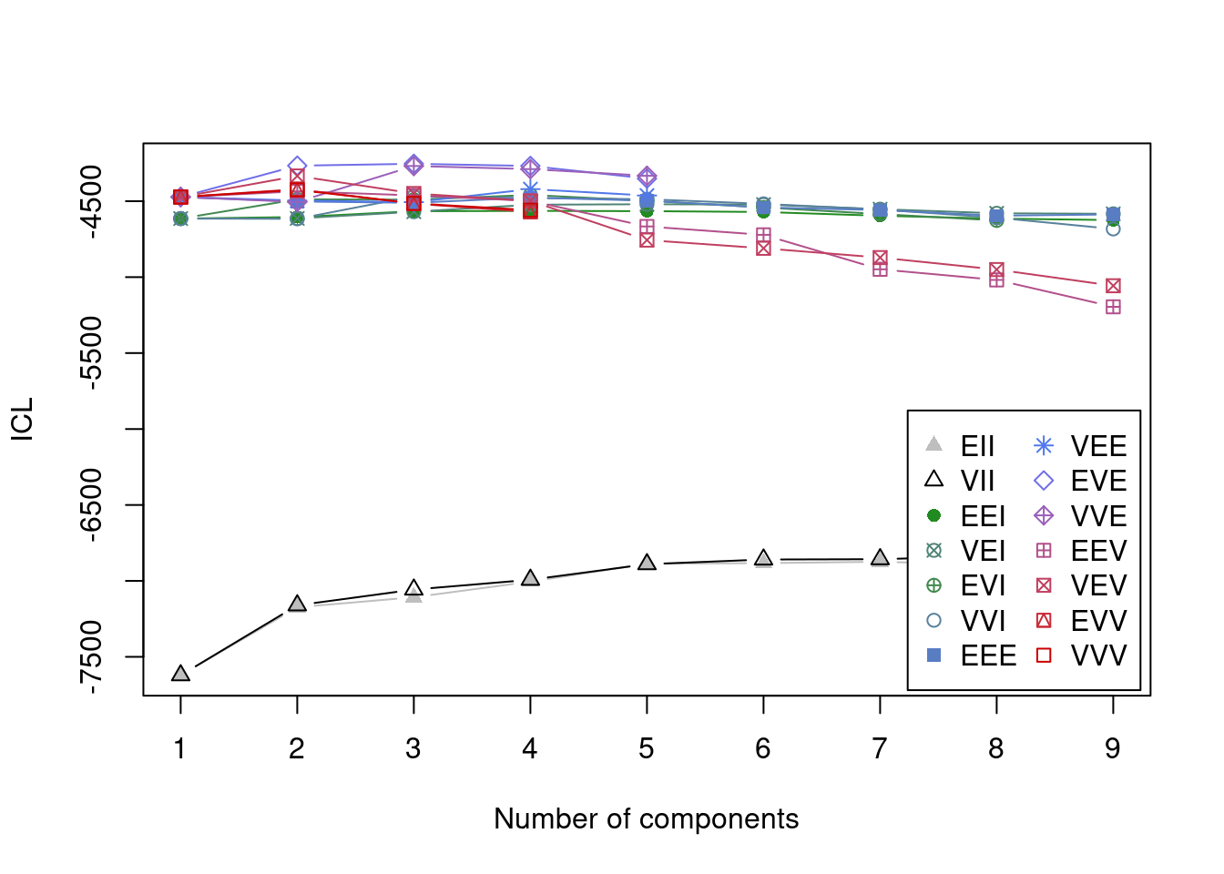
Based on the cluster analyses, it appears that three clusters are the best fit to the data.
We can also use the tidyLPA package (Rosenberg et al., 2018; Rosenberg & van Lissa, 2021), which provides an interface to the mclust package (Fraley et al., 2024; Scrucca et al., 2023).
Code
# model 1 (EEI): Equal variances and covariances fixed to 0
# model 2 (VVI): Varying variances and covariances fixed to 0
# model 3 (EEE): Equal variances and equal covariances
# model 4      : Varying variances and equal covariances (not able to be fit w/ mclust but can be fit using package = "mplus", if installed)
# model 5      : Equal variances and varying covariances (not able to be fit w/ mclust but can be fit using package = "mplus", if installed)
# model 6 (VVV): Varying variances and varying covariances

wrTypes_lpa_classes <- tidyLPA::estimate_profiles(
  df = merged_dataWRs_cluster %>% select(-gsis_id, -display_name),
  n_profiles = 1:6,
  models = c(1, 2, 3) #c(1, 2, 3, 6) takes too long to run because of the model with varying variances and varying covariances (model 6)
)

wrTypes_lpa_classes
tidyLPA analysis using mclust:
Model Classes AIC BIC Entropy prob_min prob_max n_min n_max BLRT_p
1 1 1 5637.65 5690.47 1.00 1.00 1.00 1.00 1.00
2 1 2 5540.07 5622.24 0.81 0.92 0.97 0.39 0.61 0.01
3 1 3 5430.59 5542.10 0.88 0.94 0.96 0.15 0.45 0.01
4 1 4 5398.37 5539.22 0.85 0.86 0.95 0.13 0.37 0.01
5 1 5 5365.61 5535.81 0.89 0.91 0.98 0.02 0.40 0.01
6 1 6 5345.25 5544.80 0.90 0.83 1.00 0.04 0.39 0.01
7 2 1 5637.65 5690.47 1.00 1.00 1.00 1.00 1.00
8 2 2 5506.11 5614.68 0.79 0.91 0.96 0.39 0.61 0.01
9 2 3 5299.00 5463.33 0.84 0.90 0.94 0.27 0.42 0.01
10 2 4 5225.65 5445.73 0.87 0.88 0.97 0.18 0.31 0.01
11 2 5 5199.42 5475.26 0.90 0.91 0.98 0.06 0.34 0.01
12 2 6 5152.82 5484.42 0.92 0.94 0.98 0.06 0.29 0.01
13 3 1 5344.56 5608.67 1.00 1.00 1.00 1.00 1.00
14 3 2 5344.80 5638.25 0.80 0.95 0.95 0.45 0.55 0.35
15 3 3 5298.59 5621.38 0.85 0.91 0.97 0.10 0.49 0.01
16 3 4 5246.61 5598.75 0.88 0.91 1.00 0.04 0.47 0.01
17 3 5 5194.95 5576.43 0.90 0.92 1.00 0.04 0.47 0.01
18 3 6 5191.15 5601.97 0.88 0.86 1.00 0.04 0.37 0.18Code
Compare tidyLPA solutions:

 Model Classes AIC      BIC      Entropy BLRT_p
 1     1       5637.648 5690.468 1.000
 1     2       5540.071 5622.236 0.811   0.010
 1     3       5430.592 5542.102 0.877   0.010
 1     4       5398.366 5539.221 0.854   0.010
 1     5       5365.606 5535.805 0.894   0.010
 1     6       5345.252 5544.796 0.897   0.010
 2     1       5637.648 5690.468 1.000
 2     2       5506.107 5614.682 0.795   0.010
 2     3       5299.002 5463.333 0.835   0.010
 2     4       5225.648 5445.734 0.866   0.010
 2     5       5199.419 5475.259 0.903   0.010
 2     6       5152.820 5484.415 0.922   0.010
 3     1       5344.562 5608.665 1.000
 3     2       5344.800 5638.248 0.801   0.347
 3     3       5298.588 5621.380 0.852   0.010
 3     4       5246.612 5598.749 0.877   0.010
 3     5       5194.953 5576.434 0.905   0.010
 3     6       5191.148 5601.975 0.878   0.178

Best model according to AIC is Model 2 with 6 classes.
Best model according to BIC is Model 2 with 4 classes.
Best model according to Entropy is Model NA with NA classes.
Best model according to BLRT_p is Model NA with NA classes.

An analytic hierarchy process, based on the fit indices AIC, AWE, BIC, CLC, and KIC (Akogul & Erisoglu, 2017), suggests the best solution is Model 2 with 6 classes.
Code
tidyLPA analysis using mclust:

  Model Classes     AIC     BIC Entropy prob_min prob_max n_min n_max BLRT_p
1 3 3 5298.59 5621.38 0.85 0.91 0.97 0.10 0.49 0.0121.1.5.1.2 k-Means Clustering
Code
K-means clustering with 3 clusters of sizes 47, 51, 41

Cluster means:
  vertical    forty height_coalesced weight_coalesced adot.rec drop_percent.rec
1 36.00000 4.428936         70.82979         186.4468 10.68079       0.05185007
2 36.40196 4.491176         73.92157         209.9608 11.24639       0.05172073
3 36.20732 4.476829         73.07317         205.4878 10.17858       0.04402159
  receiving_air_yards_per_rec brk_tkl.rec receptions_per_season
1                    16.74456    8.574468              44.74959
2                    20.79870    4.666667              35.79269
3                    15.96100   25.780488              76.58586

Clustering vector:
  [1] 3 3 1 2 1 2 3 3 3 2 2 3 1 3 2 3 2 3 2 1 2 3 2 2 3 2 3 1 2 3 3 1 2 3 3 1 1
 [38] 1 2 3 3 2 3 2 2 2 3 2 2 2 1 1 2 3 3 3 1 1 3 1 3 2 1 1 3 2 1 1 2 1 1 1 2 1
 [75] 1 3 3 3 2 2 2 2 2 1 3 2 1 2 2 1 1 1 2 1 3 3 2 3 1 2 3 3 2 1 2 2 1 1 2 3 1
[112] 1 1 2 1 2 1 2 2 3 1 2 1 2 3 2 1 1 1 2 3 1 3 1 1 1 2 3 2

Within cluster sum of squares by cluster:
[1] 15612.02 15656.87 24373.77
 (between_SS / total_SS =  54.7 %)

Available components:

[1] "cluster"      "centers"      "totss"        "withinss"     "tot.withinss"
[6] "betweenss"    "size"         "iter"         "ifault"
21.1.5.2 Fit the Cluster Model to the Optimal Number of WR Types
Code
----------------------------------------------------
Gaussian finite mixture model fitted by EM algorithm
----------------------------------------------------

Mclust VVE (ellipsoidal, equal orientation) model with 3 components:

 log-likelihood   n df       BIC       ICL
      -2336.499 139 92 -5126.969 -5144.214

Clustering table:
 1  2  3
34 21 84
21.1.5.3 Plots of the Cluster Model
21.1.5.4 Interpreting the Clusters
 1  2  3
34 21 84
Code
[,1] [,2] [,3]
type 1.00 2.00 3.00
vertical 36.01 36.21 36.29
forty 4.47 4.46 4.47
height_coalesced 72.91 72.90 72.44
weight_coalesced 204.32 205.76 197.95
adot.rec 10.08 11.96 10.70
drop_percent.rec 0.04 0.06 0.05
receiving_air_yards_per_rec 15.72 21.95 17.94
brk_tkl.rec 29.35 0.71 8.15
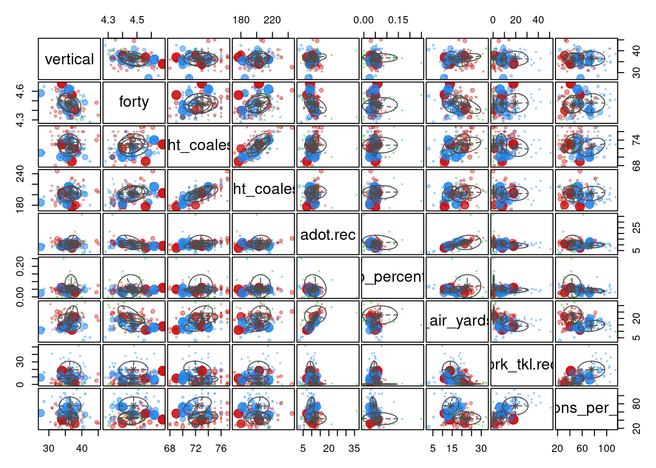
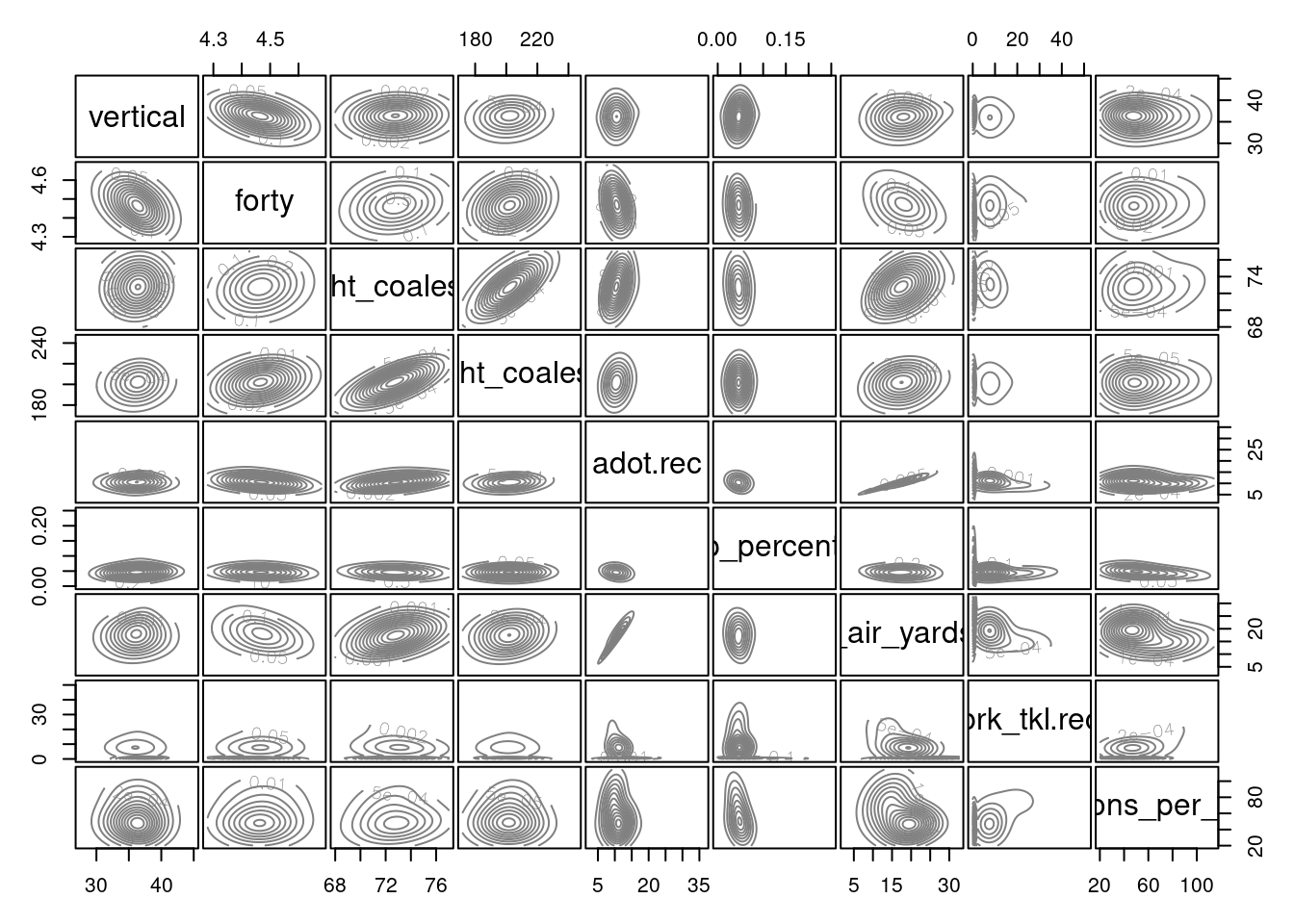
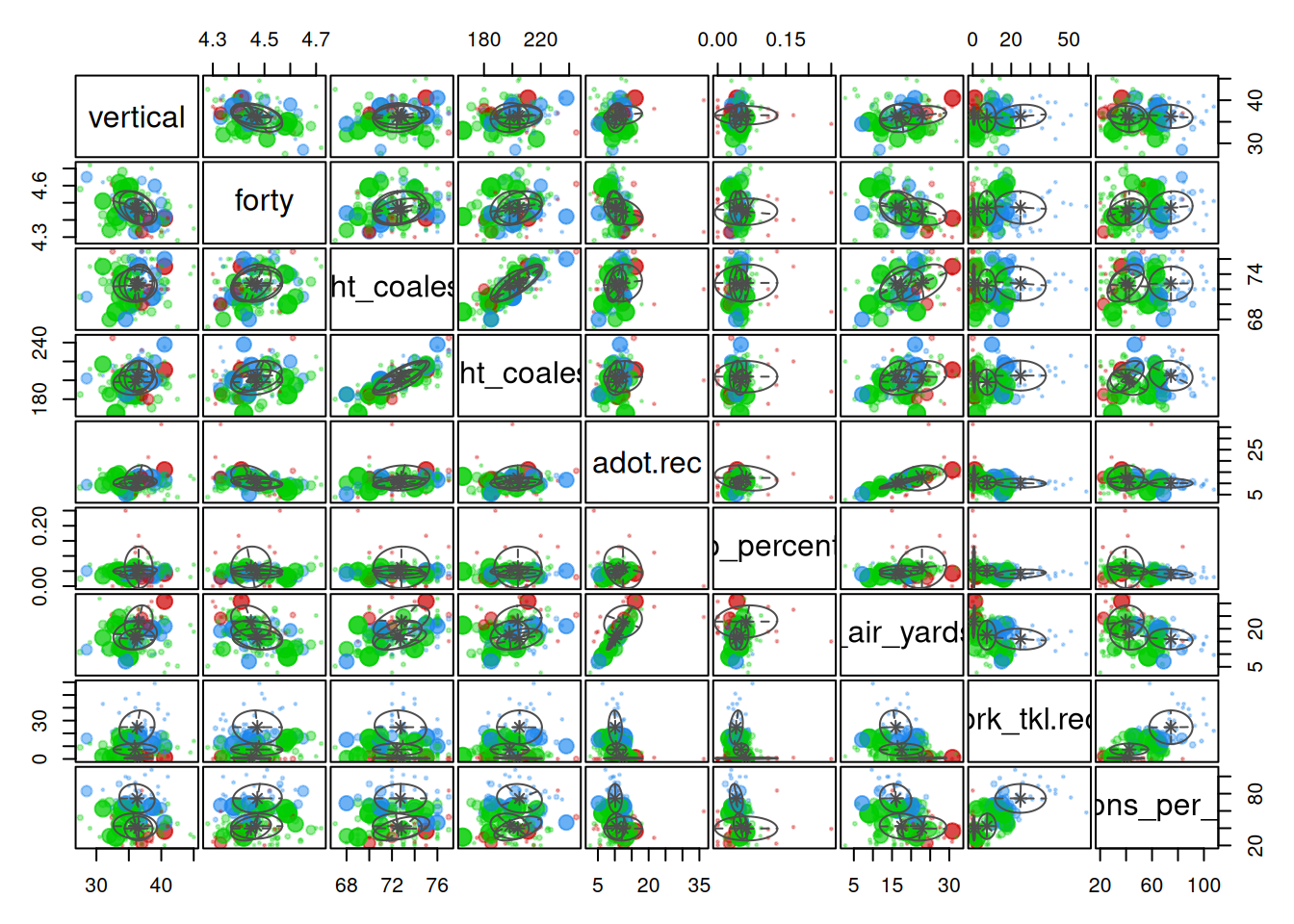
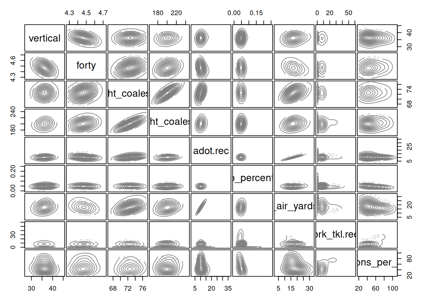
receptions_per_season 77.33 37.72 43.42Based on this analysis (and the variables included), there appear to be three types of Wide Receivers. We examined the following variables: the player’s vertical jump in the NFL Combine,40-yard-dash time in the NFL Combine, height, weight, average depth of target, drop percentage, receiving air yards per reception, broken tackles, and receptions per season.
Type 1 Wide Receivers included the Elite WR1s who are strong possession receivers (note: not all players in a given cluster map on perfectly to the typology—i.e., not all Type 1 Wide Receivers are elite WR1s). They tended to have the lowest drop percentage, the shortest average depth of target, and the fewest receiving air yards per reception. They tended to have the most receptions per season and break the most tackles.
Type 2 Wide Receivers included the consistent contributor, WR2 types. They had fewer receptions and fewer broken tackles than Type 1 Wide Receivers. Their average depth of target was longer than Type 1, and they had more receiving air yards per reception than Type 1.
Type 3 Wide Receivers included the deep threats. They had the greatest average depth of target and the most receiving yards per reception. However, they also had the fewest receptions, the highest drop percentage, and the fewest broken tackles. Thus, they may be considered the boom-or-bust Wide Receivers.
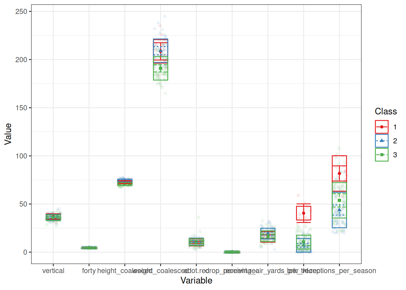
The tiers were not particularly distinguishable based on their height, weight, vertical jump, or forty-yard dash time.
Type 1 (“Elite/WR1”) WRs:
Type 2 (“Consistent Contributor/WR2”) WRs:
Type 3 (“Deep Threat/Boom-or-Bust”) WRs:
And here are the clusters based on the tidyLPA (Rosenberg et al., 2018; Rosenberg & van Lissa, 2021) solution:
Code
Code
                              [,1]   [,2]   [,3]
Class                         1.00   2.00   3.00
vertical                     36.93  36.42  35.78
forty                         4.46   4.50   4.43
height_coalesced             72.79  74.31  70.58
weight_coalesced            207.57 209.69 188.26
adot.rec                     10.21  11.04  10.51
drop_percent.rec              0.04   0.05   0.05
receiving_air_yards_per_rec  15.87  20.07  16.05
brk_tkl.rec                  42.71   7.76  10.04
receptions_per_season        81.01  44.17  51.43
type                          1.00   2.50   2.53
model_number                  3.00   3.00   3.00
classes_number                3.00   3.00   3.00
CPROB1                        0.93   0.00   0.00
CPROB2                        0.00   0.93   0.05
CPROB3                        0.07   0.07   0.94
21.2 Conclusion
The goal of cluster analysis is to identify distinguishable subgroups of people. There are many approaches to cluster analysis, including model-based clustering, density-based clustering, centroid-based clustering, hierarchical clustering (aka connectivity-based clustering), and others. The present chapter used model-based clustering to identify tiers of players based on projected points. Using various performance metrics of Wide Receivers, we identified three subtypes of Wide Receivers: 1) Elite WR1s who are strong possession receivers; 2) Consistent Contributor/WR2s; 3) deep threats/boom-or-bust receivers. The “Elite WR1s” tended to have the lowest drop percentage, the shortest average depth of target, the fewest receiving air yards per reception, the most receptions per season, and the most broken tackles. The “Consistent Contributor/WR2s” had fewer receptions and fewer broken tackles than the Elite WR1s; their average depth of target was longer than Elite WR1s, and they had more receiving air yards per reception than Elite WR1s. The “Deep Threat/Boom-or-Bust” receivers had the greatest average depth of target and the most receiving yards per reception; however, they also had the fewest receptions, the highest drop percentage, and the fewest broken tackles. In sum, cluster analysis can be a useful way of identifying subgroups of individuals who are more similar to one another on various characteristics.
21.3 Session Info
R version 4.6.1 (2026-06-24)
Platform: x86_64-pc-linux-gnu
Running under: Ubuntu 24.04.4 LTS

Matrix products: default
BLAS:   /usr/lib/x86_64-linux-gnu/openblas-pthread/libblas.so.3
LAPACK: /usr/lib/x86_64-linux-gnu/openblas-pthread/libopenblasp-r0.3.26.so;  LAPACK version 3.12.0

locale:
 [1] LC_CTYPE=C.UTF-8       LC_NUMERIC=C           LC_TIME=C.UTF-8
 [4] LC_COLLATE=C.UTF-8     LC_MONETARY=C.UTF-8    LC_MESSAGES=C.UTF-8
 [7] LC_PAPER=C.UTF-8       LC_NAME=C              LC_ADDRESS=C
[10] LC_TELEPHONE=C         LC_MEASUREMENT=C.UTF-8 LC_IDENTIFICATION=C

time zone: UTC
tzcode source: system (glibc)

attached base packages:
[1] stats     graphics  grDevices utils     datasets  methods   base

other attached packages:
 [1] lubridate_1.9.5   forcats_1.0.1     stringr_1.6.0     dplyr_1.2.1
 [5] purrr_1.2.2       readr_2.2.0       tidyr_1.3.2       tibble_3.3.1
 [9] tidyverse_2.0.0   plotly_4.12.0     ggplot2_4.0.3     tidyLPA_2.0.2
[13] tidySEM_0.2.10    mclust_6.1.3      nflreadr_1.5.1    petersenlab_1.2.3

loaded via a namespace (and not attached):
  [1] Rdpack_2.6.6        DBI_1.3.0           mnormt_2.1.2
  [4] gridExtra_2.3.1     sandwich_3.1-2      rlang_1.3.0
  [7] magrittr_2.0.5      otel_0.2.0          compiler_4.6.1
 [10] vctrs_0.7.3         reshape2_1.4.5      quadprog_1.5-8
 [13] crayon_1.5.3        pkgconfig_2.0.3     fastmap_1.2.0
 [16] backports_1.5.1     labeling_0.4.3      pbivnorm_0.6.0
 [19] pander_0.6.6        rmarkdown_2.31      tzdb_0.5.0
 [22] nloptr_2.2.1        xfun_0.60           cachem_1.1.0
 [25] jsonlite_2.0.0      progress_1.2.3      psych_2.6.5
 [28] prettyunits_1.2.0   parallel_4.6.1      lavaan_0.6-21
 [31] cluster_2.1.8.2     R6_2.6.1            stringi_1.8.7
 [34] RColorBrewer_1.1-3  parallelly_1.48.0   car_3.1-5
 [37] boot_1.3-32         rpart_4.1.27        Rcpp_1.1.2
 [40] knitr_1.51          future.apply_1.20.2 zoo_1.8-15
 [43] base64enc_0.1-6     timechange_0.4.0    Matrix_1.7-5
 [46] splines_4.6.1       nnet_7.3-20         igraph_2.3.3
 [49] tidyselect_1.2.1    rstudioapi_0.19.0   abind_1.4-8
 [52] yaml_2.3.12         codetools_0.2-20    listenv_1.0.0
 [55] lattice_0.22-9      nonnest2_0.5-9      plyr_1.8.9
 [58] withr_3.0.3         S7_0.2.2            coda_0.19-4.1
 [61] evaluate_1.0.5      foreign_0.8-91      future_1.70.0
 [64] fastDummies_1.7.6   CompQuadForm_1.4.4  texreg_1.39.5
 [67] pillar_1.11.1       carData_3.0-6       checkmate_2.3.4
 [70] stats4_4.6.1        reformulas_0.4.4    generics_0.1.4
 [73] dbscan_1.2.5        hms_1.1.4           mix_1.0-13
 [76] scales_1.4.0        minqa_1.2.8         globals_0.19.1
 [79] xtable_1.8-8        glue_1.8.1          lazyeval_0.2.3
 [82] Hmisc_5.2-6         tools_4.6.1         data.table_1.18.4
 [85] lme4_2.0-1          gsubfn_0.7          RANN_2.6.2
 [88] mvtnorm_1.4-2       grid_4.6.1          mitools_2.4
 [91] crosstalk_1.2.2     MplusAutomation_1.3 rbibutils_2.4.1
 [94] colorspace_2.1-3    nlme_3.1-169        htmlTable_2.5.0
 [97] proto_1.0.0         Formula_1.2-5       cli_3.6.6
[100] viridisLite_0.4.3   gtable_0.3.6        digest_0.6.39
[103] progressr_1.0.0     htmlwidgets_1.6.4   farver_2.1.2
[106] memoise_2.0.1       htmltools_0.5.9     lifecycle_1.0.5
[109] httr_1.4.8          MASS_7.3-65