I want your feedback to make the book better for you and other readers. If you find typos, errors, or places where the text may be improved, please let me know. The best ways to provide feedback are by GitHub or hypothes.is annotations.
You can leave a comment at the bottom of the page/chapter, or open an issue or submit a pull request on GitHub: https://github.com/isaactpetersen/Fantasy-Football-Analytics-Textbook
Alternatively, you can leave an annotation using hypothes.is.
To add an annotation, select some text and then click the
symbol on the pop-up menu.
To see the annotations of others, click the
symbol in the upper right-hand corner of the page.
25 Time Series Analysis
This chapter provides an overview of time series analysis.
25.1 Getting Started
25.1.1 Load Packages
25.1.2 Load Data
We created the player_stats_weekly.RData and player_stats_seasonal.RData objects in Section 4.4.3. The following code loads the Bayesian model object that was fit in Section 12.4.5.
25.2 Overview of Time Series Analysis
Time series analysis is useful when trying to generate forecasts from longitudinal data. That is, time series analysis seeks to evaluate change over time to predict future values.
There many different types of time series analyses. For simplicity, in this chapter, we use autoregressive integrated moving average (ARIMA) and exponential smoothing models to demonstrate one approach to time series analysis. We also leverage Bayesian mixed models to generate forecasts of future performance and plots of individuals model-implied performance by age and position.
There are four (potential) key components of time series data:
- seasonality
- trend
- cycle
- irregularity
Seasonality corresponds to fluctuations that occur at fixed and known periods (e.g., time of day, day of week, or month of year) (Hyndman & Athanasopoulos, 2021). A trend represents a long-term change (i.e., increase or decrease) in the series. A cycle reflects one or more rises and falls that are not of a fixed frequency, with durations typically lasting at least two years (Hyndman & Athanasopoulos, 2021). Irregularity is random variation or noise.
25.3 Autoregressive Integrated Moving Average (ARIMA) Models
Hyndman & Athanasopoulos (2021) provide a nice overview of ARIMA models. As noted by Hyndman & Athanasopoulos (2021), ARIMA models aim to describe how a variable is correlated with itself over time (autocorrelation)—i.e., how earlier levels of a variable are correlated with later levels of the same variable. ARIMA models perform best when there is a clear pattern where later values are influenced by earlier values. ARIMA models incorporate autoregression effects, moving average effects, and differencing.
ARIMA models can have various numbers of terms and model complexity. They are specified in the following form: \(\text{ARIMA}(p,d,q)\), where:
- \(p =\) the number of autoregressive terms
- \(d =\) the number of differences between consecutive scores (to make the time series stationary by reducing trends and seasonality)
- \(q =\) the number of moving average terms
ARIMA models assume that the data are stationary (i.e., there are no long-term trends), are non-seasonal (i.e., there is no consistency of the timing of the peaks or troughs in the line), and that earlier values influence later values. This may not strongly be the case in fantasy football, so ARIMA models may not be particularly useful in forecasting fantasy football performance. Other approaches, such as exponential smoothing, may be useful for data that show longer-term trends and seasonality (Hyndman & Athanasopoulos, 2021). Nevertheless, ARIMA models are widely used in forecasting financial markets and economic indicators. Thus, it is a useful technique to learn.
Adapted from: https://rc2e.com/timeseriesanalysis (Long & Teetor, 2019; archived at https://perma.cc/U5P6-2VWC).
25.3.1 Create the Time Series Objects
Code
weeklyFantasyPoints_tomBrady <- player_stats_weekly |>
filter(
player_id == "00-0019596" | player_display_name == "Tom Brady")
weeklyFantasyPoints_peytonManning <- player_stats_weekly |>
filter(
player_id == "00-0010346" | player_display_name == "Peyton Manning")
ts_tomBrady <- xts::xts(
x = weeklyFantasyPoints_tomBrady["fantasyPoints"],
order.by = weeklyFantasyPoints_tomBrady$gameday)
ts_peytonManning <- xts::xts(
x = weeklyFantasyPoints_peytonManning["fantasyPoints"],
order.by = weeklyFantasyPoints_peytonManning$gameday)
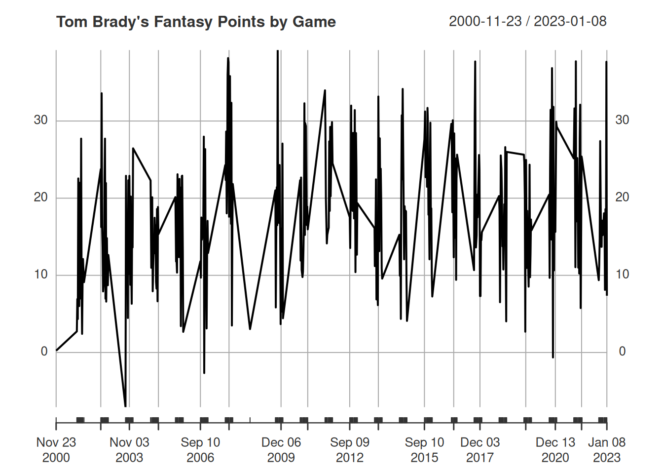
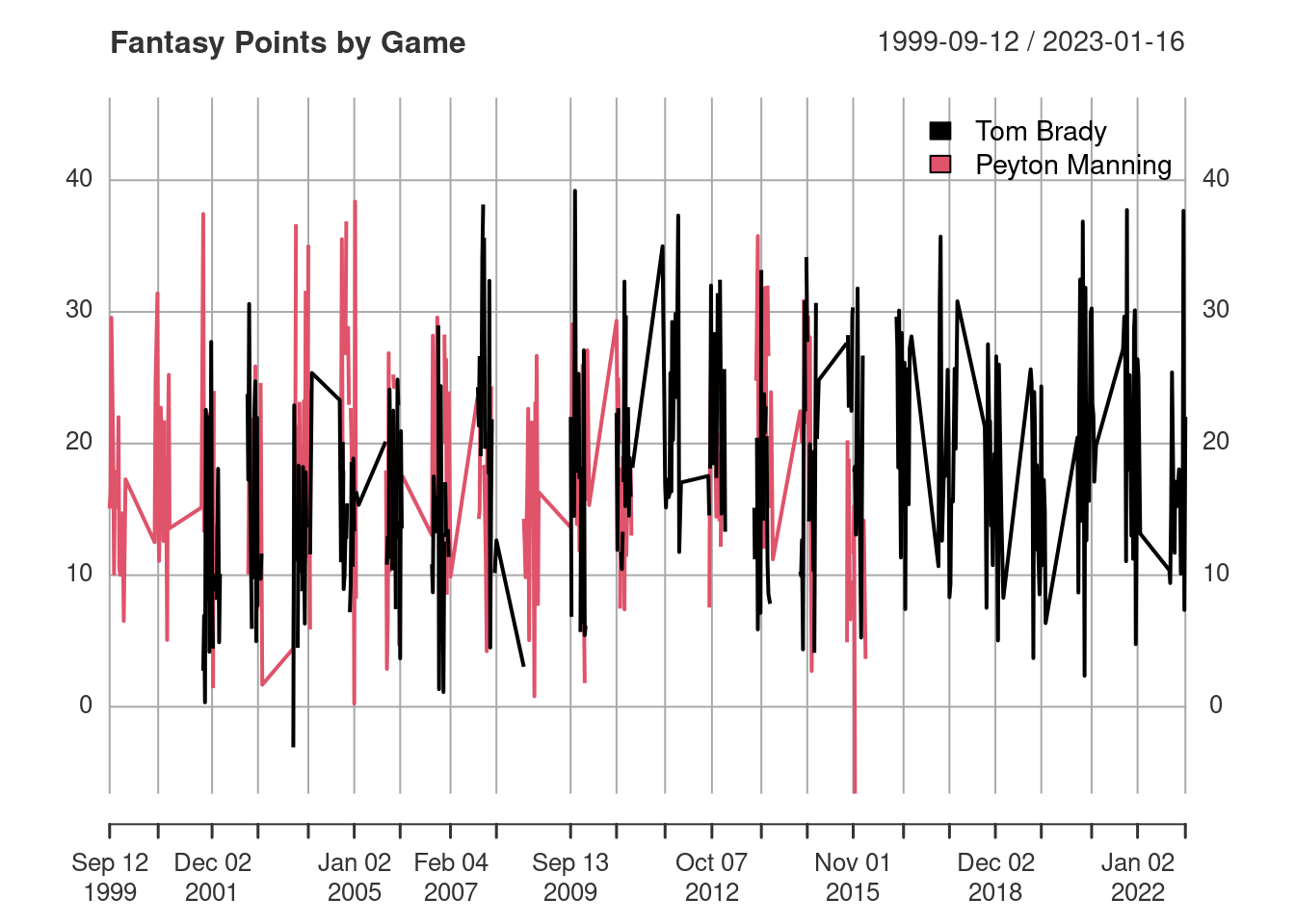
ts_tomBrady fantasyPoints
2000-11-23 0.24
2001-09-23 2.74
2001-09-30 6.92
2001-10-07 4.34
2001-10-14 22.56
2001-10-21 19.88
2001-10-28 10.02
2001-11-04 22.00
2001-11-11 8.18
2001-11-18 9.00
...
2022-10-27 17.10
2022-11-06 15.20
2022-11-13 17.02
2022-11-27 18.04
2022-12-05 17.14
2022-12-11 10.12
2022-12-18 20.58
2022-12-25 11.34
2023-01-01 37.68
2023-01-08 7.36 fantasyPoints
1999-09-12 15.06
1999-09-19 17.22
1999-09-26 29.56
1999-10-10 20.66
1999-10-17 10.10
1999-10-24 17.86
1999-10-31 18.52
1999-11-07 20.60
1999-11-14 15.18
1999-11-21 22.80
...
2015-09-13 4.90
2015-09-17 20.24
2015-09-27 18.86
2015-10-04 8.32
2015-10-11 6.64
2015-10-18 9.60
2015-11-01 11.60
2015-11-08 15.24
2015-11-15 -6.60
2016-01-03 2.5625.3.2 Plot the Time Series
25.3.3 Rolling Mean/Median
fantasyPoints
2001-09-30 7.360
2001-10-07 11.288
2001-10-14 12.744
2001-10-21 15.760
2001-10-28 16.528
2001-11-04 13.816
2001-11-11 15.384
2001-11-18 15.084
2001-11-25 11.568
2001-12-02 11.888
...
2022-10-16 18.332
2022-10-23 15.892
2022-10-27 15.348
2022-11-06 16.212
2022-11-13 16.900
2022-11-27 15.504
2022-12-05 16.580
2022-12-11 15.444
2022-12-18 19.372
2022-12-25 17.416 fantasyPoints
2001-09-30 4.34
2001-10-07 6.92
2001-10-14 10.02
2001-10-21 19.88
2001-10-28 19.88
2001-11-04 10.02
2001-11-11 10.02
2001-11-18 9.00
2001-11-25 8.52
2001-12-02 9.00
...
2022-10-16 17.10
2022-10-23 15.20
2022-10-27 15.20
2022-11-06 17.02
2022-11-13 17.10
2022-11-27 17.02
2022-12-05 17.14
2022-12-11 17.14
2022-12-18 17.14
2022-12-25 11.3425.3.4 Autocorrelation
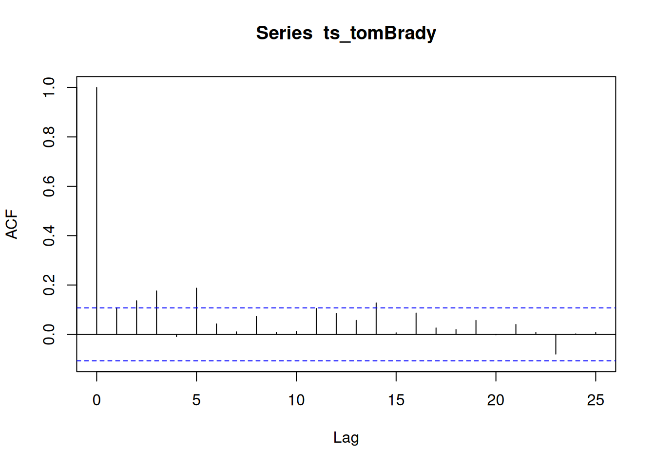
The autocorrelation function (ACF) plot depicts the autocorrelation of scores as a function of the length of the lag. We can generate an ACF plot using the stats::acf() function. Significant autocorrelation is detected when the autocorrelation exceeds the dashed blue lines, as is depicted in Figure 25.3.
25.3.5 Fit an Autoregressive Integrated Moving Average Model
We can fit an ARIMA model using the forecast::auto.arima() function of the forecast package (Hyndman et al., 2024; Hyndman & Khandakar, 2008):
Series: ts_tomBrady
ARIMA(2,1,2)
Coefficients:
ar1 ar2 ma1 ma2
0.5827 0.0703 -1.5041 0.5161
s.e. 0.2615 0.0658 0.2577 0.2496
sigma^2 = 62.76: log likelihood = -1164.4
AIC=2338.8 AICc=2338.99 BIC=2357.86Series: ts_peytonManning
ARIMA(1,0,1) with non-zero mean
Coefficients:
ar1 ma1 mean
0.8659 -0.7311 18.1529
s.e. 0.0973 0.1287 0.9575
sigma^2 = 57.94: log likelihood = -860.72
AIC=1729.43 AICc=1729.59 BIC=1743.52We can generate a plot of an ARIMA model using the stats::arima() function.
Call:
arima(x = ts_tomBrady, order = c(5, 1, 4))
Coefficients: ar1 ar2 ar3 ar4 ar5 ma1 ma2 ma3
0.3416 -0.0655 -0.205 -0.0959 0.1961 -1.2442 0.3689 0.2403
s.e. NaN 0.2256 NaN 0.0475 0.0571 NaN NaN NaN
ma4
-0.3361
s.e. NaN
sigma^2 estimated as 59.78: log likelihood = -1158.36, aic = 2336.72
Training set error measures:
ME RMSE MAE MPE MAPE MASE
Training set 0.6879023 7.720194 6.223572 -21.21763 50.46479 0.732154
ACF1
Training set -0.0007899074 2.5 % 97.5 %
ar1 NaN NaN
ar2 -0.50779428 0.376718457
ar3 NaN NaN
ar4 -0.18900813 -0.002859993
ar5 0.08427103 0.307929276
ma1 NaN NaN
ma2 NaN NaN
ma3 NaN NaN
ma4 NaN NaN
Ljung-Box test
data: Residuals from ARIMA(5,1,4)
Q* = 4.3247, df = 3, p-value = 0.2285
Model df: 9. Total lags used: 12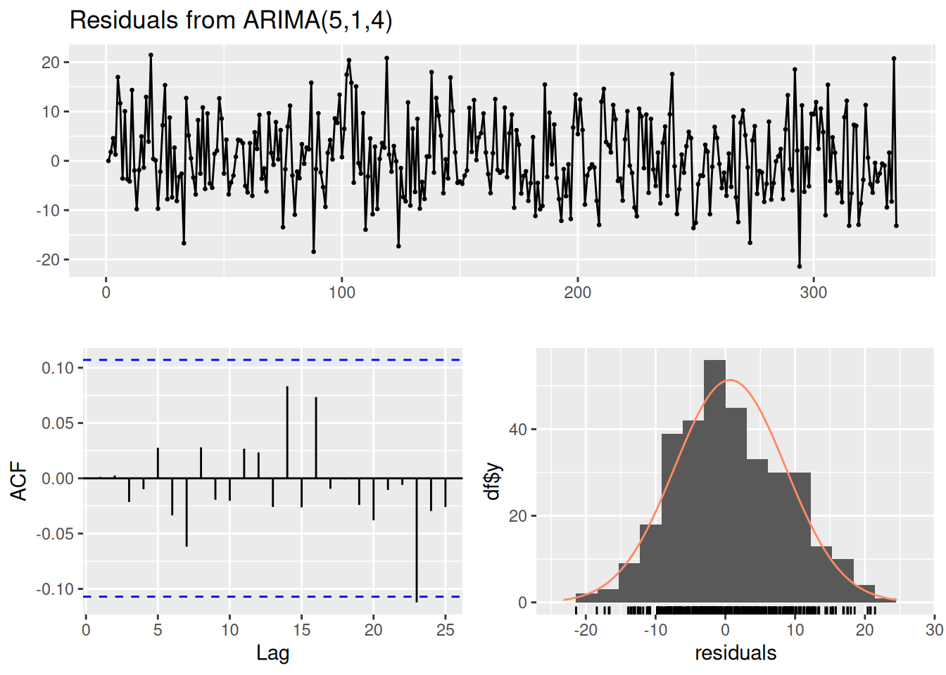
Code
Call:
arima(x = ts_tomBrady, order = c(5, 1, 4), fixed = c(NA, NA, 0, NA, NA, NA,
NA, NA, NA))
Coefficients:
ar1 ar2 ar3 ar4 ar5 ma1 ma2 ma3 ma4
-0.9051 -0.7933 0 0.0987 0.1551 0.0137 -0.0185 -0.6539 -0.2529
s.e. 0.3144 0.1769 0 0.1013 0.0929 0.3217 0.2181 0.1528 0.1079
sigma^2 estimated as 59.38: log likelihood = -1157.29, aic = 2332.58
Training set error measures:
ME RMSE MAE MPE MAPE MASE
Training set 0.6609654 7.694434 6.168512 -20.93448 50.25172 0.7256766
ACF1
Training set -0.006363576 2.5 % 97.5 %
ar1 -1.52137219 -0.28875955
ar2 -1.13999746 -0.44652063
ar3 NA NA
ar4 -0.09983263 0.29728144
ar5 -0.02703935 0.33727487
ma1 -0.61686843 0.64426701
ma2 -0.44596328 0.40905685
ma3 -0.95344054 -0.35438261
ma4 -0.46435785 -0.04145554
Ljung-Box test
data: Residuals from ARIMA(5,1,4)
Q* = 3.3999, df = 3, p-value = 0.334
Model df: 9. Total lags used: 12
Code
Call:
arima(x = ts_peytonManning, order = c(1, 0, 1))
Coefficients:
ar1 ma1 intercept
0.8659 -0.7311 18.1529
s.e. 0.0973 0.1287 0.9575
sigma^2 estimated as 57.24: log likelihood = -860.72, aic = 1729.43
Training set error measures:
ME RMSE MAE MPE MAPE MASE
Training set 0.002008698 7.565751 5.932631 -101.5589 126.2153 0.7578856
ACF1
Training set 0.02467125 2.5 % 97.5 %
ar1 0.6752778 1.0565343
ma1 -0.9833206 -0.4789367
intercept 16.2763161 20.0295532
Ljung-Box test
data: Residuals from ARIMA(1,0,1) with non-zero mean
Q* = 9.7829, df = 8, p-value = 0.2806
Model df: 2. Total lags used: 10
25.3.6 Generate the Model Forecasts
We can generate model forecasts from the ARIMA model using the forecast::forecast() function.
Code
Point Forecast Lo 80 Hi 80 Lo 95 Hi 95
336 16.89941 6.990778 26.80803 1.7454680 32.05334
337 21.84148 11.885926 31.79704 6.6157730 37.06719
338 14.62678 4.629175 24.62438 -0.6632356 29.91679
339 22.63793 12.473318 32.80254 7.0924968 38.18336
340 17.97384 7.804932 28.14275 2.4218376 33.52584
341 18.73072 8.416107 29.04533 2.9558825 34.50555
342 19.31420 8.980909 29.64748 3.5107975 35.11759
343 18.23659 7.893548 28.57964 2.4182709 34.05491
344 19.69349 9.341389 30.04559 3.8613185 35.52566
345 19.15502 8.802780 29.50726 3.3226357 34.98740 Point Forecast Lo 80 Hi 80 Lo 95 Hi 95
251 12.03144 2.335537 21.72734 -2.79716238 26.86004
252 12.85229 3.068726 22.63586 -2.11038095 27.81497
253 13.56308 3.714290 23.41186 -1.49934216 28.62550
254 14.17855 4.281143 24.07595 -0.95822712 29.31533
255 14.71149 4.777786 24.64519 -0.48079979 29.90378
256 15.17297 5.212133 25.13380 -0.06081402 30.40675
257 15.57256 5.591435 25.55369 0.30774583 30.83738
258 15.91857 5.922259 25.91489 0.63052902 31.20662
259 16.21819 6.210500 26.22588 0.91274926 31.52363
260 16.47763 6.461418 26.49383 1.15915808 31.7961025.3.7 Plot the Model Forecasts
We can plot the model forecasts using the forecast::autoplot() function.
Code
Code
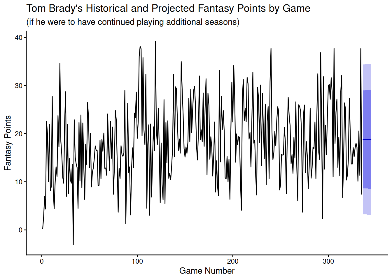
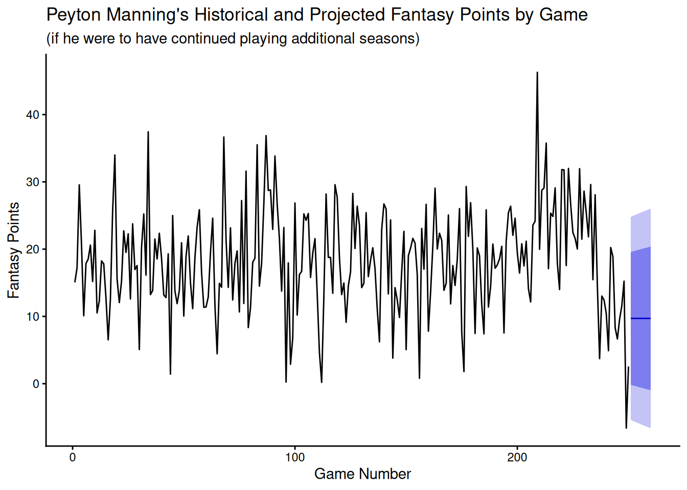
25.4 Exponential Smoothing
25.4.1 Fit the Exponential Smoothing Model
We fit exponential smoothing models using the forecast::ets() function of the forecast package (Hyndman et al., 2024; Hyndman & Khandakar, 2008):
We can generate a plot of an ARIMA model using the stats::arima() function.
ETS(A,N,N)
Call:
forecast::ets(y = ts_tomBrady)
Smoothing parameters:
alpha = 0.0426
Initial states:
l = 13.5319
sigma: 7.9439
AIC AICc BIC
3340.243 3340.315 3351.685
Training set error measures:
ME RMSE MAE MPE MAPE MASE ACF1
Training set 0.3709126 7.9202 6.376596 -42.104 70.03779 0.7501561 0.04152263
Ljung-Box test
data: Residuals from ETS(A,N,N)
Q* = 19.391, df = 10, p-value = 0.03557
Model df: 0. Total lags used: 10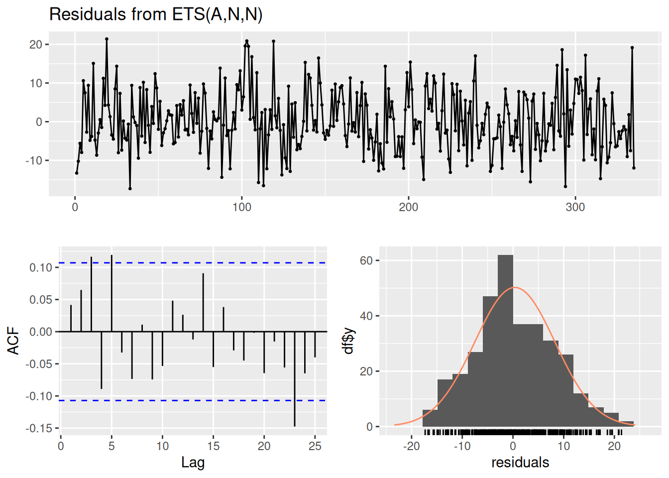
ETS(A,N,N)
Call:
forecast::ets(y = ts_peytonManning)
Smoothing parameters:
alpha = 0.1375
Initial states:
l = 18.0175
sigma: 7.7031
AIC AICc BIC
2405.168 2405.266 2415.733
Training set error measures:
ME RMSE MAE MPE MAPE MASE
Training set -0.2418607 7.672223 6.032439 -107.9247 132.1507 0.770636
ACF1
Training set 0.04883502
Ljung-Box test
data: Residuals from ETS(A,N,N)
Q* = 11.003, df = 10, p-value = 0.3573
Model df: 0. Total lags used: 10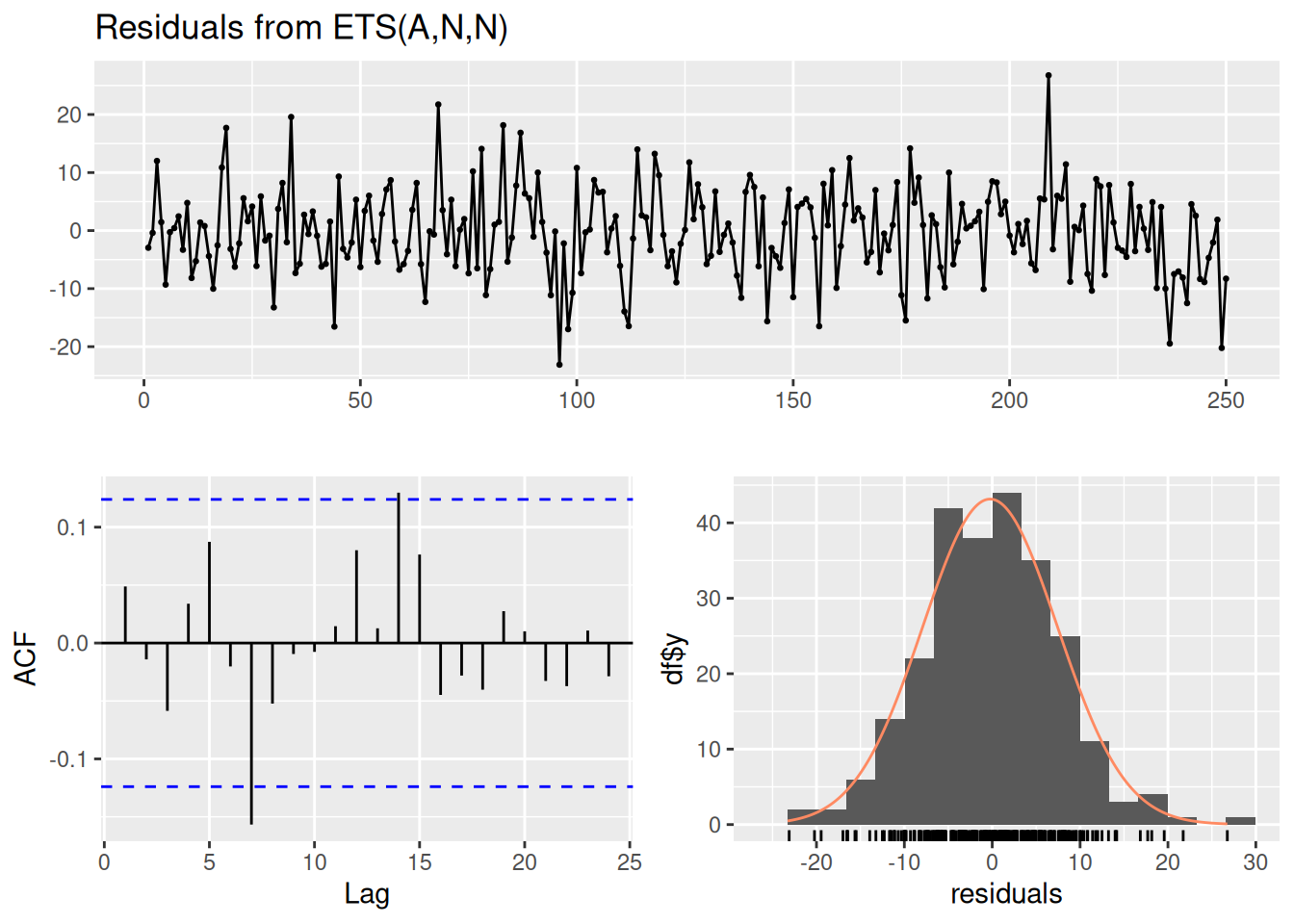
25.4.2 Generate the Model Forecasts
We can generate model forecasts from the ARIMA model using the forecast::forecast() function.
Code
Point Forecast Lo 80 Hi 80 Lo 95 Hi 95
336 18.82671 8.646134 29.00729 3.256861 34.39657
337 18.82671 8.636896 29.01653 3.242732 34.41070
338 18.82671 8.627666 29.02576 3.228615 34.42481
339 18.82671 8.618444 29.03499 3.214512 34.43892
340 18.82671 8.609230 29.04420 3.200421 34.45301
341 18.82671 8.600025 29.05340 3.186342 34.46709
342 18.82671 8.590828 29.06260 3.172277 34.48115
343 18.82671 8.581639 29.07179 3.158224 34.49521
344 18.82671 8.572459 29.08097 3.144183 34.50925
345 18.82671 8.563286 29.09014 3.130156 34.52327 Point Forecast Lo 80 Hi 80 Lo 95 Hi 95
251 9.705069 -0.1668464 19.57699 -5.392723 24.80286
252 9.705069 -0.2596969 19.66984 -5.534726 24.94486
253 9.705069 -0.3516901 19.76183 -5.675417 25.08556
254 9.705069 -0.4428494 19.85299 -5.814833 25.22497
255 9.705069 -0.5331971 19.94334 -5.953008 25.36315
256 9.705069 -0.6227545 20.03289 -6.089974 25.50011
257 9.705069 -0.7115419 20.12168 -6.225763 25.63590
258 9.705069 -0.7995789 20.20972 -6.360404 25.77054
259 9.705069 -0.8868841 20.29702 -6.493926 25.90406
260 9.705069 -0.9734757 20.38361 -6.626356 26.0364925.4.3 Plot the Model Forecasts
We can plot the model forecasts using the forecast::autoplot() function.
Code
Code
25.5 Bayesian Mixed Models
The Bayesian longitudinal mixed models were estimated in Section 12.4.5.
25.5.1 Prepare New Data Object
Code
player_stats_seasonal_offense_subset <- player_stats_seasonal |>
dplyr::filter(position_group %in% c("QB","RB","WR","TE") | position %in% c("K"))
player_stats_seasonal_offense_subset$position[which(player_stats_seasonal_offense_subset$position == "HB")] <- "RB"
player_stats_seasonal_offense_subset$player_idFactor <- factor(player_stats_seasonal_offense_subset$player_id)
player_stats_seasonal_offense_subset$positionFactor <- factor(player_stats_seasonal_offense_subset$position)Code
player_stats_seasonal_offense_subsetCC <- player_stats_seasonal_offense_subset |>
filter(
!is.na(player_idFactor),
!is.na(fantasyPoints),
!is.na(positionFactor),
!is.na(ageCentered20),
!is.na(ageCentered20Quadratic),
!is.na(years_of_experience))
player_stats_seasonal_offense_subsetCC <- player_stats_seasonal_offense_subsetCC |>
filter(player_id %in% bayesianMixedModelFit$data$player_idFactor) |>
mutate(positionFactor = droplevels(positionFactor))
player_stats_seasonal_offense_subsetCC <- player_stats_seasonal_offense_subsetCC |>
group_by(player_id) |>
group_modify(~ add_row(.x, season = max(player_stats_seasonal_offense_subsetCC$season) + 1)) |>
fill(player_display_name, player_idFactor, position, position_group, positionFactor, team, .direction = "downup") |>
ungroup()
player_stats_seasonal_offense_subsetCC <- player_stats_seasonal_offense_subsetCC |>
left_join(
player_stats_seasonal_offense_subsetCC |>
filter(season == max(player_stats_seasonal_offense_subsetCC$season) - 1) |>
select(player_id, age_lastYear = age, years_of_experience_lastYear = years_of_experience),
by = "player_id") |>
mutate(
age = if_else(season == max(player_stats_seasonal_offense_subsetCC$season), age_lastYear + 1, age), # increment age by 1
ageCentered20 = age - 20,
years_of_experience = if_else(season == max(player_stats_seasonal_offense_subsetCC$season), years_of_experience_lastYear + 1, years_of_experience)) # increment experience by 1
activePlayers <- unique(player_stats_seasonal_offense_subsetCC[c("player_id","season")]) |>
filter(season == max(player_stats_seasonal_offense_subsetCC$season) - 1) |>
select(player_id) |>
pull()
inactivePlayers <- player_stats_seasonal_offense_subsetCC$player_id[which(player_stats_seasonal_offense_subsetCC$player_id %ni% activePlayers)]
player_stats_seasonal_offense_subsetCC <- player_stats_seasonal_offense_subsetCC |>
filter(player_id %in% activePlayers | (player_id %in% inactivePlayers & season < max(player_stats_seasonal_offense_subsetCC$season) - 1)) |>
mutate(
player_idFactor = droplevels(player_idFactor)
)25.5.2 Generate Predictions
25.5.3 Table of Next Season Predictions
Code
Code
Code
Code
25.5.4 Plot of Individuals’ Model-Implied Predictions
25.5.4.1 Quarterbacks
Code
plot_individualFantasyPointsByAgeQB <- ggplot(
data = player_stats_seasonal_offense_subsetCC |> filter(position == "QB"),
mapping = aes(
x = round(age, 2),
y = round(fantasyPoints_bayesian, 2),
group = player_id)) +
geom_smooth(
aes(
x = age,
y = fantasyPoints_bayesian,
text = player_display_name, # add player name for mouse over tooltip
label = season # add season for mouse over tooltip
),
se = FALSE,
linewidth = 0.5,
color = "black") +
geom_point(
aes(
x = age,
y = fantasyPoints_bayesian,
text = player_display_name, # add player name for mouse over tooltip
label = season # add season for mouse over tooltip
),
size = 1,
color = "transparent" # make points invisible but keep tooltips
) +
labs(
x = "Player Age (years)",
y = "Fantasy Points (Season)",
title = "Fantasy Points (Season) by Player Age: Quarterbacks"
) +
theme_classic()
plotly::ggplotly(
plot_individualFantasyPointsByAgeQB,
tooltip = c("age","fantasyPoints_bayesian","text","label")
)25.5.4.2 Running Backs
Code
plot_individualFantasyPointsByAgeRB <- ggplot(
data = player_stats_seasonal_offense_subsetCC |> filter(position == "RB"),
mapping = aes(
x = age,
y = fantasyPoints_bayesian,
group = player_id)) +
geom_smooth(
aes(
x = age,
y = fantasyPoints_bayesian,
text = player_display_name, # add player name for mouse over tooltip
label = season # add season for mouse over tooltip
),
se = FALSE,
linewidth = 0.5,
color = "black") +
geom_point(
aes(
x = age,
y = fantasyPoints_bayesian,
text = player_display_name, # add player name for mouse over tooltip
label = season # add season for mouse over tooltip
),
size = 1,
color = "transparent" # make points invisible but keep tooltips
) +
labs(
x = "Player Age (years)",
y = "Fantasy Points (Season)",
title = "Fantasy Points (Season) by Player Age: Running Backs"
) +
theme_classic()
plotly::ggplotly(
plot_individualFantasyPointsByAgeRB,
tooltip = c("age","fantasyPoints_bayesian","text","label")
)25.5.4.3 Wide Receivers
Code
plot_individualFantasyPointsByAgeWR <- ggplot(
data = player_stats_seasonal_offense_subsetCC |> filter(position == "WR"),
mapping = aes(
x = age,
y = fantasyPoints_bayesian,
group = player_id)) +
geom_smooth(
aes(
x = age,
y = fantasyPoints_bayesian,
text = player_display_name, # add player name for mouse over tooltip
label = season # add season for mouse over tooltip
),
se = FALSE,
linewidth = 0.5,
color = "black") +
geom_point(
aes(
x = age,
y = fantasyPoints_bayesian,
text = player_display_name, # add player name for mouse over tooltip
label = season # add season for mouse over tooltip
),
size = 1,
color = "transparent" # make points invisible but keep tooltips
) +
labs(
x = "Player Age (years)",
y = "Fantasy Points (Season)",
title = "Fantasy Points (Season) by Player Age: Wide Receivers"
) +
theme_classic()
plotly::ggplotly(
plot_individualFantasyPointsByAgeWR,
tooltip = c("age","fantasyPoints_bayesian","text","label")
)25.5.4.4 Tight Ends
Code
plot_individualFantasyPointsByAgeTE <- ggplot(
data = player_stats_seasonal_offense_subsetCC |> filter(position == "TE"),
mapping = aes(
x = age,
y = fantasyPoints_bayesian,
group = player_id)) +
geom_smooth(
aes(
x = age,
y = fantasyPoints_bayesian,
text = player_display_name, # add player name for mouse over tooltip
label = season # add season for mouse over tooltip
),
se = FALSE,
linewidth = 0.5,
color = "black") +
geom_point(
aes(
x = age,
y = fantasyPoints_bayesian,
text = player_display_name, # add player name for mouse over tooltip
label = season # add season for mouse over tooltip
),
size = 1,
color = "transparent" # make points invisible but keep tooltips
) +
labs(
x = "Player Age (years)",
y = "Fantasy Points (Season)",
title = "Fantasy Points (Season) by Player Age: Tight Ends"
) +
theme_classic()
plotly::ggplotly(
plot_individualFantasyPointsByAgeTE,
tooltip = c("age","fantasyPoints_bayesian","text","label")
)25.6 Conclusion
That is, time series analysis seeks to evaluate change over time to predict future values. There many different types of time series analyses. We demonstrated use of autoregressive integrated moving average (ARIMA) models to predict future fantasy points. ARIMA models aim to describe how how earlier levels of a variable are correlated with later levels of the same variable. ARIMA models perform best when there is a clear pattern where later values are influenced by earlier values. ARIMA models assume that the data are stationary (i.e., there are no long-term trends), are non-seasonal (i.e., there is no consistency of the timing of the peaks or troughs in the line), and that earlier values influence later values. This may not strongly be the case in fantasy football, so ARIMA models may not be particularly useful in forecasting fantasy football performance. We also used Bayesian mixed models to generate forecasts of future performance and plots of individuals model-implied performance by age and position.
25.7 Session Info
R version 4.6.1 (2026-06-24)
Platform: x86_64-pc-linux-gnu
Running under: Ubuntu 24.04.4 LTS
Matrix products: default
BLAS: /usr/lib/x86_64-linux-gnu/openblas-pthread/libblas.so.3
LAPACK: /usr/lib/x86_64-linux-gnu/openblas-pthread/libopenblasp-r0.3.26.so; LAPACK version 3.12.0
locale:
[1] LC_CTYPE=C.UTF-8 LC_NUMERIC=C LC_TIME=C.UTF-8
[4] LC_COLLATE=C.UTF-8 LC_MONETARY=C.UTF-8 LC_MESSAGES=C.UTF-8
[7] LC_PAPER=C.UTF-8 LC_NAME=C LC_ADDRESS=C
[10] LC_TELEPHONE=C LC_MEASUREMENT=C.UTF-8 LC_IDENTIFICATION=C
time zone: UTC
tzcode source: system (glibc)
attached base packages:
[1] stats graphics grDevices utils datasets methods base
other attached packages:
[1] lubridate_1.9.5 forcats_1.0.1 stringr_1.6.0
[4] dplyr_1.2.1 purrr_1.2.2 readr_2.2.0
[7] tidyr_1.3.2 tibble_3.3.1 tidyverse_2.0.0
[10] plotly_4.12.1 ggplot2_4.0.3 rstan_2.32.7
[13] StanHeaders_2.32.10 brms_2.23.0 Rcpp_1.1.2
[16] forecast_9.0.2 xts_0.14.2 zoo_1.8-15
[19] petersenlab_1.2.3
loaded via a namespace (and not attached):
[1] RColorBrewer_1.1-3 tensorA_0.36.2.1 rstudioapi_0.19.0
[4] jsonlite_2.0.0 magrittr_2.0.5 TH.data_1.1-5
[7] estimability_2.0.0 farver_2.1.2 nloptr_2.2.1
[10] rmarkdown_2.31 vctrs_0.7.3 minqa_1.2.8
[13] base64enc_0.1-6 htmltools_0.5.9 distributional_0.8.1
[16] curl_7.1.0 Formula_1.2-5 htmlwidgets_1.6.4
[19] plyr_1.8.9 sandwich_3.1-2 emmeans_2.0.4
[22] lifecycle_1.0.5 pkgconfig_2.0.3 Matrix_1.7-5
[25] R6_2.6.1 fastmap_1.2.0 rbibutils_2.4.1
[28] digest_0.6.39 colorspace_2.1-3 ps_1.9.3
[31] crosstalk_1.2.2 Hmisc_5.2-6 labeling_0.4.3
[34] timechange_0.4.0 httr_1.4.8 abind_1.4-8
[37] mgcv_1.9-4 compiler_4.6.1 withr_3.0.3
[40] htmlTable_2.5.0 S7_0.2.2 backports_1.5.1
[43] inline_0.3.21 DBI_1.3.0 psych_2.6.5
[46] QuickJSR_1.10.0 pkgbuild_1.4.8 MASS_7.3-65
[49] loo_2.10.0 tools_4.6.1 pbivnorm_0.6.0
[52] foreign_0.8-91 otel_0.2.0 nnet_7.3-20
[55] glue_1.8.1 quadprog_1.5-8 nlme_3.1-169
[58] grid_4.6.1 cmdstanr_0.9.0.9001 checkmate_2.3.4
[61] cluster_2.1.8.2 reshape2_1.4.5 generics_0.1.4
[64] gtable_0.3.6 tzdb_0.5.0 data.table_1.18.4
[67] hms_1.1.4 pillar_1.11.1 posterior_1.7.0
[70] mitools_2.4 splines_4.6.1 lattice_0.22-9
[73] survival_3.8-6 tidyselect_1.2.1 mix_1.0-13
[76] knitr_1.51 reformulas_0.4.4 gridExtra_2.3.1
[79] V8_8.2.0 urca_1.3-4 stats4_4.6.1
[82] xfun_0.60 bridgesampling_1.2-1 timeDate_4052.112
[85] matrixStats_1.5.0 stringi_1.8.7 yaml_2.3.12
[88] boot_1.3-32 evaluate_1.0.5 codetools_0.2-20
[91] cli_3.6.6 RcppParallel_6.0.0 rpart_4.1.27
[94] xtable_1.8-8 Rdpack_2.6.6 processx_3.9.0
[97] lavaan_0.7-2 coda_0.19-4.1 parallel_4.6.1
[100] rstantools_2.6.0 fracdiff_1.5-4 bayesplot_1.15.0
[103] Brobdingnag_1.2-9 lme4_2.0-6 viridisLite_0.4.3
[106] mvtnorm_1.4-2 scales_1.4.0 rlang_1.3.0
[109] multcomp_1.4-31 mnormt_2.1.2