I want your feedback to make the book better for you and other readers. If you find typos, errors, or places where the text may be improved, please let me know.
The best ways to provide feedback are by GitHub or hypothes.is annotations.
Alternatively, you can leave an annotation using hypothes.is.
To add an annotation, select some text and then click the
symbol on the pop-up menu.
To see the annotations of others, click the
symbol in the upper right-hand corner of the page.
11Multiple Regression
This chapter provides an overview of multiple regression.
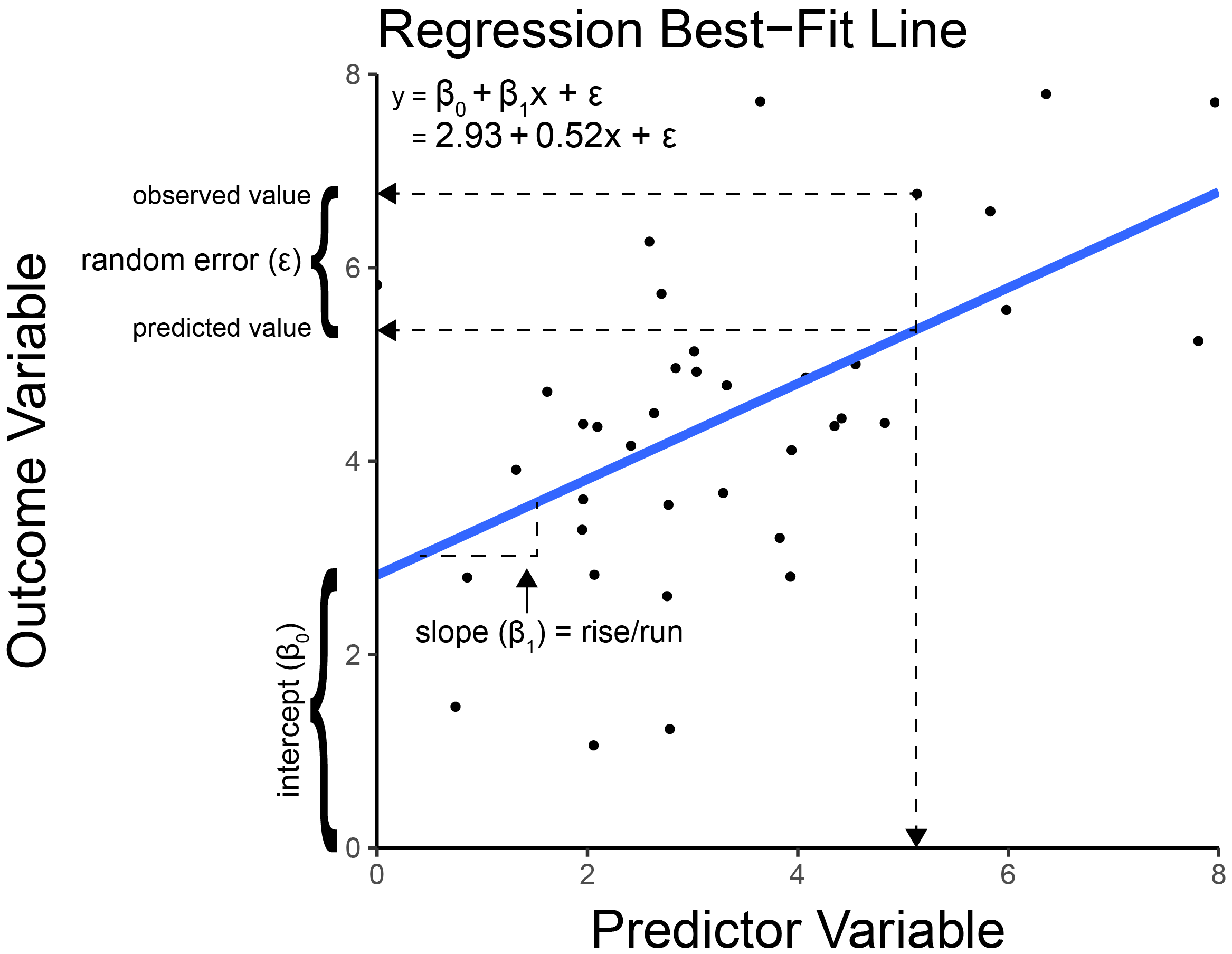
In multiple regression, we estimate models. A model is a simplification of reality. All statistical analyses follow the same basic structure, as in Equation 11.1:
\[
y = \beta_0 + \beta_1x_1 + \epsilon
\tag{11.2}\]
where \(y\) is the outcome variable, \(\beta_0\) is the intercept, \(\beta_1\) is the slope, \(x_1\) is the predictor variable, and \(\epsilon\) is the error term.
where \(p\) is the number of predictor variables. Multiple regression is basically a weighted sum of the predictor variables, and adding an intercept. Under the hood, multiple regression seeks to identify the best weight for each predictor. That is, multiple regression identifies the optimal linear combination of the predictor variables that explains the most variance in the outcome variable. The intercept is the expected value of the outcome variable when all of the predictor variables have a value of zero.
11.3 Components
\(B\) = unstandardized coefficient: direction and magnitude of the estimate (original scale)
\(\beta\) (beta) = standardized coefficient: direction and magnitude of the estimate (standard deviation scale)
\(SE\) = standard error: uncertainty of unstandardized estimate
\[
\text{unstandardized regression coefficient} = \frac{\text{unique covariance of } X \text{ with } Y}{\text{unique variance of X}}
\tag{11.5}\]
The unstandardized regression coefficient (\(B\)) is interpreted such that, for every unit change in the predictor variable, there is a __ unit change in the outcome variable (holding all other predictor variables constant). For instance, when examining the association between age and fantasy points, if the unstandardized regression coefficient is 2.3, players score on average 2.3 more points for each additional year of age. (In reality, we might expect a nonlinear, inverted-U-shaped association between age and fantasy points such that players tend to reach their peak in the middle of their careers.) Unstandardized regression coefficients are tied to the metric of the raw data. Thus, a large unstandardized regression coefficient for two variables may mean completely different things. Holding the strength of the association constant, you tend to see larger unstandardized regression coefficients for variables with smaller units and smaller unstandardized regression coefficients for variables with larger units.
11.3.2 Standardized Regression Coefficient
The standardized regression coefficient is computed as in Equation 11.6:
\[
\small
\text{standardized regression coefficient} = \text{unstandardized regression coefficient} \cdot \frac{\text{standard deviation of }X}{\text{standard deviation of }Y}
\tag{11.6}\]
Standardized regression coefficients can be obtained by standardizing the variables to z scores so they all have a mean of zero and standard deviation of one. The standardized regression coefficient (\(\beta\)) is interpreted such that, for every standard deviation change in the predictor variable, there is a __ standard deviation change in the outcome variable (holding all other predictor variables constant). For instance, when examining the association between age and fantasy points, if the standardized regression coefficient is 0.1, players score on average 0.1 standard deviation more points for each additional standard deviation of their year of age. Standardized regression coefficients—though not the case in all instances—tend to fall between [−1, 1]. Thus, standardized regression coefficients tend to be more comparable across variables and models compared to unstandardized regression coefficients. In this way, standardized regression coefficients provide a meaningful index of effect size and can be used to identify the predictors with the strongest predictive validity.
11.3.3 Standard Error
The standard error of a regression coefficient represents the imprecision or uncertainty of the parameter. If we have less uncertainty (i.e., more confidence) about the parameter, the standard error will be small, reflecting greater precision of the regression coefficient. If we have more uncertainty (i.e., less confidence) about the parameter, the standard error will be large, reflecting less precision of the regression coefficient. If we used the same sampling procedure repeatedly and calculated the regression coefficient each time, the true parameter in the population would fall 68% of the time within the interval of: \([\text{model parameter estimate for the regression coefficient} \pm 1 \text{ standard error}]\). The standard error is related to the sample size—the larger the sample size, the smaller the standard error (the greater the precision of our estimate of the regression coefficient). Otherwise said, having more data gives more precise estimates and thus increases statistical power.
11.3.4 Confidence Interval
A confidence interval represents a range of plausible values for a parameter, constructed so that, with repeated sampling, the intervals contain the true value with a specified long-run frequency (e.g., 95%). Our parameter estimate for the regression coefficient, plus or minus 1 standard error, reflects the 68% confidence interval for the coefficient. The 95% confidence interval is computed as the parameter estimate plus or minus 1.96 standard errors (because in a standard normal distribution, the middle 95% of the distribution lies between −1.96 and +1.96). For instance, if the parameter estimate for the regression coefficient is 0.50, and the standard error is 0.10, the 95% confidence interval is [0.30, 0.70]: \(0.5 - (1.96 \times 0.10) = 0.3\); \(0.5 + (1.96 \times 0.10) = 0.7\). That is, if we used the same sampling procedure repeatedly, about 95% of the confidence intervals (computed as parameter estimate \(\pm 1.959964 \ \text{standard errors}\)) would contain the true value of the regression coefficient.
We fit a (Bayesian) zero-one-inflated beta regression model (to allow for zeros and ones) using the brms::brm() function of the brms package (Bürkner, 2024) and specifying family = zero_one_inflated_beta().
Note 11.1: Bayesian beta regression
Note: the following code that runs the model takes a while. If you just want to save time and load the model object instead of running the model, you can load the model object (which has already been fit) using this code:
there is homoscedasticity of the residuals; the residuals do not differ as a function of the predictor variable or as a function of the outcome variable
the residuals are independent; they are uncorrelated with each other
the residuals are normally distributed
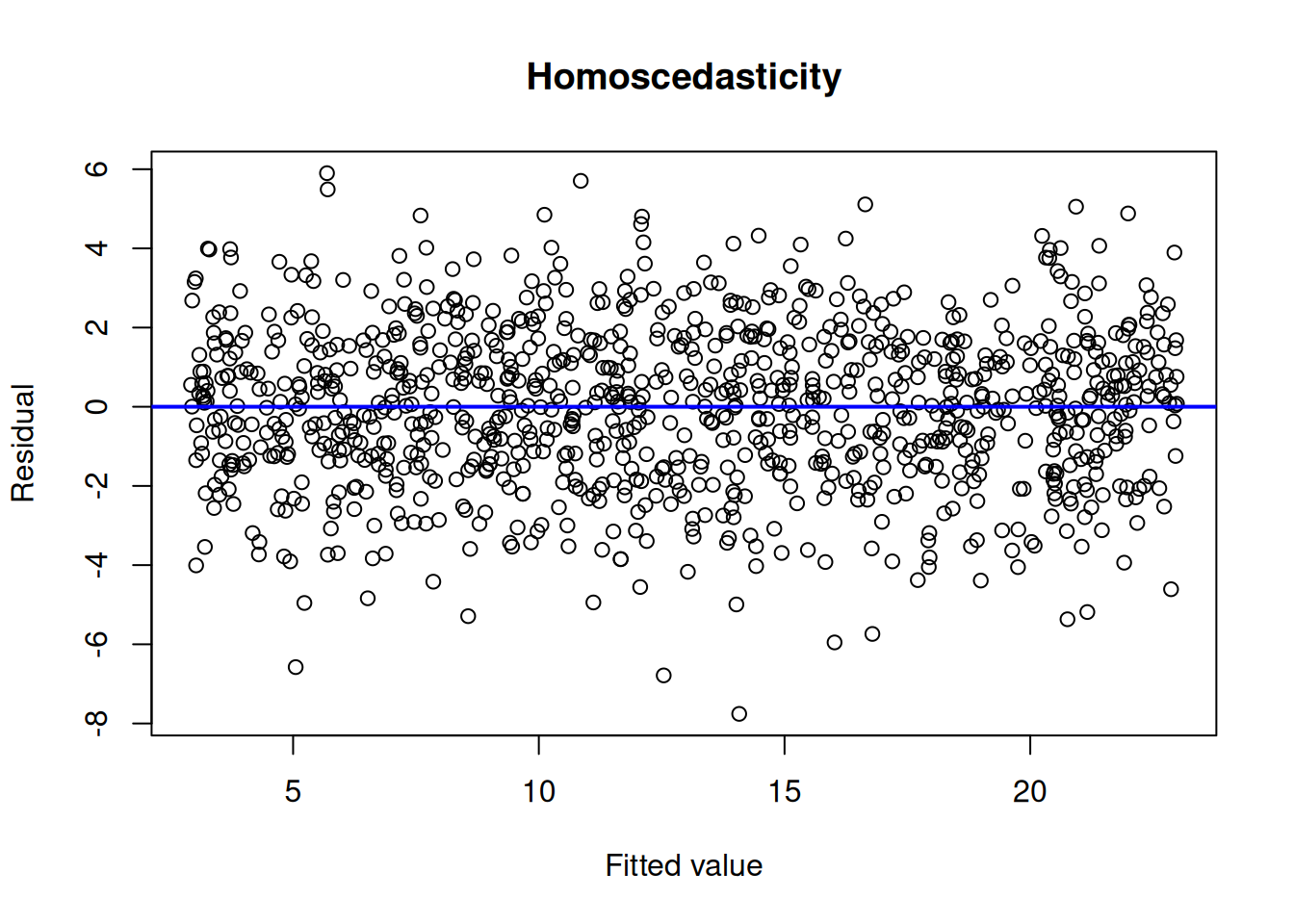
Homoscedasticity of the residuals means that the variance of the residuals does not differ as a function of the outcome variable or as a function of the predictor variable (i.e., the residuals show constant variance as a function of outcome/predictors). If the residuals differ as a function of the outcome or predictor variable, this is called heteroscedasticity.
Those are some of the key assumptions of multiple regression. However, there are additional assumptions of multiple regression, including ones discussed in the chapter on Causal Inference. For instance, the variables included should reflect a causal process such that the predictor variables influence the outcome variable, and not the other way around. That is, the outcome variable should not influence the predictor variables (i.e., there should be no reverse causation). In addition, it is important control for any confound(s). If a confound is not controlled for, this is called omitted-variable bias, and it leads the researcher to incorrectly attribute the effects of the omitted variable to the included variables.
11.5.1 Evaluating and Addressing Assumptions of Multiple Regression
11.5.1.1 Linear Association
To evaluate the shape of the association between the predictor variables and the outcome variable, we can examine scatterplots (Figure 11.2), residual plots (Figure 11.21), marginal model plots (Figure 11.12), added-variable plots (Figure 11.13), and component-plus-residual plots (Figure 11.14). Residual plots depict the residuals (errors) on the y-axis as a function of the fitted values or a specific predictor on the x-axis. Marginal model plots are basically glorified scatterplots that depict the outcome variable (both in terms of observed values and model-fitted values) on the y-axis and the predictor variables on the x-axis. Added-variable plots depict the unique association of each predictor variables with the outcome variable when controlling for all the other predictor variables in the model. Component-plus-residual plots depict partial residuals on the y-axis as a function of each predictor variable on the x-axis, where a partial residual for a given predictor is the effect of a given predictor (thus controlling for all the other predictor variables in the model) plus the residual from the full model.
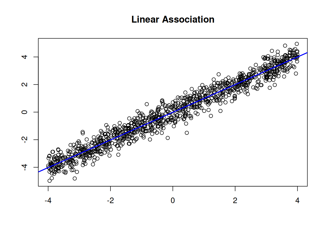
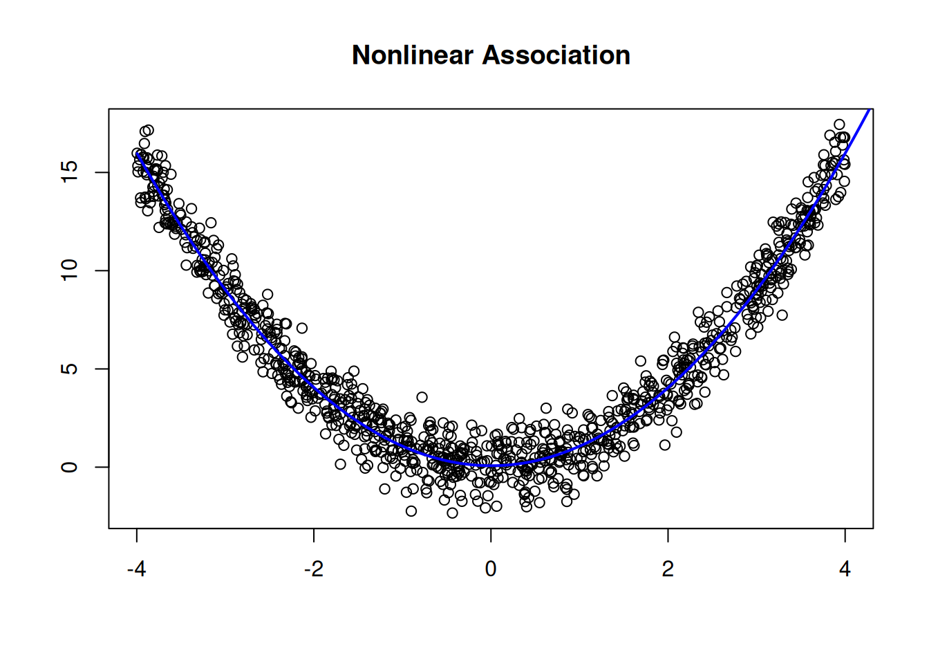
Examples of linear and nonlinear associations are depicted with scatterplots in Figure 11.2.
Figure 11.2: Example Associations Depicted With Scatterplots.
If the shape of the association is nonlinear (as indicated by any of these plots), various approaches may be necessary such as including nonlinear terms (e.g., polynomial terms such as quadratic, cubic, quartic, or higher-degree terms), transforming the predictors (e.g., log, square root, inverse, exponential, Box-Cox, Yeo-Johnson transform), use of splines/piecewise regression, and generalized additive models.
11.5.1.2 Homoscedasticity
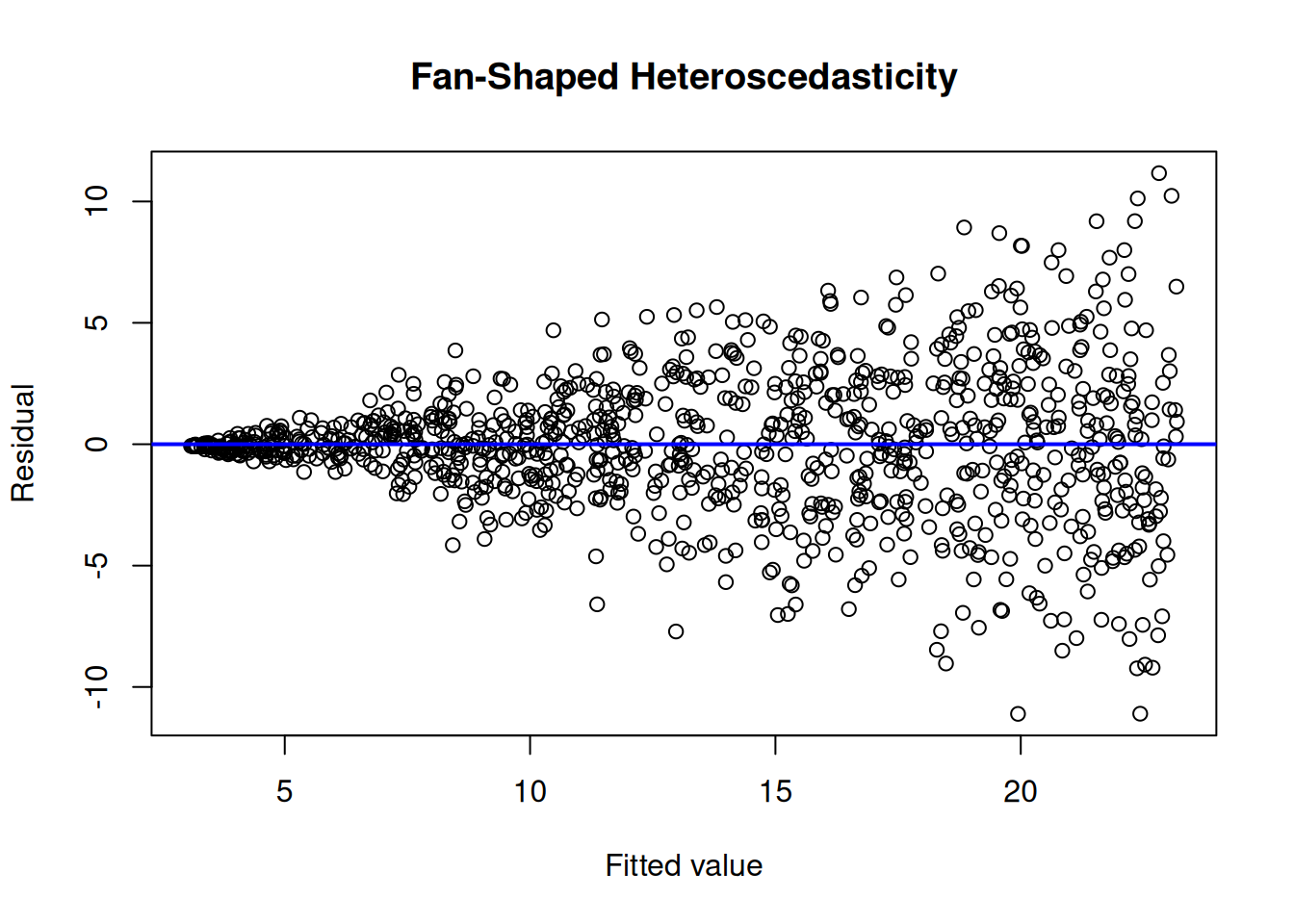
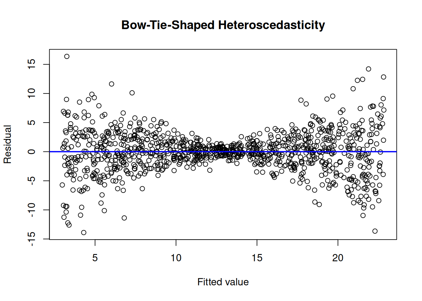
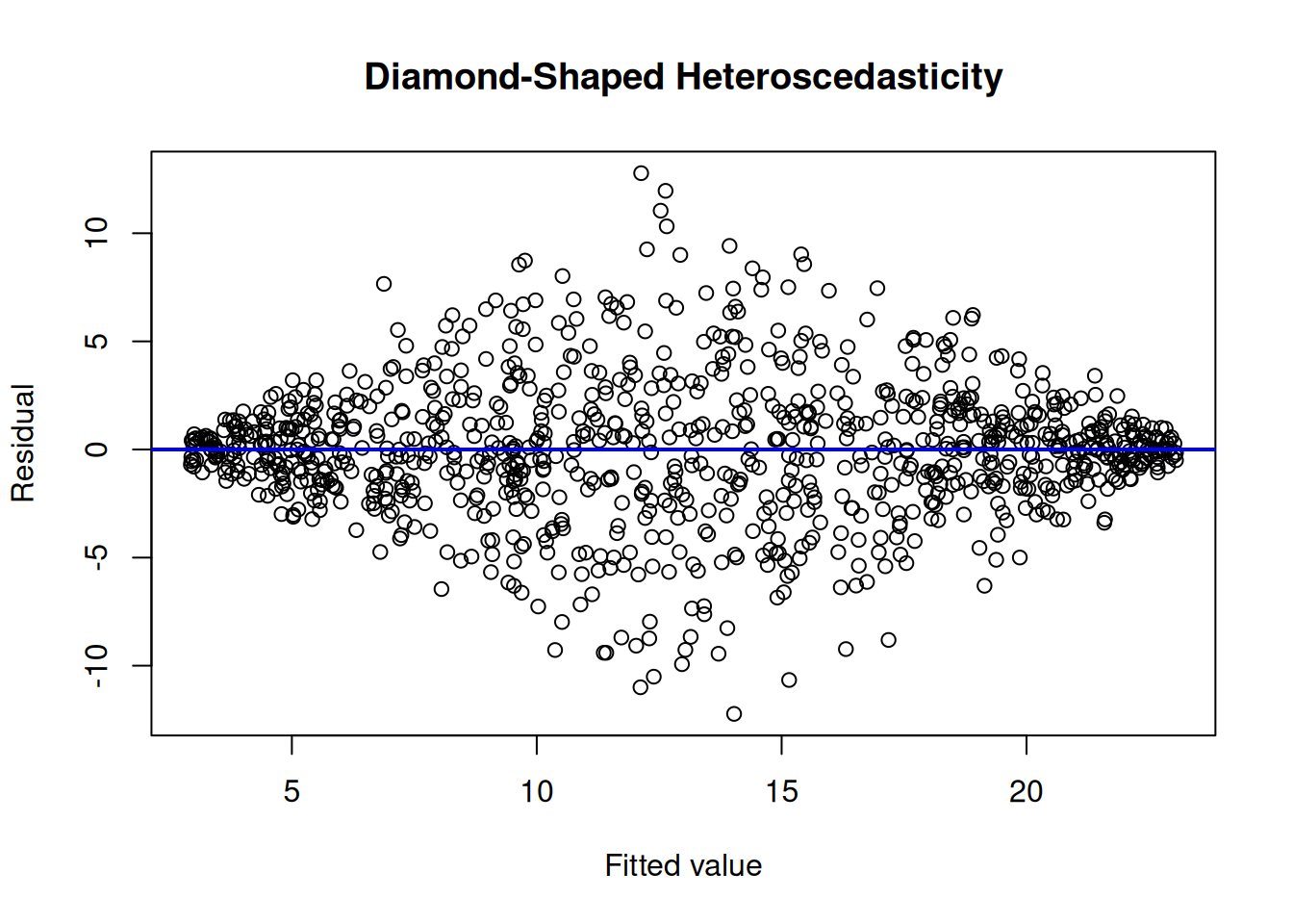
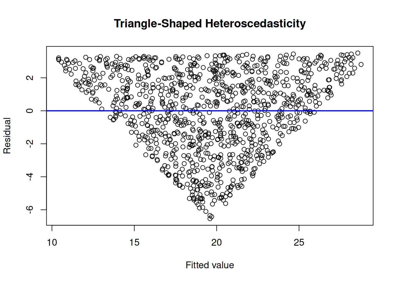
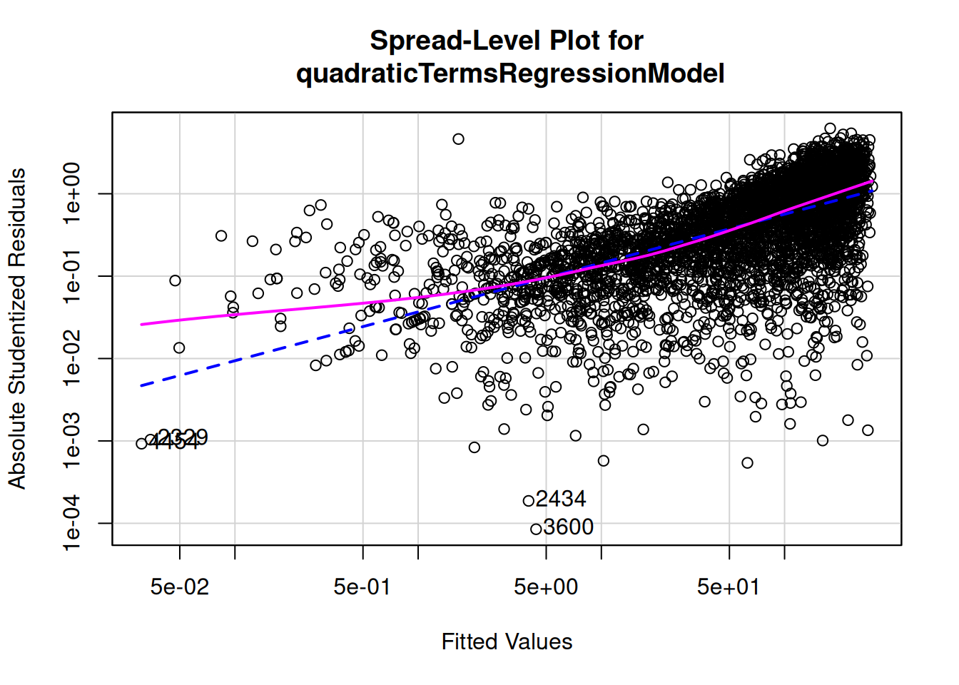
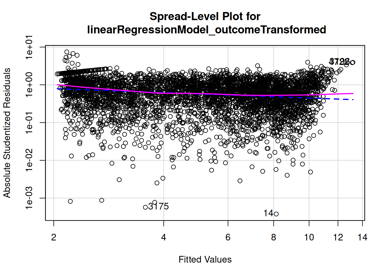
To evaluate homoscedasticity, we can evaluate a residual plot (Figure 11.21) and spread-level plot (Figure 11.22). A residual plot depicts the residuals on the y-axis as a function of the model’s fitted values on the x-axis. Homoscedasticity in a residual plot is identified as a constant spread of residuals versus fitted values—the residuals do not show a fan, cone, or bow-tie shape; a fan, cone, or bow-tie shape indicates heteroscedasticity. In a residual plot, a fan or cone shape indicates increasing or decreasing variance in the residuals as a function of the fitted values; a bow-tie shape indicates that the residuals are smallest in the middle of the fitted values and greatest on the extremes of the fitted values. A spread-level plot depicts the log of the absolute value of studentized residuals on the y-axis as a function of the log of the model’s fitted values on the x-axis. Homoscedasticity in a spread-level plot is identified as a flat slope; a slope that differs from zero indicates heteroscedasticity.
Figure 11.3: Example of Homoscedasticity and Heteroscedasticity in Residual Plots.
If there is heteroscedasticity, it may be necessary to transform the outcome variable to be more normally distributed. The spread-level plot provides a suggested power transformation to transform the outcome variable so that the spread of residuals becomes more uniform across the fitted values.
11.5.1.3 Uncorrelated Residuals
To determine if residuals are correlated by a grouping level, we can examine the proportion of variance that is attributable to the grouping level using the intraclass correlation coefficient (ICC) from a mixed model. The greater the ICC value, the more variance is accounted for by the grouping level, and the more the residuals are intercorrelated. If the residuals are intercorrelated, it may be necessary to account for the grouping structure of the data using a mixed model.
11.5.1.4 Normally Distributed Residuals
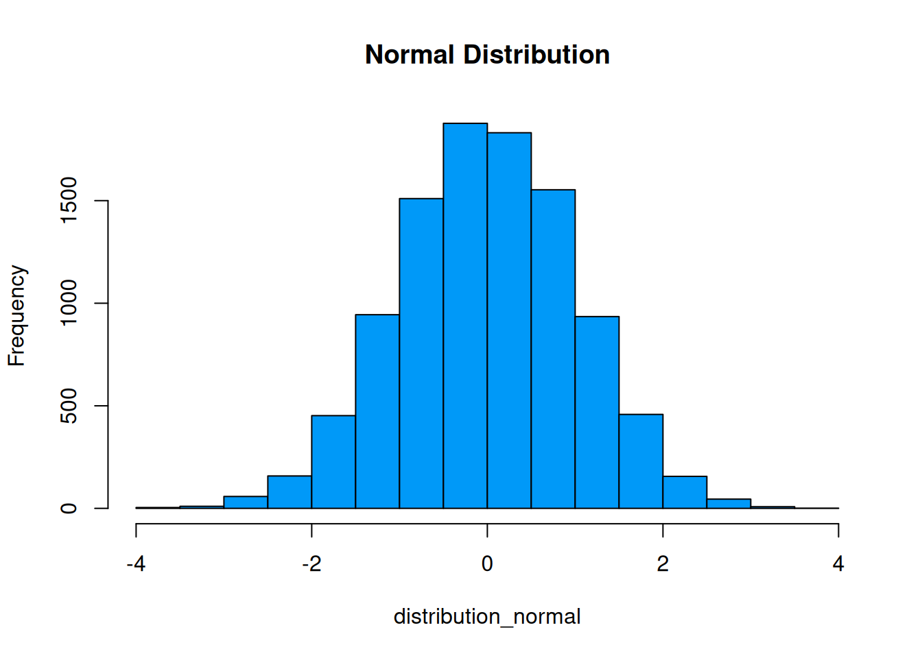
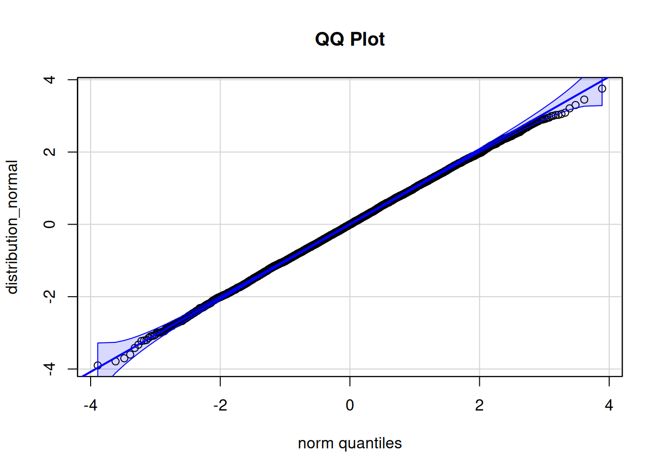
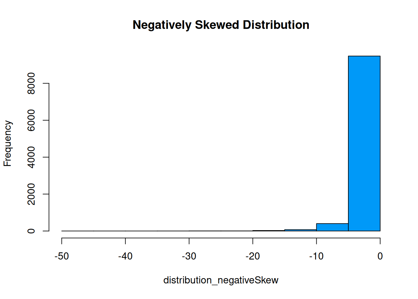
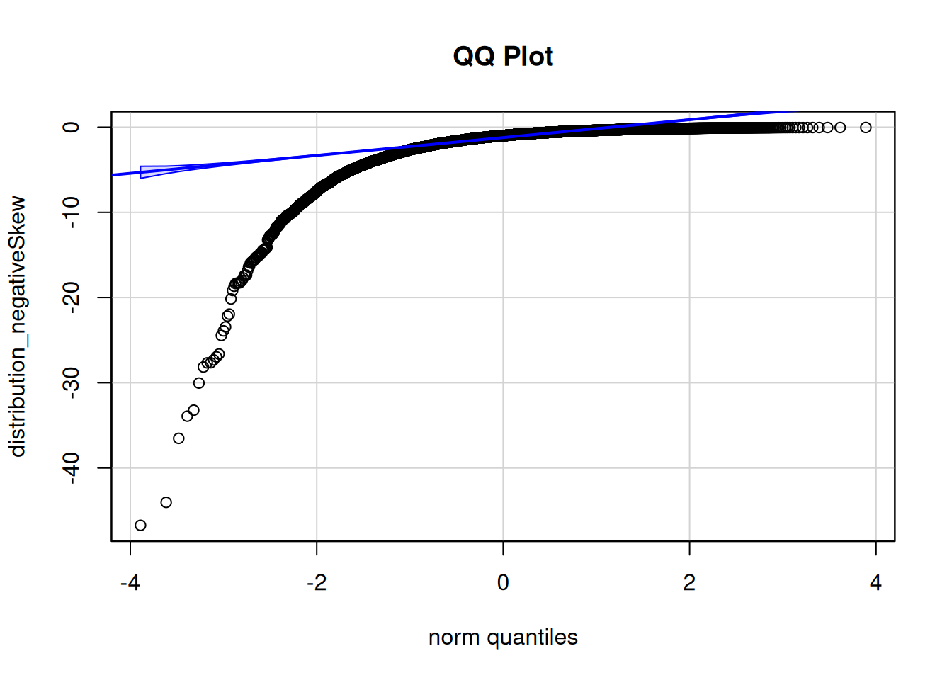
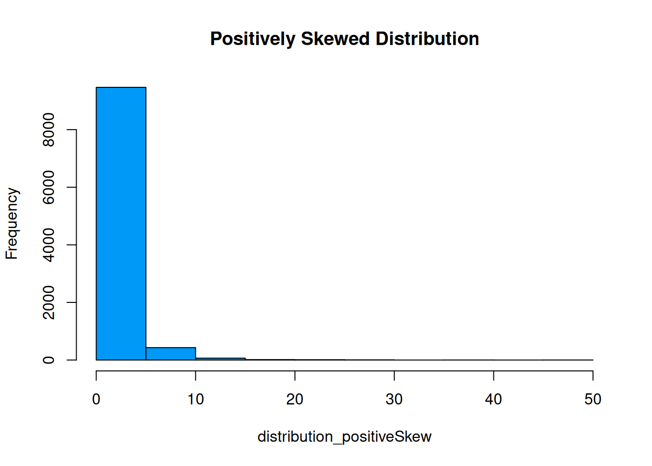
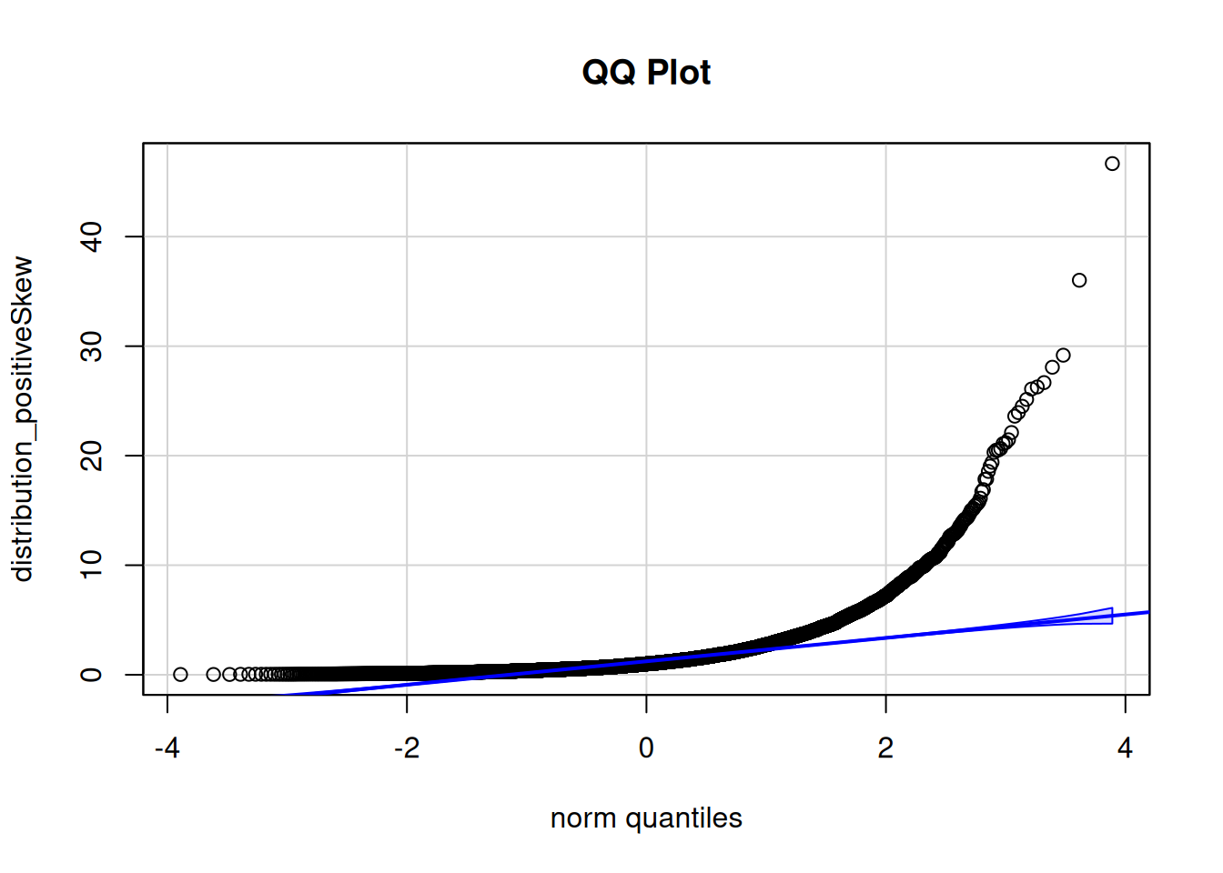
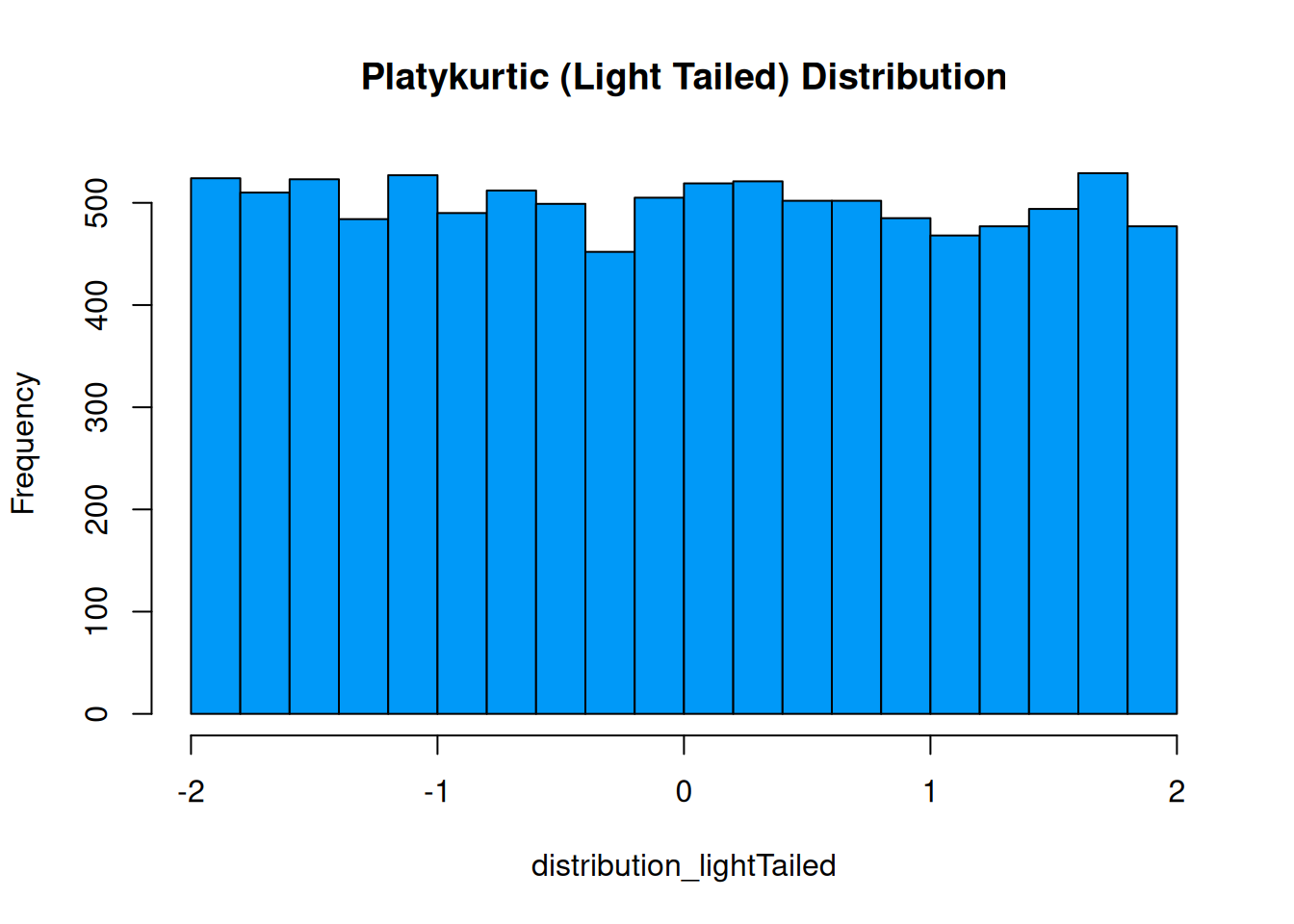
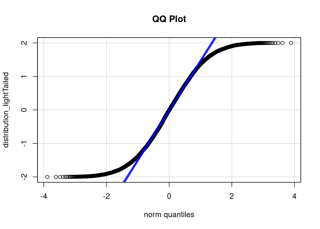
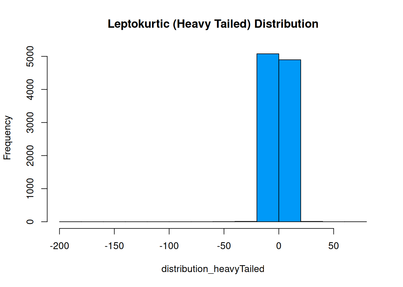
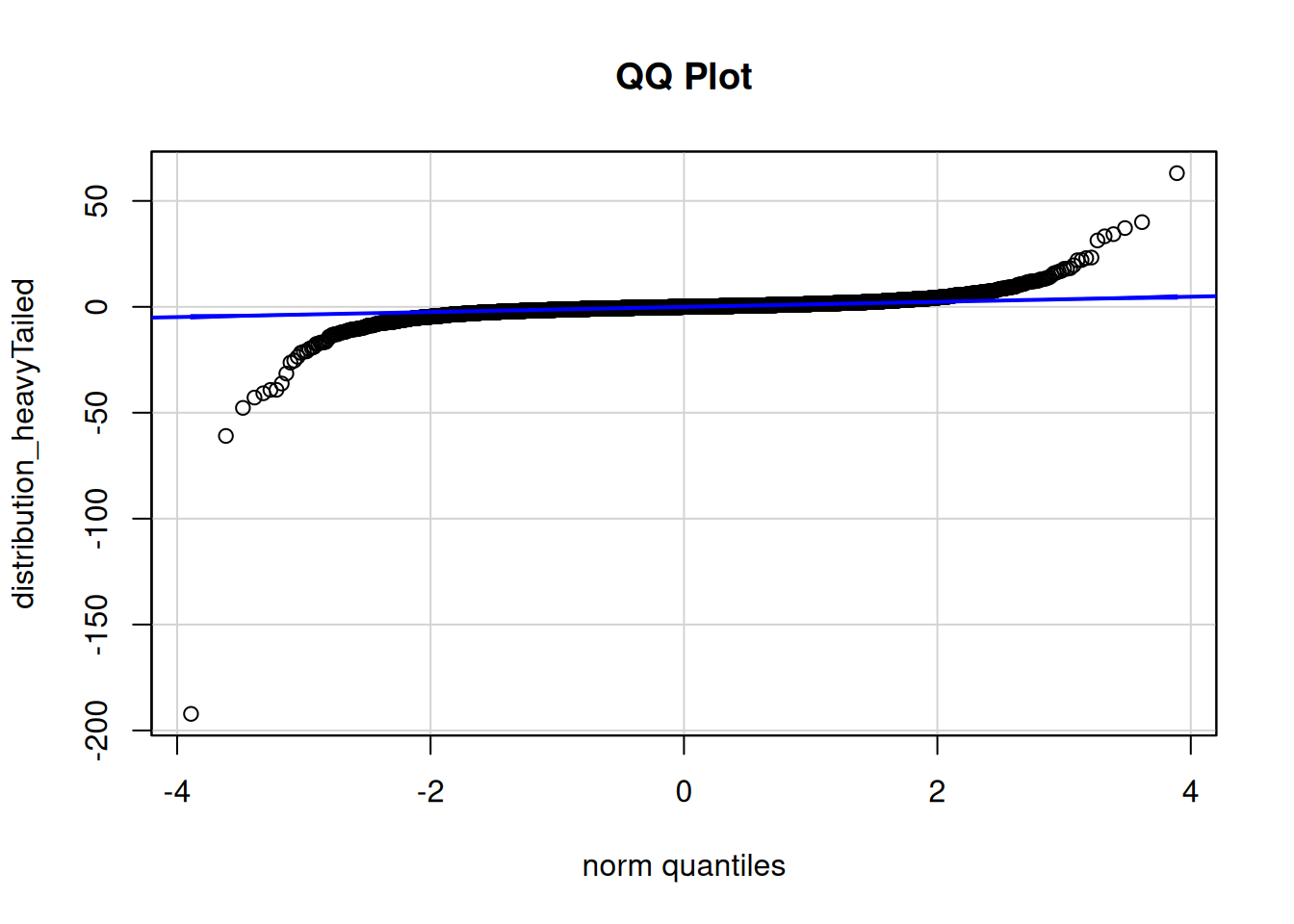
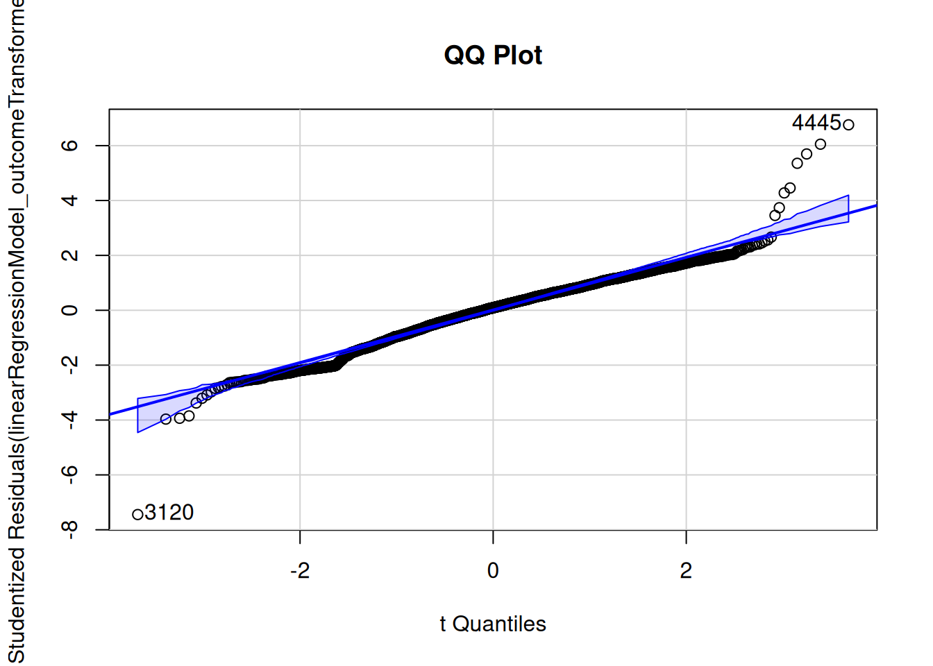
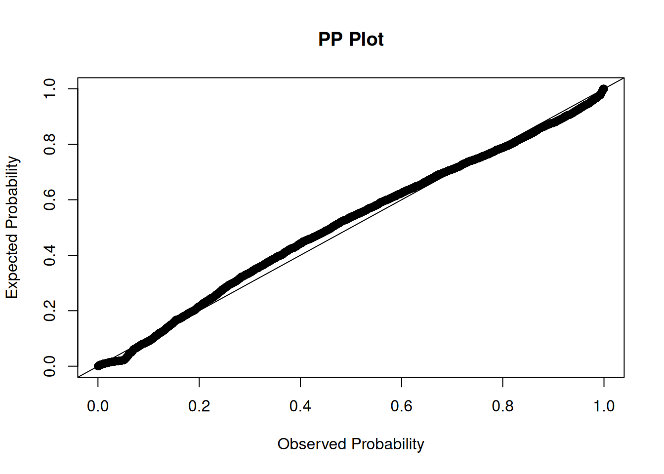
To examine whether residuals are normally distributed, we can examine quantile–quantile (QQ) plots and probability–probability (PP) plots. QQ plots depict quantiles of a sample distribution (y-axis) compared to the quantiles of a theoretical (in this case, normal) distribution (x-axis). PP plots depict cumulative probabilities of a sample distribution (y-axis) compared to those of a theoretical (in this case, normal) distribution (x-axis). QQ plots are particularly useful for identifying deviations from normality in the tails of the distribution; PP plots are particularly useful for identifying deviations from normality in the center of the distribution. Researchers tend to be more concerned about the tails of the distribution, because extreme values tend to have a greater impact on inferences, so researchers tend to use QQ plots more often than PP plots.
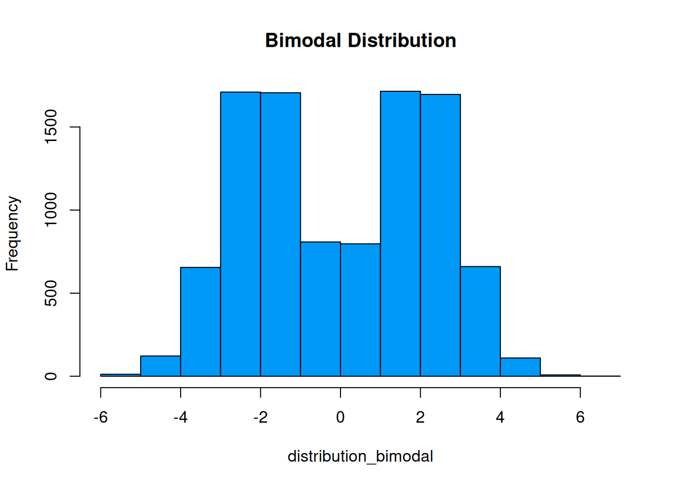
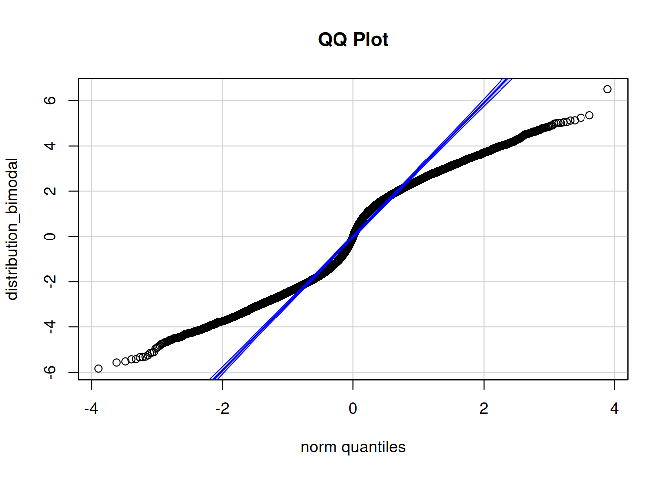
Various examples of QQ plots and deviations from normality are depicted in Figure 11.4.
Figure 11.4: Quantile–Quantile (QQ) Plots of Various Distributions (Right Side) with the Histogram of the Associated Distribution (Left Side).
If the residuals are normally distributed, they will stay close to the diagonal reference line of the QQ and PP plots.
If the residuals are not normally distributed (i.e., they do not stay close to the diagonal reference line of the QQ and PP plots), it may be necessary to transform the outcome variable to be more normally distributed or to use a generalized linear model (GLM) that more closely matches the distribution of the outcome variable (e.g., Poisson, binomial, gamma).
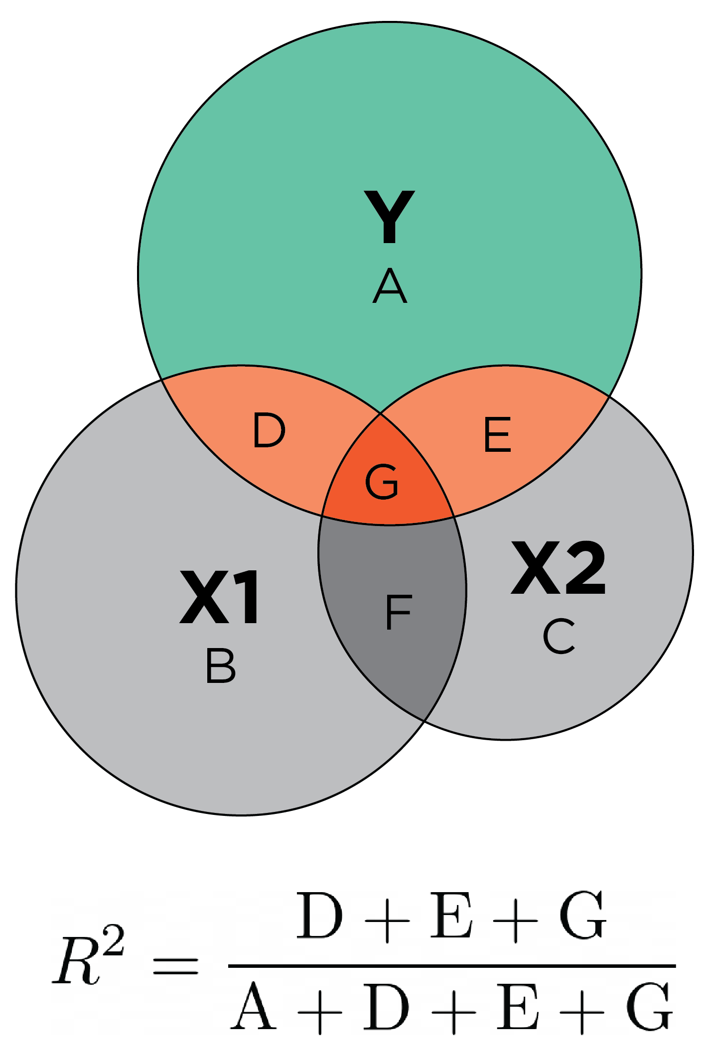
As noted in Section 9.6.6, The coefficient of determination (\(R^2\)) reflects the proportion of variance in the outcome (dependent) variable that is explained by the model predictions (i.e., by the optimal linear combination of the predictor variable(s)), as in Equation 9.31: \(R^2 = \frac{\text{variance explained in }Y}{\text{total variance in }Y}\). Various formulas for \(R^2\) are in Equation 9.19. Larger \(R^2\) values indicate greater accuracy. Multiple regression can be conceptualized with overlapping circles (similar to a venn diagram), where the non-overlapping portions of the circles reflect nonshared variance and the overlapping portions of the circles reflect shared variance, as in Figure 11.29.
Figure 11.5: Conceptual Depiction of Proportion of Variance Explained (\(R^2\)) in an Outcome Variable (\(Y\)) by Multiple Predictors (\(X1\) and \(X2\)) in Multiple Regression. The size of each circle represents the variable’s variance. The proportion of variance in \(Y\) that is explained by the predictors is depicted by the areas in orange. The dark orange space (\(G\)) is where multiple predictors explain overlapping variance in the outcome. Overlapping variance that is explained in the outcome (\(G\)) will not be recovered in the regression coefficients when both predictors are included in the regression model. From Petersen (2024) and Petersen (2025).
One issue with \(R^2\) is that it increases as the number of predictors increases, which can lead to overfitting if using \(R^2\) as an index to compare models for purposes of selecting the “best-fitting” model. Consider the following example (adapted from Petersen (2025)) in which you have one predictor variable and one outcome variable, as shown in Table 11.1.
Table 11.1: Example Data of Predictor (x1) and Outcome (y) Used for Regression Model.
y
x1
7
1
13
2
29
7
10
2
Using the data, the best fitting regression model is: \(y =\) 3.98 \(+\) 3.59 \(\cdot x_1\). In this example, the \(R^2\) is 0.98. The equation is not a perfect prediction, but with a single predictor variable, it captures the majority of the variance in the outcome.
Now consider the following example where you add a second predictor variable to the data above, as shown in Table 11.2.
Table 11.2: Example Data of Predictors (x1 and x2) and Outcome (y) Used for Regression Model.
y
x1
x2
7
1
3
13
2
5
29
7
1
10
2
2
With the second predictor variable, the best fitting regression model is: \(y =\) 0.00 + 4.00 \(\cdot x_1 +\) 1.00 \(\cdot x_2\). In this example, the \(R^2\) is 1.00. The equation with the second predictor variable provides a perfect prediction of the outcome.
Providing perfect prediction with the right set of predictor variables is the dream of multiple regression. So, using multiple regression, we often add predictor variables to incrementally improve prediction. Knowing how much variance would be accounted for by random chance follows Equation 11.7:
\[
E(R^2) = \frac{K}{n-1}
\tag{11.7}\]
where \(E(R^2)\) is the expected value of \(R^2\) (the proportion of variance explained), \(K\) is the number of predictor variables, and \(n\) is the sample size. The formula demonstrates that the more predictor variables in the regression model, the more variance will be accounted for by chance. With many predictor variables and a small sample, you can account for a large share of the variance merely by chance.
As an example, consider that we have 13 predictor variables to predict fantasy performance for 43 players. Assume that, with 13 predictor variables, we explain 38% of the variance (\(R^2 = .38; r = .62\)). We explained a lot of the variance in the outcome, but it is important to consider how much variance could have been explained by random chance: \(E(R^2) = \frac{K}{n-1} = \frac{13}{43 - 1} = .31\). We expect to explain 31% of the variance, by chance, in the outcome. So, 82% of the variance explained was likely spurious (i.e., \(\frac{.31}{.38} = .82\)). As the sample size increases, the spuriousness decreases. To account for the number of predictor variables in the model, we can use a modified version of \(R^2\) called adjusted \(R^2\) (\(R^2_{adj}\)), described next.
11.6.2 Adjusted \(R^2\) (\(R^2_{adj}\))
Adjusted \(R^2\) (\(R^2_{adj}\)) accounts for the number of predictor variables in the model, based on how much would be expected to be accounted for by chance to penalize overfitting. Adjusted \(R^2\) (\(R^2_{adj}\)) reflects the proportion of variance in the outcome (dependent) variable that is explained by the model predictions over and above what would be expected to be accounted for by chance, given the number of predictor variables in the model. The formula for adjusted \(R^2\) (\(R^2_{adj}\)) is in Equation 11.8:
where \(p\) is the number of predictor variables in the model, and \(n\) is the sample size.
11.7 How Much Variance Each Predictor Explains
Another estimate of effect size in addition to standardized regression coefficients is the squared semi-partial correlation (\(sr^2\)). The squared semi-partial correlation reflects the proportion of variance in the outcome variable that is uniquely explained by each predictor variable. The total model \(R^2\) minus the sum of all the squared semi-partial correlations reflects the proportion of variance in the outcome variable that is explained by the common variance among the predictor variables.
11.8 Overfitting
Statistical models applied to big data (e.g., data with many predictor variables) can overfit the data, which means that the statistical model accounts for error variance, which will not generalize to future samples. So, even though an overfitting statistical model appears to be accurate because it is accounting for more variance, it is not actually that accurate—it will predict new data less accurately than how accurately it accounts for the data with which the model was built. Overfitting is most likely to occur when the model is too complex relative to the sample size (e.g., many predictor variables or parameters) In the case of fantasy football analytics, this is especially relevant because there are hundreds if not thousands of variables we could consider for inclusion and many, many players when considering historical data.
Consider an example where you develop an algorithm to predict players’ fantasy performance based on 2024 data using hundreds of predictor variables. To some extent, these predictor variables will likely account for true variance (i.e., signal) and error variance (i.e., noise). If we were to apply the same algorithm based on the 2025 prediction model to 2026 data, the prediction model would likely predict less accurately than with 2025 data. The regression coefficients (and resulting accuracy) tend to become weaker when applied to new data, a phenomenon called shrinkage, which is described in Section 15.7.1. For instance, shrinkage is observed when applying multiple regression models to new data in Section 19.7 and when applying machine learning models to new data in Section 19.8.
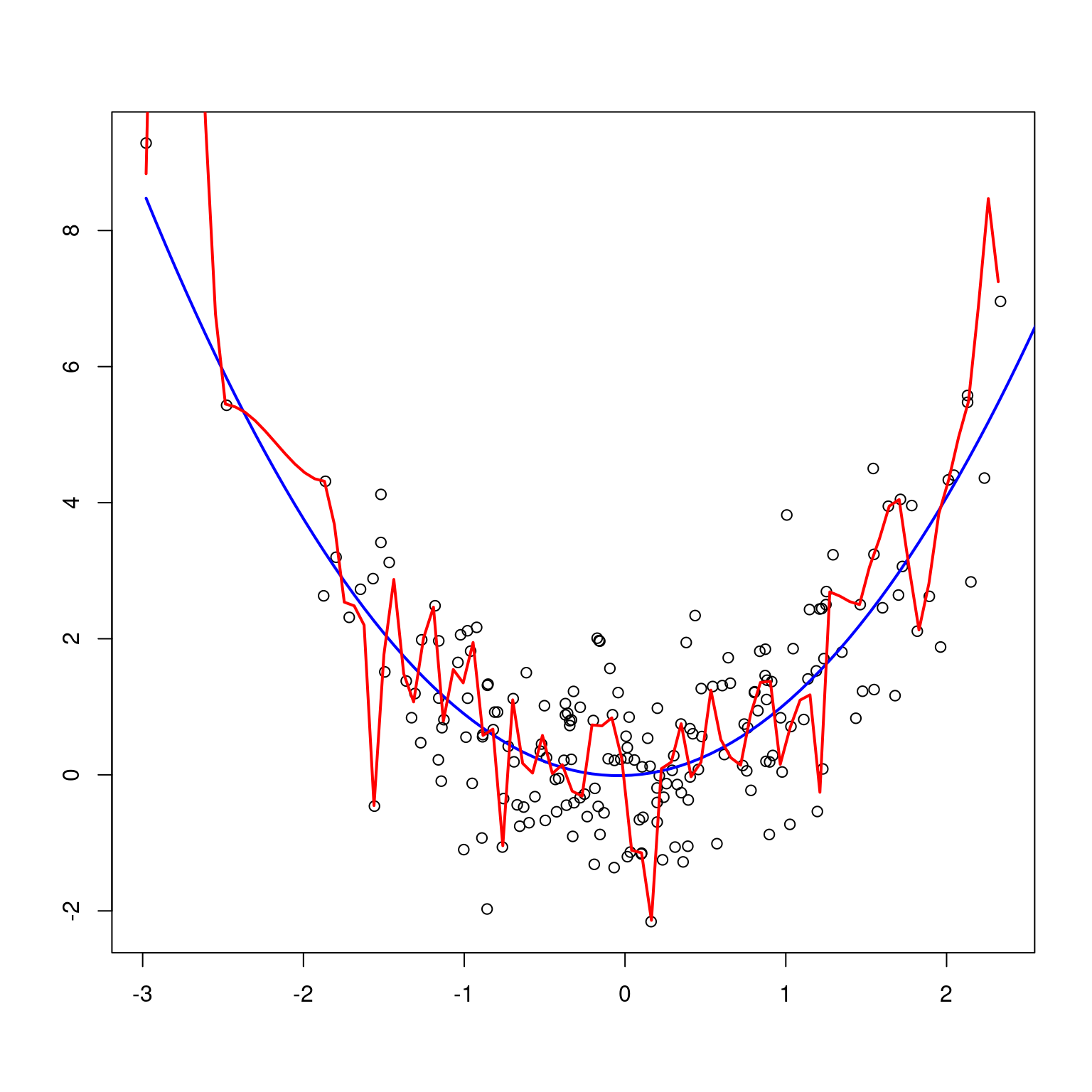
In Figure 11.6, the blue line represents the true distribution of the data, and the red line is an overfitting model:
Figure 11.6: Over-fitting Model in Red Relative to the True Distribution of the Data in Blue. From Petersen (2024) and Petersen (2025).
11.9 Covariates
Covariates are variables that you include in the statistical model to try to control for them so you can better isolate the unique contribution of the predictor variable(s) in relation to the outcome variable. Use of covariates examines the association between the predictor variable and the outcome variable when holding people’s level constant on the covariates. Inclusion of confounds as covariates allows potentially gaining a more accurate estimate of the causal effect of the predictor variable on the outcome variable. Ideally, you want to include any and all confounds as covariates. As described in Section 8.5.2.1, confounds are third variables that influence both the predictor variable and the outcome variable and explain their association. Covariates are potentially (but not necessarily) confounds. For instance, you might include the player’s age as a covariate in a model that examines whether a player’s 40-yard dash time at the NFL Combine predicts their fantasy points in their rookie year, but it may not be a confound.
However, it is worth noting that, for several reasons, including a variable as a covariate in a model does not necessarily fully control for that construct. First, your measure of the covariate has measurement error and may not fully capture the construct, which can lead to residual confounding. Second, including the covariate only accounts for the linear effect of that variable. The variable (e.g., age) could have nonlinear effects that are not captured by the linear term (and may require nonlinear terms, e.g., quadratic). Third, the construct could interact with other constructs, which would also not be captured by the linear term (and may require interaction terms). Thus, it is important to consider the reliability of the covariate, and the ways in which the covariate is related to the outcome including any nonlinearity and interactions.
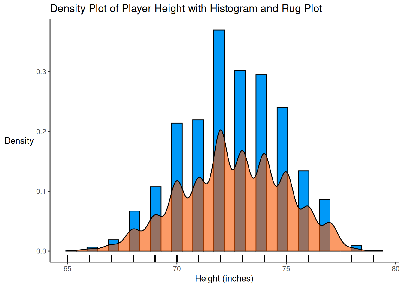
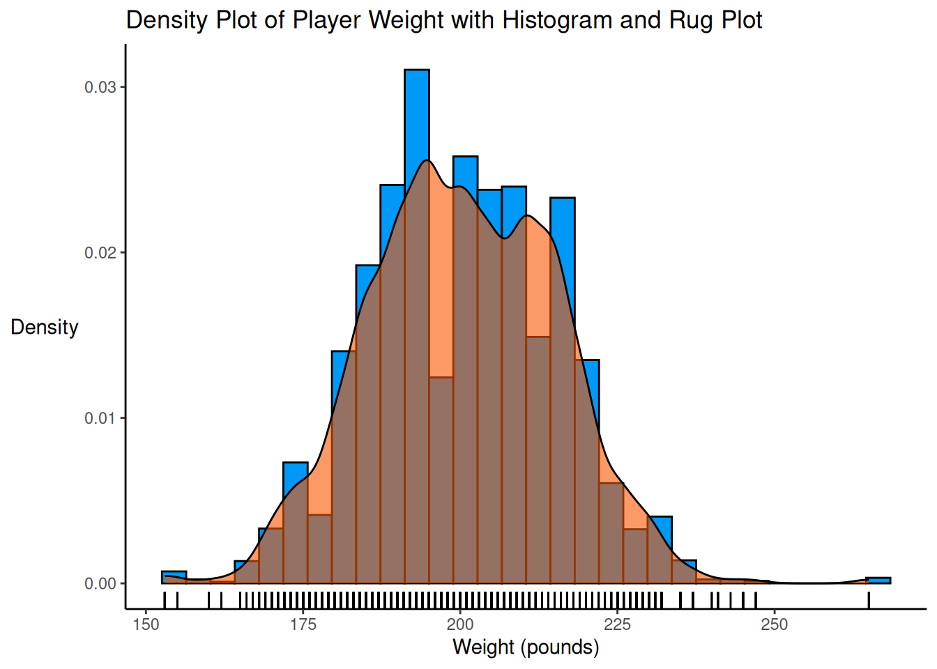
11.10 Example: Predicting Wide Receivers’ Fantasy Points
Let’s say we want to use a number of variables to predict a wide receiver’s fantasy performance. We want to consider several predictors, including the player’s age, height, weight, and target share. Target share is computed as the number of targets a player receives divided by the team’s total number of targets. We have only a few predictors and our sample size is large enough such that overfitting is not likely a concern.
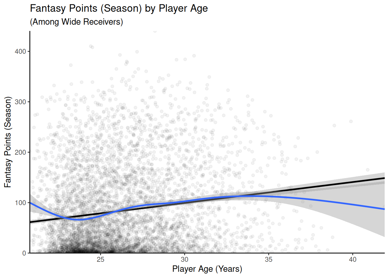
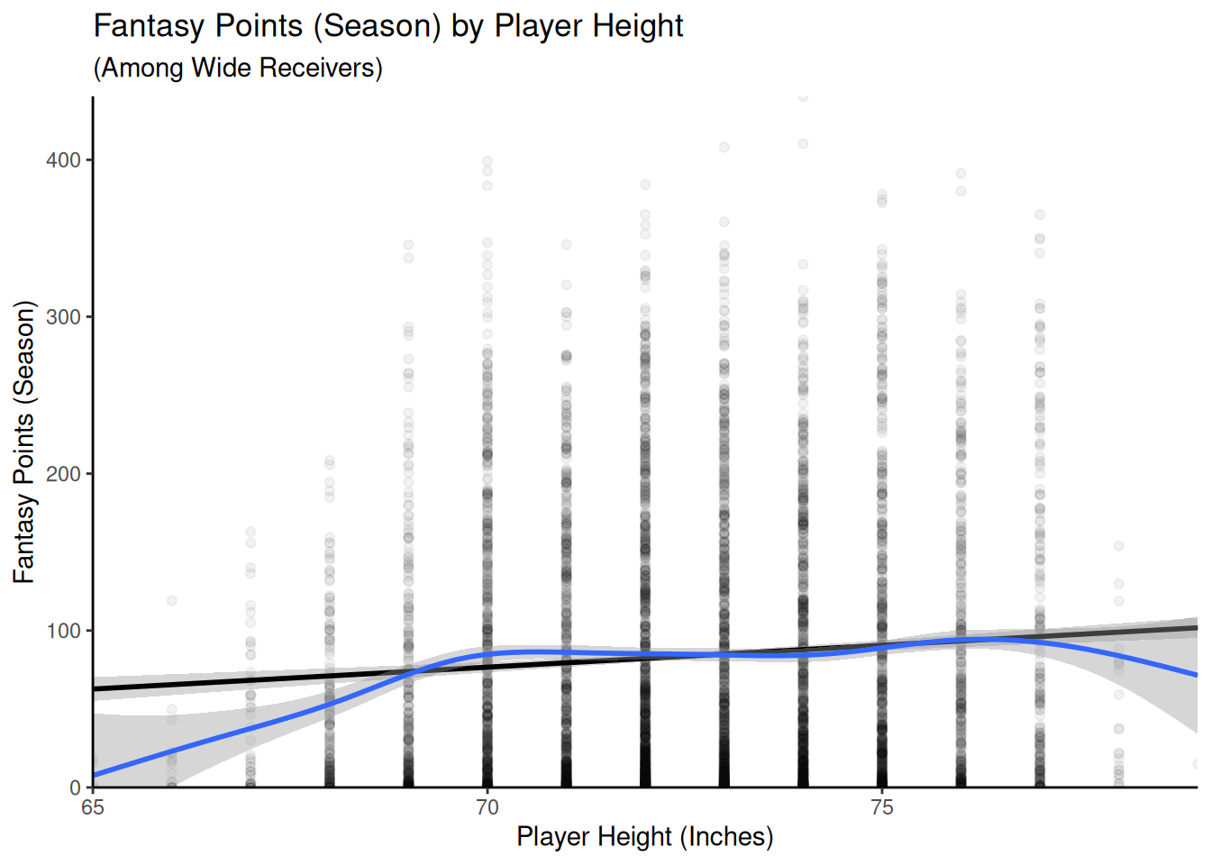
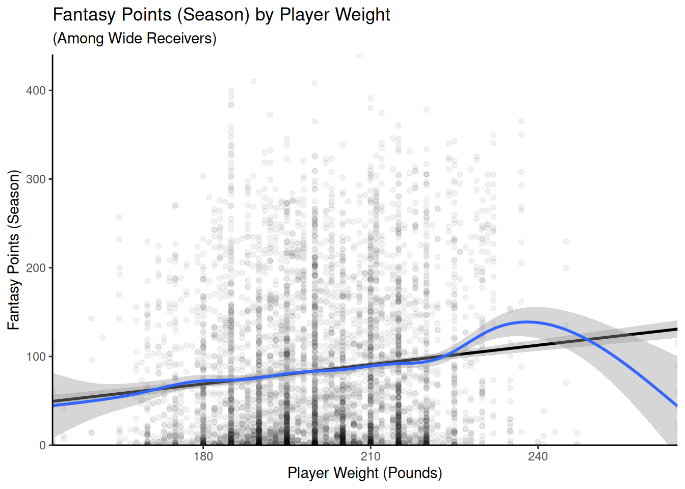
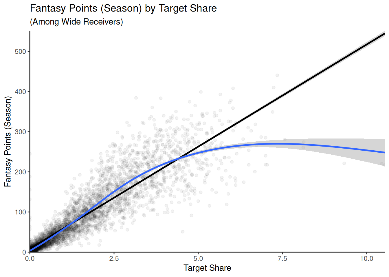
Figure 11.8: Scatterplots With Fantasy Points (Season) Among Wide Receivers. The linear best-fit line is in black. The nonlinear best-fit line is in blue.
There are some suggestions of potential nonlinearity, such as an inverted-U-shaped association between height and fantasy points, suggesting that there may an optimal range for height among Wide Receivers—being too short or too tall could be a disadvantage. In addition, target share shows a weakening association as target share increases. Thus, after evaluating the linear association between the predictors and outcome, we will also examine the possibility for curvilinear associations.
11.10.3 Estimate Multiple Regression Model
Now that we have examined descriptive statistics and bivariate associations, let’s first estimate a multiple regression model with only linear terms:
Call:
lm(formula = fantasyPoints ~ age + height + weight + target_share,
    data = player_stats_seasonal %>% filter(position %in% c("WR")),
    na.action = "na.exclude")

Residuals:
    Min      1Q  Median      3Q     Max
-746.79  -18.14  -10.12   10.34  293.12

Coefficients:
              Estimate Std. Error t value Pr(>|t|)
(Intercept)  -27.36726   22.98098  -1.191  0.23377
age            0.63790    0.21398   2.981  0.00289 **
height        -0.13754    0.41579  -0.331  0.74081
weight         0.19270    0.06573   2.932  0.00339 **
target_share 750.28584    7.09218 105.791  < 2e-16 ***
---
Signif. codes:  0 '***' 0.001 '**' 0.01 '*' 0.05 '.' 0.1 ' ' 1

Residual standard error: 44.83 on 4692 degrees of freedom
  (953 observations deleted due to missingness)
Multiple R-squared:  0.7139,    Adjusted R-squared:  0.7136
F-statistic:  2927 on 4 and 4692 DF,  p-value: < 2.2e-16
The only terms that were significantly associated with fantasy performance among Wide Receivers are weight and target share, both of which showed a positive association with fantasy points.
The deltaR-square values: the change in the R-square
      observed when a single term is removed.
Same as the square of the 'semi-partial correlation coefficient'
             deltaRsquare
age          5.419797e-04
height       6.673050e-06
weight       5.241517e-04
target_share 6.824913e-01
$CC
                                                Coefficient     % Total
Unique to age                                        0.0005        0.08
Unique to height                                     0.0000        0.00
Unique to weight                                     0.0005        0.07
Unique to target_share                               0.6825       95.60
Common to age, and height                            0.0000        0.00
Common to age, and weight                            0.0000        0.00
Common to height, and weight                         0.0005        0.06
Common to age, and target_share                      0.0136        1.90
Common to height, and target_share                   0.0003        0.04
Common to weight, and target_share                   0.0091        1.27
Common to age, height, and weight                    0.0000        0.00
Common to age, height, and target_share              0.0001        0.01
Common to age, weight, and target_share              0.0006        0.09
Common to height, weight, and target_share           0.0064        0.89
Common to age, height, weight, and target_share     -0.0002       -0.03
Total                                                0.7139      100.00

$CCTotalbyVar
             Unique Common  Total
age          0.0005 0.0141 0.0146
height       0.0000 0.0070 0.0070
weight       0.0005 0.0164 0.0169
target_share 0.6825 0.0298 0.7123
$DA
                               k          R2      age.Inc   height.Inc
age                            1 0.014629177           NA 7.127246e-03
height                         1 0.007012135 0.0147442880           NA
weight                         1 0.016896454 0.0142030198 3.839378e-04
target_share                   1 0.712336807 0.0005451049 4.512355e-04
age,height                     2 0.021756423           NA           NA
age,weight                     2 0.031099474           NA 2.809777e-04
height,weight                  2 0.017280392 0.0141000597           NA
age,target_share               2 0.712881912           NA 4.656973e-04
height,target_share            2 0.712788042 0.0005595667           NA
weight,target_share            2 0.713320242 0.0005448459 9.539226e-06
age,height,weight              3 0.031380451           NA           NA
age,height,target_share        3 0.713347609           NA           NA
age,weight,target_share        3 0.713865088           NA 6.673050e-06
height,weight,target_share     3 0.713329781 0.0005419797           NA
age,height,weight,target_share 4 0.713871761           NA           NA
                                 weight.Inc target_share.Inc
age                            0.0164702966        0.6982527
height                         0.0102682564        0.7057759
weight                                   NA        0.6964238
target_share                   0.0009834349               NA
age,height                     0.0096240282        0.6915912
age,weight                               NA        0.6827656
height,weight                            NA        0.6960494
age,target_share               0.0009831759               NA
height,target_share            0.0005417386               NA
weight,target_share                      NA               NA
age,height,weight                        NA        0.6824913
age,height,target_share        0.0005241517               NA
age,weight,target_share                  NA               NA
height,weight,target_share               NA               NA
age,height,weight,target_share           NA               NA

$CD
              age       height       weight target_share
CD:0 0.0146291771 7.012135e-03 0.0168964539    0.7123368
CD:1 0.0098308042 2.654140e-03 0.0092406626    0.7001508
CD:2 0.0050681575 2.520714e-04 0.0037163142    0.6901354
CD:3 0.0005419797 6.673050e-06 0.0005241517    0.6824913

$GD
         age       height       weight target_share
 0.007517530  0.002481255  0.007594396  0.696278581
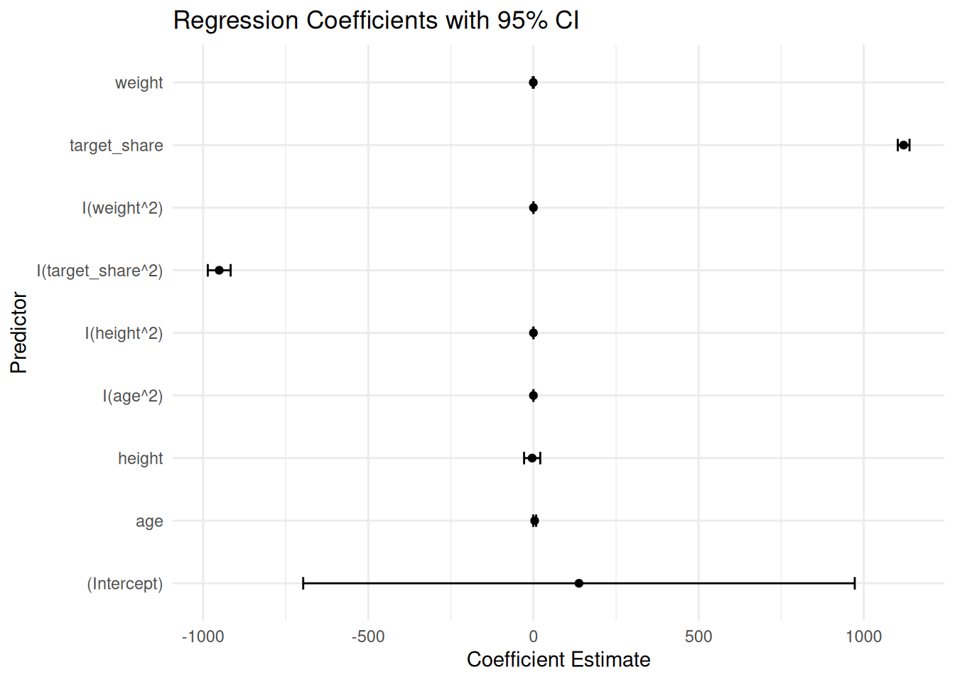
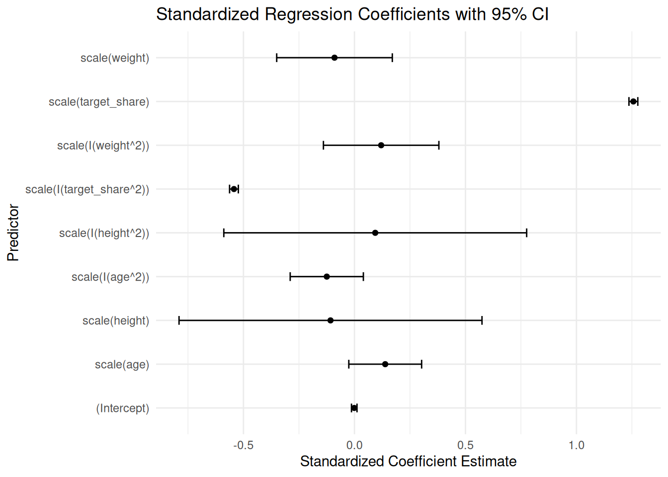
Figure 11.10: Standardized Regression Coefficients with 95% Confidence Interval.
11.10.7.2 Model-Implied Association
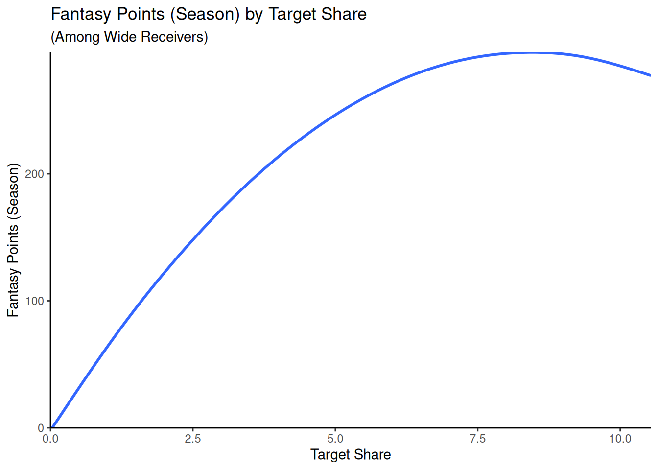
If we wanted to visualize the shape of the model-implied association between target share and fantasy points, we could generate the model-implied predictions using the data range that we want to visualize.
Figure 11.11: Model-Implied Predictions of A Wide Receiver’s Fantasy Points as a Function of Target Share. The model-implied predictions were estimated based on a multiple regression model.
We could also generate the model-implied prediction of fantasy points for any value of the predictor variables. For instance, here are the number of fantasy points expected for a Wide Receiver who is 23 years old, is 6’2” tall (72 inches), weighs 200 pounds, and has a target share of 50% (i.e., 0.5):
there is homoscedasticity of the residuals; the residuals do not differ as a function of the predictor variables or as a function of the outcome variable
the residuals are independent; they are uncorrelated with each other
the residuals are normally distributed
11.10.8.1 Linear Association
We evaluated the shape of the association between the predictor variables and the outcome variables using scatterplots. We accounted for potential curvilinearity in the associations with a quadratic term. Other ways to account for nonlinearity, in addition to polynomials, include transforming predictors, use of splines/piecewise regression, and generalized additive models.
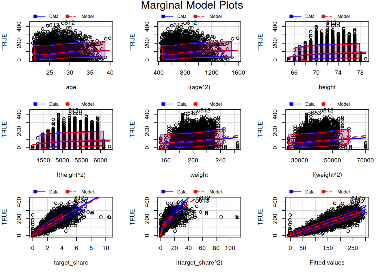
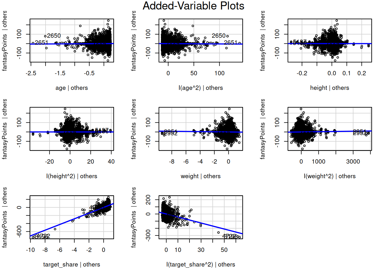
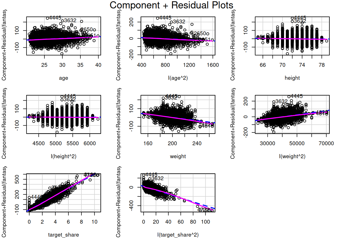
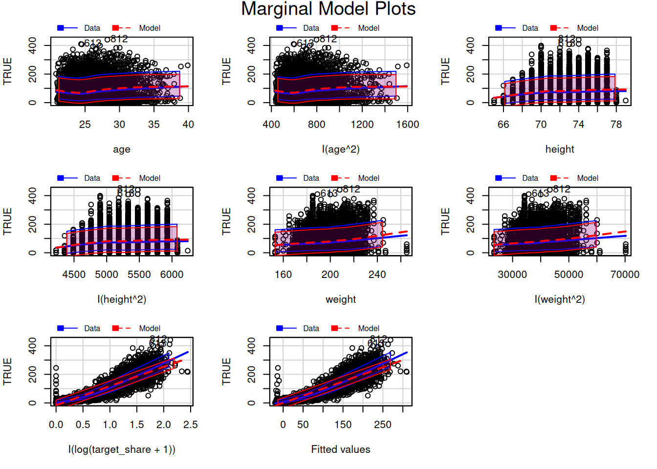
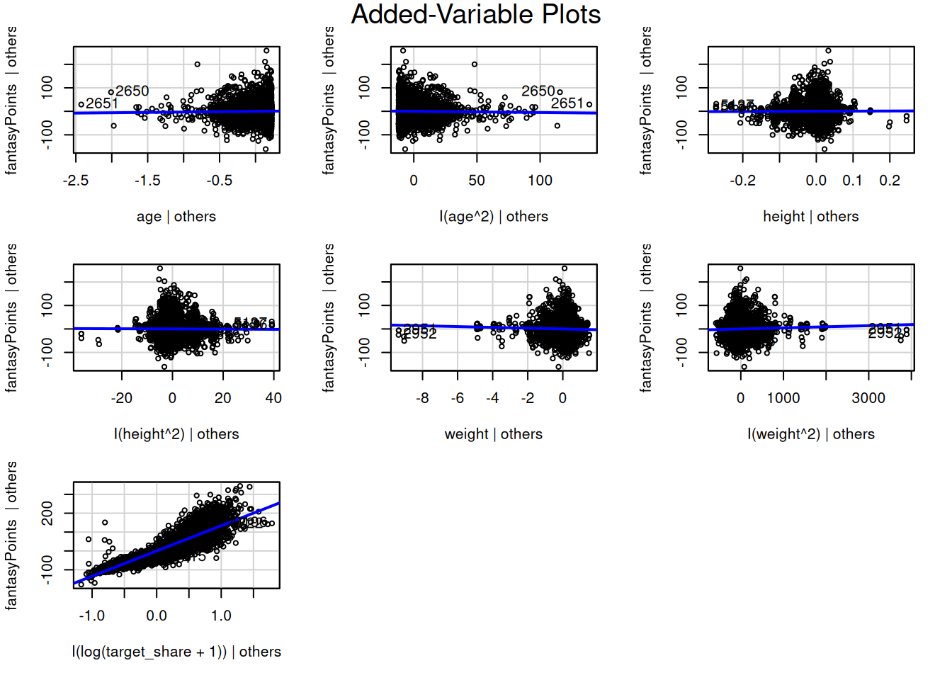
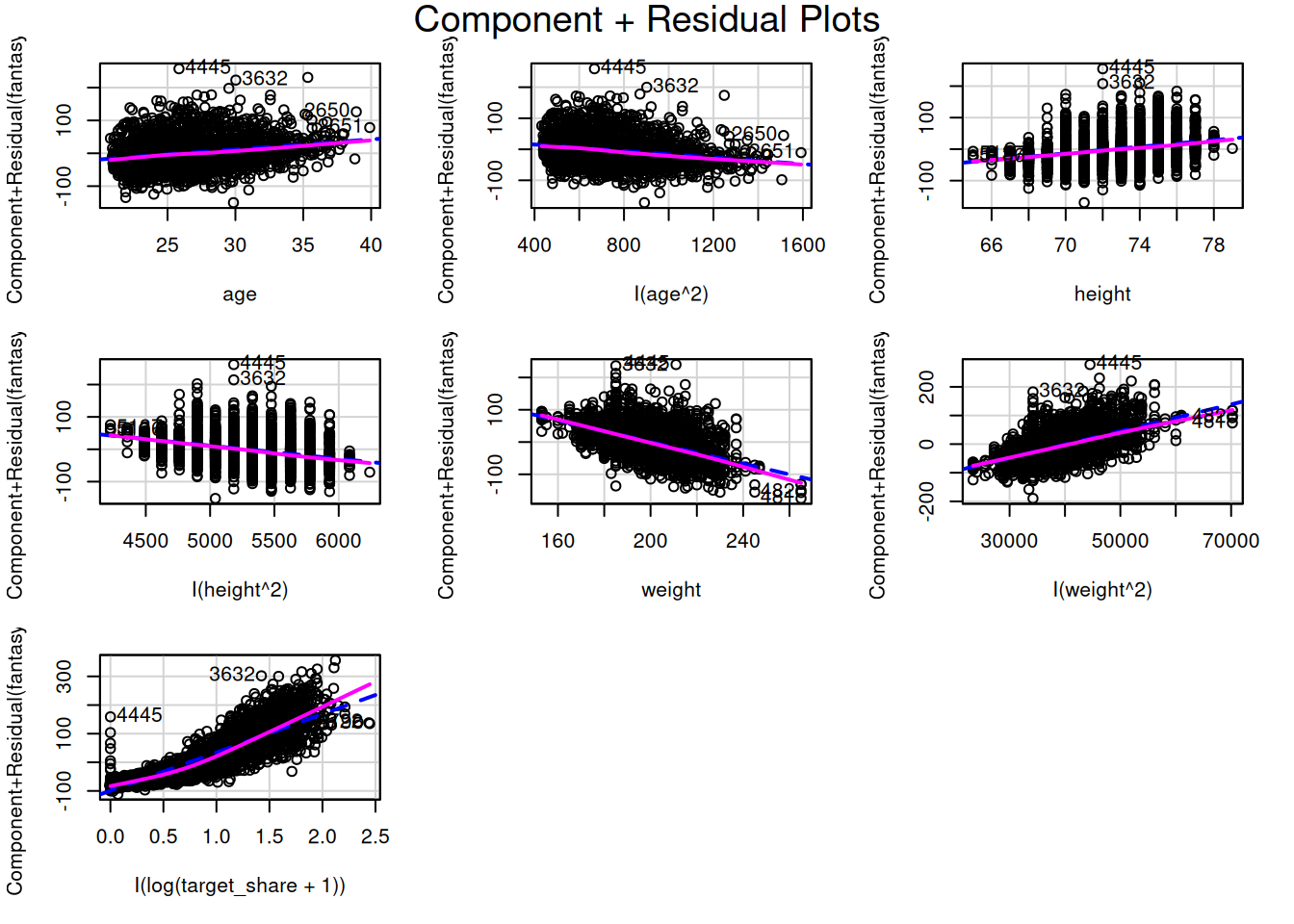
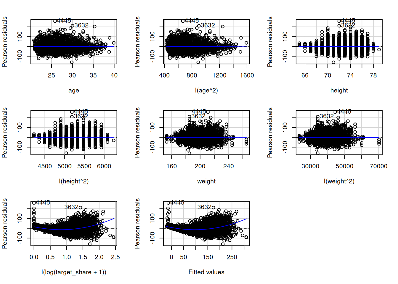
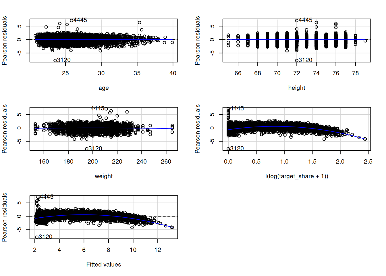
To evaluate for potential nonlinearity in the associations, we can also evaluate residual plots (Figure 11.21), marginal model plots (Figure 11.12), added-variable plots (Figure 11.13), and component-plus-residual plots (Figure 11.14) from the car package (Fox et al., 2024; Fox & Weisberg, 2019). For evaluating linearity, we would expect minimal bend/curvature in the lines.
The marginal model plots (Figure 11.12), residual plots (Figure 11.21), and component-plus-residual plots (Figure 11.14) suggest that the nonlinearity of the association between target share and fantasy points may not be fully captured by the quadratic term. Thus, we may need to apply a different approach to handling the nonlinear association between target share and fantasy points.
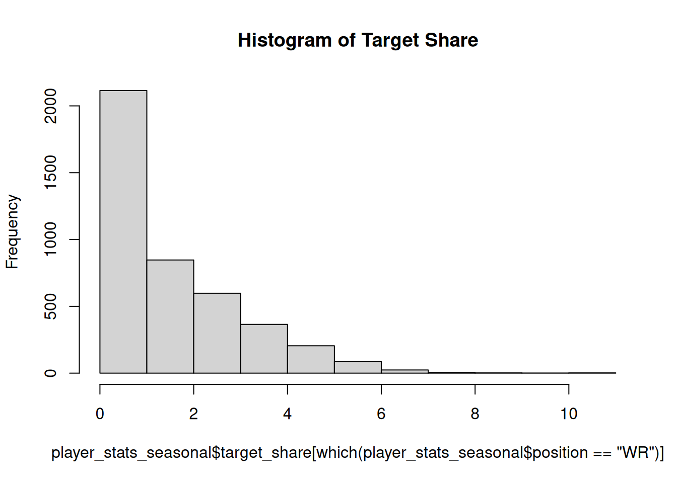
One approach we can take is to transform the target_shares variable to be more normally distributed.
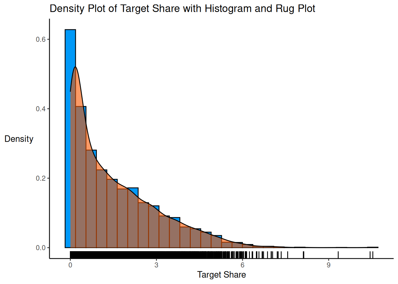
The histogram for the raw target_shares variable is in Figure 11.15.
Code
hist( player_stats_seasonal$target_share[which(player_stats_seasonal$position =="WR")],main ="Histogram of Target Share")
Figure 11.15: Histogram of Target Share.
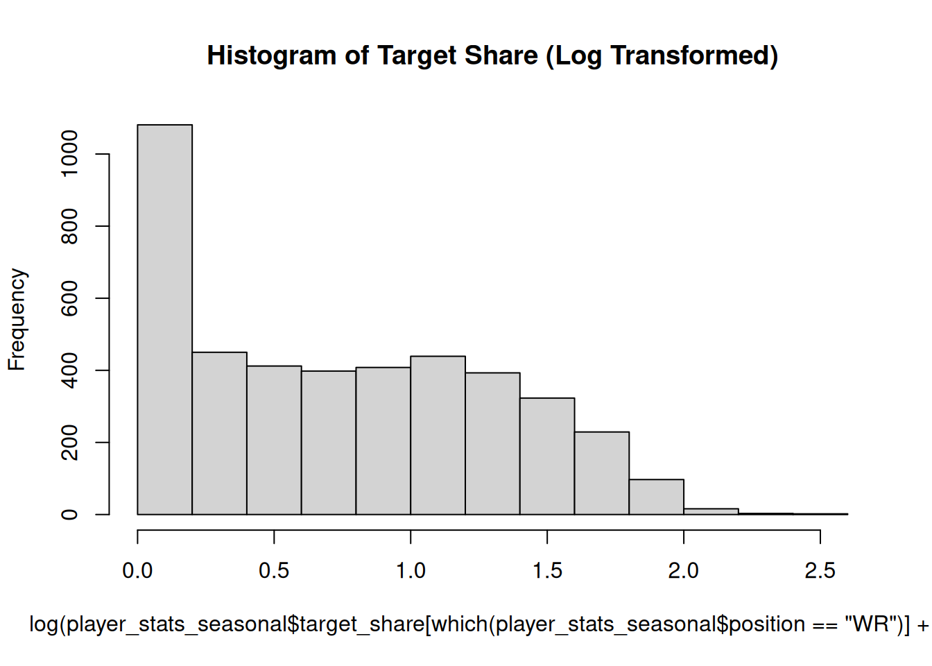
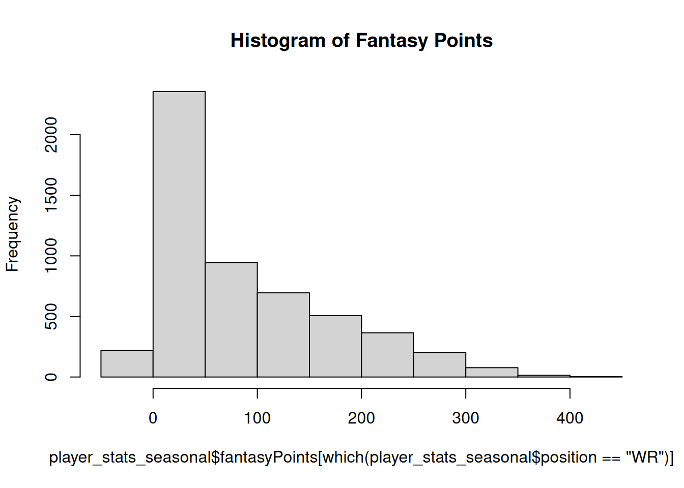
The variable shows a strong positive skew. To address a strong positive skew, we can use a log transformation. The histogram of the log-transformed variable is in Figure 11.16.
Code
hist(log(player_stats_seasonal$target_share[which(player_stats_seasonal$position =="WR")] +1),main ="Histogram of Target Share (Log Transformed)")
Figure 11.16: Histogram of Target Share, Transformed.
Now we can re-fit the model with the log-transformed variable.
Call:
lm(formula = fantasyPoints ~ age + I(age^2) + height + I(height^2) +
    weight + I(weight^2) + I(log(target_share + 1)), data = player_stats_seasonal %>%
    filter(position %in% c("WR")), na.action = "na.exclude")

Residuals:
    Min      1Q  Median      3Q     Max
-614.16  -15.28   -7.63    7.29  300.02

Coefficients:
                           Estimate Std. Error t value Pr(>|t|)
(Intercept)              -3.208e+02  4.751e+02  -0.675   0.4996
age                       3.227e+00  2.526e+00   1.278   0.2014
I(age^2)                 -4.931e-02  4.556e-02  -1.082   0.2791
height                    1.136e+01  1.403e+01   0.810   0.4181
I(height^2)              -8.050e-02  9.696e-02  -0.830   0.4065
weight                   -1.379e+00  8.803e-01  -1.567   0.1172
I(weight^2)               3.904e-03  2.190e-03   1.782   0.0748 .
I(log(target_share + 1))  9.030e+02  7.536e+00 119.827   <2e-16 ***
---
Signif. codes:  0 '***' 0.001 '**' 0.01 '*' 0.05 '.' 0.1 ' ' 1

Residual standard error: 40.87 on 4689 degrees of freedom
  (953 observations deleted due to missingness)
Multiple R-squared:  0.7623,    Adjusted R-squared:  0.762
F-statistic:  2149 on 7 and 4689 DF,  p-value: < 2.2e-16
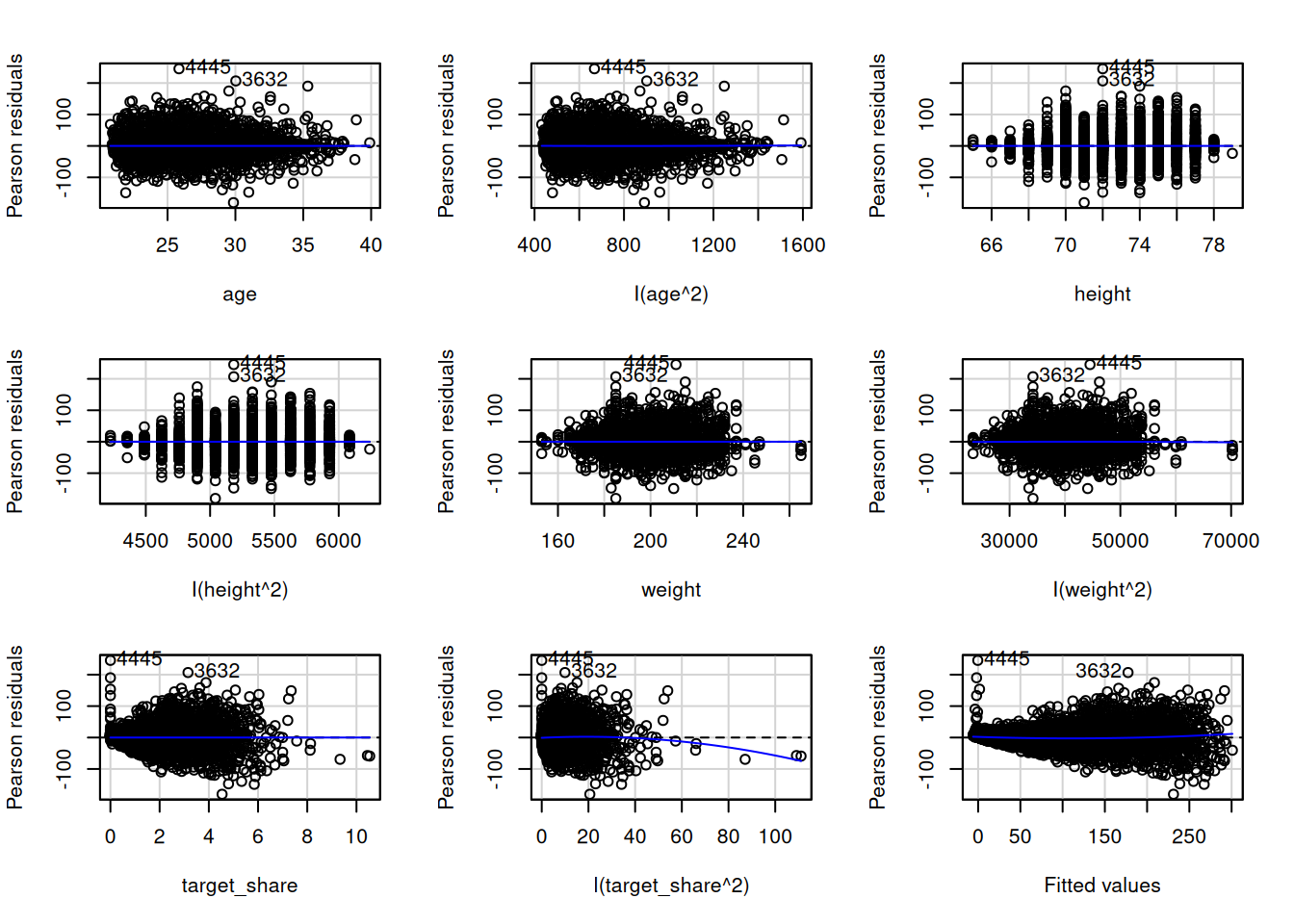
Target share shows a more linear association with fantasy points after log-transforming it (albeit still not perfect), as depicted in Figures 11.17, 11.18, 11.19, and 11.20.
Figure 11.20: Residual Plots After Log Transformation of Target Share.
11.10.8.2 Homoscedasticity
To evaluate homoscedasticity, we can evaluate a residual plot (Figure 11.21) and spread-level plot (Figure 11.22) from the car package (Fox et al., 2024; Fox & Weisberg, 2019). In a residual plot, you want a constant spread of residuals versus fitted values—you do not want the residuals to show a fan or cone shape.
In this example, the residuals appear to increase as a function of the fitted values. To handle this, we may need to transform the outcome variable to be more normally distributed.
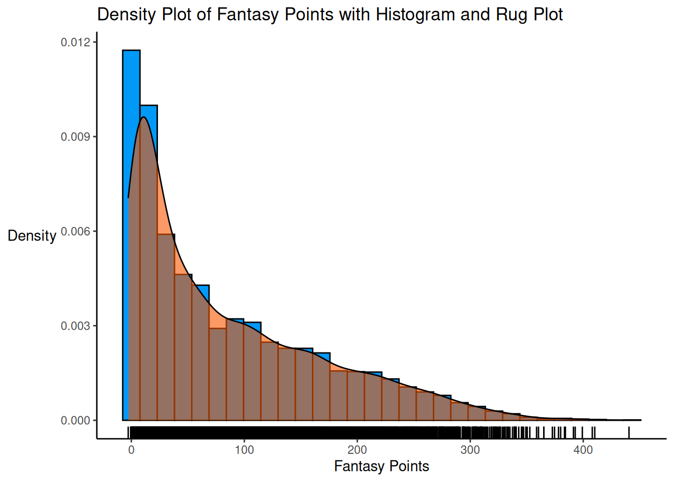
The histogram for raw fantasy points is in Figure 12.35.
Code
hist( player_stats_seasonal$fantasyPoints[which(player_stats_seasonal$position =="WR")],main ="Histogram of Fantasy Points")
Figure 11.23: Histogram of Fantasy Points (Among Wide Receivers).
Here are the transformation results—in this case, the best-fitting transformation is an ordered quantile (ORQ) normalization transformation:
Code
bnTransformed
Best Normalizing transformation with 42935 Observations
 Estimated Normality Statistics (Pearson P / df, lower => more normal):
 - arcsinh(x): 15.8276
 - Center+scale: 112.7684
 - Double Reversed Log_b(x+a): 158.3888
 - Exp(x): 79.5093
 - Log_b(x+a): 17.846
 - orderNorm (ORQ): 4.5967
 - sqrt(x + a): 39.3116
 - Yeo-Johnson: 8.5004
Estimation method: Out-of-sample via CV with 10 folds and 5 repeats

Based off these, bestNormalize chose:
orderNorm Transformation with 42935 nonmissing obs and ties
 - 5068 unique values
 - Original quantiles:
    0%    25%    50%    75%   100%
 -7.28   8.50  29.00  69.50 485.10
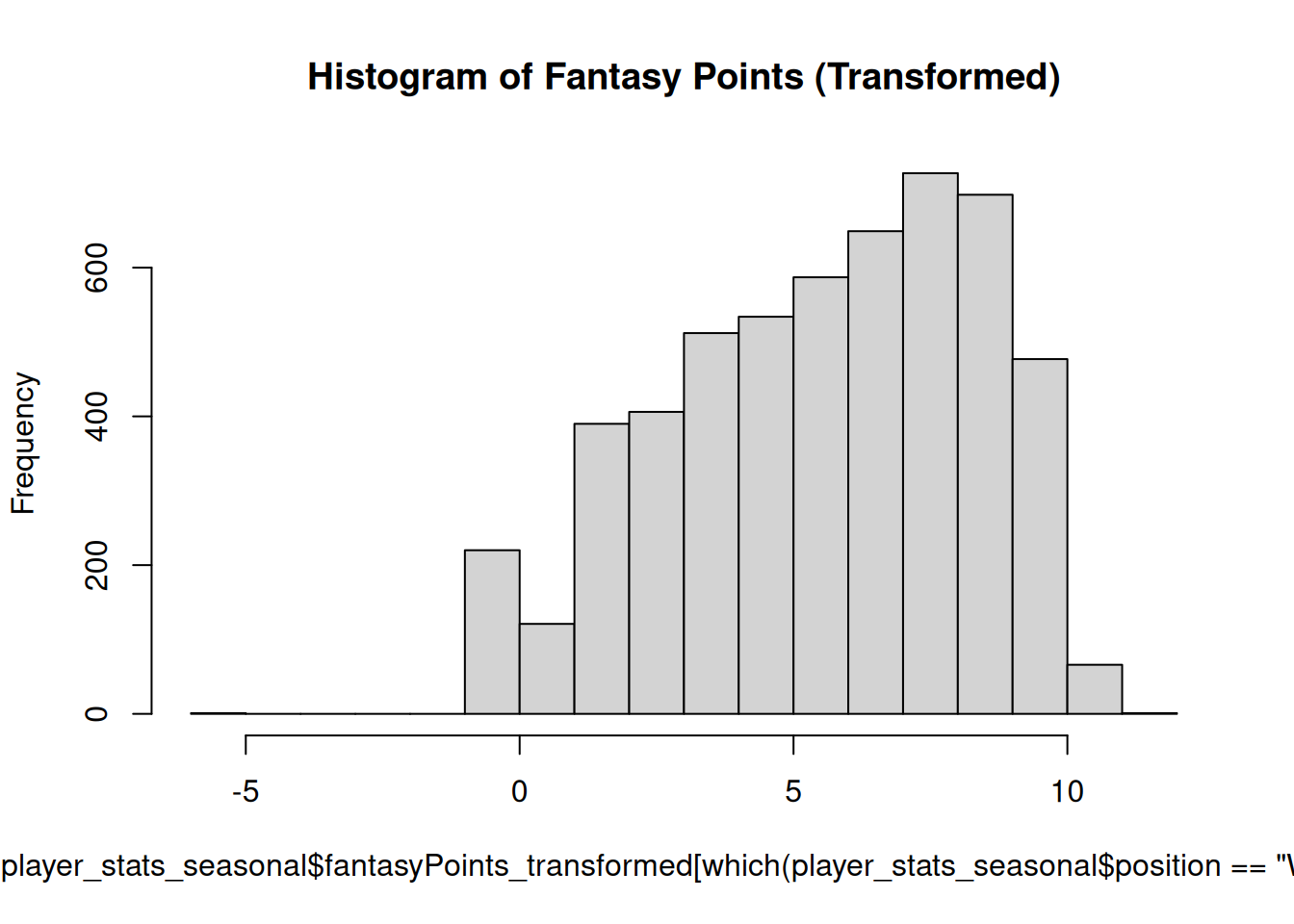
Then, we apply the best-fitting transformation to the variable, to create a transformed variable that is more normally distributed.
Code
player_stats_seasonal$fantasyPoints_transformed <-predict(bnTransformed)# Can back-transform transformed values back to the original metric later if needed:original <-predict( bnTransformed,newdata = player_stats_seasonal$fantasyPoints_transformed,inverse =TRUE)
The histogram of the transformed variable is in Figure 11.24.
Code
hist( player_stats_seasonal$fantasyPoints_transformed[which(player_stats_seasonal$position =="WR")],main ="Histogram of Fantasy Points (Transformed)")
Figure 11.24: Histogram of Fantasy Points (Among Wide Receivers), Transformed.
Figure 11.26: Spread-Level Plot After Transformation of Fantasy Points.
The residuals show more constant variance after transforming the outcome variable.
11.10.8.3 Uncorrelated Residuals
To determine if residuals are correlated given the nested structure of the data, we can examine the proportion of variance that is attributable to the particular player. To do this, we can estimate the intraclass correlation coefficient (ICC) from a mixed model using the performance package (Lüdecke et al., 2021; Lüdecke, Makowski, Ben-Shachar, Patil, Waggoner, et al., 2025).
The ICC indicates that over half of the variance is attribute to between-player variance, so it would be important to account for the player-specific variance using a mixed model. For simplicity, we focus on multiple regression models in this chapter; mixed models are described in Chapter 12.
11.10.8.4 Normally Distributed Residuals
We can examine whether residuals are normally distributed using quantile–quantile (QQ) plots and probability–probability (PP) plots, as in Figures 11.27 and 11.28. If the residuals are normally distributed, they should stay close to the diagonal reference line.
Figure 11.28: Residual Plots After Transformation of Fantasy Points.
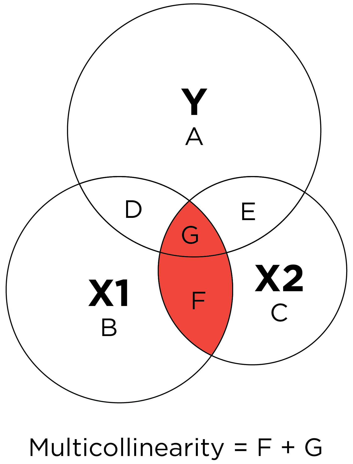
11.11 Multicollinearity
Multicollinearity occurs when two or more predictor variables in a regression model are highly correlated. The problem of having multiple predictor variables that are highly correlated is that it makes it challenging to estimate the regression coefficients accurately.
Multicollinearity in multiple regression is depicted conceptually in Figure 11.29.
Figure 11.29: Conceptual Depiction of Multicollinearity in Multiple Regression. From Petersen (2024) and Petersen (2025).
Table 11.3: Example Data of Predictors (x1 and x2) and Outcome (y) Used for Regression Model.
y
x1
x2
9
2.0
4
11
3.0
6
17
4.0
8
3
1.0
2
21
5.0
10
13
3.5
7
The second predictor variable is not very good—it is exactly twice the value of the first predictor variable; thus, the two predictor variables are perfectly correlated (i.e., \(r = 1.0\)). This means that there are different prediction equation possibilities that are equally good—see Equations in Equation 11.13:
\[
\begin{aligned}
2x_2 &= y \\
0x_1 + 2x_2 &= y \\
4x_1 &= y \\
4x_1 + 0x_2 &= y \\
2x_1 + 1x_2 &= y \\
5x_1 - 0.5x_2 &= y \\
...
&= y
\end{aligned}
\tag{11.13}\]
Then, what are the regression coefficients? We do not know what are the correct regression coefficients because each of the possibilities fits the data equally well. Thus, when estimating the regression model, we could obtain arbitrary estimates of the regression coefficients with an enormous standard error around each estimate. In general, multicollinearity increases the uncertainty (i.e., standard errors and confidence intervals) around the parameter estimates. Any predictor variables that have a correlation above ~ \(r = .30\) with each other could have an impact on the confidence interval of the regression coefficient. As the correlations among the predictor variables increase, the chance of getting an arbitrary answer increases, sometimes called “bouncing betas.” So, it is important to examine a correlation matrix of the predictor variables before putting them in the same regression model. You can also examine indices such as variance inflation factor (VIF), where a value greater than 5 or 10 indicates multicollinearity.
                     age                   height                   weight
                1.014639                 2.247440                 2.265154
I(log(target_share + 1))
                1.028635
To address multicollinearity, you can drop a redundant predictor or you can also use principal component analysis or factor analysis of the predictors to reduce the predictors down to a smaller number of meaningful predictors. For a meaningful answer regarding predictors in a regression framework that is precise and confident, you need a low level of intercorrelation among predictors, unless you have a very large sample size. However, if you are merely interested in prediction—and are not interested in interpreting the regression coefficients of individual predictors—multicollinearity poses less of a problem. For instance, machine learning cares more about achieving the greatest predictive accuracy possible and cares less about explaining which predictors are causally related to the outcome. So, multicollinearity is less of a concern for machine learning approaches.
An important consideration in multiple regression is how missing data are handled. Multiple regression in R using the stats::lm() function applies listwise deletion. Listwise deletion (also called complete case analysis) removes any row (in the data file) from analysis that has a missing value on the outcome variable or any of the predictor variables. Removing all rows from analysis that have any missingness in the model variables can be a problem because missingness is often not completely at random—missingness often occurs systematically (i.e., for a reason). For instance, participants may be less likely to have data for all variables if they are from a lower socioeconomic status background and do not have the time to participate in all study procedures. Thus, applying listwise deletion, we might systematically exclude participants from lower socioeconomic status backgrounds (or other groups), which could lead to less generalizable inferences.
It is thus important to consider approaches to handle missingness. Various approaches to handle missingness include pairwise deletion (aka available-case analysis), multiple imputation, and full information maximum likelihood (FIML).
11.13.1 Pairwise Deletion
Pairwise deletion (also called available case analysis) uses all available data for each pair of variables when estimating the correlations/covariances, and the resulting correlation/covariance matrix can be used to estimate a multiple regression model. We can estimate a regression model that uses pairwise deletion using the lavaan package (Rosseel, 2012; Rosseel et al., 2024).
lavaan 0.6-21 ended normally after 1 iteration

  Estimator                                         ML
  Optimization method                           NLMINB
  Number of model parameters                         6

  Number of observations                          4697

Model Test User Model:

  Test statistic                                 0.000
  Degrees of freedom                                 0

Parameter Estimates:

  Standard errors                             Standard
  Information                                 Expected
  Information saturated (h1) model          Structured

Regressions:
                              Estimate  Std.Err  z-value  P(>|z|)   Std.lv
  fantasyPoints_transformed ~
    age                          0.022    0.003    7.267    0.000    0.022
    height                       0.001    0.006    0.147    0.883    0.001
    weight                       0.002    0.001    2.347    0.019    0.002
    target_shar_lg              11.660    0.117   99.250    0.000   11.660
  Std.all

    0.059
    0.002
    0.028
    0.818

Intercepts:
                   Estimate  Std.Err  z-value  P(>|z|)   Std.lv  Std.all
   .fntsyPnts_trns   -1.598    0.327   -4.879    0.000   -1.598   -1.394

Variances:
                   Estimate  Std.Err  z-value  P(>|z|)   Std.lv  Std.all
   .fntsyPnts_trns    0.407    0.008   48.461    0.000    0.407    0.310

R-Square:
                   Estimate
    fntsyPnts_trns    0.690
11.13.2 Multiple Imputation
Multiple imputation takes a data set with missingness and it uses available information on other variables to estimate what likely values could have been for the missing value. It repeats the imputation multiple times, so there are multiple imputed data sets, which can give a sense of the degree of uncertainty of each imputed value. The model is then fit to each of the multiply imputed data sets separately, and the results are combined. We can multiply impute data using the mice package (van Buuren & Groothuis-Oudshoorn, 2011, 2024).
Now, let’s specify the imputation method—we use the two-level predictive mean matching (2l.pmm) method from the miceadds package (Robitzsch et al., 2024) to account for the nonindependent data (owing to multiple seasons per player):
Code
meth <- mice::make.method(dataToImpute)meth[1:length(meth)] <-""meth[Y] <-"2l.pmm"# specify the imputation method here; this can differ by outcome variable
Now, let’s specify the prediction matrix. A predictor matrix is a matrix of values, where:
rows with non-zero values are the target variables to be imputed
columns with non-zero values are predictors of the variable specified in the given row
the diagonal of the predictor matrix should be zero because a variable cannot predict itself
imp <- mice::mice(as.data.frame(dataToImpute),method = meth,predictorMatrix = pred,m = numImputations,maxit =5, # generally use 100 maximum iterations; this example uses 5 for speedseed =52242)
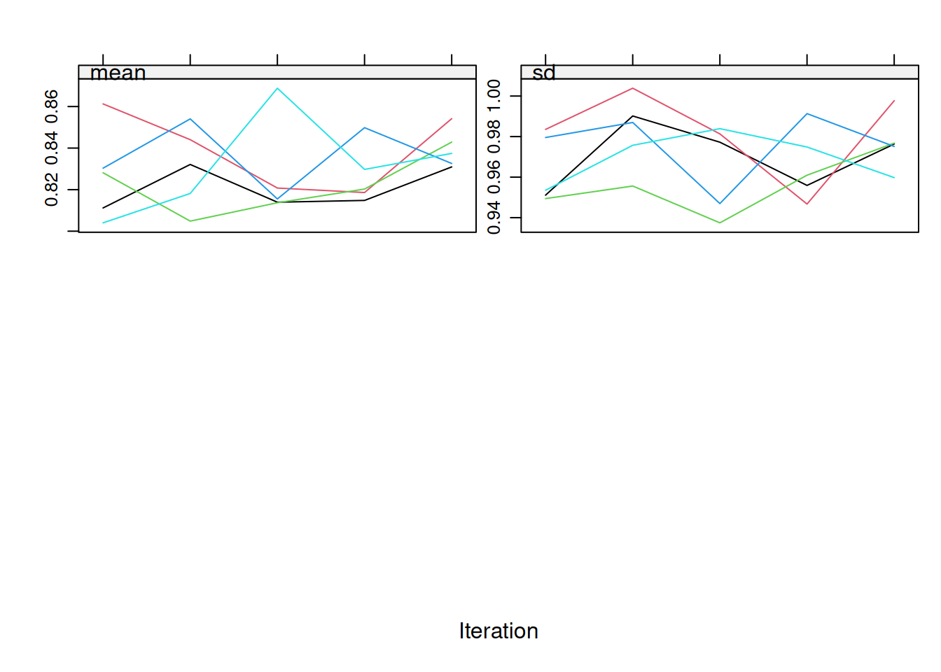
Below are some imputation diagnostics. Trace plots are in Figure 11.30.
Code
plot(imp, c("target_share"))
Figure 11.30: Trace plots from multiple imputation.
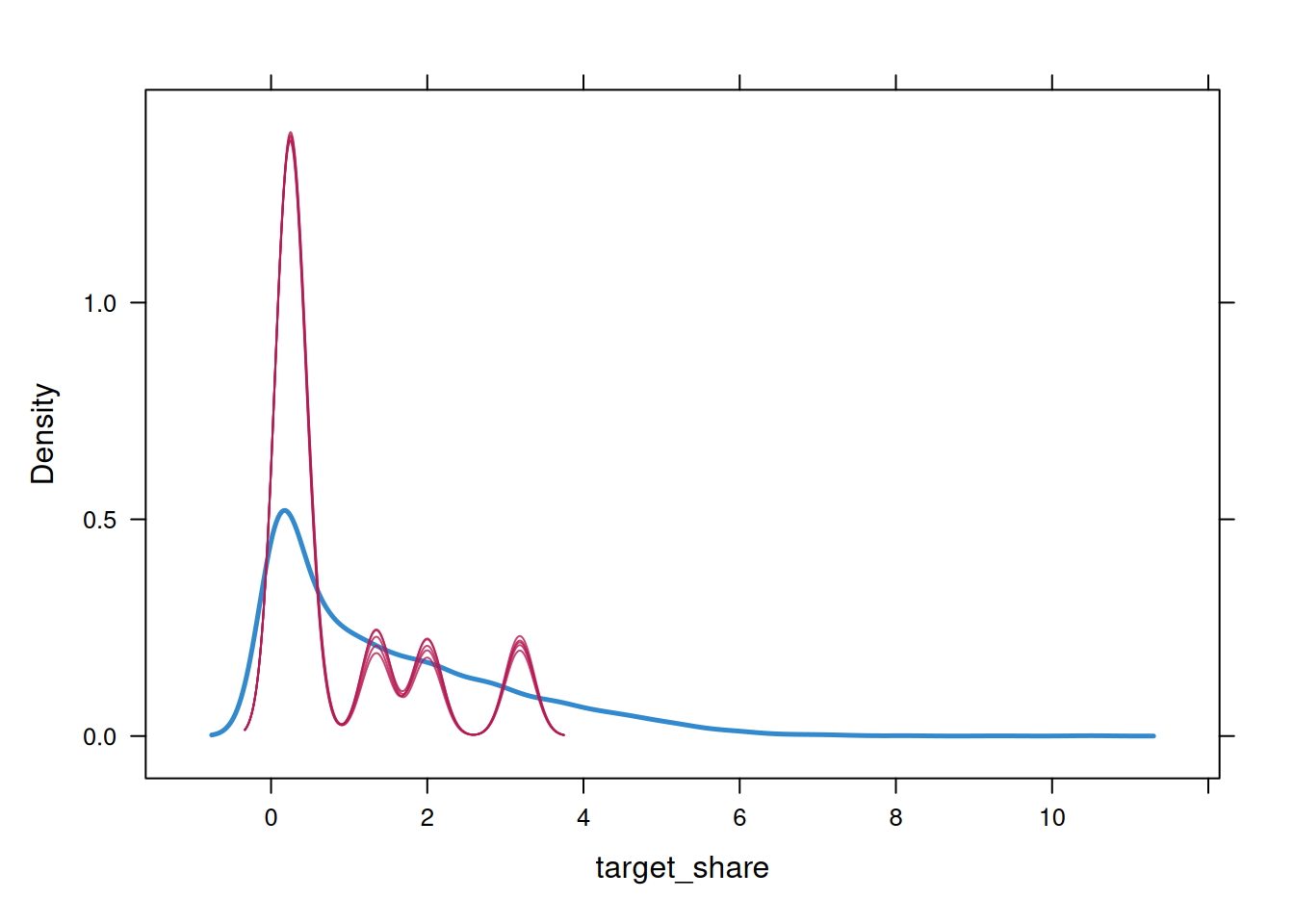
Figure 11.31: Density plot from multiple imputation.
The imputated data does not match well the distribution of the observed data. Thus, it may be necessary to select a different imputation method for more accurate imputation.
Error:
! arguments imply differing number of rows: 1, 0
Code
summary(mice::pool(imp_regression))
11.13.3 Full Information Maximum Likelihood
Full information maximum likelihood (FIML) estimates model parameters using all available data for each case, without imputing missing values. FIML is commonly used for handling missingness in approaches to latent variable modeling, such as factor analysis and structural equation modeling. We can estimate a regression model that uses full information maximum likelihood using the lavaan package (Rosseel, 2012; Rosseel et al., 2024).
lavaan 0.6-21 ended normally after 48 iterations

  Estimator                                         ML
  Optimization method                           NLMINB
  Number of model parameters                        20

  Number of observations                          5650
  Number of missing patterns                         2

Model Test User Model:

  Test statistic                                 0.000
  Degrees of freedom                                 0

Parameter Estimates:

  Standard errors                             Standard
  Information                                 Observed
  Observed information based on                Hessian

Regressions:
                              Estimate  Std.Err  z-value  P(>|z|)   Std.lv
  fantasyPoints_transformed ~
    age                          0.015    0.003    5.159    0.000    0.015
    height                      -0.002    0.006   -0.282    0.778   -0.002
    weight                       0.002    0.001    2.370    0.018    0.002
    target_shar_lg              11.683    0.113  102.952    0.000   11.683
  Std.all

    0.042
   -0.003
    0.028
    0.820

Covariances:
                   Estimate  Std.Err  z-value  P(>|z|)   Std.lv  Std.all
  age ~~
    height           -0.182    0.098   -1.860    0.063   -0.182   -0.025
    weight           -0.370    0.620   -0.597    0.551   -0.370   -0.008
    target_shar_lg    0.035    0.004    9.822    0.000    0.035    0.137
  height ~~
    weight           25.687    0.576   44.616    0.000   25.687    0.738
    target_shar_lg    0.016    0.003    6.149    0.000    0.016    0.085
  weight ~~
    target_shar_lg    0.149    0.016    9.033    0.000    0.149    0.124

Intercepts:
                   Estimate  Std.Err  z-value  P(>|z|)   Std.lv  Std.all
   .fntsyPnts_trns   -1.246    0.319   -3.909    0.000   -1.246   -1.087
    age              26.260    0.042  628.699    0.000   26.260    8.364
    height           72.558    0.031 2325.165    0.000   72.558   30.934
    weight          200.445    0.198 1014.698    0.000  200.445   13.499
    target_shar_lg    0.080    0.001   72.781    0.000    0.080    0.999

Variances:
                   Estimate  Std.Err  z-value  P(>|z|)   Std.lv  Std.all
   .fntsyPnts_trns    0.408    0.008   48.987    0.000    0.408    0.311
    age               9.857    0.185   53.150    0.000    9.857    1.000
    height            5.502    0.104   53.151    0.000    5.502    1.000
    weight          220.478    4.148   53.151    0.000  220.478    1.000
    target_shar_lg    0.006    0.000   50.486    0.000    0.006    1.000

R-Square:
                   Estimate
    fntsyPnts_trns    0.689
11.14 Addressing Non-Independence of Observations
Please note that the \(p\)-value for regression coefficients assumes that the observations are independent—in particular, that the residuals are not correlated. However, the observations are not independent in the player_stats_seasonal dataframe used above, because the same player has multiple rows—one row corresponding to each season they played. This non-independence violates the traditional assumptions of the significance of regression coefficients. We could address this assumption by analyzing only one season from each player or by estimating the significance of the regression coefficients using cluster-robust standard errors. For simplicity in the models above, we present results above from the whole dataframe. In Chapter 12, we discuss mixed model approaches that handle repeated measures and other data that violate assumptions of non-independence. Below, we demonstrate how to account for non-independence of observations using cluster-robust standard errors with the rms package (Harrell, Jr., 2025).
Code
player_stats_seasonal_subset <- player_stats_seasonal %>%filter(!is.na(player_id)) %>%filter(position %in%c("WR"))regressionWithClusterVariable <- rms::robcov(rms::ols( fantasyPoints_transformed ~ age + height + weight +I(log(target_share +1)),data = player_stats_seasonal_subset,x =TRUE,y =TRUE),cluster = player_stats_seasonal_subset$player_id) #account for nested data within playerregressionWithClusterVariable
Frequencies of Missing Values Due to Each Variable
fantasyPoints_transformed                       age                    height
                        0                         0                         0
                   weight              target_share
                        0                       953

Linear Regression Model

rms::ols(formula = fantasyPoints_transformed ~ age + height +
    weight + I(log(target_share + 1)), data = player_stats_seasonal_subset,
    x = TRUE, y = TRUE)

                                                      Model Likelihood    Discrimination
                                                            Ratio Test           Indexes
 Obs                                        4697    LR chi2    5471.11    R2       0.688
 sigma                                    0.6403    d.f.             4    R2 adj   0.688
 d.f.                                       4692    Pr(> chi2)  0.0000    g        1.014
Cluster onplayer_stats_seasonal_subset$player_id
 Clusters                                   1346

Residuals

    Min      1Q  Median      3Q     Max
-7.7389 -0.2298  0.0786  0.3290  3.0187

             Coef    S.E.   t     Pr(>|t|)
Intercept    -1.0336 0.4201 -2.46 0.0139
age           0.0124 0.0035  3.57 0.0004
height       -0.0032 0.0075 -0.43 0.6681
weight        0.0020 0.0011  1.85 0.0647
target_share 11.7152 0.4430 26.45 <0.0001
Call:
robustbase::lmrob(formula = fantasyPoints_transformed ~ age + height + weight +
    I(log(target_share + 1)), data = player_stats_seasonal %>% filter(position %in%
    c("WR")))
 \--> method = "MM"
Residuals:
     Min       1Q   Median       3Q      Max
-8.53606 -0.29144  0.01306  0.26351  3.08110

Coefficients:
                           Estimate Std. Error t value Pr(>|t|)
(Intercept)              -0.1835731  0.2275381  -0.807    0.420
age                      -0.0005275  0.0019637  -0.269    0.788
height                   -0.0067733  0.0041664  -1.626    0.104
weight                    0.0005558  0.0006472   0.859    0.391
I(log(target_share + 1)) 12.9061459  0.1075719 119.977   <2e-16 ***
---
Signif. codes:  0 '***' 0.001 '**' 0.01 '*' 0.05 '.' 0.1 ' ' 1

Robust residual standard error: 0.399
  (953 observations deleted due to missingness)
Multiple R-squared:  0.8474,    Adjusted R-squared:  0.8473
Convergence in 13 IRWLS iterations

Robustness weights:
 69 observations c(142,174,185,232,272,284,294,365,392,398,514,515,752,753,1117,1153,1173,1190,1191,1252,1307,1387,1388,1431,1508,1520,1572,1599,1637,1796,1884,2082,2279,2308,2325,2342,2361,2367,2404,2561,2586,2629,2741,2803,2838,2919,2953,2961,3100,3128,3311,3446,3456,3630,3713,3759,3760,3880,3881,3912,4007,4131,4146,4147,4271,4290,4391,4480,4622)
     are outliers with |weight| = 0 ( < 2.1e-05);
 392 weights are ~= 1. The remaining 4236 ones are summarized as
     Min.   1st Qu.    Median      Mean   3rd Qu.      Max.
0.0001167 0.8591000 0.9495000 0.8694000 0.9864000 0.9990000
Algorithmic parameters:
       tuning.chi                bb        tuning.psi        refine.tol
        1.548e+00         5.000e-01         4.685e+00         1.000e-07
          rel.tol         scale.tol         solve.tol          zero.tol
        1.000e-07         1.000e-10         1.000e-07         1.000e-10
      eps.outlier             eps.x warn.limit.reject warn.limit.meanrw
        2.129e-05         4.820e-10         5.000e-01         5.000e-01
     nResample         max.it         groups        n.group       best.r.s
           500             50              5            400              2
      k.fast.s          k.max    maxit.scale      trace.lev            mts
             1            200            200              0           1000
    compute.rd fast.s.large.n
             0           2000
                  psi           subsampling                   cov
           "bisquare"         "nonsingular"         ".vcov.avar1"
compute.outlier.stats
                 "SM"
seed : int(0)
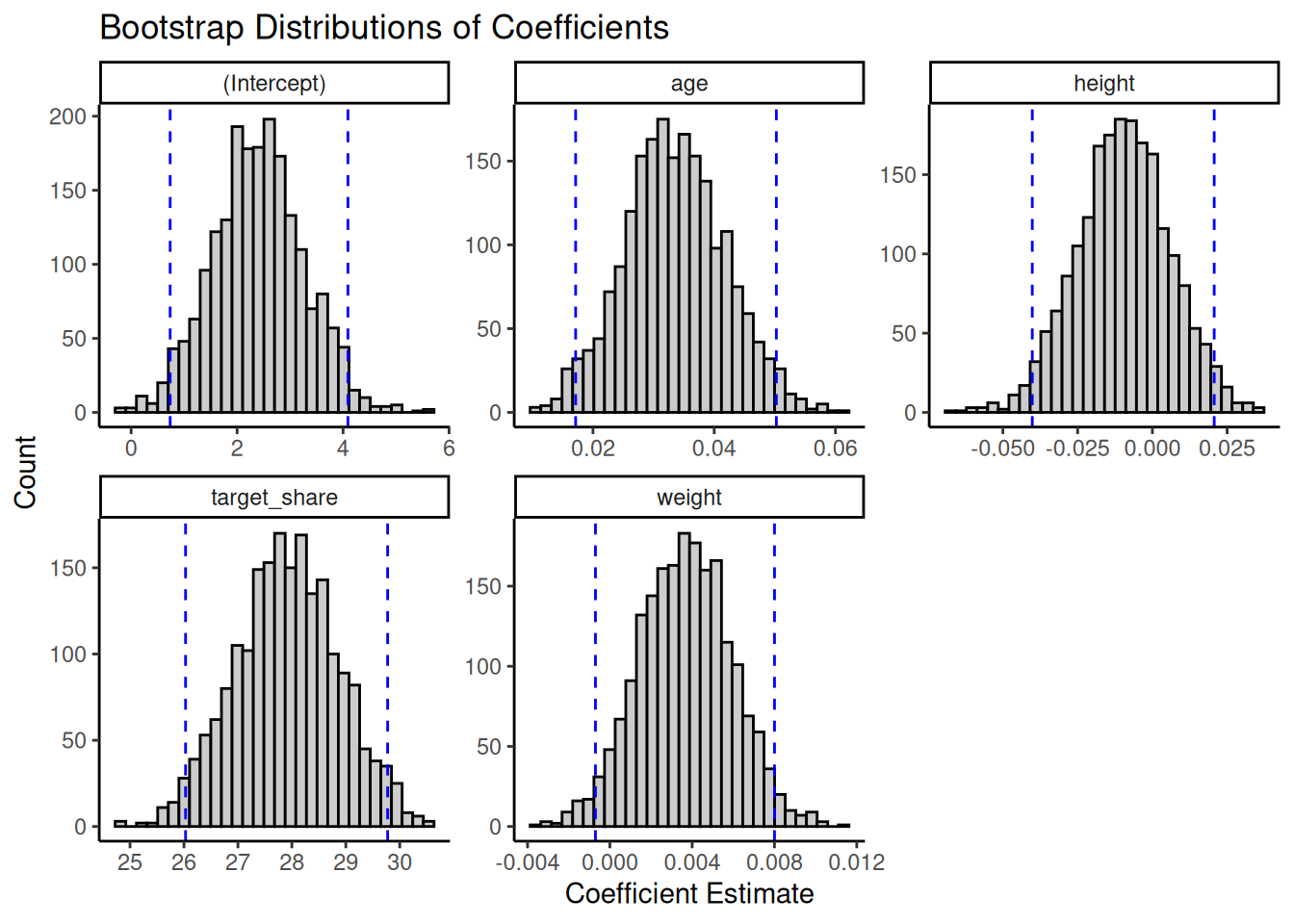
Another approach to handling outliers is to use boostrapping, which involves fitting models to various bootstrap resamples of the data. Bootstrap samples are datasets generated by sampling repeatedly with replacement.
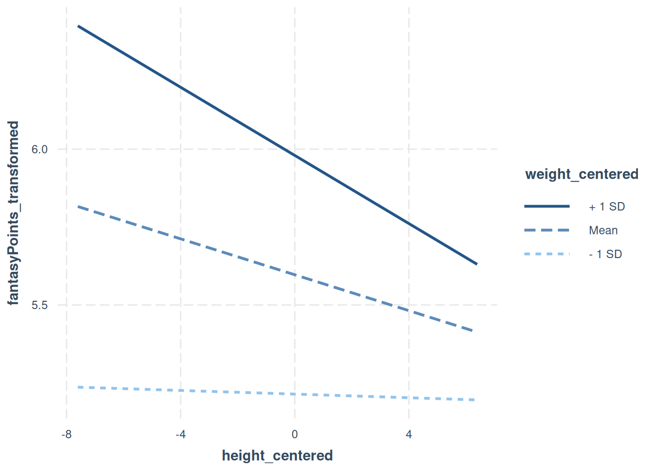
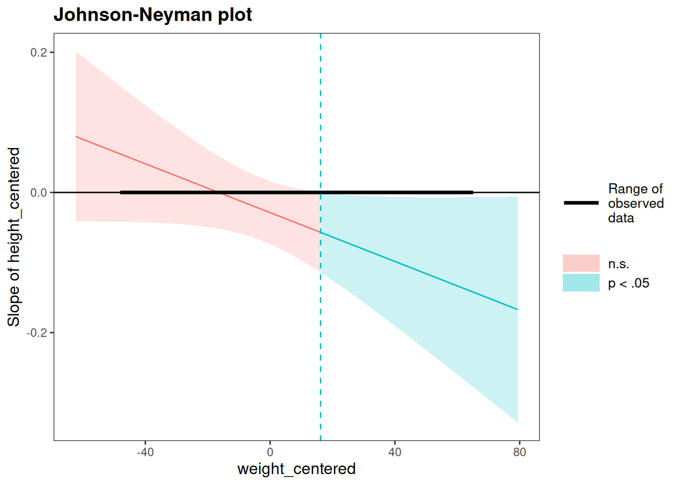
Now, we can visualize the interaction to understand it. We create an interaction plot (Figure 11.33) and Johnson-Neyman plot (Figure 11.34) using the interactions package (Long, 2024).
SIMPLE SLOPES ANALYSIS

Slope of height_centered when weight_centered = -1.484982e+01 (- 1 SD):

   Est.   S.E.   t val.      p
------- ------ -------- ------
  -0.00   0.01    -0.04   0.97

Slope of height_centered when weight_centered =  1.247537e-14 (Mean):

   Est.   S.E.   t val.      p
------- ------ -------- ------
  -0.01   0.01    -1.09   0.27

Slope of height_centered when weight_centered =  1.484982e+01 (+ 1 SD):

   Est.   S.E.   t val.      p
------- ------ -------- ------
  -0.02   0.01    -1.75   0.08
mediationModel <-' # direct effect (cPrime) Y ~ direct*X # mediator M ~ a*X Y ~ b*M # indirect effect = a*b indirect := a*b # total effect (c) total := direct + indirect totalAbs := abs(direct) + abs(indirect) # proportion mediated Pm := abs(indirect) / totalAbs'
Let’s substitute in our predictor, outcome, and hypothesized mediator. In this case, we predict that receiving touchdowns partially accounts for the association between Wide Receiver’s target share and their fantasy points. This is a silly example because fantasy points are derived, in part, from touchdowns, so of course touchdowns will partially account for almost any effect on Wide Receivers’ fantasy points. This example is merely for demonstrating the process of developing and examining a mediation model.
To get a robust estimate of the indirect effect, we obtain bootstrapped estimates from 1,000 bootstrap draws. Typically, we would obtain bootstrapped estimates from 10,000 bootstrap draws, but this example uses only 1,000 bootstrap draws for a shorter runtime.
Code
mediationFit <- lavaan::sem( mediationModel,data = player_stats_seasonal %>%filter(position %in%c("WR")),se ="bootstrap",bootstrap =1000, # generally use 10,000 bootstrap draws; this example uses 1,000 for speedparallel ="multicore", # parallelization for speed: use "multicore" for Mac/Linux; "snow" for PCiseed =52242, # for reproducibilitymissing ="ML",estimator ="ML",fixed.x =FALSE)
multipleMediatorFit <- lavaan::sem( multipleMediatorModel,data = player_stats_seasonal %>%filter(position %in%c("WR")),se ="bootstrap",bootstrap =1000, # generally use 10,000 bootstrap draws; this example uses 1,000 for speedparallel ="multicore", # parallelization for speed: use "multicore" for Mac/Linux; "snow" for PCiseed =52242, # for reproducibilitymissing ="ML",estimator ="ML",fixed.x =FALSE)
Error in `.fun()`:
! Boost not found; call install.packages('BH')
Code
summary(bayesianMultipleRegressionModel)
Error in `h()`:
! error in evaluating the argument 'object' in selecting a method for function 'summary': object 'bayesianMultipleRegressionModel' not found
Code
performance::r2(bayesianMultipleRegressionModel)
Error:
! object 'bayesianMultipleRegressionModel' not found
11.19 Conclusion
Multiple regression allows examining the association between multiple predictor variables and one outcome variable. Inclusion of multiple predictors in the model allows for potentially greater predictive accuracy and identification of the extent to which each variable uniquely contributes to the outcome variable. As with correlation, an association does not imply causation. However, identifying associations is important because associations are a necessary (but insufficient) condition for causality. When developing a multiple regression model, there are various assumptions that are important to evaluate. In addition, it is important to pay attention for potential multicollinearity—it may become difficult to detect a given predictor variable as statistically significant due to the greater uncertainty around the parameter estimates.
Ben-Shachar, M. S., Lüdecke, D., & Makowski, D. (2020). effectsize: Estimation of effect size indices and standardized parameters. Journal of Open Source Software, 5(56), 2815. https://doi.org/10.21105/joss.02815
Ben-Shachar, M. S., Makowski, D., Lüdecke, D., Patil, I., Wiernik, B. M., Thériault, R., & Waggoner, P. (2025). effectsize: Indices of effect size. https://doi.org/10.32614/CRAN.package.effectsize
Gaylord-Harden, N. K., Cunningham, J. A., Holmbeck, G. N., & Grant, K. E. (2010). Suppressor effects in coping research with African American adolescents from low-income communities. Journal of Consulting and Clinical Psychology, 78(6), 843–855. https://doi.org/10.1037/a0020063
Iacobucci, D., Schneider, M. J., Popovich, D. L., & Bakamitsos, G. A. (2016). Mean centering helps alleviate “micro” but not “macro” multicollinearity. Behavior Research Methods, 48(4), 1308–1317. https://doi.org/10.3758/s13428-015-0624-x
Lüdecke, D., Ben-Shachar, M. S., Patil, I., & Makowski, D. (2020). Extracting, computing and exploring the parameters of statistical models using R. Journal of Open Source Software, 5(53), 2445. https://doi.org/10.21105/joss.02445
Lüdecke, D., Ben-Shachar, M. S., Patil, I., Waggoner, P., & Makowski, D. (2021). performance: An R package for assessment, comparison and testing of statistical models. Journal of Open Source Software, 6(60), 3139. https://doi.org/10.21105/joss.03139
Lüdecke, D., Makowski, D., Ben-Shachar, M. S., Patil, I., Waggoner, P., Wiernik, B. M., & Thériault, R. (2025). performance: Assessment of regression models performance. https://doi.org/10.32614/CRAN.package.performance
MacKinnon, D., Krull, J., & Lockwood, C. (2000). Equivalence of the mediation, confounding and suppression effect. Prevention Science, 1(4), 173–181. https://doi.org/10.1023/A:1026595011371
Petersen, I. T. (2024). Principles of psychological assessment: With applied examples in R. Chapman and Hall/CRC. https://doi.org/10.1201/9781003357421
Petersen, I. T. (2025). Principles of psychological assessment: With applied examples in R. University of Iowa Libraries. https://doi.org/10.25820/work.007199
Peterson, R. A. (2021). Finding optimal normalizing transformations via bestNormalize. The R Journal, 13(1), 310–329. https://doi.org/10.32614/RJ-2021-041
Peterson, R. A., & Cavanaugh, J. E. (2020). Ordered quantile normalization: A semiparametric transformation built for the cross-validation era. Journal of Applied Statistics, 47(13-15), 2312–2327. https://doi.org/10.1080/02664763.2019.1630372
Rosseel, Y. (2012). lavaan: An R package for structural equation modeling. Journal of Statistical Software, 48(2), 1–36. https://doi.org/10.18637/jss.v048.i02
Todorov, V., & Filzmoser, P. (2009). An object-oriented framework for robust multivariate analysis. Journal of Statistical Software, 32(3), 1–47. https://doi.org/10.18637/jss.v032.i03
van Buuren, S., & Groothuis-Oudshoorn, K. (2011). mice: Multivariate imputation by chained equations in R. Journal of Statistical Software, 45(3), 1–67. https://doi.org/10.18637/jss.v045.i03
Please consider providing feedback about this textbook, so that I can make it as helpful as possible. You can provide feedback at the following link:
https://forms.gle/LsnVKwqmS1VuxWD18
Email Notification
The online version of this book will remain open access. If you want to know when the print version of the book is for sale, enter your email below so I can let you know.