I want your feedback to make the book better for you and other readers. If you find typos, errors, or places where the text may be improved, please let me know. The best ways to provide feedback are by GitHub or hypothes.is annotations.
You can leave a comment at the bottom of the page/chapter, or open an issue or submit a pull request on GitHub: https://github.com/isaactpetersen/Fantasy-Football-Analytics-Textbook
Alternatively, you can leave an annotation using hypothes.is.
To add an annotation, select some text and then click the
symbol on the pop-up menu.
To see the annotations of others, click the
symbol in the upper right-hand corner of the page.
26 Decision Making in the Context of Uncertainty
This chapter provides an overview of various considerations in judgment and decision making in the context of uncertainty.
26.1 Getting Started
26.1.1 Load Packages
26.1.2 Load Data
We created the projectionsWithActuals_seasonal.RData object in Section 17.1.4.1; we created the projectionsWithActuals_weekly.RData object in Section 17.1.4.2. We created the player_stats_weekly.RData and player_stats_seasonal.RData objects in Section 4.4.3.
26.2 Overview of Decision Making in Uncertainty
26.3 Wisdom of the Crowd
In many domains, the average of forecasters’ predictions is more accurate than the accuracy of the constituent individuals. In some domains, the average of non-expert forecasts is more accurate than the forecasts by individual experts. This phenomenon is called “collective intelligence”, the “wisdom of the crowd”, or the “wisdom of crowds” (Larrick et al., 2024; Rader et al., 2017; Simoiu et al., 2019; Surowiecki, 2005; Wagner & Vinaimont, 2010).
Aggregation of predictions from multiple people leverages several important features, including cognitive diversity and error cancellation. Cognitive diversity refers to the representation of individuals with different perspectives because of their “differences in knowledge, training, experience, or thinking styles” (Rader et al., 2017, p. 8). Cognitive diversity is important because judgments from a cognitively homogeneous group will tend to err systematically. That is, they tend to err in the same direction—either consistently above or below the truth; thus, their errors are correlated. By contrast, a cognitively diverse group will not tend to err systematically. Individuals of a cognitively diverse group will bring different areas of expertise (e.g., determination of player skill, player opportunity, matchup strength, etc.) to bear in making their predictions and will thus make different mistakes (Larrick et al., 2024). Consequently, for the people comprising a cognitively diverse group, their judgments will tend to err randomly—where some people’s predictions fall above the truth and some people’s predictions fall below the truth—i.e., individual judgments “bracket” the truth (Mannes et al., 2014). Thus, judgments from a cognitively diverse group tend to have uncorrelated errors.
Error cancellation deals with the idea that, when individuals’ judgments bracket the truth and show random rather than systematic error, the average of the predictions will “cancel out” some of the errors so that the predictions average out to more closely approximate the truth. However, when individuals’ judgments do not bracket the truth, the average of the predictions will not cancel out the errors.
Averaging projections from individuals tends to yield predictions that are more accurate than the accuracy of most forecasters in the group (Mannes et al., 2014). Indeed, when at least some of the projections bracket the truth, averaged predictions must be more accurate than the average individual forecaster—in terms of mean absolute error (MAE)—and averaged predictions are often much more accurate (Larrick et al., 2024). When referring to the accuracy of the “average individual forecaster”, we are referring to accuracy in terms of mean absolute error (MAE)—not to the accuracy of the forecaster at the 50th percentile. If none of the projections bracket the truth—e.g., all projections overestimate the truth—averaged predictions will be as accurate as the average individual forecaster in terms of mean absolute error (Larrick et al., 2024). In sum, “Averaging the answers of a crowd, therefore, ensures a level of accuracy no worse than the average member of the crowd and, in some cases, a level better than nearly all members” (Larrick et al., 2024, p. 126). Moreover, averaged projections tend to be more accurate than consensus-based judgments from groups of people that interact and discuss, due to cognitive biases associated with the social interaction among groups, such as herding in which people align their behavior with others (Mannes et al., 2014; Simoiu et al., 2019), though discussion can be helpful in some contexts (Larrick et al., 2024).
There are well-known prediction markets, in which people bet money to make predictions for various events, which allows determining the crowd-averaged prediction for events:
There are also betting markets for football:
- https://www.rotowire.com/betting/nfl/player-futures.php
- https://vegasprojections.com
- https://www.actionnetwork.com/nfl/props
- https://tools.32beatwriters.com
- https://the-odds-api.com
- https://www.evsharps.com/ranks?format=std
Crowd-averaged projections tend to be most accurate when:
- the crowd consists of individuals who hold expertise in the domain such that they will make predictions that fall close to the truth
- there is relatively low variability in the expertise of the individual forecasters in terms of their ability to make accurate forecasts
- there is cognitive diversity among the forecasters
- the projections are made independently—i.e., the forecasters are not aware of others’ forecasts and do not discuss or interact with the other forecasters
- the bracketing rate—i.e., the frequency with which any two forecasters’ predictions fall on opposite sides of the truth—is high
- there are at least 5–10 sources of projections
However, the crowd is not more accurate than the expert or best forecaster in all situations or domains. For instance, the crowd tends to be less accurate than the (prospectively identified) best forecaster when there is great variability in forecasters’ expertise (in terms of the forecasters’ ability to forecast accurately) and when the bracketing rate is low (Mannes et al., 2014). Some forecasters may provide terrible projections; thus, including them in an average may make the average projections substantially less accurate. Thus, it may be necessary to examine the average of a “select crowd”, by aggregating the projections of the most consistently accurate forecasters (Mannes et al., 2014). Incorporating at least 5–10 forecasters leverages most of the benefits of the crowd; adding additional forecasters tends to result in diminishing returns (Larrick et al., 2024). However, to the extent that those who are most accurate in a given period reflects luck, you are better off averaging the predictions of all forecasters than selecting the forecasters who were most accurate in the most recent period (Larrick et al., 2024).
26.4 Accuracy of Fantasy Football Crowd Projections
Even though the crowd tends to be more accurate than individual forecasters (Kartes, 2024; archived at https://perma.cc/69F7-LLTN; Petersen, 2017; archived at https://perma.cc/BG2W-ANUF), crowd-averaged projections (at least among experts) are not necessarily highly accurate, as described in Section 17.12.3. In fantasy football, crowd-averaged seasonal projections explain ~60–75% of the variance in fantasy points among offensive players; however, the percent of variance explained drops to ~30% when considering only those players with high projected or actual points—who are the players that are the most important to distinguish, because those are the players that you are most likely trying to decide between when drafting. Nevertheless, individual sources tend to be even less accurate. Individual projections sources tend to explain ~50–65% of the variance in fantasy points among offensive players; however, the percent of variance explained also drops considerably when considering only those players with high projected or actual points.
The petersenlab package (Petersen, 2025) has the petersenlab::wisdomOfCrowd() function that computes the overall accuracy of the crowd-averaged projections, including the bracketing rate of the individual projections.
26.4.1 Examples
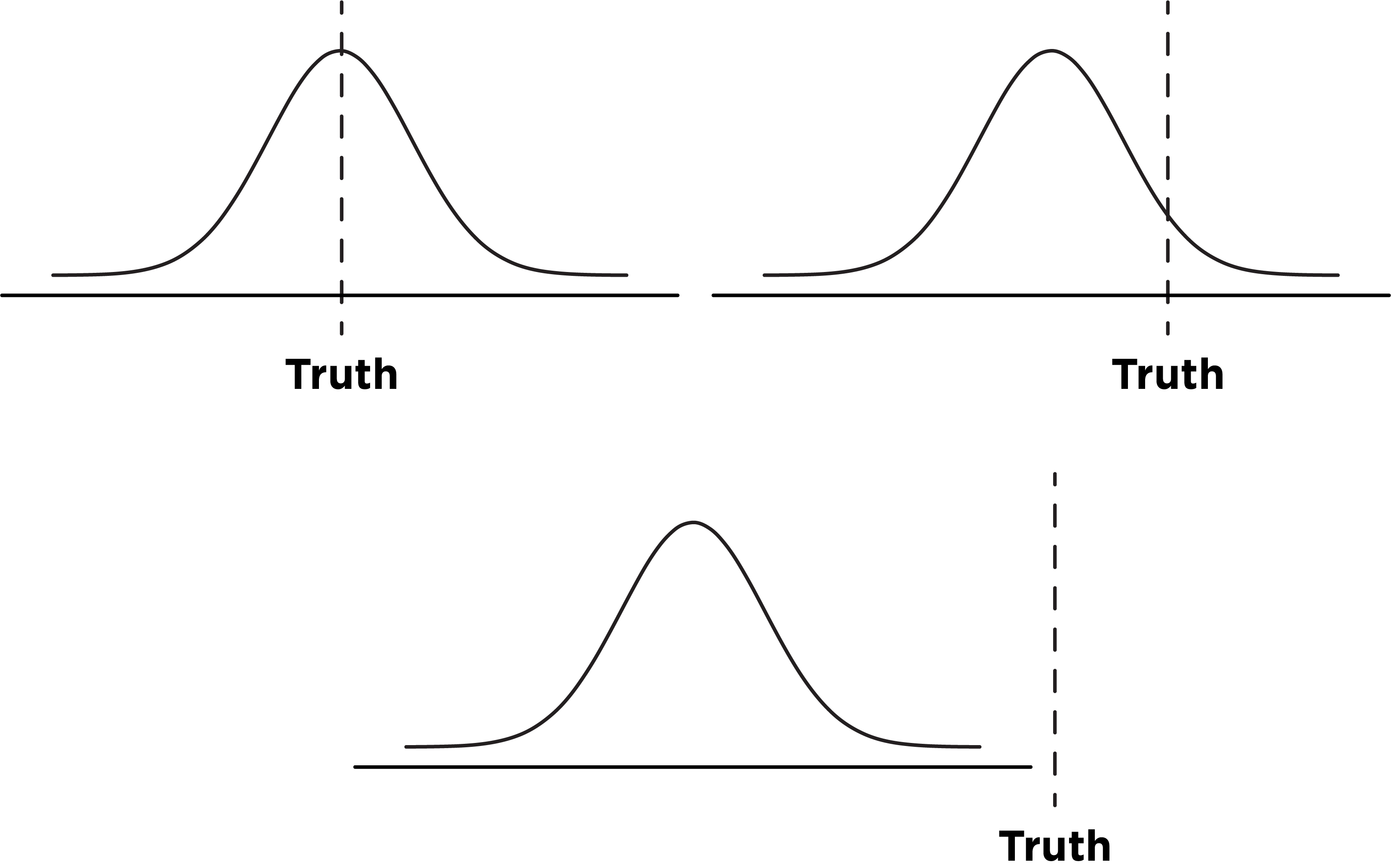
Below are examples where the predictions a) are centered on the truth, b) bracket the truth, and c) do not bracket the truth. They are illustrated in Figure 26.1.
Here is a code example of when the individual predictions (from which the crowd-averaged predictions are derived) are centered on the truth for a player. The distribution of projected points versus truth is depicted in Figure 26.2.
Code
[1] -40 -30 -20 -10 10 20 30 40[1] 50Code
bracketingCentered <- petersenlab::wisdomOfCrowd(
  predicted = predictedValues,
  actual = actualValue
)

bracketingCentered_bracketingRate <- bracketingCentered[which(row.names(bracketingCentered) == "crowdAveraged"), "bracketingRate"] * 100

maeBracketingCentered_individual <- bracketingCentered[which(row.names(bracketingCentered) == "individual"), "MAE"]
maeBracketingCentered_crowd <- bracketingCentered[which(row.names(bracketingCentered) == "crowdAveraged"), "MAE"]

mdaeBracketingCentered_individual <- bracketingCentered[which(row.names(bracketingCentered) == "individual"), "MdAE"]
meBracketingCentered_crowd <- bracketingCentered[which(row.names(bracketingCentered) == "crowdAveraged"), "ME"]

ggplot2::ggplot(,
  mapping = aes(
    x = predictedValues)
) +
  geom_density(
    fill = "lightgray"
  ) +
  geom_vline(
    xintercept = mean(predictedValues),
    color = "darkgray",
    linewidth = 1.5) +
    geom_vline(
    xintercept = actualValue,
    linetype = "dashed",
    linewidth = 1.5
  ) +
  #annotate(
  #  "segment",
  #  x = mean(predictedValues),
  #  xend = actualValue,
  #  y = 0,
  #  yend = 0,
  #  linewidth = 1.5,
  #  arrow = arrow(
  #    angle = 20,
  #    ends = "both",
  #    type = "closed")
  #)
  annotate(
    "text",
    x = mean(predictedValues) + (maeBracketingCentered_crowd / 2) + 1,
    y = 0.0003,
    label = paste("Mean Error: ", meBracketingCentered_crowd, sep = ""),
    hjust = 0 # left-justify
  ) +
  labs(
    x = "Fantasy Points",
    y = "Density",
    title = "Density Plot of Predicted Fantasy Points for a Player",
    subtitle = "Crowd-Averaged Projection (Vertical Gray Line) Vs.\nTruth, i.e., Actual Fantasy Points (Dashed Line)"
  ) +
  theme_classic() +
  theme(axis.title.y = element_text(angle = 0, vjust = 0.5)) # horizontal y-axis title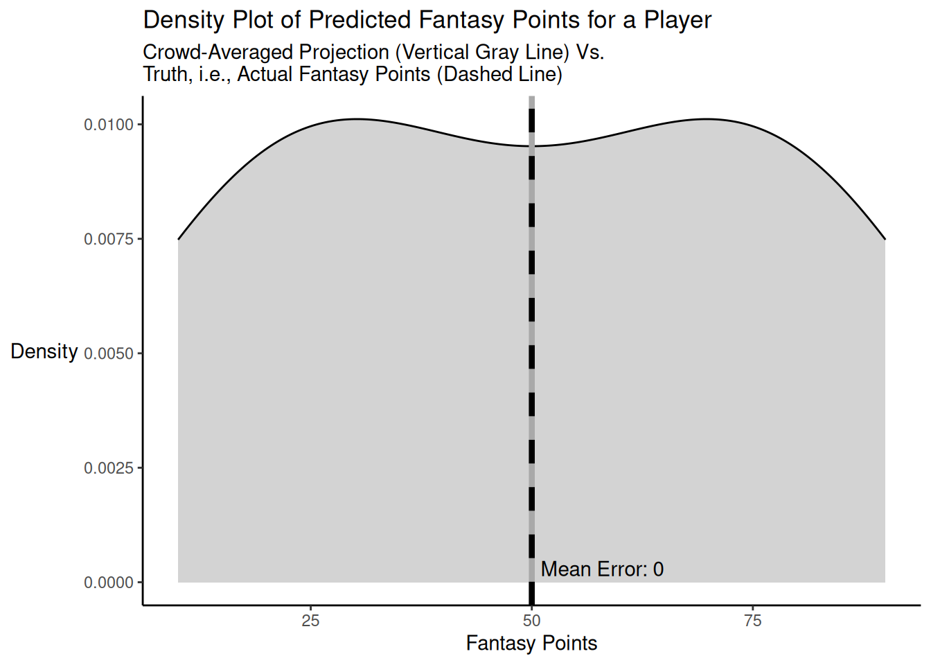
As demonstrated above, when the individual predictions are centered on the truth, the bracketing rate is very high (in this case, 57.14%), and the crowd-averaged predictions are perfectly accurate and are more accurate (MAE/MdAE = 0) than the accuracy of the typical individual forecaster (MAE = 25; MdAE = 25) in terms of mean absolute error and median absolute error.
Here is a code example of when the individual predictions bracket but are not centered on the truth for a player, with a high bracketing rate and no strong outliers. The distribution of projected points versus truth is depicted in Figure 26.3.
Code
[1] -61 -42 -42 -31 -11 -1 9 19[1] 51Code
bracketingNotCentered1 <- petersenlab::wisdomOfCrowd(
  predicted = predictedValues,
  actual = actualValue
)

bracketingNotCentered1_bracketingRate <- bracketingNotCentered1[which(row.names(bracketingNotCentered1) == "crowdAveraged"), "bracketingRate"] * 100

maeBracketingNotCentered1_individual <- bracketingNotCentered1[which(row.names(bracketingNotCentered1) == "individual"), "MAE"]
maeBracketingNotCentered1_crowd <- bracketingNotCentered1[which(row.names(bracketingNotCentered1) == "crowdAveraged"), "MAE"]

mdaeBracketingNotCentered1_individual <- bracketingNotCentered1[which(row.names(bracketingNotCentered1) == "individual"), "MdAE"]
meBracketingNotCentered1_crowd <- bracketingNotCentered1[which(row.names(bracketingNotCentered1) == "crowdAveraged"), "ME"]

ggplot2::ggplot(,
  mapping = aes(
    x = predictedValues)
) +
  geom_density(
    fill = "lightgray"
  ) +
  geom_vline(
    xintercept = mean(predictedValues),
    color = "darkgray",
    linewidth = 1.5) +
    geom_vline(
    xintercept = actualValue,
    linetype = "dashed",
    linewidth = 1.5
  ) +
  annotate(
    "segment",
    x = mean(predictedValues),
    xend = actualValue,
    y = 0,
    yend = 0,
    linewidth = 1.5,
    arrow = arrow(
      angle = 20,
      ends = "both",
      type = "closed")
  ) +
  annotate(
    "text",
    x = actualValue + (meBracketingNotCentered1_crowd / 2),
    y = 0.0007,
    label = paste("Mean Error: ", meBracketingNotCentered1_crowd, sep = ""),
    hjust = 0.5 # center-justify
  ) +
  labs(
    x = "Fantasy Points",
    y = "Density",
    title = "Density Plot of Predicted Fantasy Points for a Player",
    subtitle = "Crowd-Averaged Projection (Vertical Gray Line) Vs.\nTruth, i.e., Actual Fantasy Points (Dashed Line)"
  ) +
  theme_classic() +
  theme(axis.title.y = element_text(angle = 0, vjust = 0.5)) # horizontal y-axis title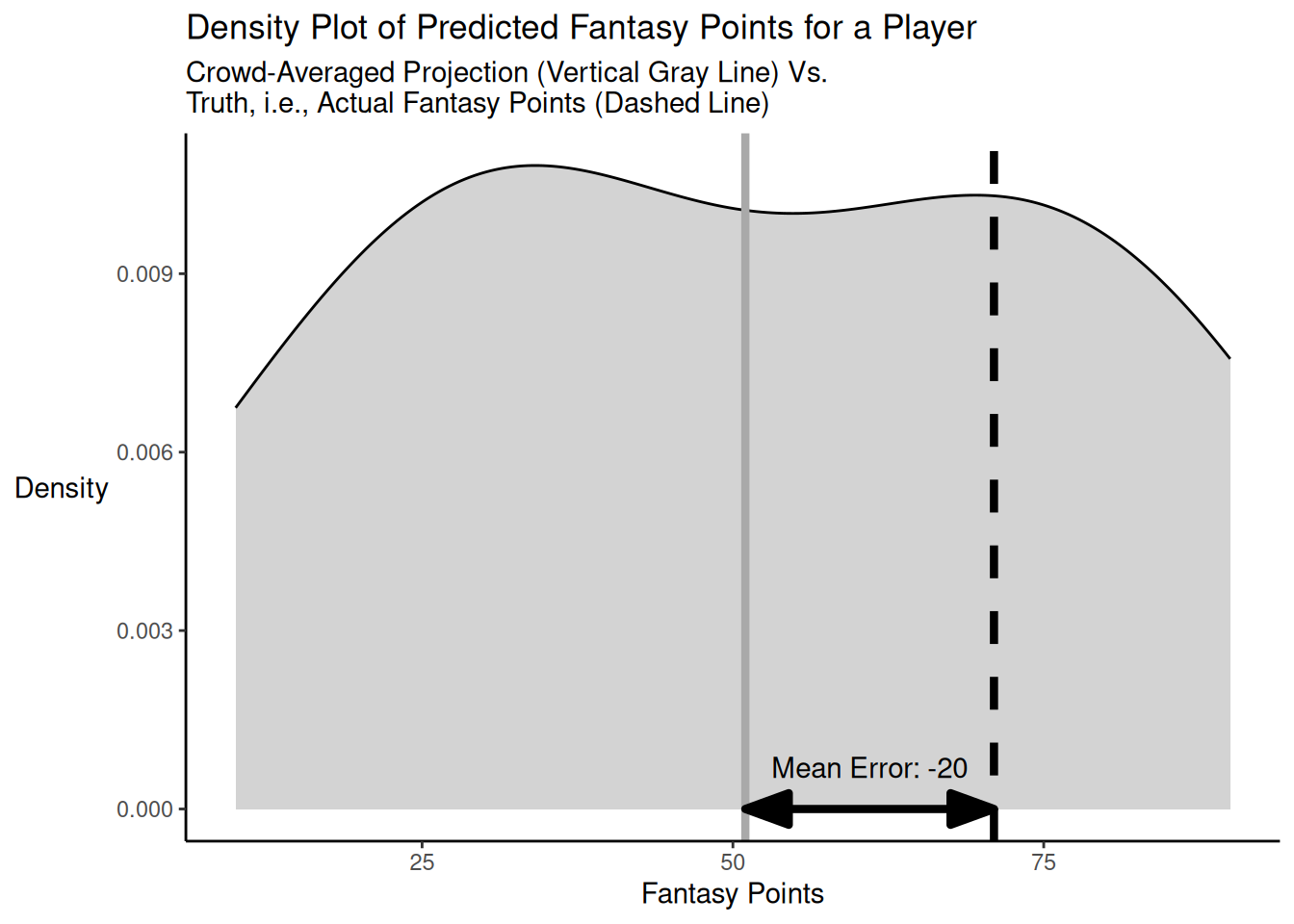
As demonstrated above, when the individual predictions bracket but are not centered on the truth, and the bracketing rate is high (in this case, 42.86%) with no strong outliers, the crowd-averaged predictions (MAE/MdAE = 20) are more accurate than the accuracy of the typical individual forecaster (MAE = 27; MdAE = 25) in terms of mean absolute error and median absolute error.
Here is a code example of when the individual predictions bracket but are not centered on the truth for a player, with a high bracketing rate but with an outlier projection that is far away from the truth. The distribution of projected points versus truth is depicted in Figure 26.4.
Code
[1] -34 -14 -4 6 16 26 36 176[1] 100Code
bracketingnotCentered2 <- petersenlab::wisdomOfCrowd(
  predicted = predictedValues,
  actual = actualValue
)

bracketingnotCentered2_bracketingRate <- bracketingnotCentered2[which(row.names(bracketingnotCentered2) == "crowdAveraged"), "bracketingRate"] * 100

maeBracketingnotCentered2_individual <- bracketingnotCentered2[which(row.names(bracketingnotCentered2) == "individual"), "MAE"]
maeBracketingnotCentered2_crowd <- bracketingnotCentered2[which(row.names(bracketingnotCentered2) == "crowdAveraged"), "MAE"]

mdaeBracketingnotCentered2_individual <- bracketingnotCentered2[which(row.names(bracketingnotCentered2) == "individual"), "MdAE"]
meBracketingnotCentered2_crowd <- bracketingnotCentered2[which(row.names(bracketingnotCentered2) == "crowdAveraged"), "ME"]

ggplot2::ggplot(,
  mapping = aes(
    x = predictedValues)
) +
  geom_density(
    fill = "lightgray"
  ) +
  geom_vline(
    xintercept = mean(predictedValues),
    color = "darkgray",
    linewidth = 1.5) +
    geom_vline(
    xintercept = actualValue,
    linetype = "dashed",
    linewidth = 1.5
  ) +
  annotate(
    "segment",
    x = mean(predictedValues),
    xend = actualValue,
    y = 0,
    yend = 0,
    linewidth = 1.5,
    arrow = arrow(
      angle = 20,
      ends = "both",
      type = "closed")
  ) +
  annotate(
    "text",
    x = actualValue + (meBracketingnotCentered2_crowd / 2),
    y = 0.0007,
    label = paste("Mean Error: ", meBracketingnotCentered2_crowd, sep = ""),
    hjust = 0.5 # center-justify
  ) +
  labs(
    x = "Fantasy Points",
    y = "Density",
    title = "Density Plot of Predicted Fantasy Points for a Player",
    subtitle = "Crowd-Averaged Projection (Vertical Gray Line) Vs.\nTruth, i.e., Actual Fantasy Points (Dashed Line)"
  ) +
  theme_classic() +
  theme(axis.title.y = element_text(angle = 0, vjust = 0.5)) # horizontal y-axis title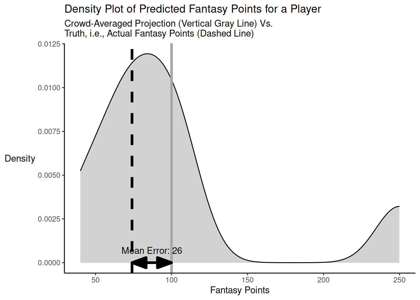
As demonstrated above, when the individual predictions bracket but are not centered on the truth, and the bracketing rate is high (in this case, 53.57%) but with an outlier projection that is far away from the truth, the crowd-averaged predictions (MAE/MdAE = 26) are more accurate than the accuracy of the typical individual forecaster (MAE = 39) in terms of mean absolute error, but they can still be less accurate—in terms of median absolute error—than the individual forecaster who is at the 50th percentile in accuracy (MdAE = 21).
Here is another code example of when the individual predictions bracket but are not centered on the truth for a player, with a low bracketing rate. The distribution of projected points versus truth is depicted in Figure 26.5.
Code
[1] -4 15 15 26 46 56 66 76[1] 51Code
bracketingnotCentered3 <- petersenlab::wisdomOfCrowd(
  predicted = predictedValues,
  actual = actualValue
)

bracketingnotCentered3_bracketingRate <- bracketingnotCentered3[which(row.names(bracketingnotCentered3) == "crowdAveraged"), "bracketingRate"] * 100

maeBracketingnotCentered3_individual <- bracketingnotCentered3[which(row.names(bracketingnotCentered3) == "individual"), "MAE"]
maeBracketingnotCentered3_crowd <- bracketingnotCentered3[which(row.names(bracketingnotCentered3) == "crowdAveraged"), "MAE"]

mdaeBracketingnotCentered3_individual <- bracketingnotCentered3[which(row.names(bracketingnotCentered3) == "individual"), "MdAE"]
meBracketingnotCentered3_crowd <- bracketingnotCentered3[which(row.names(bracketingnotCentered3) == "crowdAveraged"), "ME"]

ggplot2::ggplot(,
  mapping = aes(
    x = predictedValues)
) +
  geom_density(
    fill = "lightgray"
  ) +
  geom_vline(
    xintercept = mean(predictedValues),
    color = "darkgray",
    linewidth = 1.5) +
    geom_vline(
    xintercept = actualValue,
    linetype = "dashed",
    linewidth = 1.5
  ) +
  annotate(
    "segment",
    x = mean(predictedValues),
    xend = actualValue,
    y = 0,
    yend = 0,
    linewidth = 1.5,
    arrow = arrow(
      angle = 20,
      ends = "both",
      type = "closed")
  ) +
  annotate(
    "text",
    x = actualValue + (meBracketingnotCentered3_crowd / 2),
    y = 0.0003,
    label = paste("Mean Error: ", meBracketingnotCentered3_crowd, sep = ""),
    hjust = 0.5 # center-justify
  ) +
  labs(
    x = "Fantasy Points",
    y = "Density",
    title = "Density Plot of Predicted Fantasy Points for a Player",
    subtitle = "Crowd-Averaged Projection (Vertical Gray Line) Vs.\nTruth, i.e., Actual Fantasy Points (Dashed Line)"
  ) +
  theme_classic() +
  theme(axis.title.y = element_text(angle = 0, vjust = 0.5)) # horizontal y-axis title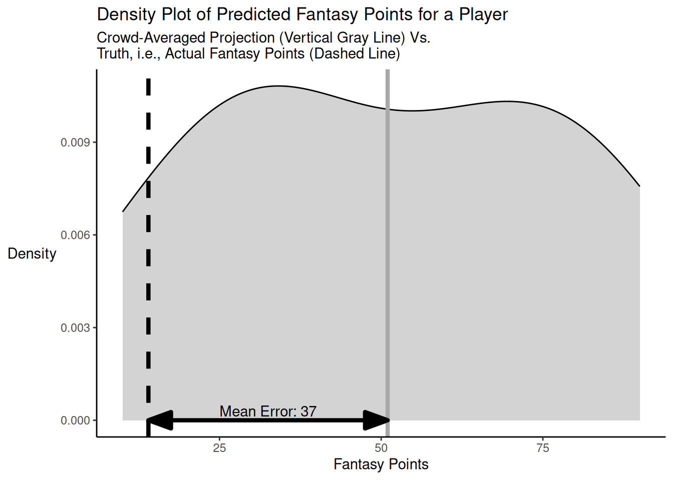
As demonstrated above, when the individual predictions bracket but are not centered on the truth and the bracketing rate is low (in this case, 25.00%), the crowd-averaged predictions (MAE/MdAE = 37) are more accurate than the accuracy of the typical individual forecaster (MAE = 38) in terms of mean absolute error, but they can still be less accurate—in terms of median absolute error—than the individual forecaster who is at the 50th percentile in accuracy (MdAE = 36).
Here is a code example of when the individual predictions do not bracket the truth for a player, and there are no strong outliers. The distribution of projected points versus truth is depicted in Figure 26.6.
Code
[1] -90 -80 -70 -60 -40 -30 -20 -10[1] 50Code
noBracketing1 <- petersenlab::wisdomOfCrowd(
  predicted = predictedValues,
  actual = actualValue
)

maeNoBracketing1_individual <- noBracketing1[which(row.names(noBracketing1) == "individual"), "MAE"]
maeNoBracketing1_crowd <- noBracketing1[which(row.names(noBracketing1) == "crowdAveraged"), "MAE"]

mdaeNoBracketing1_individual <- noBracketing1[which(row.names(noBracketing1) == "individual"), "MdAE"]
meNoBracketing1_crowd <- noBracketing1[which(row.names(noBracketing1) == "crowdAveraged"), "ME"]

ggplot2::ggplot(,
  mapping = aes(
    x = predictedValues)
) +
  geom_density(
    fill = "lightgray"
  ) +
  geom_vline(
    xintercept = mean(predictedValues),
    color = "darkgray",
    linewidth = 1.5) +
    geom_vline(
    xintercept = actualValue,
    linetype = "dashed",
    linewidth = 1.5
  ) +
  annotate(
    "segment",
    x = mean(predictedValues),
    xend = actualValue,
    y = 0,
    yend = 0,
    linewidth = 1.5,
    arrow = arrow(
      angle = 20,
      ends = "both",
      type = "closed")
  ) +
  annotate(
    "text",
    x = actualValue + (meNoBracketing1_crowd / 2),
    y = 0.0003,
    label = paste("Mean Error: ", meNoBracketing1_crowd, sep = ""),
    hjust = 0.5 # center-justify
  ) +
  labs(
    x = "Fantasy Points",
    y = "Density",
    title = "Density Plot of Predicted Fantasy Points for a Player",
    subtitle = "Crowd-Averaged Projection (Vertical Gray Line) Vs.\nTruth, i.e., Actual Fantasy Points (Dashed Line)"
  ) +
  theme_classic() +
  theme(axis.title.y = element_text(angle = 0, vjust = 0.5)) # horizontal y-axis title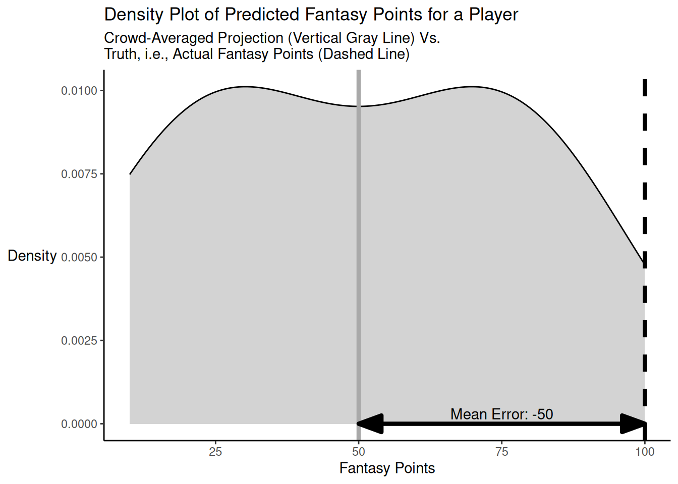
As demonstrated above, when the individual predictions do not bracket the truth (i.e., the bracketing rate is 0%) and there are no strong outliers, the crowd-averaged predictions (MAE/MdAE = 50) are as accurate as the accuracy of the typical individual forecaster (MAE = 50; MdAE = 50) in terms of mean absolute error and median absolute error.
Here is another code example of when the crowd-averaged predictions do not bracket the truth for a player and there is an outlier prediction that is far away from the truth. The distribution of projected points versus truth is depicted in Figure 26.7.
Code
[1] -100 -35 -33 -30 -20 -15 -10 -5[1] 69Code
noBracketing2 <- petersenlab::wisdomOfCrowd(
  predicted = predictedValues,
  actual = actualValue
)

maeNoBracketing2_individual <- noBracketing2[which(row.names(noBracketing2) == "individual"), "MAE"]
maeNoBracketing2_crowd <- noBracketing2[which(row.names(noBracketing2) == "crowdAveraged"), "MAE"]

mdaeNoBracketing2_individual <- noBracketing2[which(row.names(noBracketing2) == "individual"), "MdAE"]
meNoBracketing2_crowd <- noBracketing2[which(row.names(noBracketing2) == "crowdAveraged"), "ME"]

ggplot2::ggplot(,
  mapping = aes(
    x = predictedValues)
) +
  geom_density(
    fill = "lightgray"
  ) +
  geom_vline(
    xintercept = mean(predictedValues),
    color = "darkgray",
    linewidth = 1.5) +
    geom_vline(
    xintercept = actualValue,
    linetype = "dashed",
    linewidth = 1.5
  ) +
  annotate(
    "segment",
    x = mean(predictedValues),
    xend = actualValue,
    y = 0,
    yend = 0,
    linewidth = 1.5,
    arrow = arrow(
      angle = 20,
      ends = "both",
      type = "closed")
  ) +
  annotate(
    "text",
    x = actualValue + (meNoBracketing2_crowd / 2),
    y = 0.0015,
    label = paste("Mean Error: ", meNoBracketing2_crowd, sep = ""),
    hjust = 0.5 # center-justify
  ) +
  labs(
    x = "Fantasy Points",
    y = "Density",
    title = "Density Plot of Predicted Fantasy Points for a Player",
    subtitle = "Crowd-Averaged Projection (Vertical Gray Line) Vs.\nTruth, i.e., Actual Fantasy Points (Dashed Line)"
  ) +
  theme_classic() +
  theme(axis.title.y = element_text(angle = 0, vjust = 0.5)) # horizontal y-axis title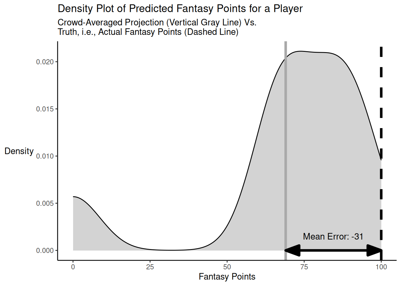
As demonstrated above, when the crowd-averaged predictions do not bracket the truth and there are one or more predictions that are far away from the truth, the crowd-averaged predictions (MAE/MdAE = 31) are as accurate as the accuracy of the typical individual forecaster (MAE = 31) in terms of mean absolute error, but they can be less accurate—in terms of median absolute error—than the individual forecaster who is at the 50th percentile in accuracy (MdAE = 25).
In conclusion, as demonstrated from these examples, when the crowd-averaged predictions are centered on the truth, the crowd-averaged predictions are perfectly accurate and are more accurate than the accuracy of the typical individual forecaster in terms of mean absolute error and of most individual forecasters in terms of median absolute error. When the crowd-averaged predictions bracket but are not centered on the truth, the crowd-averaged predictions are more accurate than the accuracy of the typical individual forecaster in terms of mean absolute error. If the bracketing rate is high and there are no strong outliers, the crowd-averaged predictions will also be more accurate—in terms of median absolute error—than most individual forecasters; however, if the bracketing rate is low or there are strong outliers, the crowd-averaged predictions can be less accurate than than most individual forecasters. Outliers could make the crowd-averaged prediction more or less accurate, depending on whether the outlying prediction is closer to or farther away from the truth, compared to the other predictions. When the crowd-averaged predictions do not bracket the truth, the crowd-averaged predictions are as accurate as the accuracy of the typical individual forecaster in terms of mean absolute error. When the crowd-averaged predictions do not bracket the truth and there are outliers, the crowd-averaged projections can be less accurate—in terms of median absolute error—than most individual forecasters (again, depending on whether the outlying prediction is closer to or farther away from the truth, compared to the other predictions).
In sum, going with crowd-averaged projections will always yield predictions that are as or more accurate (in terms of mean absolute error) than the (collective) accuracy of the individuals’ projections. However, the crowd-averaged projections may be less accurate than any individual projection, including the projection of the forecaster who is at the 50th percentile in accuracy. That is, if there is a low bracketing rate or inaccurate outliers, the crowd-averaged projections can be less accurate than most individual projections. In general, the higher the bracketing rate and the more closely that the projections are centered on the truth, the more accurate the crowd-averaged projections will be.
There may be multiple ways of handling outlier predictions. For instance, instead of computing a simple average of the predictions, one could calculate a weighted average that weights each prediction according to the historical accuracy of the prediction source. Alternatively, one could calculate the crowd-averaged prediction using an index of the center of a distribution that is less sensitive to outliers, such as a median or robust average such as the Hodges-Lehmann statistic (aka pseudomedian).
Even though some sources are more accurate than the average in a given year, they are not consistently more accurate than the average. Prediction involves a combination of luck and skill. In some years, a prediction will invariably do better than others, in part, based on luck. However, luck is unlikely to continue systematically into future years, so a source that got lucky in a given year is likely to regress to the mean in subsequent years. That is, determining the most accurate source in a given year, after the fact, is not necessarily the same as identifying the most skilled forecaster. It is easy to identify the most accurate source after the fact, but it is challenging to predict, in advance, who the best forecaster will be (Larrick et al., 2024). It requires a large sample of predictions to determine whether a given forecaster is reliably (i.e., consistently) more accurate than other forecasters and to identify the most accurate forecaster (Larrick et al., 2024). Thus, it can be challenging to know, in advance, who the most accurate forecasters will be. Because average projections are as or more accurate than the average forecaster’s prediction, averaging projections across all forecasters is superior to choosing individual forecasters when the forecasters are roughly similar in forecasting ability or when it is hard to distinguish their ability in advance (Larrick et al., 2024).
The relatively modest accuracy of the projections by so-called fantasy “experts” and of the average of their projections could occur for a number of reasons. One possibility is that the level of expertise of the “expert” forecasters in terms of being able to provide accurate forecasts is not strong. That is, because football performance and injuries are so challenging to predict, individual forecasters’ projections may not be particularly close to the truth.
A second possibility is that the bracketing rate of the predictions is not particularly high (Mannes et al., 2014). Even if the individual forecasters’ projections are not close to the truth, if ~50% of them overestimate the truth and the other 50% of the underestimate the truth, the average will more closely approximate the truth. However, if all forecasters overestimate the truth for a given player, averaging the projections will not necessarily lead to more accurate projections.
A third possibility is that the forecasts of the different experts are not independent.
Each of these possibilities is likely true to some degree. First, individuals’ predictions are unlikely to be highly accurate consistently. Second, there are many players who are systematically overpredicted (e.g., due to their injury) or underpredicted (e.g., due to their becoming the starter after a teammate becomes injured, is traded, etc.)—an example of overextremity miscalibration. In general, it is likely for players who are projected to score more points to be overpredicted and for players who are projected to score fewer points to be underpredicted, as described in Section 17.12. Third, the experts may interact and discuss with one another. Interaction and discussion among experts may lead them to follow the herd and conform their projections to what each other predict. This has been termed “informational influence” and may reflect the anchoring and adjustment heuristic (Larrick et al., 2024). In any case, they are able to see each other’s projections and make change their projections, accordingly.
26.4.2 Seasonal Projections
Code
seasonalIndividualSources <- projectionsWithActuals_seasonal |>
  filter(!is.na(raw_points)) |>
  filter(!is.na(fantasyPoints)) |>
  group_by(player_id, season) |>
  filter(n() >= 2) |> # at least 2 projections
  summarise(
    numProjections = n(),
    type = "individual",
    petersenlab::wisdomOfCrowd(
      predicted = raw_points,
      actual = unique(fantasyPoints),
      dropUndefined = TRUE
      )[1,],
    .groups = "drop"
  )

seasonalCrowd <- projectionsWithActuals_seasonal |>
  filter(!is.na(raw_points)) |>
  filter(!is.na(fantasyPoints)) |>
  group_by(player_id, season) |>
  filter(n() >= 2) |> # at least 2 projections
  summarise(
    numProjections = n(),
    type = "crowd",
    petersenlab::wisdomOfCrowd(
      predicted = raw_points,
      actual = unique(fantasyPoints),
      dropUndefined = TRUE
      )[2,],
    .groups = "drop"
  )

seasonalIndividualSourcesAndCrowd <- bind_rows(
  seasonalIndividualSources,
  seasonalCrowd
)

seasonalIndividualSources <- seasonalIndividualSources |>
  left_join(
    player_stats_seasonal,
    by = c("player_id", "season")
  )

seasonalCrowd <- seasonalCrowd |>
  left_join(
    player_stats_seasonal,
    by = c("player_id", "season")
  )

seasonalIndividualSourcesAndCrowd <- seasonalIndividualSourcesAndCrowd |>
  left_join(
    player_stats_seasonal,
    by = c("player_id", "season")
  )
Code
Code
ggplot2::ggplot(
  data = seasonalIndividualSources |>
    filter(position_group %in% c("QB","RB","WR","TE")),
  mapping = aes(
    x = bracketingRate)
) +
  geom_histogram(
    color = "#000000",
    fill = "#0099F8"
  ) +
  labs(
    x = "Bracketing Rate",
    y = "Count",
    title = "Histogram of Bracketing Rate (Seasonal Projections)"
  ) +
  theme_classic() +
  theme(axis.title.y = element_text(angle = 0, vjust = 0.5))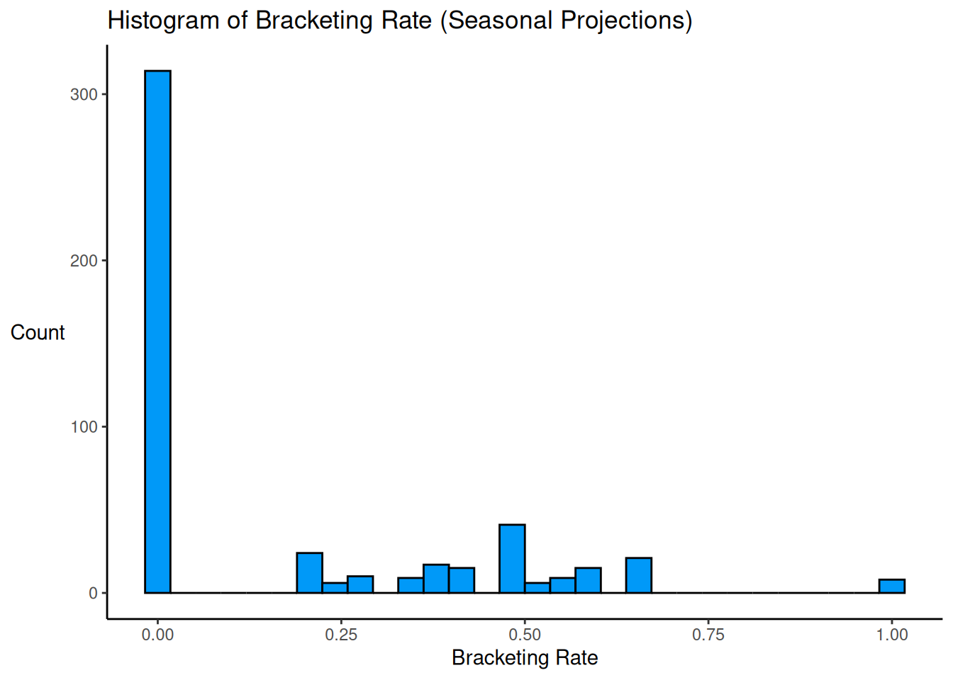
Below is the proportion of players whose bracketing rate was zero:
Code
A high proportion (68%) of players’ forecasts did not bracket the truth.
26.4.3 Weekly Projections
Code
weeklyIndividualSources <- projectionsWithActuals_weekly |>
  filter(!is.na(raw_points)) |>
  filter(!is.na(fantasyPoints)) |>
  group_by(player_id, season, week) |>
  filter(n() >= 2) |> # at least 2 projections
  summarise(
    numProjections = n(),
    type = "individual",
    petersenlab::wisdomOfCrowd(
      predicted = raw_points,
      actual = unique(fantasyPoints),
      dropUndefined = TRUE
      )[1,],
    .groups = "drop"
  )

weeklyCrowd <- projectionsWithActuals_weekly |>
  filter(!is.na(raw_points)) |>
  filter(!is.na(fantasyPoints)) |>
  group_by(player_id, season, week) |>
  filter(n() >= 2) |> # at least 2 projections
  summarise(
    numProjections = n(),
    type = "crowd",
    petersenlab::wisdomOfCrowd(
      predicted = raw_points,
      actual = unique(fantasyPoints), # [1] error w/o [1] because have more than one unique value for a given player-season-week
      dropUndefined = TRUE
      )[2,],
    .groups = "drop"
  )

weeklyIndividualSourcesAndCrowd <- bind_rows(
  weeklyIndividualSources,
  weeklyCrowd
)

weeklyIndividualSources <- weeklyIndividualSources |>
  left_join(
    player_stats_weekly,
    by = c("player_id", "season", "week")
  )

weeklyCrowd <- weeklyCrowd |>
  left_join(
    player_stats_weekly,
    by = c("player_id", "season", "week")
  )

weeklyIndividualSourcesAndCrowd <- weeklyIndividualSourcesAndCrowd |>
  left_join(
    player_stats_weekly,
    by = c("player_id", "season", "week")
  )
Code
Code
ggplot2::ggplot(
  data = weeklyIndividualSources |>
    filter(position_group %in% c("QB","RB","WR","TE")),
  mapping = aes(
    x = bracketingRate)
) +
  geom_histogram(
    color = "#000000",
    fill = "#0099F8"
  ) +
  labs(
    x = "Bracketing Rate",
    y = "Count",
    title = "Histogram of Bracketing Rate (Weekly Projections)"
  ) +
  theme_classic() +
  theme(axis.title.y = element_text(angle = 0, vjust = 0.5))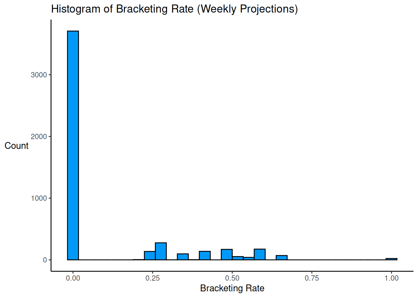
Below is the proportion of players whose bracketing rate was zero:
Code
A high proportion (77%) of players’ forecasts did not bracket the truth.
26.5 How Well Do People Incorporate Advice From Others?
An important question is how well people incorporate advice from others. In the context of fantasy football, advice might be sources of projections. In general, evidence from social psychology suggests that people tend to underweight how much weight they give to advice from others relative to their own opinions, a phenomenon called egocentric discounting (Larrick et al., 2024; Rader et al., 2017). People tend to weight others’ advice around 30% in terms of the proportion of a shift a person makes toward another person’s perspective, though this depends on the perceived accuracy of the advisor. Moreover, people frequently ignores others’ advice entirely. In general, people make use of crowds too little—they put too much weight on their own prediction and not enough weight on others’ predictions whose diversity can be leveraged for error cancellation (Larrick et al., 2024). This could reflect, in part, the incorrect assumption that the average judgment is no more accurate than the average judge (Larrick et al., 2024).
26.6 Strategies for Managing Risk and Uncertainty
Sports analyst Tanney (2021) encourages people to consider framing your decisions as bets, to use a probabilistic mindset (rather than a deterministic mindset). Even if something is perceived as likely to occur with 100% certainty, it is not guaranteed that such an event will occur. Other things can and do happen, and overconfidence can get in the way of effective decision-making.
A key goal is to identify decisions that provide a net advantage in expected value. Although there is considerable variability and the outcome is not guaranteed, small advantages can yield considerable gains in the long run (Tanney, 2021); however, one must be able to survive the costs of losses to obtain enough long-term trials. So, do not bet more than you are willing to lose.
26.7 Risk Management Principles from Cognitive Psychology
26.8 Sports Betting/Gambling
The National Football League (NFL) used to be adamantly against sports gambling. They wanted to protect the integrity of the game. They felt that sports gambling might lead to match fixing, point shaving, and other forms of corruption that would undermine the legitimacy of competition in the game. Match fixing occurs when players, referees, coaches, or others conspire to manipulate the outcome of the game. Point shaving involves manipulating the score—commonly by a player intentionally underperforming (even if it does not lead to “throwing the game” and causing the team to lose). Match fixing and point shaving can occur for a variety of reasons, but a common reason is to ensure that particular gamblers win their bet. Another reason the NFL was against sports betting was that, prior to the U.S. Supreme Court overturning the Professional and Amateur Sports Protection Act (PASPA) in 2018, there were legal restrictions on gambling that prevented sports betting in many parts of the country.
However, after the legalization of sports betting following the overturning of PASPA in 2018, the NFL has changed their tune and are now strongly in favor of sports betting. The rise of legal sports betting has created massive revenue streams for the NFL through partnerships, sponsorships, and advertising deals with sportsbooks.
There is substantial overconfidence (in particular overestimation of one’s actual performance) in sports betting/gambling. A study (archived at https://perma.cc/X2AW-SUBZ) of frequent sports bettors found that they tended to predict that they would gain 0.3 cents for every dollar wagered, but in fact lost 7.5 cents for every dollar wagered (Brown et al., 2025). Overconfidence was greatest among those who frequently wagered multi-leg bets (parlays), losing ~25 cents for every dollar wagered (Brown et al., 2025).
People may make a sports bet because they believe strongly in their predicted outcome and that they “cannot be wrong”. However, the initial Vegas lines represent the aggregation of a massive amount of information (by professional oddsmakers), including team power rankings, injuries, weather, home/away, coaching, matchups, historical betting behavior, advanced statistics, and proprietary algorithms. Leading up to the game, the Vegas lines are adjusted to balance the total money on each side of the bet (so that the sportsbook can be ensured it makes money). In this way, the Vegas lines are based on the bets of many, many people and many dollars and reflect market wisdom. That is, by making a sports bet, you are implicitly claiming that you have information, insight, or a model that makes you better than the market consensus at predicting the outcome—even though half of the dollars bet will lose. Betting markets, similar to the stock market (as described in Section 20.3.1), are often highly efficient and beating them consistently is extremely challenging. Moreover, people tend to show confirmation bias, such that they tend to remember their predictive successes and to forget their failures. So, when they get a bet correct, they may be more likely to bet again in the future, especially because sports betting involves intermittent reinforcement (in particular, variable ratio reinforcement), which can make it highly addictive.
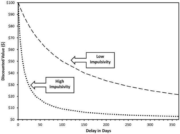
However, not all people are equally prone to gambling addiction. One of the most robust risk factors of gambling addiction is a steep delay discounting curve (Amlung et al., 2017; Weinsztok et al., 2021). The delay discounting curve can be generated from asking respondents a series of hypothetical choices, such as: 1) Would you prefer $10 now or $15 in 1 hour? 2) Would you prefer $10 now or $20 tomorrow? 3) Would you prefer $10 now or $50 in one month? Based on these questions, one can estimate how much a respondent’s valuation of a reward (in this case, money) decreases with the passage of time. An example of delay discounting curves of two people is in Figure 26.10. Some individuals have a shallow delay discounting curve and will prefer more money even if they have to wait, a form of delayed gratification. Other individuals have a steep delay discounting curve and will prefer obtaining the money now, even if that means gaining less money in the long run, a form of impulsivity. In particular, individuals who have a steep delay discounting curve are most likely to develop gambling addictions, possibly because they are more sensitive to immediate rewards and are less driven by long-term consequences.
26.8.1 Reinforcement
Reinforcement involves a (typically appetitive) stimulus that increases the frequency of a behavior. For instance, reinforcers could include things like food, praise, attention, money, etc. Thus, sports gambling can provide reinforcement through the receipt of money.
26.8.1.1 Continuous Reinforcement
In general, when you want to train a new behavior, continuous reinforcement is the fastest way to do so. Continuous reinforcement means rewarding the behavior each time that it occurs. For instance, a parent might use continuous reinforcement to train their child to put their toys away—the parent may praise them or give them physical affection each time they put their toys away. However, continuous reinforcement is susceptible to extinction. Extinction means cessation of the target behavior (putting the toys away, in this example). That is, for a previously continuously reinforced behavior, if the behavior stops being rewarded, the person is less likely to continue the behavior. Thus, to make a behavior less susceptible to extinction, intermittent reinforcement may be used.
26.8.1.2 Intermittent Reinforcement
Intermittent reinforcement (also called partial reinforcement) means rewarding the behavior sometimes but not everytime. There are various approaches to intermittent reinforcement, called schedules of reinforcement. The four primary reinforcement schedules are: fixed interval, fixed ratio, variable interval, and variable ratio. The reinforcement schedules are depicted in Figure 26.11, as adapted from Spielman et al. (2020).
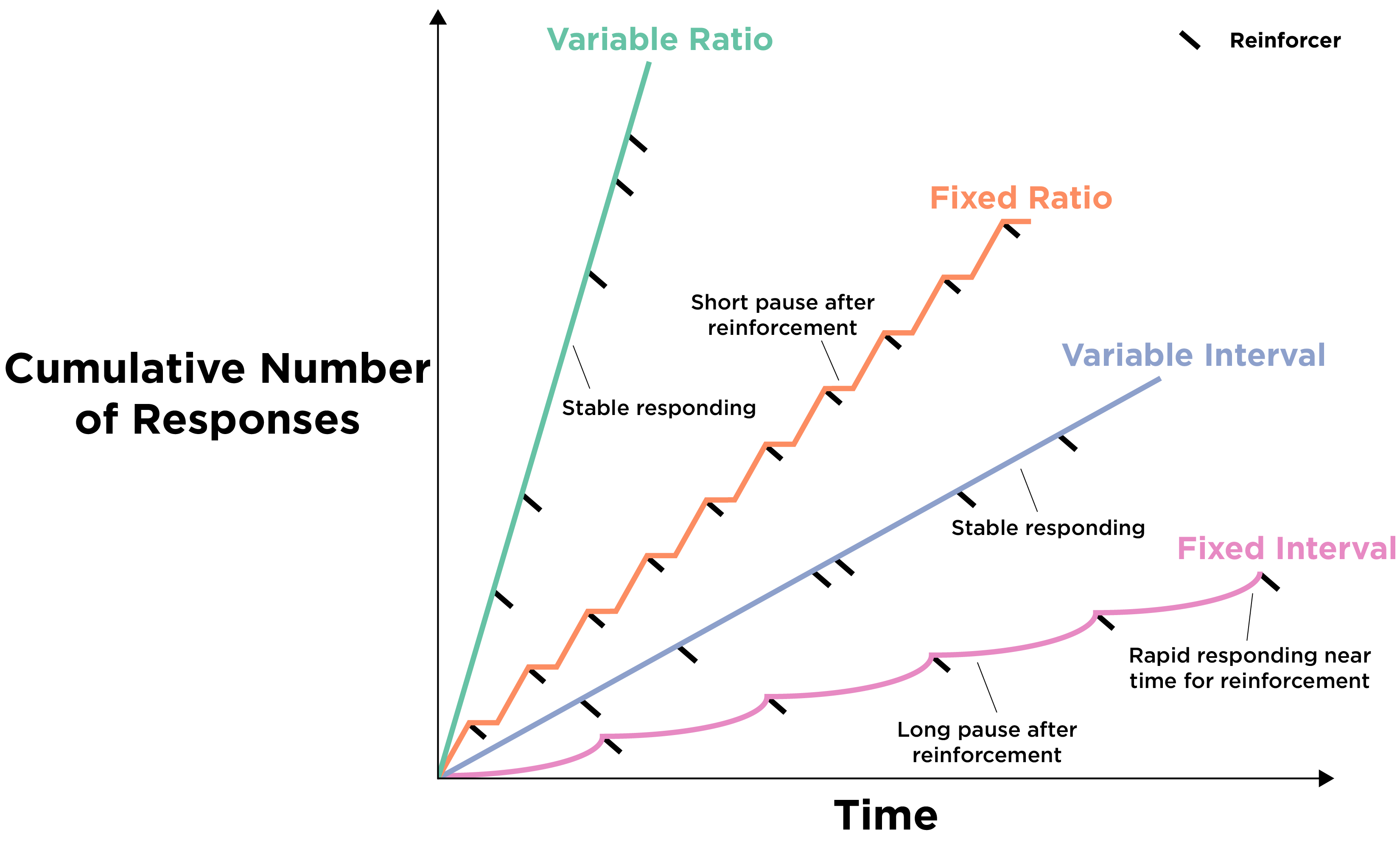
A fixed interval reinforcement schedule occurs when the person is rewarded after a set amount of time. For instance, if the reward becomes available every 30 minutes, the person receives the reward the first time they engage in the behavior after the reward becomes available. As an example, consider a surgery patient who can receive a painkiller after pressing a button, but only up to once per hour.
A variable interval reinforcement schedule occurs when the person is rewarded after a varying (and unpredictable) amount of time. As an example, consider a restaurant manager who is paid a bonus if the food inspector, who comes at unpredictable times, gives the restaurant a good rating.
A fixed ratio reinforcement schedule occurs when the person is rewarded after a set number of responses. As an example, consider a coffee shop that offers a free coffee after every 10 purchases that a person makes.
A variable ratio reinforcement schedule occurs when the person is rewarded after a varying (and unpredictable) number of responses. As an example, consider a slot machine that provides a large monetary reward (paired with the machine lighting up and bells going off) after a varying number of attempts. Many forms of gambling involve variable ratio reinforcement.
The variable ratio reinforcement schedule is the least susceptible to extinction. People can go without reinforcement many times and may still continue to gamble out of the hope for a large reward on the next attempt. The low susceptibility of variable ratio reinforcement to extinction is, in part, why gambling (which often involves variable ratio reinforcement) can be highly addictive despite people’s tendency to lose money gambling.
26.8.2 Is Fantasy Football a Game of Luck or Skill?
The question of whether fantasy football is a game of chance or skill is important because such considerations help determine whether betting on one’s performance is considered gambling, which might be illegal or regulated in many jurisdictions. Fantasy football (and sports betting, more generally) is not 100% luck. Skill can be involved in identifying undervalued assets—whether in terms of stocks in the stock market or professional football players, where inside information can be especially valuable (and thus illegal to profit from). To evaluate the percentage of variability in fantasy football that is attributable to luck versus skill, Getty et al. (2018) evaluated the extent to which one’s performance in the first half of the season was correlated with one’s performance in the second half of the season, under the assumption that underlying skill would lead to persistence of performance across time. The authors examined FanDuel daily fantasy sports (DFS) leagues, which allow the user to set an entirely new lineup each week from all players, based on salary constraints (so a user cannot just select the best player at every position). The authors estimated that ~55% of the variability in fantasy football performance across time was due to skill and 45% was due to luck (Getty et al., 2018). Thus, performance in fantasy football is around half and half luck versus skill.
Because fantasy football is not 100% luck, it is not the same as a slot machine. However, there are still unpredictable elements (e.g., injuries), and there is considerable luck involved. As a result, sports betting and gambling on fantasy football still involve components of variable ratio reinforcement that lend them to being potentially highly addictive despite people’s tendency to lose money.
26.9 Suggestions
Based on the above discussion, here are some suggestions for decision making in the context of uncertainty:
- Seek advice from diverse perspectives and incorporate it into your decision making.
- Get opinions from others before you state your perspective and before the various sources of advice discuss with each other, to ensure independence of advice.
- As noted by Kahneman (2011), “before an issue is discussed, all members of the committee should be asked to write a very brief summary of their position… The standard practice of open discussion gives too much weight to the opinions of those who speak early and assertively, causing others to line up behind them.” (p. 85).
- If some sources of advice (or projections) are clearly more skilled and accurate than others, you can average this “select” crowd of projections or give them greater weight in a weighted average.
- If it is unclear whether or which sources are reliably more accurate than others, using a simple average across all sources (i.e., crowd-averaged projections) can be a useful approach that is as accurate as—if not more accurate than—the average individual forecaster.
- Incorporate at least 5–10 sources of projections. Use a weighted or robust average to account for outlier projections.
- Do not bet on fantasy football (or anything else for that matter) unless you are willing to lose the money. Sports bettors tend to be overconfident; on average, they lose 7.5 cents for every dollar wagered (Brown et al., 2025). If you are going to bet, only bet a small portion of your money and never more than you are willing to lose. And do not make multi-leg bets (parlays); people lose on average 25 cents for every dollar wagered on parlays (Brown et al., 2025).
26.10 Conclusion
The wisdom of the crowd is the idea that the average of the predictions of many people is often more accurate than the prediction of individual experts. When at least some of the projections bracket—i.e., fall on opposite sides of—the truth, averaged predictions are more accurate than the average individual forecaster—in terms of mean absolute error (MAE). Crowd-averaged projections tend to be most accurate when the crowd consists of individuals who hold expertise in the domain such that they will make predictions that fall close to the truth, there is relatively low variability in the expertise of the individual forecasters in terms of their ability to make accurate forecasts, there is cognitive diversity among the forecasters, the projections are made independently—i.e., the forecasters are not aware of others’ forecasts and do not discuss or interact with the other forecasters, the bracketing rate is high, and there are at least 5–10 sources of projections. In the case of fantasy football, however, a high proportion of players’ forecasts do not bracket the truth, suggesting that the so-called experts are not accurate in predicting players’ future fantasy performance. Nevertheless, going with the crowd-averaged projections tends to be more accurate than relying on an individual projection source. Performance in fantasy football is around half and half luck versus skill. Sports betting and gambling on fantasy football involve components of variable ratio reinforcement that lend them to being potentially highly addictive.
26.11 Session Info
R version 4.6.1 (2026-06-24)
Platform: x86_64-pc-linux-gnu
Running under: Ubuntu 24.04.4 LTS

Matrix products: default
BLAS:   /usr/lib/x86_64-linux-gnu/openblas-pthread/libblas.so.3
LAPACK: /usr/lib/x86_64-linux-gnu/openblas-pthread/libopenblasp-r0.3.26.so;  LAPACK version 3.12.0

locale:
 [1] LC_CTYPE=C.UTF-8       LC_NUMERIC=C           LC_TIME=C.UTF-8
 [4] LC_COLLATE=C.UTF-8     LC_MONETARY=C.UTF-8    LC_MESSAGES=C.UTF-8
 [7] LC_PAPER=C.UTF-8       LC_NAME=C              LC_ADDRESS=C
[10] LC_TELEPHONE=C         LC_MEASUREMENT=C.UTF-8 LC_IDENTIFICATION=C

time zone: UTC
tzcode source: system (glibc)

attached base packages:
[1] stats     graphics  grDevices utils     datasets  methods   base

other attached packages:
 [1] lubridate_1.9.5   forcats_1.0.1     stringr_1.6.0     dplyr_1.2.1
 [5] purrr_1.2.2       readr_2.2.0       tidyr_1.3.2       tibble_3.3.1
 [9] ggplot2_4.0.3     tidyverse_2.0.0   petersenlab_1.2.3

loaded via a namespace (and not attached):
 [1] tidyselect_1.2.1   psych_2.6.5        viridisLite_0.4.3  farver_2.1.2
 [5] S7_0.2.2           fastmap_1.2.0      digest_0.6.39      rpart_4.1.27
 [9] timechange_0.4.0   lifecycle_1.0.5    cluster_2.1.8.2    magrittr_2.0.5
[13] compiler_4.6.1     rlang_1.3.0        Hmisc_5.2-6        tools_4.6.1
[17] yaml_2.3.12        data.table_1.18.4  knitr_1.51         labeling_0.4.3
[21] htmlwidgets_1.6.4  mnormt_2.1.2       plyr_1.8.9         RColorBrewer_1.1-3
[25] foreign_0.8-91     withr_3.0.3        nnet_7.3-20        grid_4.6.1
[29] stats4_4.6.1       lavaan_0.7-2       xtable_1.8-8       colorspace_2.1-3
[33] scales_1.4.0       MASS_7.3-65        cli_3.6.6          mvtnorm_1.4-2
[37] rmarkdown_2.31     reformulas_0.4.4   generics_0.1.4     otel_0.2.0
[41] rstudioapi_0.19.0  reshape2_1.4.5     tzdb_0.5.0         minqa_1.2.8
[45] DBI_1.3.0          splines_4.6.1      parallel_4.6.1     base64enc_0.1-6
[49] mitools_2.4        vctrs_0.7.3        boot_1.3-32        Matrix_1.7-5
[53] jsonlite_2.0.0     hms_1.1.4          Formula_1.2-5      htmlTable_2.5.0
[57] glue_1.8.1         nloptr_2.2.1       stringi_1.8.7      gtable_0.3.6
[61] quadprog_1.5-8     lme4_2.0-6         pillar_1.11.1      htmltools_0.5.9
[65] R6_2.6.1           Rdpack_2.6.6       mix_1.0-13         evaluate_1.0.5
[69] pbivnorm_0.6.0     lattice_0.22-9     rbibutils_2.4.1    backports_1.5.1
[73] Rcpp_1.1.2         gridExtra_2.3.1    nlme_3.1-169       checkmate_2.3.4
[77] xfun_0.60          pkgconfig_2.0.3