I want your feedback to make the book better for you and other readers. If you find typos, errors, or places where the text may be improved, please let me know. The best ways to provide feedback are by GitHub or hypothes.is annotations.
You can leave a comment at the bottom of the page/chapter, or open an issue or submit a pull request on GitHub: https://github.com/isaactpetersen/Fantasy-Football-Analytics-Textbook
Alternatively, you can leave an annotation using hypothes.is.
To add an annotation, select some text and then click the
symbol on the pop-up menu.
To see the annotations of others, click the
symbol in the upper right-hand corner of the page.
13 Causal Inference
This chapter provides an overview of principles of causal inference and causal diagrams.
13.1 Getting Started
13.1.1 Load Packages
13.2 Causation
A causal effect is the difference in an outcome that is directly attributable to different levels or values of an input variable. It reflects the difference in the outcome that would be observed for the same unit under two or more different levels of the input variable, holding all other relevant factors constant. For instance, for a given player, the extent to which consumption of sports drink influences their performance reflects the difference between how well the player would perform if they consume sports drink compared to how well they would perform if they do not consume sports drink.
13.3 Correlation Does Not Imply Causation
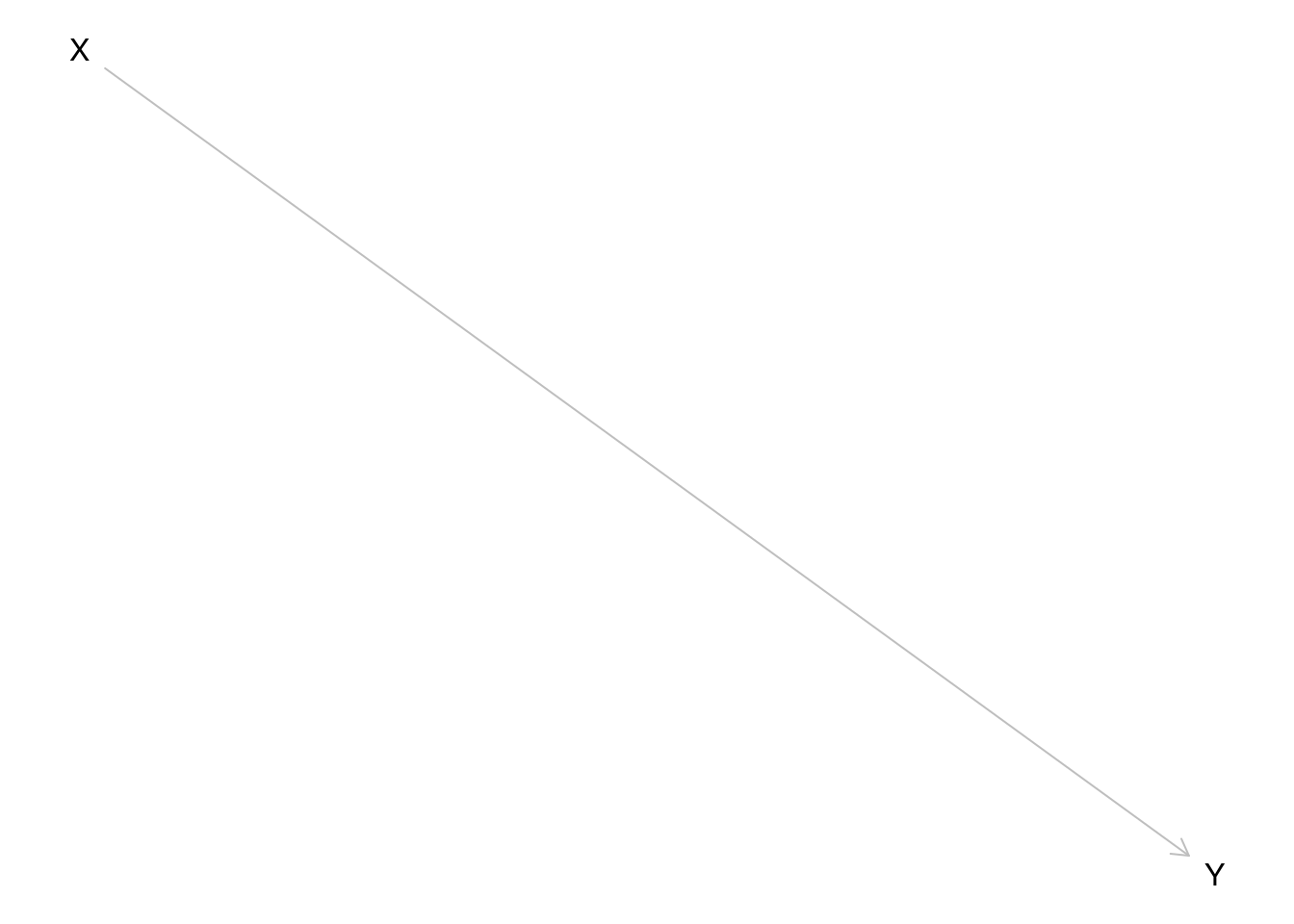
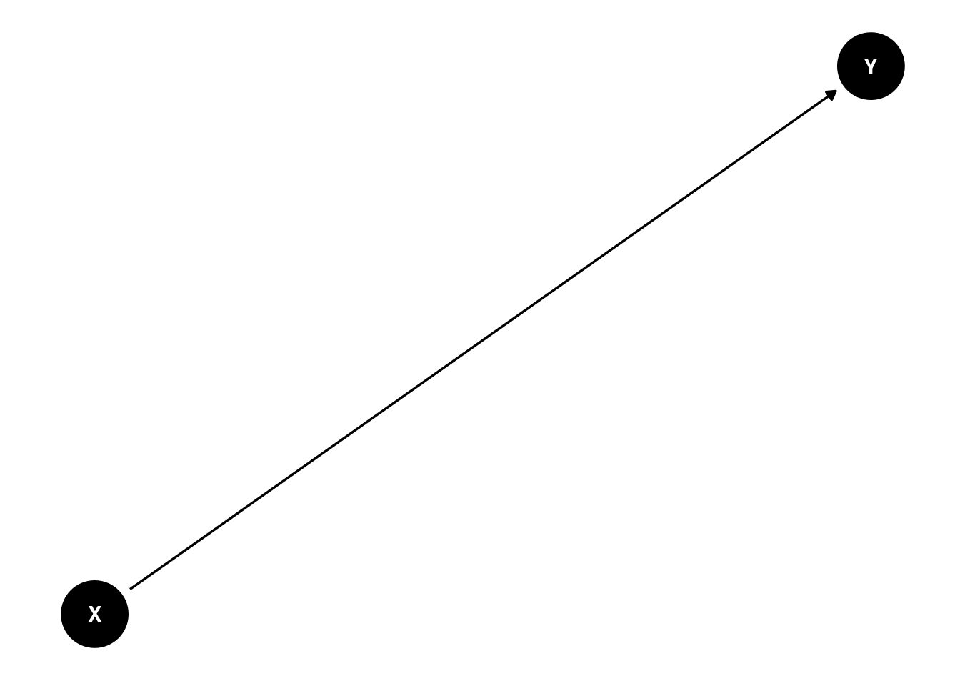
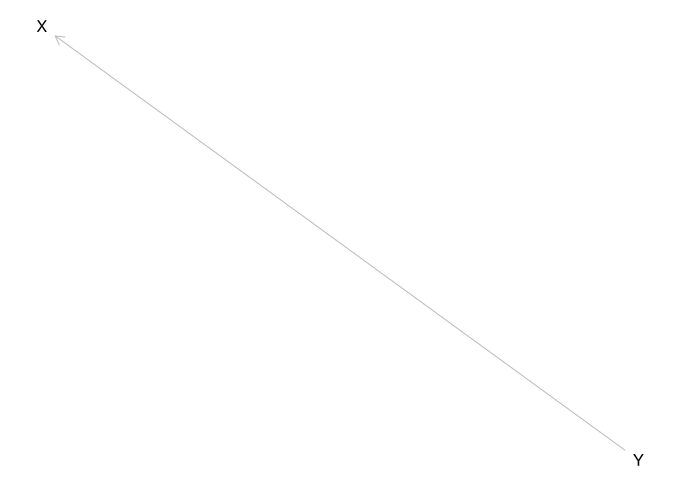
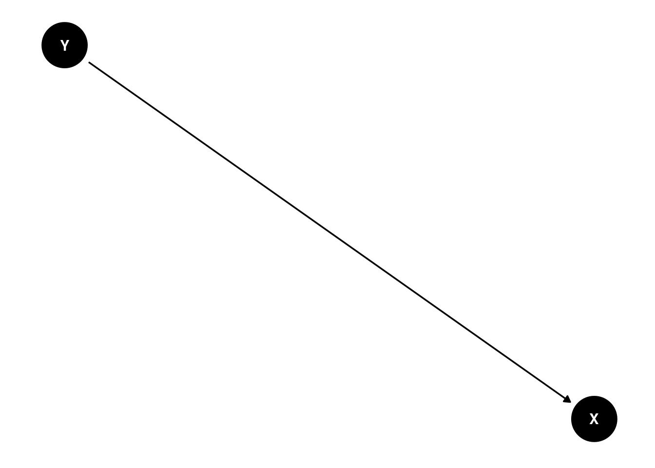
As described in Section 8.5.2.1, there are several reasons why two variables, X and Y, might be correlated:
-
XcausesY -
YcausesX -
XandYare bidirectional:XcausesYandYcausesX - a third variable (i.e., confound),
Z, influences bothXandY - the association between
XandYis spurious (noncausal and due to random chance)
13.4 Criteria for Causality
How do we know whether two processes are causally related? There are three criteria for establishing causality (Shadish et al., 2002):
- The cause (e.g., the independent or predictor variable) temporally precedes the effect (i.e., the dependent or outcome variable).
- The cause is related to (i.e., associated with) the effect.
- There are no other alternative explanations for the effect apart from the cause.
The first criterion for establishing causality involves temporal precedence. In order for a cause to influence an effect, the cause must occur before the effect. For instance, if sports drink consumption influences player performance, the sports drink consumption (that is presumed to influence performance) must occur prior to the performance improvement. Establishing the first criterion eliminates the possibility that the association between the purported cause and effect reflects reverse causation. Reverse causation occurs when the purported effect is actually the cause of the purported cause, rather than the other way around. For instance, if sports drink consumption occurs only once, and it occurs only before and not after performance, then we have ruled out the possibility of reverse causation (i.e., that better performance causes players to consume sports drink). To help establish the first criterion, experiments and longitudinal designs are useful.
The second criterion involves association. The purported cause must be associated with the purported effect. Nevertheless, as the maxim goes, “correlation does not imply causation.” Just because two variables are correlated does not necessarily mean that they are causally related. However, correlation is useful because causality requires that the two processes be correlated. That is, correlation is a necessary but insufficient condition for causality. For instance, if sports drink consumption (directly) influences player performance, sports drink consumption must be associated with performance improvement.
Even though a cause and its (direct) effect must be related (i.e., covary), it is not necessarily the case—for multiple reasons—that you would detect an association between a cause and an effect. First, the association may be nonlinear. If you are trying to detect an association using Pearson correlation, which assumes a linear association, the (nonlinear) association may go undetected. Second, from a cause to a downstream effect, multiple causal pathways with opposing signs may cancel out in the aggregate. A cause may have both beneficial and harmful effects on the outcome, and the mediating mechanisms can “cancel each other out”. For instance, the cause may help via mechanism A, but may hurt via mechanism B. That is, consider if the cause, X, influences the effect, Y, via two mechanisms, A and B (i.e., mediation)—and that X has a positive influence on A (i.e., the association is positive), whereas X has a negative influence on B (i.e., the association is negative). In that case, the effects of the mediating mechanisms can cancel each other out, leaving no observable bivariate association between X and Y. Alternatively, a null association between X and Y can also arise if a confound influences both X and Y in an opposing direction to the effect of X on Y. For example, X may (positively) influence Y via mediator A, whereas B is a confound with a negative effect on Y. In that case, the positive effect through A and the negative effect from B can cancel, so no association may be observed unless the confound is controlled for; failing to control for the confound is an example of omitted variable bias. So, a null association does not imply no causal effect. Wrongly inferring that a causal effect of one variable on another is not causal is an example of conclusion invalidity arising from a failure to account for the underlying causal mechanisms of X on Y.
The third criterion involves ruling out alternative reasons why the purported cause and effect may be related. As noted in Section 13.3, there are five reasons why X may be correlated with Y. If we meet the first criterion of causality, we have removed the possibility that Y causes X (i.e., reverse causality). To meet the third criterion of causality, we need to remove the possibility that the association reflects a third variable (confound) that influences both the cause and effect, and we need to remove the possibility that the association is spurious—the possibility that the association between the purported cause and effect is due to random chance.
There are multiple approaches to meeting the third criterion of causality, such as by use of experiments, longitudinal designs, control variables, within-subject designs, and genetically informed designs, as described in Section 13.5.
In general, to meet the third criterion of causality, one must consider the counterfactual—what would have happened “counter to the fact”. A counterfactual is what would have happened in the hypothetical scenario that the cause did not occur [i.e., what would have happened in the absence of the cause; Shadish et al. (2002)]. When engaging in causal inference, it is important to consider what would have happened if the hypothetical cause had actually not occurred. It is like an alternate universe where the cause did not happen. For instance, consider that we conduct an experiment to randomly assign some players to consume a sports drink before a game and other players to drink only water. In this case, our treatment/intervention group is the group of players that consumed a sports drink. The control group is the group players that drank only water. Now, consider that the players in the treatment group outperform the players in the control group in their football game. In such a study, we observe what did happen when players received a treatment. The counterfactual is knowledge of what would have happened to those same players if they simultaneously had not received treatment (Shadish et al., 2002). The true causal effect, then, is the difference between what did happen and what would have happened. However, we cannot observe a counterfactual. This is the fundamental problem of causal inference—we only observe one potential world/outcome/universe. That is, we do not know for sure what would have happened to the players who received treatment if those same players had actually not received treatment. We have a control group, but the control group does not have the same players as the intervention group, and it is impossible for a person to simultaneously receive and not receive treatment. Thus, an individual causal effect cannot typically be identified (D’Onofrio et al., 2020).
So, our goal in working toward causal inference as scientists is to create reasonable approximations to this impossible counterfactual (Shadish et al., 2002). For instance, if using a between-subject design, we want the two groups to be equivalent in every possible way except whether or not they receive the treatment, so we might stratify each group to be equivalent in terms of age, weight, position, experience, skill, etc. Or, we might test the same people using an A-B-A-B within-subject design. In an A-B-A-B within-subject design, players receive no treatment at baseline (timepoint 1: game 1), receive the treatment at timepoint 2 (game 2), receive no treatment at timepoint 3 (game 3), and receive the treatment at timepoint 4 (game 4). Neither of these approximations is a true counterfactual. In the between-subject design, the players differ between the two groups, so we cannot know how the individuals who received the treatment would have performed if they had actually not received the treatment. In the A-B-A-B within-subject design, all players receive the same sequence of alternating conditions—no treatment, treatment, no treatment, treatment—across four timepoints. Although the A-B-A-B within-subject design keeps participants constant, the specific occasion of measurement may differ from participant to participant (thus introducing time or context of measurement as a potential confound), and there can be carryover effects from one condition to the next. For instance, consuming sports drinks before game 2 might also help the player be better hydrated in general, including for subsequent games. Thus, we cannot know how a player would have performed in game 1 with treatment or in game 2 without treatment, and so on. Nevertheless, it is important to be aware of the counterfactual and to engage in counterfactual reasoning to consider what would have happened if the supposed cause had not occurred. Considering the counterfactual is important for designing closer approximations to the counterfactual in studies for stronger research designs and stronger causal inference.
13.5 Approaches for Causal Inference
Broadly, approaches for causal inference encompass 1) analysis approaches that account for measured factors and 2) designs that account for unmeasured factors (D’Onofrio et al., 2020).
13.5.1 Experimental Designs
As described in Section 8.5.1, experimental designs are designs in which participants are randomly assigned to one or more levels of the independent variable to observe its effects on the dependent variable. Experimental designs provide the strongest tests of causality because they can rule out reverse causation and third variables. For instance, by manipulating sports drink consumption before the player performs, they can eliminate the possibility that reverse causation explains the effect of the independent variable on the dependent variable. Second, through randomly assigning players to consume or not consume sports drink, this holds everything else constant (so long as the groups are evenly distributed according to other factors, such as their age, weight, etc.) and thus removes the possibility that third variable confounds explain the effect of the independent variable on the dependent variable. However, not everything is able to, or ethical to, be manipulated. In addition, as described in Section 8.6.3, experimental designs tend to have lower capacity for external validity than correlational designs—that is, compared to findings from correlational designs, the findings from experimental designs tend to have lower capacity to be consistent with how things play out in the real world.
13.5.2 Quasi-Experimental Designs
Although experimental designs provide the strongest tests of causality, many times they are impossible, unethical, or impractical to conduct. For instance, it would likely not be practical to randomly assign National Football League (NFL) players to either consume or not consume sports drink before their games. Players have their pregame rituals and routines and many would likely not agree to participate in such a study. Moreover, as described in Section 8.6.3, experimental designs tend to be lower in external validity and thus their findings may not always generalize to how things occur in the real world. In addition, experimental designs commonly have sample sizes that are too small to study rare-but-serious outcomes (D’Onofrio et al., 2020). Thus, we often rely on (and need!) quasi-experimental designs such as natural experiments and observational/correlational designs.
We cannot directly test or establish causality from a non-experimental research design. Nevertheless, we can leverage various analysis approaches and design features that, in combination with other studies using different research methods, collectively strengthen our ability to make causal inferences. For instance, there are are no experiments in humans showing that smoking causes cancer—randomly assigning people to smoke or not smoke would not be ethical. The causal inference that smoking causes cancer was derived from a combination of experimental studies in rodents and observational studies in humans. To the extent that findings across designs that have different threats to research design validity show similar results in terms of the association between the predictor variable and the outcome variable, the case for causality is strengthened (D’Onofrio et al., 2020).
13.5.2.1 Longitudinal Designs
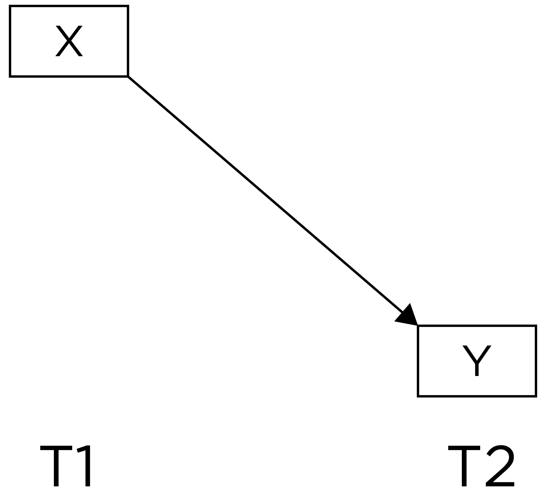
Research designs can be compared in terms of their internal validity—the extent to which we can be confident about causal inferences. A cross-sectional association is depicted in Figure 13.1:
For instance, we might observe that sports drink consumptions is concurrently associated with better player performance. Among observational/correlational research designs, cross-sectional designs tend to have the weakest internal validity. For the reasons described in Section 13.3, if we observe a cross-sectional association between X (e.g., sports drink consumption) and Y (e.g., player performance), we have little confidence that X causes Y. As a result, longitudinal designs can be valuable for more closely approximating causality if an experimental designs is not possible. Consider a lagged association that might be observed in a longitudinal design, as in Figure 13.2, which is a slightly better approach than relying on cross-sectional associations:
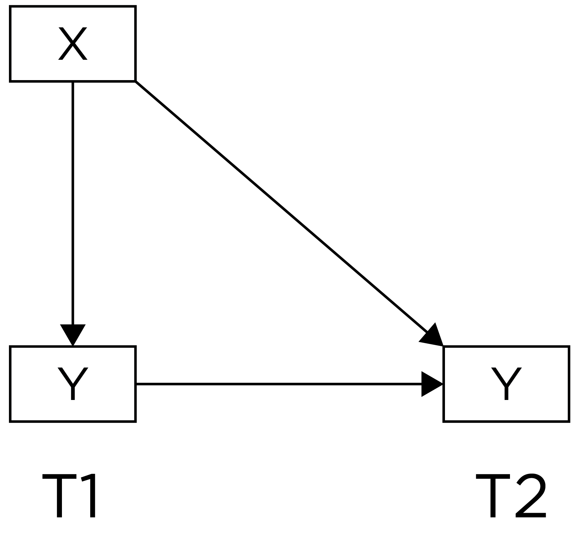
For instance, we might observe that sports drink performance before the game is associated with better player performance during the game. A lagged association has somewhat better internal validity than a cross-sectional association because we have greater evidence of temporal precedence—that the influence of the predictor precedes the outcome because the predictor was assessed before the outcome and it shows a predictive association. However, part of the association between the predictor with later levels of the outcome could be due to prior levels of the outcome that are stable across time. That is, it could be that better player performance leads players to consume more sports drink and that player performance is relatively stable across time. In such a case, it may be observed that sports drink consumption predicts later player performance even though player performance influences sports drink consumption, rather than the other way around Thus, consider an even stronger alternative—a lagged association that controls for prior levels of the outcome, as in Figure 13.3:
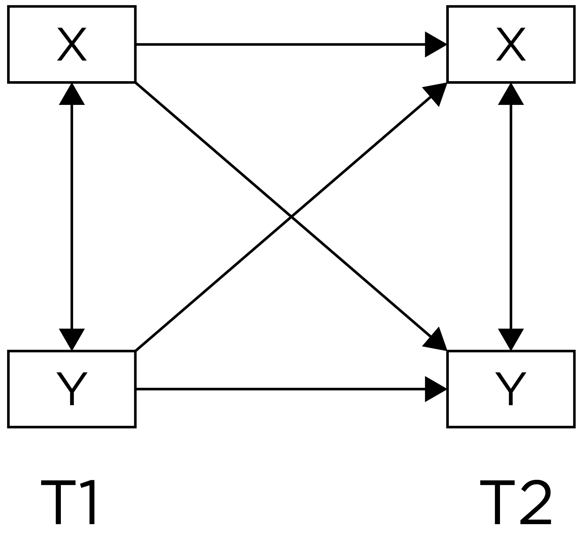
For instance, we might observe that sports drink performance before the game is associated with better player performance during the game, while controlling for prior player performance. A lagged association controlling for prior levels of the outcome has better internal validity than a lagged association that does not control for prior levels of the outcome. A lagged association that controls for prior levels further reduces the likelihood that the association owes to the reverse direction of effect, because earlier levels of the outcome are controlled. However, consider an even stronger alternative—lagged associations that control for prior levels of the outcome and that simultaneously test each direction of effect, as depicted in Figure 13.4:
Lagged associations that control for prior levels of the outcome and that simultaneously test each direction of effect provide the strongest internal validity among observational/correlational designs. Such a design can help better clarify which among the variables is the chicken and the egg—which variable is more likely to be the cause and which is more likely to be the effect. If there are bidirectional effects, such a design can also help clarify the magnitude of each direction of effect. For instance, we can simultaneously evaluate the extent to which sports drink predicts later player performance (while controlling for prior performance) and the reverse—player performance predicting later sports drink consumption (while contorlling for prior sports drink consumption).
13.5.2.2 Within-Subject Analyses
Another design feature of longitudinal designs that can lead to greater internal validity is the use of within-subject analyses, including interrupted time series designs (D’Onofrio et al., 2020). Between-subject analyses, might examine, for instance, whether players who consume more sports drink perform better on average compared to players who consume less sports drink. However, there are other between-person differences that could explain any observed between-subject associations between sports drink consumption and players performance. Another approach could be to apply within-subject analyses. For instance, you could examine whether, within the same individual, if a player consumes a sports drink, do they perform better compared to games in which they did not consume a sports drink. When we control for prior levels of the outcome in the prediction, we are evaluating whether the predictor is associated with within-person change in the outcome. Predicting within-person change provides stronger evidence consistent with causality because it uses the individual as their own control and controls for many time-invariant confounds (i.e., confounds that do not change across time). However, predicting within-person change does not, by itself, control for time-varying confounds. So, it can also be useful to control for time-varying confounds, such as by use of control variables.
13.5.2.3 Control Variables
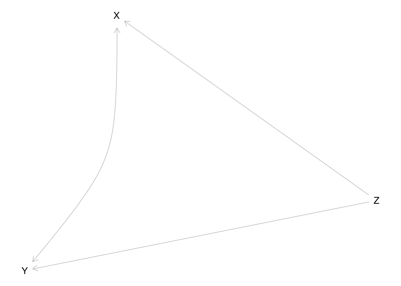
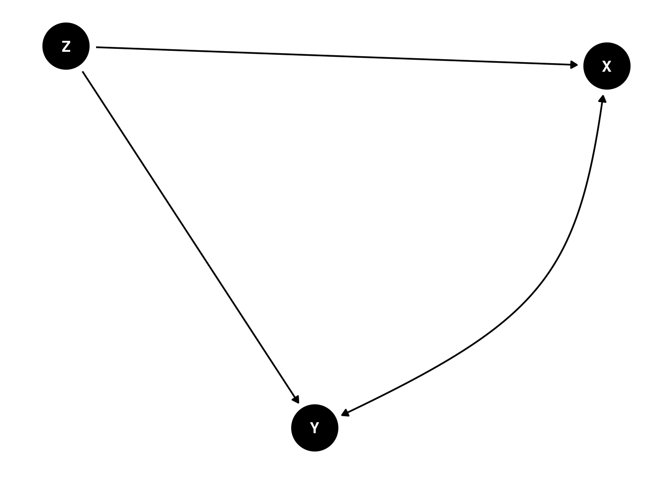
One of the plausible alternatives to the inference that X causes Y is that there are third variable confounds that influence both X and Y, thus explaining why X and Y are associated, as depicted in Figures 8.3 and 13.10. Thus, another approach that can help increase internal validity is to include plausible confounds as control variables. For instance, if a third variable such as education level might be a confound that influences both sports drink consumption and player performance, you could control for a player’s education level.
There are several ways to control for a variable:
- randomization (when possible)
- restriction
- matching
- covariate
- stratification
One way to control for a variable—and what is typically considered the most rigorous control—when possible, is to randomize (which would make it an experiment). For example, you could randomly assign players to consume sports drink during a game versus water. By randomly assigning players to each group, it is expected that, if the groups are large enough, the differences between the groups on all variables besides the independent and dependent variables will be approximately equal across both groups; thus, such an approach controls for both observed and unobserved confounds, and any difference in the dependent variable is thought to be attributable to the manipulation of the independent variable. However, sometimes a variable is not able to be manipulated for practical or ethical reasons. For instance, if you wanted to control for education level when examining the association between sports drink consumption and performance, you cannot randomly assign players to have lower educational levels (though you could possibly provide an intervention to increase the education levels of a subset of players). Thus, observational studies are also necessary.
However, in observational studies, the groups may differ on the confounding factors; for instance, due to other factors (e.g., personality, beliefs, and attitudes), people may choose (or self-select into) the level of the variable (e.g., sport drink consumption) they receive. Thus, we need to attempt to control for the confounds; however, in an observational study, we can only potentially adjust for the observed confounds, unlike in an experiment in which we can control for both observed and unobserved confounds.
A second way to control for a variable is restriction—e.g., you can select your sample so that it only includes portions/subgroups of a variable. For example, you could recruit—as participants—only those players who are college graduates.
Matching means that you match people based on the control variable. If some people consume sports drink whereas others do not, matching would mean finding—for every player included in the study who consumes sports drink—an equivalent player in terms of education who does not consume sports drink.
Another way to control for a variable is to include the variable as a covariate in the model. Inclusion of a covariate attempts to control for the variable by examining the association between the predictor variable and the outcome variable while holding the covariate variables constant. For example, if you want to control for a player’s education level in examining the association between sports drink consumption and performance, you could statistically control for player education by including the player’s education level as a covariate in predicting performance. Such a model would examine whether, when accounting for education level (by holding education level constant—i.e., partialing out the association between education level and player performance), there is an association between sports drink consumption and player performance.
Another way to control for a variable is to conduct a stratified analysis based on the variable—e.g., you can examine the association between the variables of interest within subgroups of the control variable (D’Onofrio et al., 2020). For instance, taking the example of controlling for a player’s education in examining the association between sports drink consumption and performance, you could examine the association between sports drink consumption and performance separately for various education levels: a) high school or lower, b) some college, c) college degree, d) graduate degree.
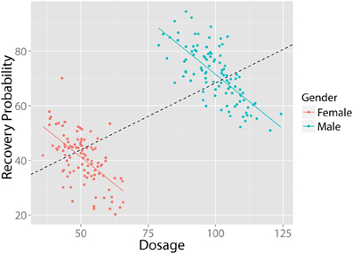
In each of these examples, you are controlling for player education for purposes of examining the effect of sports drink consumption on performance. Failure to control for important third variables can lead to erroneous conclusions, as evidenced by the association depicted in Figure 13.5, which is an example of Simpson’s paradox described in Section 12.2.2. In the example, if we did not control for gender, we would infer that there is a positive association between dosage and recovery probability. However, when we examine each men and women separately, we learn that the association between dosage and recovery probability is actually negative within each gender group. Thus, in this case, failure to control for gender would lead to false inferences about the association between dosage and recovery probability.
However, it can be problematic to control for variables indiscriminantly (Spector & Brannick, 2010; Wysocki et al., 2022). The use of causal diagrams can inform which variables are important to be included as control variables, and—just as important—which variables not to include as control variables, as described in Section 13.6. Another approach that is sometimes used to control for variables—either by using matching, or as a sample weight, or with stratification—is the use of propensity scores.
13.5.2.4 Genetically Informed Designs
Another approach to control for variables is to use genetically informed designs. Genetically informed designs allow controlling for potential genetic effects in order to more closely approximate the contributions of various environmental effects. Genetically informed designs exploit differing degrees of genetic relatedness among participants to capture the extent to which genetic factors may contribute to an outcome. The average percent of DNA shared between people of varying relationships is provided by International Society of Genetic Genealogy (2022) in Table 13.1 (archived at https://perma.cc/MK3D-DST8):
| Relationship | Average Percent of Autosomal DNA Shared by Pairs of Relatives |
|---|---|
| Monozygotic (“identical”) twins | 100% |
| Dizygotic (“fraternal”) twins | 50% |
| Parent/child | 50% |
| Full siblings | 50% |
| Grandparent/grandchild | 25% |
| Aunt-or-uncle/niece-or-nephew | 25% |
| Half-siblings | 25% |
| First cousin | 12.5% |
| Great-grandparent/great-grandchild | 12.5% |
Genetically informed designs evaluate the extent to which individuals who share greater genetic relatedness are more similar in a characteristic compared to individuals who share less genetic relatedness. For instance, researchers may compare monozygotic twins versus dizygotic twins in some outcome—a so-called “twin study”. It is assumed that the trait/outcome is attributable to genetic factors to the extent that the monozygotic twins (who share 100% of their DNA) are more similar in the trait or outcome compared to the dizygotic twins (who share on average 50% of their DNA). Alternatively, researchers could compare full siblings versus half-siblings, or they could compare full siblings versus first cousins.
Genetically informed designs are not as relevant for fantasy football analytics, but they are useful to present as one of various design features that researchers can draw upon to strengthen their ability to make causal inferences. One of the limitations of genetically informed designs is that they cannot, without inclusion of measured factors, rule out the influence of factors that are not shared by family members (D’Onofrio et al., 2020).
13.6 Causal Diagrams
13.6.1 Overview
A key tool when describing a research question or hypothesis is to create a conceptual depiction of the hypothesized causal processes. A causal diagram depicts the hypothesized causal processes that link two or more variables. A common form of causal diagrams is the directed acyclic graph (DAG). DAGs provide a helpful tool to communicate about causal questions and help identify how to avoid bias (i.e., overestimation) in associations between variables due to confounding (i.e., common causes) (Digitale et al., 2022). For instance, from a DAG, it is possible to determine what variables it is important to control for (and how)—and just as importantly, what not to control for—in order to get unbiased estimates of the effect of one variable on another variable or of the association between two variables of interest. Thus, when designing and conducting studies, it is good to get in the habit of drawing causal diagrams to make your hypotheses, knowledge, and assumptions explicit (D’Onofrio et al., 2020). Using a causal diagram (DAG), it is also valuable to specify any potential alternative hypotheses, so that the researcher can design studies to evaluate and rule out potential alternative hypotheses.
To create DAGs, you can use the R package dagitty (Textor et al., 2016, 2023) or the associated browser-based extension, DAGitty: https://dagitty.net (archived at https://perma.cc/U9BY-VZE2). Examples of various causal diagrams that could explain why X is associated with Y are in Figures 13.6, 13.8 and 13.10.
Code
Here is an alternative way of specifying the same diagram (more similar to lavaan syntax) using the ggdag package (Barrett, 2024):
Code
Code
Here is an alternative way of specifying the same diagram (more similar to lavaan syntax):
Code
Code
Here is an alternative way of specifying the same diagram (more similar to lavaan syntax):
Code
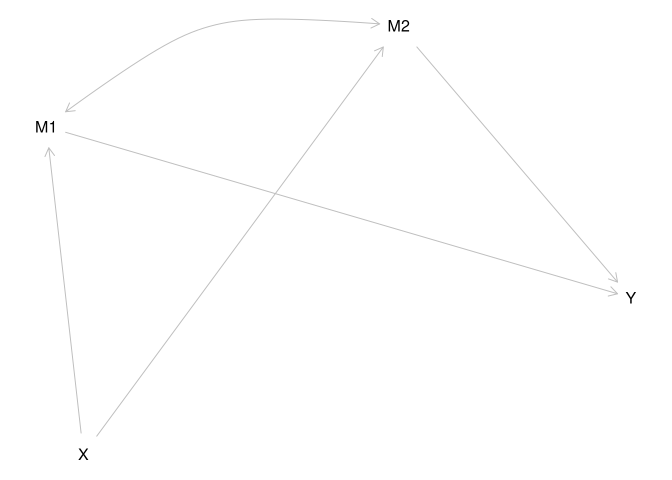
Consider another example in Figure 13.12:
Code
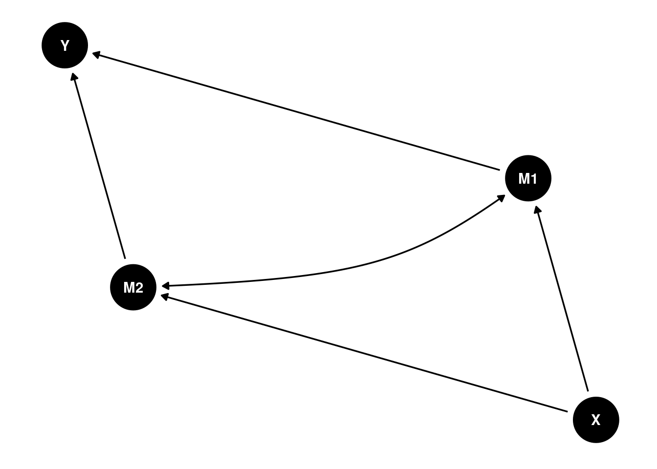
X _||_ Y | M1, M2{ M2 }In this example, X influences Y via M1 and M2 (i.e., multiple mediators), and M1 is also associated with M2. The dagitty::impliedConditionalIndependencies() function identifies variables in the causal diagram that are conditionally independent (i.e., uncorrelated) after controlling for other variables in the model. For this causal diagram, X is conditionally independent with Y because X is independent with Y when controlling for M1 and M2.
The dagitty::adjustmentSets() function identifies variables that would be necessary to control for in order to identify an unbiased estimate of the association (whether the total effect, i.e., effect = "total"; or the direct effect, i.e., effect = "direct") between two variables (exposure and outcome). In this case, to identify the unbiased association between M1 and Y, it is important to control for M2.
Here is an alternative way of specifying the same diagram (more similar to lavaan syntax) using the ggdag::dagify() and ggdag::ggdag() functions:
13.6.2 Confounding
Confounding occurs when two variables—that are both caused by another variable(s)—have a spurious or noncausal association (D’Onofrio et al., 2020). That is, two variables share a common cause, and the common cause leads the variables to be associated even though they are not causally related. The common cause—i.e., the variable that influences the two variables—is known as a confound (or confounder). Nevertheless, causal effects and confounding—though competing hypotheses—are not mutually exclusive (D’Onofrio et al., 2020). A predictor can have an association with an outcome that is partly driven by confounding and partly driven by a causal effect. A key goal, then is determining the extent to which the observed association reflects confounding versus a causal effect.
Confounding is among the most common sources of bias in observational studies in terms of accurately estimating the causal effect of one variable on another, because among all the processes that influence one’s exposure on a risk factor (i.e., predictor variable), some of the processes also likely influence the outcome variable [i.e., and are thus confounds; D’Onofrio et al. (2020)]. Two common sources of confounding that are often neglected are previous behavior and genetics (D’Onofrio et al., 2020). Part of the challenge in observational studies is that there can be known and unknown sources of confounding (D’Onofrio et al., 2020). In addition, the sources of counfounding can be either measured or unmeasured. Because some sources of confounding are likely to be unknown and/or unmeasured, it is unlikely that any single observational study can account for all sources of confounding (D’Onofrio et al., 2020). The causal diagram is thus useful for determining what sources of confounding a given study can and cannot address (D’Onofrio et al., 2020).
An example of confounding is depicted in Figure 13.14:
Code
The output indicates that player endurance (X) and field goals made (Y) are conditionally independent when accounting for stadium altitude (Z). Conditional independence refers to two variables being unassociated when controlling for other variables.
The output indicates that, to obtain an unbiased estimate of the causal association between two variables, it is necessary to control for any confounding (Lederer et al., 2019). That is, to obtain an unbiased estimate of the causal association between player endurance (X) and field goals made (Y), it is necessary to control for stadium altitude (Z).
Another challenge with confounding is that all constructs are measured with error. Thus, including a measure of a confound as a covariate in a model will only partially account for the confound. The remaining effect of the confound on the outcome (after controlling for the measured confound via a covariate) is called residual confounding (D’Onofrio et al., 2020).
13.6.2.1 Systematic Measurement Error
Another common source of bias, in terms of accurately estimating the causal effect of one variable on another, that functions similarly to confounding is systematic measurement error (as opposed to random measurement error). Systematic measurement error is measurement error that influences scores consistently for a person or across the sample. Systematic measurement error is described in Petersen (2025). Let’s consider that a researcher wants to study the effects of player stress on their happiness. The researcher selects a questionnaire that assesses player stress and a questionnaire that assesses happiness and assesses players on both. To some degree, the measurements will both be influenced by nonconstruct factors, because both measurements come from the same measurement method (questionnaire; i.e., common method bias) and from the same rater (i.e., common informant bias). People have response styles that lead them to have a tendency to rate themselves—regardless of the construct of interest—as better or worse than they actually are. For instance, Person A may rate themselves as better off in terms of stress and happiness (i.e., lower stress, higher happiness) than they actually are, whereas Person B may rate themselves as worse off in terms of stress and happiness (i.e., higher stress, lower happiness) than they actually are. Because these response styles influence both measurements and are not the construct of interest (i.e., stress or happiness), they function like confounding in that the influence both variables and can explain, to some degree, why the variables are correlated for reasons other than a causal effect of player stress on their happiness. Unlike confounding, however, systematic measurement error does not just influence observational studies—it influences experimental designs as well.
13.6.3 Mediation
Mediation can be divided into two types: full and partial. In full mediation, the mediator(s) fully account for the effect of the predictor variable on the outcome variable. In partial mediation, the mediator(s) partially but do not fully account for the effect of the predictor variable on the outcome variable.
13.6.3.1 Full Mediation
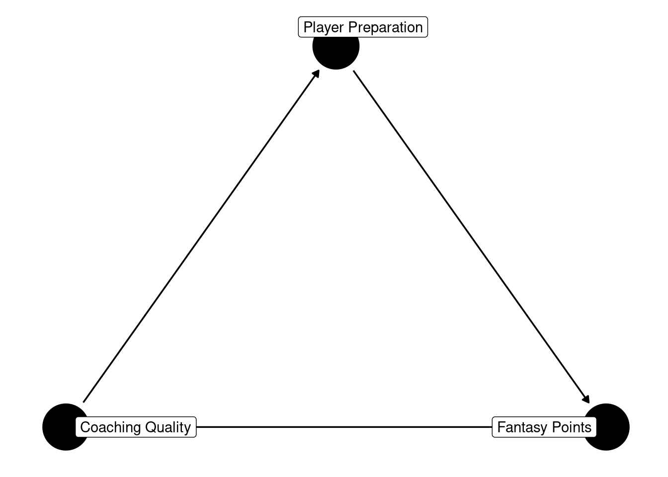
An example of full mediation is depicted in Figure 13.15:
Code
In full mediation, X and Y are conditionally independent when accounting for the mediator (Z). In this case, coaching quality (X) and fantasy points (Y) are conditionally independent when accounting for player preparation (M). In other words, in this example, player preparation is the mechanism that fully (i.e., 100%) accounts for the effect of coaching quality on players’ fantasy points.
{ m }The output indicates that, to obtain an unbiased estimate of the direct causal association between coaching quality (X) and fantasy points (Y) (i.e., the effect that is not mediated through intermediate processes), it is necessary to control for player preparation (M).
However, to obtain an unbiased estimate of the total causal association between coaching quality (X) and fantasy points (Y) (i.e., including the portion of the effect that is mediated through intermediate processes), it is important not to control for player preparation (M). When the goal is to understand the (total) causal effect of coaching quality (X) and fantasy points (Y), controlling for the mediator (player preparation; M) would be inappropriate because doing so would remove the causal effect, thus artificially reducing the estimate of the association between coaching quality (X) and fantasy points (Y) (Lederer et al., 2019).
13.6.3.2 Partial Mediation
An example of partial mediation is depicted in Figure 13.16:
Code
In partial mediation, X and Y are not conditionally independent when accounting for the mediator (Z). In this case, coaching quality (X) and fantasy points (Y) are still associated when accounting for player preparation (M). In other words, in this example, player preparation is a mechanism that partially but does not fully account for the effect of coaching quality on players’ fantasy points. That is, there are likely other mechanisms, in addition to player preparation, that collectively account for the effect of coaching quality on fantasy points. For instance, coaching quality could also influence player fantasy points through better play-calling.
{ m }As with full mediation, the output indicates that, to obtain an unbiased estimate of the direct causal association between coaching quality (X) and fantasy points (Y) (i.e., the effect that is not mediated through intermediate processes), it is necessary to control for player preparation (M).
However, as with full mediation, to obtain an unbiased estimate of the total causal association between coaching quality (X) and fantasy points (Y) (i.e., including the portion of the effect that is mediated through intermediate processes), it is important not to control for player preparation (M). When the goal is to understand the (total) causal effect of coaching quality (X) and fantasy points (Y), controlling for a mediator (player preparation; M) would be inappropriate because doing so would remove the causal effect, thus artificially reducing the estimate of the association between coaching quality (X) and fantasy points (Y) (Lederer et al., 2019).
13.6.4 Ancestors and Descendants
In a causal model, an ancestor is a variable that influences another variable, either directly or indirectly via another variable (Rohrer, 2018). A descendant is a variable that is influenced by another variable (Rohrer, 2018). In general, one should not control for descendants of the outcome variable, because doing so could eliminate the apparent effect of a legitimate cause on the outcome variable (Digitale et al., 2022). Moreover, as described above, when trying to understand the total causal effect of a predictor variable on an outcome variable, one should not control for descendants of the predictor variable that are also ancestors of the outcome variable (i.e., mediators of the effect of the predictor variable on the outcome variable) (Digitale et al., 2022).
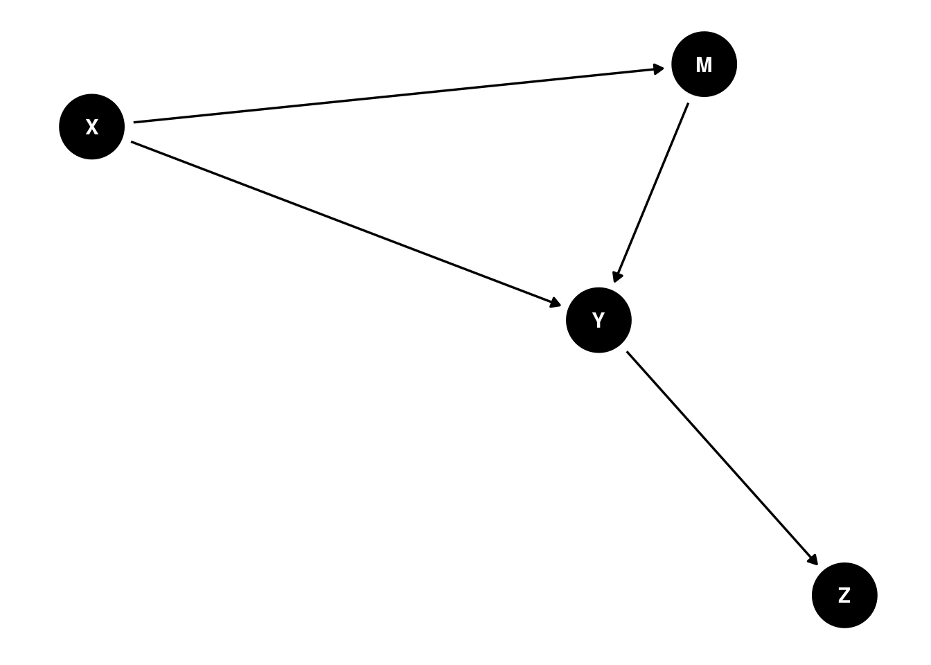
Consider the example in Figure 13.17:
Code
In this example, X and M are conditionally independent with Z when accounting for the mediator (Y).
{ M }As indicated above, one should not control for the descendant of the outcome variable; thus, one should not control for Z when examining the association between X or M and Y.
13.6.5 Collider Bias
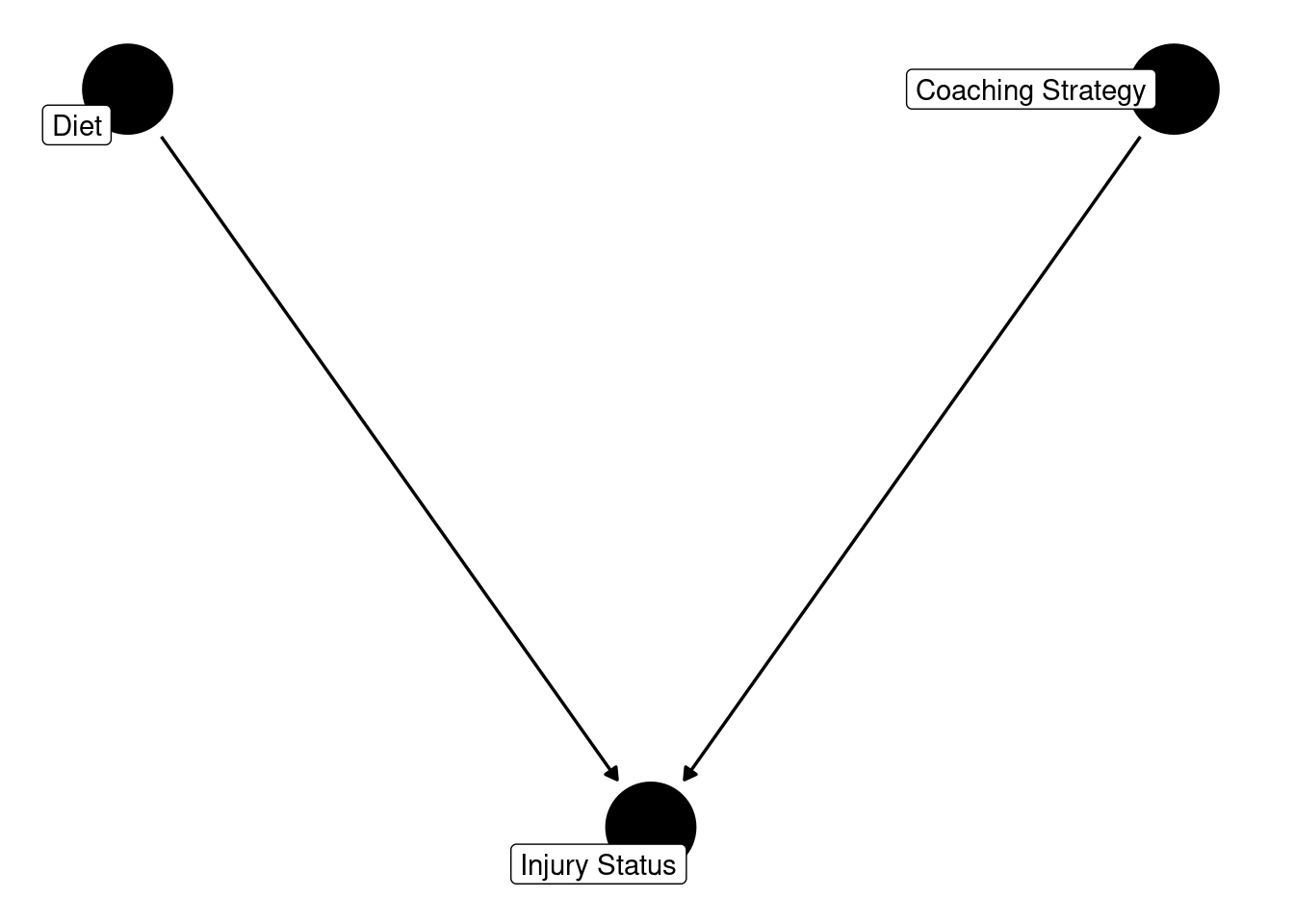
Collision occurs when two variables influence a third variable, the collider (D’Onofrio et al., 2020). That is, a collider is a variable that is caused by two other variables (i.e., a common effect). An example collision is depicted in Figures 13.18 and 13.19:
Code
In this example collision, diet (X) and coaching strategy (Y) are independent.
As the output indicates, we should not control for the collider when examining the association between the two causes of the collider. That is, we should not control for injury status (M) when examining the association between diet (X) and coaching strategy. Controlling for the collider leads to confounding and can artificially induce an association between the two causes of the collider despite no causal association between them (Lederer et al., 2019). Obtaining a distorted or artificial association between two variables due to inappropriately controlling for a collider is known as collider bias.
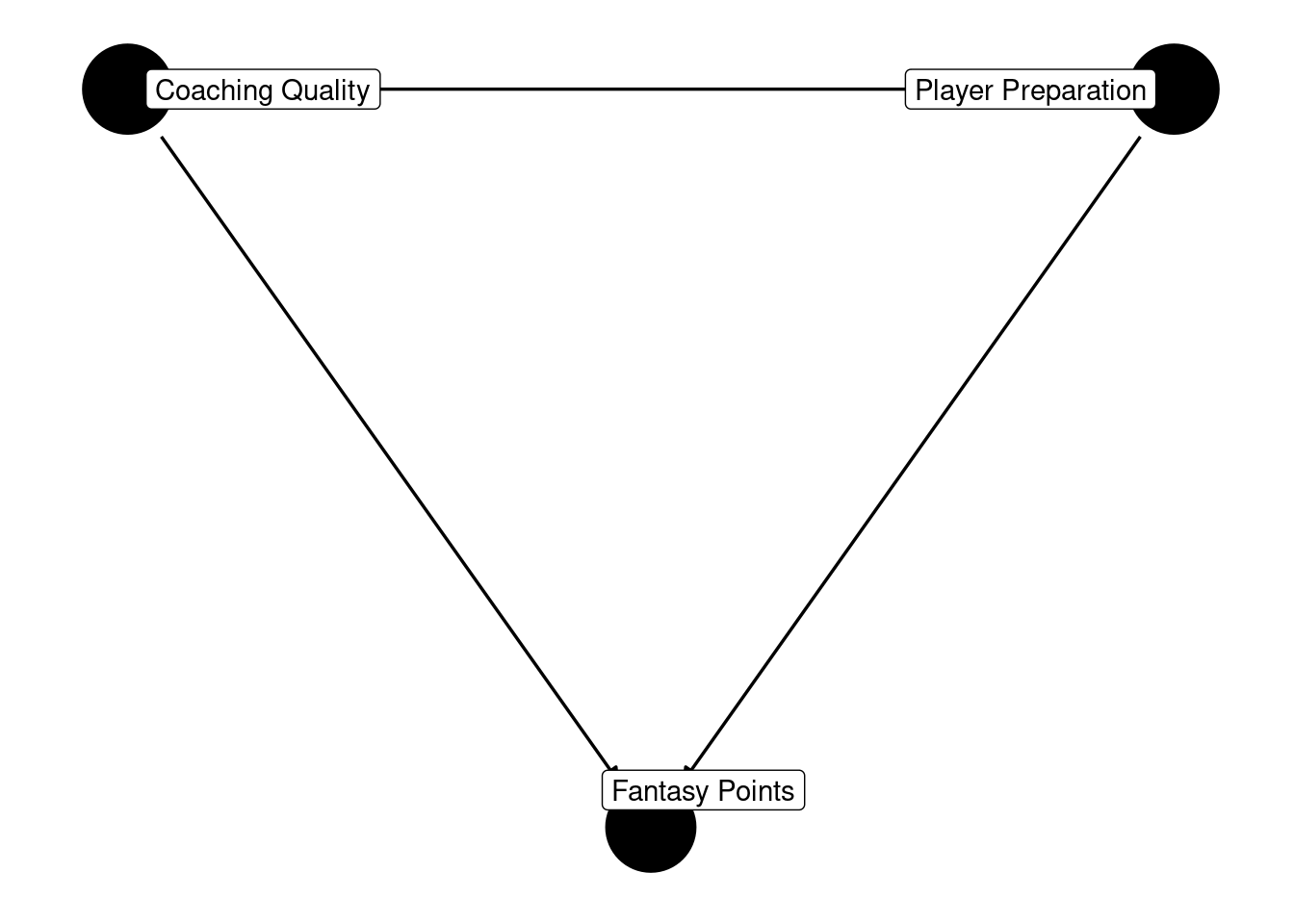
Consider another example:
Code
In this example of collider bias, there are no conditional independencies.
Again, it would be important not to control for the collider, fantasy points (M), when examining the association between coaching quality (X) and player preparation (Y). In this case, controlling for the collider would remove some of the causal effect of coaching quality on player preparation and could lead to an artificially smaller estimate of the causal effect between coaching quality and player preparation.
13.6.5.1 M-Bias
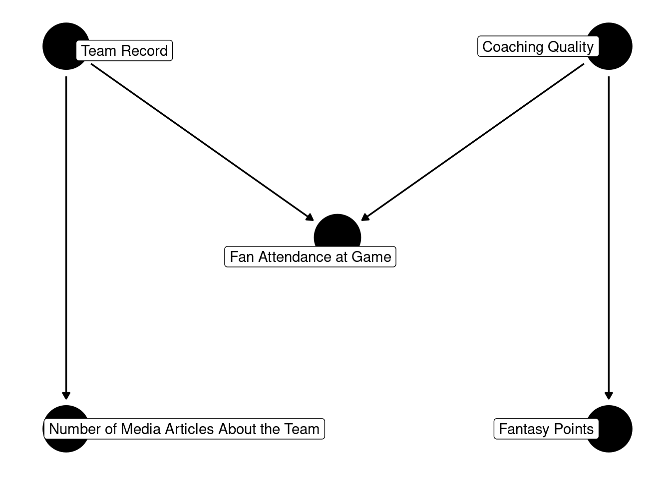
Collider bias may also occur when neither variable of interest is a direct cause of the collider (Lederer et al., 2019). M-bias is a form of collider bias that occurs when two variables that are not causally related, A and B, both influence a collider, M, and each (A and B) also influences a separate variable—e.g., A influences X and B influences Y. M-bias is so-named from the M-shape of the DAG. An example of M-bias is depicted in Figure 13.20:
Code
In this example, fan attendance is the collider that is influenced separately by the team record and the coaching quality. This is a fictitious example for purposes of demonstration; in reality, coaching quality influences the team’s record.
a _||_ b
a _||_ y
b _||_ x
m _||_ x | a
m _||_ y | b
x _||_ y
As the output indicates, there are several conditional independencies.
It is important not to control for the collider (fan attendance). If you control for the collider, you can induce an artificial association between team record and coaching quality. Moreover, because doing so induces an artificial association between team record and coaching quality, it can also induce an artificial association between the effects of team record and coaching quality: number of media articles about the team and fantasy points, respectively. That is, controlling for the collider can lead to an artificial association between X and Y that does not reflect a causal process.
13.6.5.2 Butterfly Bias
Butterfly bias occurs when both confounding and M-bias are present. Butterfly bias (aka bow-tie bias) is so-named from the butterfly shape of the DAG. In butterfly bias, the following criteria are met:
- Two variables (
AandB) influence a collider (M). - The collider influences two variables,
XandY. -
Aalso influencesX. -
Balso influencesY. -
AandBare not causally related. -
XandYare not causally related.
Or, more succinctly:
-
AinfluencesMandX. -
BinfluencesMandY. -
MinfluencesXandY.
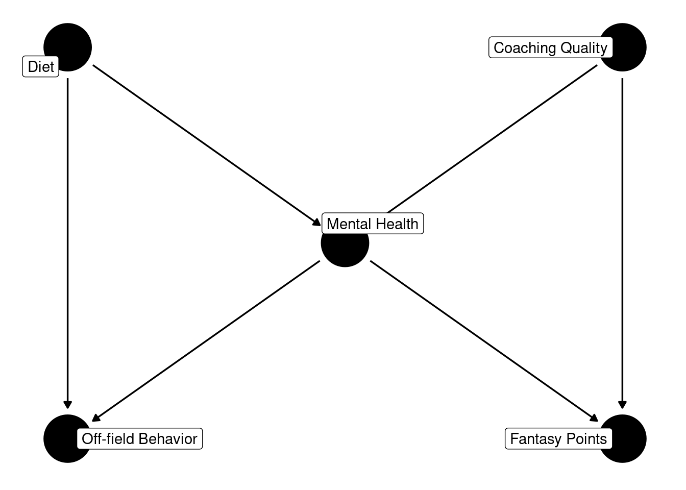
In butterfly bias, the collider (M) is also a confound. That is, a variable is both influenced by two variables and influences two variables. An example of butterfly bias is depicted in Figure 13.21:
Code
In this case, players’ mental health is a collider of their diet and the quality of the coaching they receive. In addition, players’ mental health is a confound of their off-field behavior and fantasy points.
a _||_ b
a _||_ y | b, m
b _||_ x | a, m
x _||_ y | b, m
x _||_ y | a, m
As the output indicates, there are several conditional independencies.
{ b, m }
{ a, m }
When dealing with a collider that is also a confound, controlling for either set, B and M or A and M, will provide an unbiased estimate of the association between X and Y. In this case, controlling for either a) coaching quality and mental health or b) diet and mental health—but not both sets—will yield an unbiased estimate of the association between off-field behavior and fantasy points. If you control for the both sets (M, A, and B), you can induce an artificial association between X and Y, which is called butterfly (or bow-tie) bias.
13.6.6 Selection Bias
Selection bias occurs when the selection of participants or their inclusion in analyses depends on the variables being studied (or on their colliders). For instance, if you are conducting a study on the extent to which sports drink consumption influences fantasy points, there would be selection bias if players are less likely to participate in the study if they score fewer fantasy points.
Now, consider a study in which you conduct a randomized controlled trial (RCT; i.e., an experiment) to evaluate the effect of a new medication on player performance. You randomly assign some players to take the medication and other players to take a placebo. Assume the new medication has side effects and leads many of the players who take it to drop out of the study. This is an example of attrition bias (i.e., systematic attrition). If you were to exclude these individuals from your analysis, it may make it appear that the medication led to better performance, because the players who experienced the side effect (and worse performance) dropped out of the study. Hence, conducting an analysis that excludes these players from the analysis would involve selection bias.
13.7 Summary of Variables to Control For (and Not to Control For)
In general, you should control for all confounds. In addition, it is okay to control for ancestors of the outcome variable that are not confounds or mediators. That is, it is okay to control for variables that influence Y that do not influence X and that are not influenced by X. When including these variable as control variables in a model, they are called precision variables. You do not need to include precision variables in the model because the estimate of the association is already unbiased if you have controlled for all confounds. However, including precision variables in the model reduces residual variance in the outcome variable and can yield more precise estimates (i.e., smaller standard errors) of the association between the predictor variable and outcome variable. It is also possibly okay to control for ancestors of the predictor variable that are not confounds. That is, it is possibly okay to control for variable that influence X that do not influence Y and that are not influenced by X. However, controlling for ancestors of the predictor variable (that are not confounds) can reduce precision of the estimate of the causal effect because you are reducing useful variation in X.
In addition, there are some variables that are important not to control for. It is important not to control for mediators of two variables for which you want to determine the estimate of the causal effect—unless you are interested in the direct causal effect of the predictor variable on the outcome variable above and beyond the mediator. In addition, it is is important not to control for a) descendants of the outcome variable and b) colliders (unless the collider is also a confound).
13.8 Conclusion
There are three criteria for establishing causality: 1) the cause precedes the effect. 2) The cause is related to the effect. 3) There are no other alternative explanations for the effect apart from the cause. In general, it is important to be aware of the counterfactual and to consider what would have happened if the supposed cause had not occurred. Various experimental and quasi-experimental designs and approaches can be leveraged to more closely approximate causal inferences. Longitudinal designs, within-subject analyses, inclusion of control variables, and genetically informed designs are all quasi-experimental designs that afford the researcher greater control over some possible third variable confounds. Causal diagrams can be a useful tool for identifying the proper variables to control for (and those not to control for). In general, the only variables you should control for are confounds—however, it is okay to control for ancestors of the outcome variable that are not confounds or mediators. When confounding exists, it is important to control for the confound(s). It is important not to control for mediators when interested in the total effect of the predictor variable on the outcome variable. In addition, it is important not to control for ancestors of the predictor variable or descendants of the outcome variable. When there is a collision, it is important not to control for the collider (unless the collider is also a confound).
13.9 Session Info
R version 4.6.0 (2026-04-24)
Platform: x86_64-pc-linux-gnu
Running under: Ubuntu 24.04.4 LTS

Matrix products: default
BLAS:   /usr/lib/x86_64-linux-gnu/openblas-pthread/libblas.so.3
LAPACK: /usr/lib/x86_64-linux-gnu/openblas-pthread/libopenblasp-r0.3.26.so;  LAPACK version 3.12.0

locale:
 [1] LC_CTYPE=C.UTF-8       LC_NUMERIC=C           LC_TIME=C.UTF-8
 [4] LC_COLLATE=C.UTF-8     LC_MONETARY=C.UTF-8    LC_MESSAGES=C.UTF-8
 [7] LC_PAPER=C.UTF-8       LC_NAME=C              LC_ADDRESS=C
[10] LC_TELEPHONE=C         LC_MEASUREMENT=C.UTF-8 LC_IDENTIFICATION=C

time zone: UTC
tzcode source: system (glibc)

attached base packages:
[1] stats     graphics  grDevices utils     datasets  methods   base

other attached packages:
[1] ggdag_0.2.13  dagitty_0.3-4

loaded via a namespace (and not attached):
 [1] viridis_0.6.5      generics_0.1.4     tidyr_1.3.2        stringi_1.8.7
 [5] digest_0.6.39      magrittr_2.0.5     evaluate_1.0.5     grid_4.6.0
 [9] RColorBrewer_1.1-3 fastmap_1.2.0      jsonlite_2.0.0     ggrepel_0.9.8
[13] gridExtra_2.3      purrr_1.2.2        viridisLite_0.4.3  scales_1.4.0
[17] tweenr_2.0.3       cli_3.6.6          rlang_1.2.0        graphlayouts_1.2.3
[21] polyclip_1.10-7    tidygraph_1.3.1    withr_3.0.2        cachem_1.1.0
[25] yaml_2.3.12        otel_0.2.0         tools_4.6.0        memoise_2.0.1
[29] dplyr_1.2.1        ggplot2_4.0.3      boot_1.3-32        curl_7.1.0
[33] vctrs_0.7.3        R6_2.6.1           lifecycle_1.0.5    stringr_1.6.0
[37] V8_8.2.0           htmlwidgets_1.6.4  MASS_7.3-65        ggraph_2.2.2
[41] pkgconfig_2.0.3    pillar_1.11.1      gtable_0.3.6       glue_1.8.1
[45] Rcpp_1.1.1-1.1     ggforce_0.5.0      xfun_0.57          tibble_3.3.1
[49] tidyselect_1.2.1   knitr_1.51         farver_2.1.2       htmltools_0.5.9
[53] igraph_2.3.1       labeling_0.4.3     rmarkdown_2.31     compiler_4.6.0
[57] S7_0.2.2 
