I want your feedback to make the book better for you and other readers. If you find typos, errors, or places where the text may be improved, please let me know. The best ways to provide feedback are by GitHub or hypothes.is annotations.
You can leave a comment at the bottom of the page/chapter, or open an issue or submit a pull request on GitHub: https://github.com/isaactpetersen/Fantasy-Football-Analytics-Textbook
Alternatively, you can leave an annotation using hypothes.is.
To add an annotation, select some text and then click the
symbol on the pop-up menu.
To see the annotations of others, click the
symbol in the upper right-hand corner of the page.
9 Basic Statistics
This chapter provides an overview of foundational statistical concepts.
9.1 Getting Started
9.1.1 Load Packages
9.1.2 Load Data
We created the player_stats_seasonal.RData object in Section 4.4.3.
9.2 Descriptive Statistics
Descriptive statistics are used to describe data. For instance, they may be used to describe the center, spread, or shape of the data. There are various indices of each.
9.2.1 Center
Indices to describe the center (central tendency) of a variable’s data include:
- mean (aka “average”) (i.e., \(M\) or \(\mu\))
- median
- Hodges-Lehmann statistic (aka pseudomedian)
- mode
- weighted mean
- weighted median
The mean of \(x\) (written as: \(\bar{x}\) or \(\mu_x\)) is calculated as in Equation 9.1:
\[ \bar{x} = \frac{\sum x_i}{n} = \frac{x_1 + x_2 + ... + x_n}{n} \tag{9.1}\]
That is, to compute the mean, sum all of the values and divide by the number of values (\(n\)). One issue with the mean is that it is sensitive to extreme (outlying) values. For instance, the mean of the values of 0, 0, 10, 15, 20, 30, and 1000 is 153.57. Another issue with the mean is that it may not be the same as any individual’s value (Rose, 2016)—that is, it may be unrepresentative of all of the individuals whose values comprise the average.
The median is determined as the value at the 50th percentile (i.e., the value that is higher than 50% of the values and is lower than the other 50% of values). Compared to the mean, the median is less influenced by outliers. The median of the values of 0, 0, 10, 15, 20, 30, and 1000 is 15.
The Hodges-Lehmann statistic (aka pseudomedian) is computed as the median of all pairwise means, and it is also robust to outliers. The pseudomedian can be computed using the DescTools::HodgesLehmann() function of the DescTools package (Signorell, 2025). The pseudomedian of the values of 0, 0, 10, 15, 20, 30, and 1000 is 15. The pseudomedian is an example of a robust average—an index of the center of a distribution that is less sensitive to outliers.
The mode is the most common/frequent value. The mode of the values of 0, 0, 10, 15, 20, 30, and 1000 is 0. The petersenlab package (Petersen, 2025a) contains the petersenlab::Mode() function for computing the mode of a set of data.
If you want to give some values more weight to others, you can calculate a weighted mean and a weighted median (or other quantile), while assigning a weight to each value. The petersenlab package (Petersen, 2025a) contains various functions for computing the weighted median (i.e., a weighted quantile at the 0.5 quantile, which is equivalent to the 50th percentile) based on Akinshin (2023). Because some projections are outliers, we use a trimmed version of the weighted Harrell-Davis quantile estimator for greater robustness.
Below is R code to estimate each:
- mean (
base::mean()):
- median (
stats::median()):
- Hodges-Lehmann statistic (aka pseudomedian;
DescTools::HodgesLehmann()):
- mode (
petersenlab::Mode()):
- weighted mean (
stats::weighted.mean()):
Code
[1] 50.36041- weighted median (
petersenlab::wthdquantile()):
9.2.2 Spread
Indices to describe the spread (variability or dispersion) of a variable’s data include:
- standard deviation (\(s\) or \(\sigma\))
- variance (\(s^2\) or \(\sigma^2\))
- range
- minimum and maximum (or some other quantiles)
- weighted quantiles
- interquartile range (IQR)
- median absolute deviation
- coefficient of variation
The (sample) variance of \(x\) (written as: \(s^2\)) is calculated as in Equation 9.2:
\[ s^2 = \frac{\sum (x_i - \bar{x})^2}{n-1} \tag{9.2}\]
where \(x_i\) is each data point, \(\bar{x}\) is the mean of \(x\), and \(n\) is the number of data points. The population variance divides by \(n\) rather than \(n-1\) and is written as \(\sigma^2\).
The (sample) standard deviation of \(x\) (written as: \(s\)) is calculated as in Equation 9.3:
\[ s = \sqrt{\frac{\sum (x_i - \bar{x})^2}{n-1}} \tag{9.3}\]
The population standard deviation divides by \(n\) rather than \(n-1\) and is written as \(\sigma\).
The range is calculated of \(x\) is calculated as in Equation 9.4:
\[ \text{range} = \text{maximum} - \text{minimum} \tag{9.4}\]
The interquartile range (IQR) is calculated as in Equation 9.5:
\[ \text{IQR} = Q_3 - Q_1 \tag{9.5}\]
where \(Q_3\) is the score at the third quartile (i.e., 75th percentile), and \(Q_1\) is the score at the first quartile (i.e., 25th percentile).
The median absolute deviation (MAD) is the median of all deviations from the median, and is calculated as in Equation 9.6:
\[ \text{MAD} = \text{median}(|x_i - \tilde{x}|) \tag{9.6}\]
where \(\tilde{x}\) is the median of \(x\). Compared to the standard deviation, the median absolute deviation is more robust to outliers.
The coefficient of variation (CV) accounts for the fact that variables with larger means also tend to have larger standard deviations; it is calculated as the standard deviation divided by the mean, as in Equation 6.1.
If you want to give some values more weight to others, you can calculate weighted quantiles, while assigning a weight to each value. The petersenlab package (Petersen, 2025a) contains various functions for computing weighted quantiles based on Akinshin (2023). Because some projections are outliers, we use a trimmed version of the weighted Harrell-Davis quantile estimator for greater robustness.
Below is R code to estimate each:
- standard deviation (
stats::sd()):
- variance (
stats::var()):
- range (
base::range()):
[1] -7.28 485.10Code
[1] 492.38- minimum (
base::min()) and maximum (base::max()):
[1] -7.28[1] 485.1- quantiles (in this case, the 10th and 90th quantiles;
stats::quantile()):
- weighted quantiles (in this case, the 10th and 90th quantiles;
petersenlab::wthdquantile()):
Code
[1] 2.0000 120.2906- interquartile range (IQR;
stats::IQR()):
- median absolute deviation (
stats::mad()):
- coefficient of variation:
9.2.3 Shape
Indices to describe the shape of a variable’s data include:
- skewness
- kurtosis
The skewness represents the degree of asymmetry of a distribution around its mean. Positive skewness (right-skewed) reflects a longer or heavier right-tailed distribution, whereas negative skewness (left-skewed) reflects a longer or heavier left-tailed distribution. Fantasy points tend to be positively skewed.
The kurtosis reflects the extent of extreme (outlying) values in a distribution relative to a normal distribution (or bell curve). A mesokurtic distribution (with a kurtosis value near zero) reflects a normal amount of tailedness. Positive kurtosis values reflect a leptokurtic distribution, where there are heavier tails and a sharper peak than a normal distribution, indicating more frequent extreme values. Negative kurtosis values reflect a platykurtic distribution, where there are lighter tails and a flatter peak than a normal distribution, indicating fewer extreme values. Fantasy points tend to have a leptokurtic distribution.
Below is R code to estimate each using the psych::skew() and psych::kurtosis() functions of the psych package (Revelle, 2025):
- skewness (
psych::skew()):
- kurtosis (
psych::kurtosi()):
9.2.4 Combination
To estimate multiple indices of center, spread, and shape of the data, you can use the following code:
Code
player_stats_seasonal %>%
  dplyr::select(age, years_of_experience, fantasyPoints) %>%
  dplyr::summarise(across(
      everything(),
      .fns = list(
        n = ~ length(na.omit(.)),
        missingness = ~ mean(is.na(.)) * 100,
        M = ~ mean(., na.rm = TRUE),
        SD = ~ sd(., na.rm = TRUE),
        min = ~ min(., na.rm = TRUE),
        max = ~ max(., na.rm = TRUE),
        q10 = ~ quantile(., .10, na.rm = TRUE), # 10th quantile
        q90 = ~ quantile(., .90, na.rm = TRUE), # 90th quantile
        range = ~ max(., na.rm = TRUE) - min(., na.rm = TRUE),
        IQR = ~ IQR(., na.rm = TRUE),
        MAD = ~ mad(., na.rm = TRUE),
        CV = ~ sd(., na.rm = TRUE) / mean(., na.rm = TRUE),
        median = ~ median(., na.rm = TRUE),
        pseudomedian = ~ DescTools::HodgesLehmann(., na.rm = TRUE),
        mode = ~ petersenlab::Mode(., multipleModes = "mean"),
        skewness = ~ psych::skew(., na.rm = TRUE),
        kurtosis = ~ psych::kurtosi(., na.rm = TRUE)),
      .names = "{.col}.{.fn}")) %>%
    tidyr::pivot_longer(
      cols = everything(),
      names_to = c("variable","index"),
      names_sep = "\\.") %>%
    tidyr::pivot_wider(
      names_from = index,
      values_from = value)
9.2.5 Interactive Visualization
You can use the following interactive graph to visualize various distributions according to a specified center (mean), spread (standard deviation), and shape (skewness and kurtosis). Try varying the standard deviation, skewness, and kurtosis to see the impact of each. The interactive graph was created using the shiny (Chang et al., 2024) and PearsonDS (Becker & Klößner, 2025) packages. The source code for interactive graph is here: https://github.com/isaactpetersen/DistributionVisualizer.
9.3 Scores and Scales
There are many different types of scores and scales. This book focuses on raw scores and z scores. For information on other scores and scales, including percentile ranks, T scores, standard scores, scaled scores, and stanine scores, see here: https://isaactpetersen.github.io/Principles-Psychological-Assessment/scoresScales.html#scoreTransformation (Petersen, 2025b).
9.3.1 Raw Scores
Raw scores are the original data on the original metric. Thus, raw scores are considered unstandardized. For example, raw scores that represent the players’ age may range from 20 to 40. Raw scores depend on the construct and unit; thus raw scores may not be comparable across variables.
9.3.2 z Scores
z scores have a mean of zero and a standard deviation of one. z scores are frequently used to render scores across variables more comparable. Thus, z scores are considered a form of a standardized score.
z scores are calculated using Equation 9.7:
\[ z = \frac{x - \bar{x}}{s_x} \tag{9.7}\]
where \(x\) is the observed score, \(\bar{x}\) is the mean observed score, and \(s_x\) is the standard deviation of the observed scores.
You can easily convert a variable to a z score using the base::scale() function:
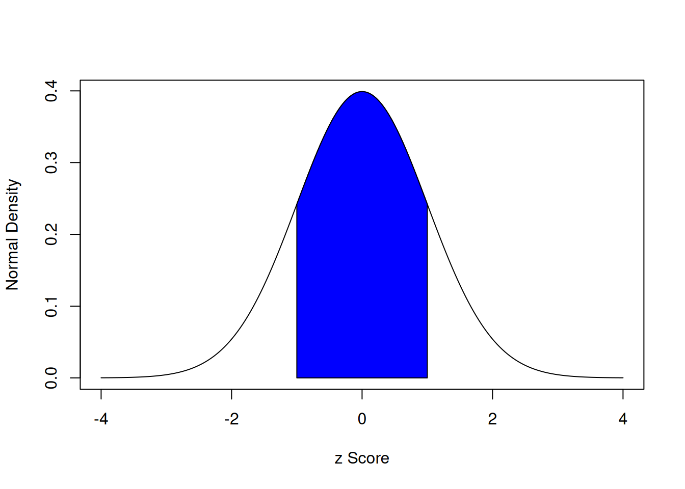
With a standard normal curve, 68% of scores fall within one standard deviation of the mean. 95% of scores fall within two standard deviations of the mean. 99.7% of scores fall within three standard deviations of the mean.
The area under a normal curve within one standard deviation of the mean is calculated below using the stats::pnorm() function, which calculates the cumulative density function for a normal curve.
The area under a normal curve within one standard deviation of the mean is depicted in Figure 9.1.
Code
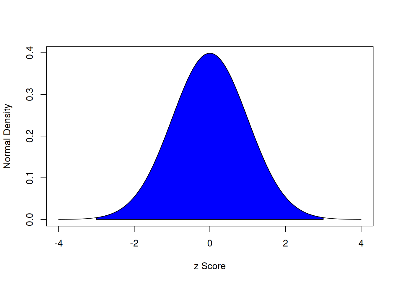
The area under a normal curve within two standard deviations of the mean is calculated below:
The area under a normal curve within two standard deviations of the mean is depicted in Figure 9.2.
Code

The area under a normal curve within three standard deviations of the mean is calculated below:
The area under a normal curve within three standard deviations of the mean is depicted in Figure 9.3.
Code
If you want to determine the z score associated with a particular percentile in a normal distribution, you can use the stats::qnorm() function. For instance, the z score associated with the 37th percentile is:
9.4 Inferential Statistics
Inferential statistics are used to draw inferences regarding whether there is (a) a difference in level on variable across groups or (b) an association between variables. For instance, inferential statistics may be used to evaluate whether Quarterbacks tend to have longer careers compared to Running Backs. Or, they could be used to evaluate whether number of carries is associated with injury likelihood. To apply inferential statistics, we make use of the null hypothesis (\(H_0\)) and the alternative hypothesis (\(H_1\)).
9.4.1 Null Hypothesis Significance Testing
To draw statistical inferences, the frequentist statistics paradigm leverages null hypothesis significance testing. Frequentist statistics is the most widely used statistical paradigm. However, frequentist statistics is not the only statistical paradigm. Other statistical paradigms exist, including Bayesian statistics, which is based on Bayes’ theorem. This chapter focuses on the frequentist approach to hypothesis testing, known as null hypothesis significance testing. We discuss Bayesian statistics in Chapter 16.
9.4.1.1 Null Hypothesis (\(H_0\))
When testing whether there are differences in level across groups on a variable of interest, the null hypothesis (\(H_0\)) is that there is no difference in level across groups. For instance, when testing whether Quarterbacks tend to have longer careers compared to Running Backs, the null hypothesis (\(H_0\)) is that Quarterbacks do not systematically differ from Running Backs in the length of their career.
When testing whether there is an association between variables, the null hypothesis (\(H_0\)) is that there is no association between the variables. For instance, when testing whether number of carries is associated with injury likelihood, the null hypothesis (\(H_0\)) is that there is no association between number of carries and injury likelihood.
9.4.1.2 Alternative Hypothesis (\(H_1\))
The alternative hypothesis (\(H_1\)) is the researcher’s hypothesis that they want to evaluate. An alternative hypothesis (\(H_1\)) might be directional (i.e., one-sided) or non-directional (i.e., two-sided).
Directional hypotheses specify a particular direction, such as which group will have larger scores or which direction (positive or negative) two variables will be associated. Examples of directional hypotheses include:
- Quarterbacks have longer careers compared to Running Backs
- Number of carries is positively associated with injury likelihood
Non-directional hypotheses do not specify a particular direction. For instance, non-directional hypotheses may state that two groups differ but do not specify which group will have larger scores. Or, non-directional hypotheses may state that two variables are associated but do not state what the sign is of the association—i.e., positive or negative. Examples of non-directional hypotheses include:
- Quarterbacks differ in the length of their careers compared to Running Backs
- Number of carries is associated with injury likelihood
9.4.1.3 Statistical Significance
Statistical significance is the reliability (i.e., consistency) of an effect, and it is evaluated with the p-value. The p-value does not represent the probability that you observed the result by chance. The p-value represents a conditional probability—it examines the probability of one event given another event. In particular, the p-value evaluates the likelihood that you would detect a result as at least as extreme as the one observed (in terms of the magnitude of the difference or of the association) given that the null hypothesis (\(H_0\)) is true.
This can be expressed in conditional probability notation, \(P(A | B)\), which is the probability (likelihood) of event A occurring given that event B occurred (or given condition B).
The conditional probability notation for a left-tailed directional test (i.e., Quarterbacks have shorter careers than Running Backs; or number of carries is negatively associated with injury likelihood) is in Equation 9.8.
\[ p\text{-value} = P(T \le t | H_0) \tag{9.8}\]
where \(T\) is the test statistic of interest (e.g., the distribution of \(t\)-, \(r-\), or \(F\) values, depending on the test) and \(t\) is the observed test statistic (e.g., \(t\)-, \(r-\), or \(F\)-coefficient, depending on the test).
The conditional probability notation for a right-tailed directional test (i.e., Quarterbacks have longer careers than Running Backs; or number of carries is positively associated with injury likelihood) is in Equation 9.9.
\[ p\text{-value} = P(T \ge t | H_0) \tag{9.9}\]
The conditional probability notation for a two-tailed non-directional test (i.e., Quarterbacks differ in the length of their careers compared to Running Backs; or number of carries is associated with injury likelihood) is in Equation 9.10.
\[ p\text{-value} = 2 \times \text{min}(P(T \le t | H_0), P(T \ge t | H_0)) \tag{9.10}\]
where min(a, b) is the smaller number of a and b.
If the distribution of the test statistic is symmetric around zero, the p-value for the two-tailed non-directional test simplifies to Equation 9.11.
\[ p\text{-value} = 2 \times P(T \ge |t| | H_0) \tag{9.11}\]
Nevertheless, to be conservative (i.e., to avoid false positive/Type I errors), many researchers use two-tailed p-values regardless whether their hypothesis is one- or two-tailed.
For a test of group differences, the p-value evaluates the likelihood that you would observe a difference as large or larger than the one you observed between the groups if there were no systematic difference between the groups in the population, as depicted in Figure 9.4.
Code
set.seed(52242)

nObserved <- 1000
nPopulation <- 1000000

observedGroups <- data.frame(
  score = c(rnorm(nObserved, mean = 47, sd = 3), rnorm(nObserved, mean = 52, sd = 3)),
  group = as.factor(c(rep("Group 1", nObserved), rep("Group 2", nObserved)))
)

populationGroups <- data.frame(
  score = c(rnorm(nPopulation, mean = 50, sd = 3.03), rnorm(nPopulation, mean = 50, sd = 3)),
  group = as.factor(c(rep("Group 1", nPopulation), rep("Group 2", nPopulation)))
)

ggplot2::ggplot(
  data = observedGroups,
  mapping = aes(
    x = score,
    fill = group,
    color = group
  )
) +
  geom_density(alpha = 0.5) +
  scale_color_manual(values = c("red", "blue")) +
  scale_fill_manual(values = c("red","blue")) +
  geom_vline(xintercept = mean(observedGroups$score[which(observedGroups$group == "Group 1")])) +
  geom_vline(xintercept = mean(observedGroups$score[which(observedGroups$group == "Group 2")])) +
  ggplot2::labs(
    x = "Score",
    y = "Frequency",
    title = "What is the probability my data would look like this..."
  ) +
  ggplot2::theme_classic(
    base_size = 16) +
  ggplot2::theme(
    legend.title = element_blank(),
    axis.text.x = element_blank(),
    axis.ticks.x = element_blank(),
    axis.text.y = element_blank(),
    axis.ticks.y = element_blank(),
    #plot.title.position = "plot"
    legend.position = "inside",
    legend.margin = margin(0, 0, 0, 0),
    legend.justification.top = "left",
    legend.justification.left = "top",
    legend.justification.bottom = "right",
    legend.justification.inside = c(1, 1),
    legend.location = "plot")

ggplot2::ggplot(
  data = populationGroups,
  mapping = aes(
    x = score,
    fill = group,
    color = group
  )
) +
  geom_density(alpha = 0.5) +
  scale_color_manual(values = c("red", "blue")) +
  scale_fill_manual(values = c("red","blue")) +
  geom_vline(xintercept = mean(populationGroups$score[which(populationGroups$group == "Group 1")])) +
  geom_vline(xintercept = mean(populationGroups$score[which(populationGroups$group == "Group 2")])) +
  ggplot2::labs(
    x = "Score",
    y = "Frequency",
    title = "...if in the population, the groups were really this:"
  ) +
  ggplot2::theme_classic(
    base_size = 16) +
  ggplot2::theme(
    legend.title = element_blank(),
    axis.text.x = element_blank(),
    axis.ticks.x = element_blank(),
    axis.text.y = element_blank(),
    axis.ticks.y = element_blank(),
    #plot.title.position = "plot",
    legend.position = "inside",
    legend.margin = margin(0, 0, 0, 0),
    legend.justification.top = "left",
    legend.justification.left = "top",
    legend.justification.bottom = "right",
    legend.justification.inside = c(1, 1),
    legend.location = "plot")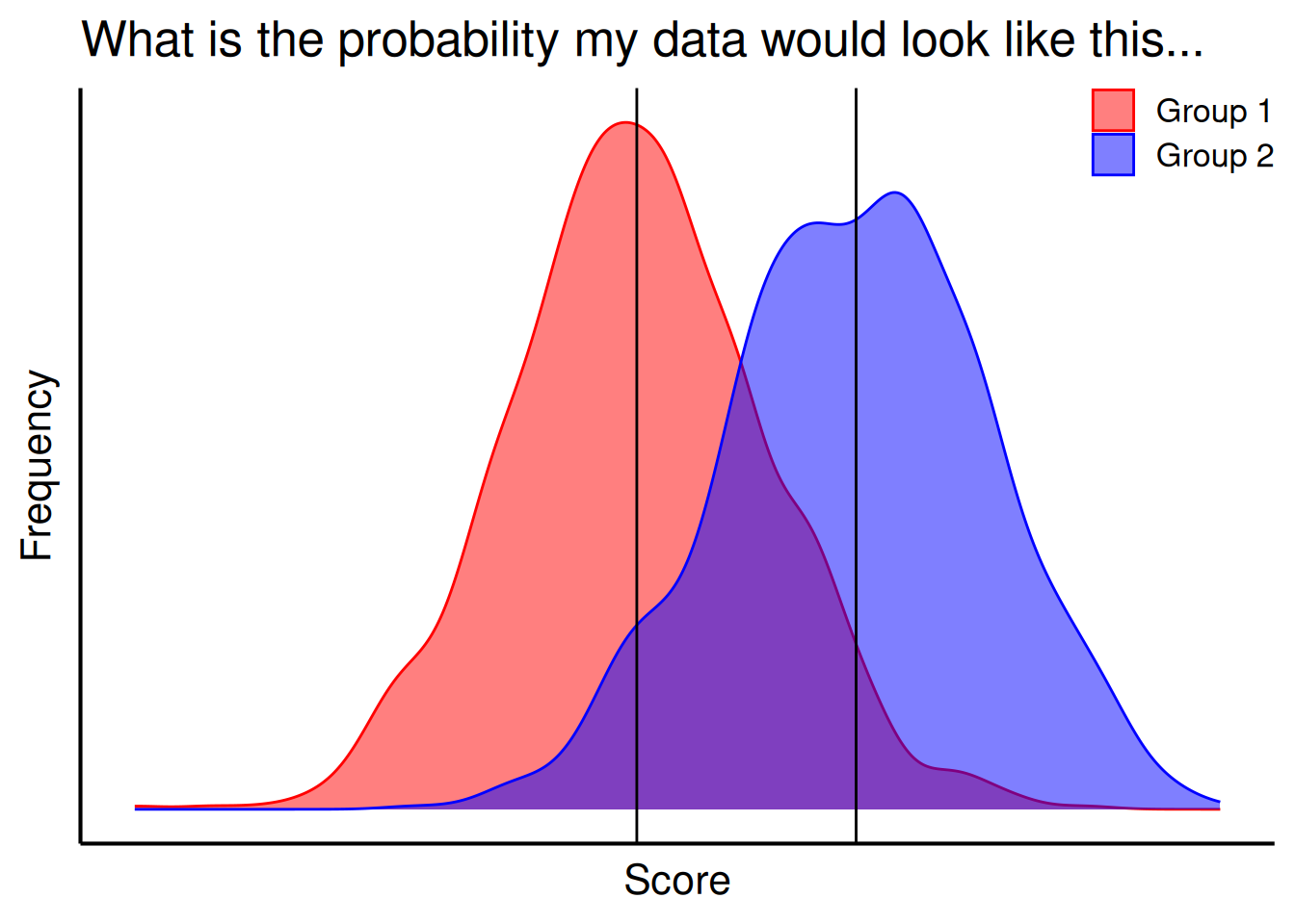
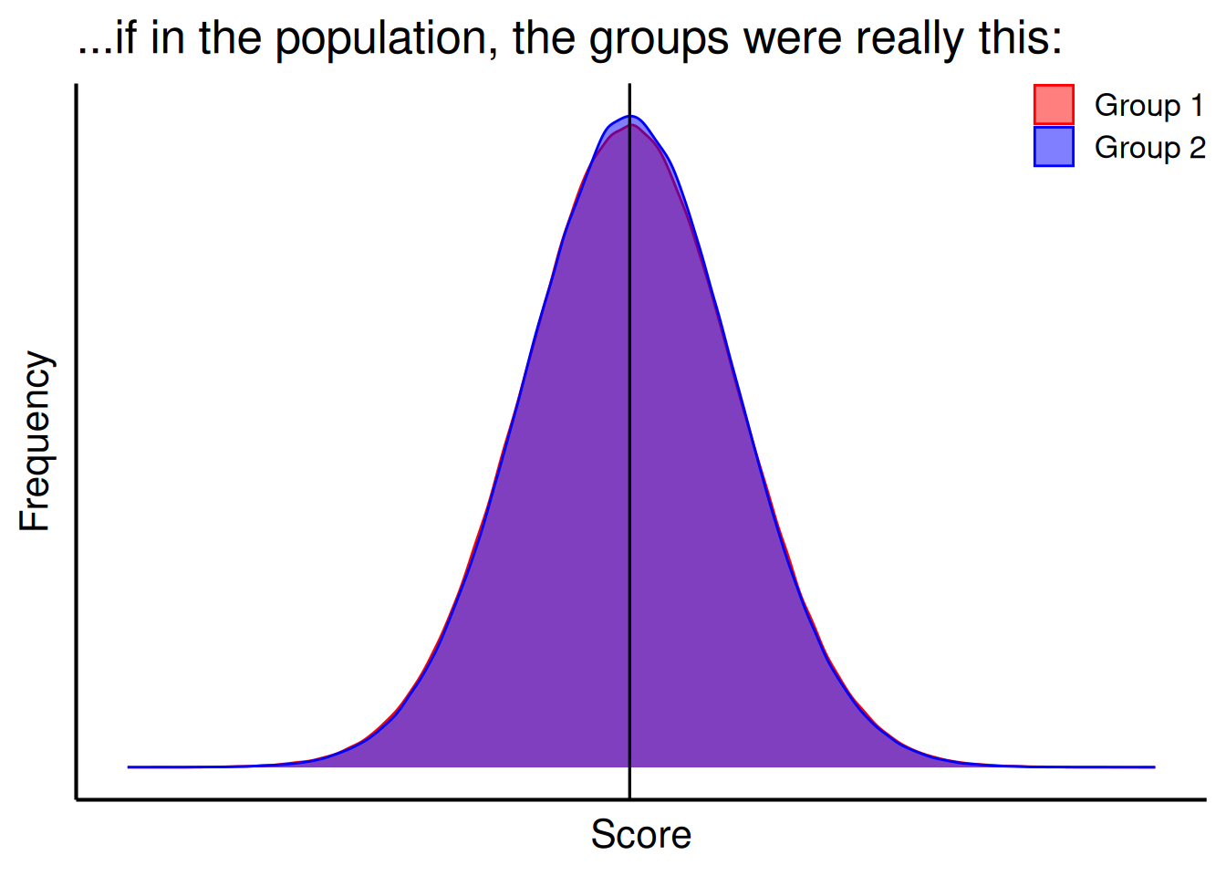
For instance, when evaluating whether Quarterbacks have longer careers than Running Backs, and you observed a mean difference of 0.03 years, the p-value evaluates the likelihood that you would observe a difference as large or larger than 0.03 years between the groups if, in truth among all Quarterbacks and Running Backs in the NFL, Quarterbacks do not differ from Running Backs in terms of the length of their career.
For a test of whether two variables are associated, the p-value evaluates the likelihood that you would observe an association as strong or stronger than the one you observed if there were no actual association between the variables in the population, as depicted in Figure 9.5.
Code
set.seed(52242)

observedCorrelation <- 0.9

correlations <- data.frame(criterion = rnorm(2000))
correlations$sample <- NA
correlations$sample[1:100] <- complement(correlations$criterion[1:100], observedCorrelation)
correlations$population <- complement(correlations$criterion, 0)

ggplot2::ggplot(
  data = correlations,
  mapping = aes(
    x = sample,
    y = criterion
  )
) +
  geom_point() +
  geom_smooth(method = "lm") +
  scale_x_continuous(
    limits = c(-3.5,3)
  ) +
  annotate(
    x = 0,
    y = 4,
    label = paste("italic(r) != ", 0, sep = ""),
    parse = TRUE,
    geom = "text",
    size = 7) +
  labs(
    x = "Predictor Variable",
    y = "Outcome Variable",
    title = "What is the probability my data would look like this..."
  ) +
  theme_classic(
    base_size = 16) +
  theme(
    legend.title = element_blank(),
    axis.text.x = element_blank(),
    axis.ticks.x = element_blank(),
    axis.text.y = element_blank(),
    axis.ticks.y = element_blank())

ggplot2::ggplot(
  data = correlations,
  mapping = aes(
    x = population,
    y = criterion
  )
) +
  geom_point() +
  geom_smooth(
    method = "lm",
    se = FALSE) +
  scale_x_continuous(
    limits = c(-2.5,2.5)
  ) +
  annotate(
    x = 0,
    y = 4,
    label = paste("italic(r) == '", "0.00", "'", sep = ""),
    parse = TRUE,
    geom = "text",
    size = 7) +
  labs(
    x = "Predictor Variable",
    y = "Outcome Variable",
    title = "...if in the population, the association was really this:"
  ) +
  theme_classic(
    base_size = 16) +
  theme(
    legend.title = element_blank(),
    axis.text.x = element_blank(),
    axis.ticks.x = element_blank(),
    axis.text.y = element_blank(),
    axis.ticks.y = element_blank())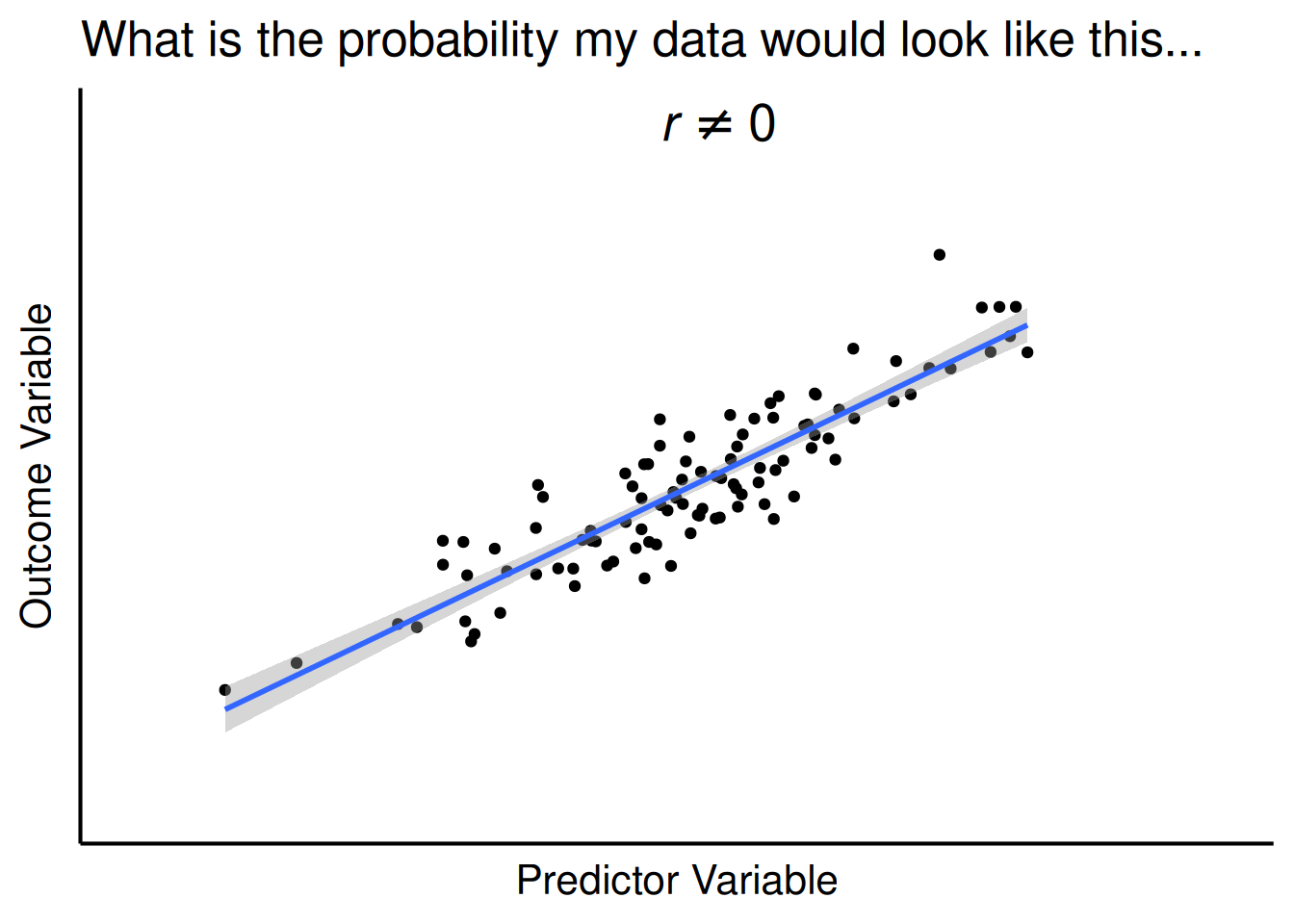
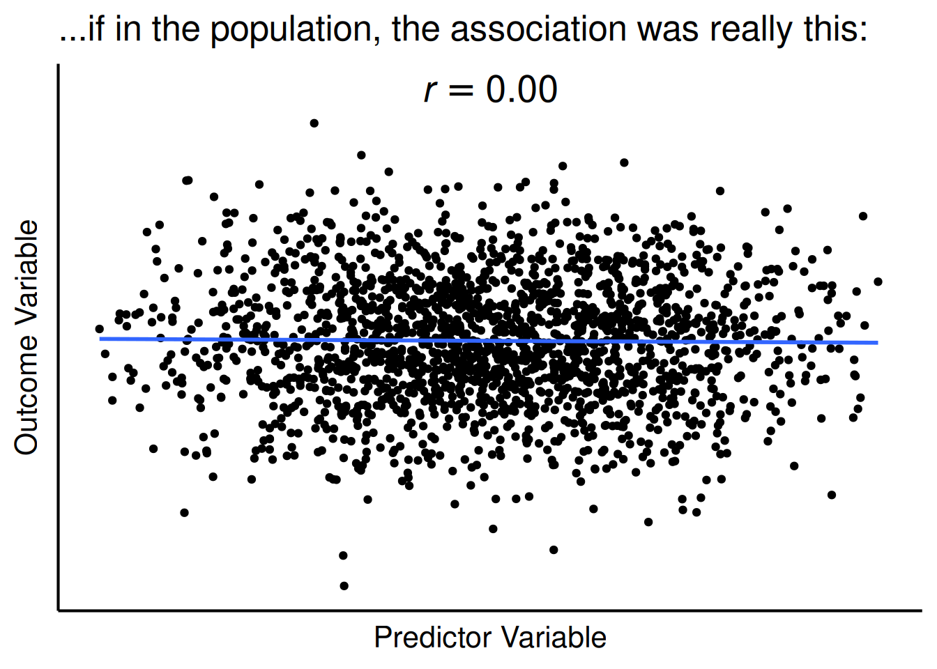
For instance, when evaluating whether number of carries is positively associated with injury likelihood, and you observed a correlation coefficient of \(r = .25\) between number of carries and injury likelihood, the p-value evaluates the likelihood that you would observe a correlation as strong or stronger than \(r = .25\) between the variables if, in truth among all NFL Running Backs, number of carries is not associated with injury likelihood.
Using what is called null-hypothesis significance testing (NHST), we consider an effect to be statistically significant if the p-value is less than some threshold, called the alpha level. In science, we typically want to be conservative because a false positive (i.e., Type I error) is considered more problematic than a false negative (i.e., Type II error). That is, we would rather say an effect does not exist when it really does than to say an effect does exist when it really does not. Thus, we typically set the alpha level to a low value, commonly .05. Then, we would consider an effect to be statistically significant if the p-value is less than .05. That is, there is a small chance (5%; or 1 in 20 times) that we would observe an effect at least as extreme as the effect observed, if the null hypothesis were true. So, you might expect around 5% of tests where the null hypothesis is true to be statistically significant just by chance. We could lower the rate of Type II (i.e., false negative) errors—i.e., we could detect more effects—if we set the alpha level to a higher value (e.g., .10); however, raising the alpha level would raise the possibility of Type I (false positive) errors.
If the p-value is less than .05, we reject the null hypothesis (\(H_0\)) that there was no difference or association. Thus, we conclude that there was a statistically significant (non-zero) difference or association. If the p-value is greater than .05, we fail to reject the null hypothesis; the difference/association was not statistically significant. Thus, we do not have confidence that there was a difference or association. However, we do not accept the null hypothesis; it could be there we did not observe an effect because we did not have adequate power to detect the effect—e.g., if the effect size was small, the data were noisy, and the sample size was small and/or unrepresentative.
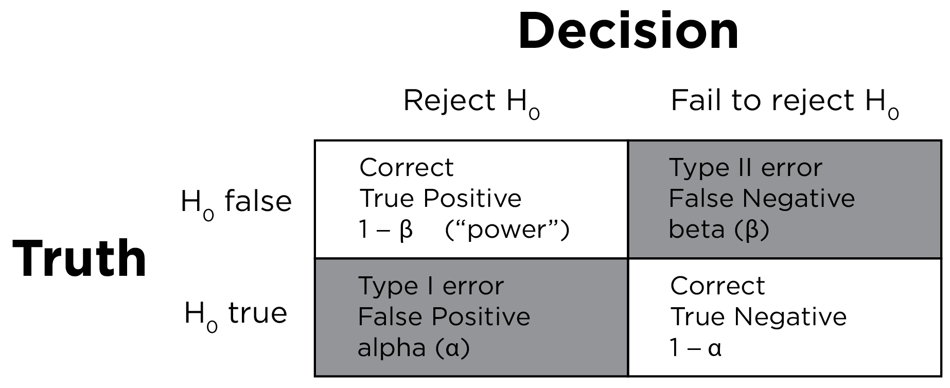
There are four general possibilities of decision making outcomes when performing null-hypothesis significance testing:
- We (correctly) reject the null hypothesis when it is in fact false (\(1 - \beta\)). This is a true positive. For instance, we may correctly determine that Quarterbacks have longer careers than Running Backs.
- We (correctly) fail to reject the null hypothesis when it is in fact true (\(1 - \alpha\)). This is a true negative. For instance, we may correctly determine that Quarterbacks do not have longer careers than Running Backs.
- We (incorrectly) reject the null hypothesis when it is in fact true (\(\alpha\)). This is a false positive. When performing null hypothesis testing, a false positive is known as a Type I error. For instance, we may incorrectly determine that Quarterbacks have longer careers than Running Backs when, in fact, Quarterbacks and Running Backs do not differ in their career length.
- We (incorrectly) fail to reject the null hypothesis when it is in fact false (\(\beta\)). This is a false negative. When performing null hypothesis testing, a false negative is known as a Type II error. For instance, we may incorrectly determine that Quarterbacks and Running Backs do not differ in their career length when, in fact, Quarterbacks have longer careers than Running Backs.
A two-by-two confusion matrix for null-hypothesis significance testing is in Figure 9.6.
In statistics, power is the probability of detecting an effect, if, in fact, the effect exists. Otherwise said, power is the probability of rejecting the null hypothesis, if, in fact, the null hypothesis is false. Power is influenced by several variables:
- the sample size (N): the larger the N, the greater the power
- for group comparisons, the power depends on the sample size of each group
- the effect size: the larger the effect, the greater the power
- for group comparisons, larger effect sizes reflect:
- larger between-group variance, and
- smaller within-group variance (i.e., strong measurement precision, i.e., reliability)
- for group comparisons, larger effect sizes reflect:
- the alpha level: the researcher specifies the alpha level (though it is typically set at .05); the higher the alpha level, the greater the power; however, the higher we set the alpha level, the higher the likelihood of Type I errors (false positives)
- one- versus two-tailed tests: one-tailed tests have higher power than two-tailed tests
- within-subject versus between-subject comparisons: within-subject designs tend to have greater power than between-subject designs
A plot of statistical power is in Figure 9.7, as adapted from Magnusson (2013) (archived at https://perma.cc/FG3J-85L6).
Code
m1 <- 0  # mu H0
sd1 <- 1.5 # sigma H0
m2 <- 3.5 # mu HA
sd2 <- 1.5 # sigma HA

z_crit <- qnorm(1-(0.05/2), m1, sd1)

# set length of tails
min1 <- m1-sd1*4
max1 <- m1+sd1*4
min2 <- m2-sd2*4
max2 <- m2+sd2*4
# create x sequence
x <- seq(min(min1,min2), max(max1, max2), .01)
# generate normal dist #1
y1 <- dnorm(x, m1, sd1)
# put in data frame
df1 <- data.frame("x" = x, "y" = y1)
# generate normal dist #2
y2 <- dnorm(x, m2, sd2)
# put in data frame
df2 <- data.frame("x" = x, "y" = y2)

# Alpha polygon
y.poly <- pmin(y1,y2)
poly1 <- data.frame(x=x, y=y.poly)
poly1 <- poly1[poly1$x >= z_crit, ]
poly1 <- rbind(poly1, c(z_crit, 0))  # add lower-left corner

# Beta polygon
poly2 <- df2
poly2 <- poly2[poly2$x <= z_crit,]
poly2 <- rbind(poly2, c(z_crit, 0))  # add lower-left corner

# power polygon; 1-beta
poly3 <- df2
poly3 <- poly3[poly3$x >= z_crit,]
poly3 <- rbind(poly3, c(z_crit, 0))  # add lower-left corner

# combine polygons
poly1$id <- 3 # alpha, give it the highest number to make it the top layer
poly2$id <- 2 # beta
poly3$id <- 1 # power; 1 - beta
poly <- rbind(poly1, poly2, poly3)
poly$id <- factor(poly$id,  labels = c("power", "beta", "alpha"))

# plot with ggplot2
ggplot(
  poly,
  aes(
    x,
    y,
    fill = id,
    group = id)) +
  geom_polygon(
    show.legend = FALSE,
    alpha = I(8/10)) +
  # add line for treatment group
  geom_line(
    data = df1,
    aes(
      x,
      y,
      color = "H0",
      group = NULL,
      fill = NULL),
    linewidth = 1.5,
    show.legend = FALSE) +
  # add line for treatment group. These lines could be combined into one dataframe.
  geom_line(
    data = df2,
    aes(
      color = "HA",
      group = NULL,
      fill = NULL),
    linewidth = 1.5,
    show.legend = FALSE) +
  # add vlines for z_crit
  geom_vline(
    xintercept = z_crit,
    linewidth = 1,
    linetype = "dashed") +
  # change colors
  scale_color_manual(
    "Group",
    values = c("HA" = "#981e0b", "H0" = "black")) +
  scale_fill_manual(
    "test",
    values = c("alpha" = "#0d6374", "beta" = "#be805e", "power"="#7cecee")) +
  # beta arrow
  annotate(
    "segment",
    x = 0.1,
    y = 0.045,
    xend = 1.3,
    yend = 0.01,
    arrow = grid::arrow(length = unit(0.3, "cm")),
    linewidth = 1) +
  annotate(
    "text",
    label = "beta",
    x = 0,
    y = 0.05,
    parse = TRUE,
    size = 8) +
  # alpha arrow
  annotate(
    "segment",
    x = 4,
    y = 0.043,
    xend = 3.4,
    yend = 0.01,
    arrow = grid::arrow(length = unit(0.3, "cm")),
    linewidth = 1) +
  annotate(
    "text",
    label = "frac(alpha,2)",
    x = 4.2,
    y = 0.05,
    parse = TRUE,
    size = 8) +
  # power arrow
  annotate(
    "segment",
    x = 6,
    y = 0.2,
    xend = 4.5,
    yend = 0.15,
    arrow = grid::arrow(length = unit(0.3, "cm")),
    linewidth = 1) +
  annotate(
    "text",
    label = "1 - beta ~ '(power)'",
    x = 6.1,
    y = 0.21,
    parse = TRUE,
    size = 8) +
  # H_0 title
  annotate(
    "text",
    label = "H[0]",
    x = m1,
    y = 0.28,
    parse = TRUE,
    size = 8) +
  # H_a title
  annotate(
    "text",
    label = "H[1]",
    x = m2,
    y = 0.28,
    parse = TRUE,
    size = 8) +
  ggtitle("Statistical Power") +
  # remove some elements
  theme(
    panel.grid.minor = element_blank(),
    panel.grid.major = element_blank(),
    panel.background = element_blank(),
    plot.background = element_rect(fill = "white"),
    panel.border = element_blank(),
    axis.line = element_blank(),
    axis.text.x = element_blank(),
    axis.text.y = element_blank(),
    axis.ticks = element_blank(),
    axis.title.x = element_blank(),
    axis.title.y = element_blank(),
    plot.title = element_text(size = 22))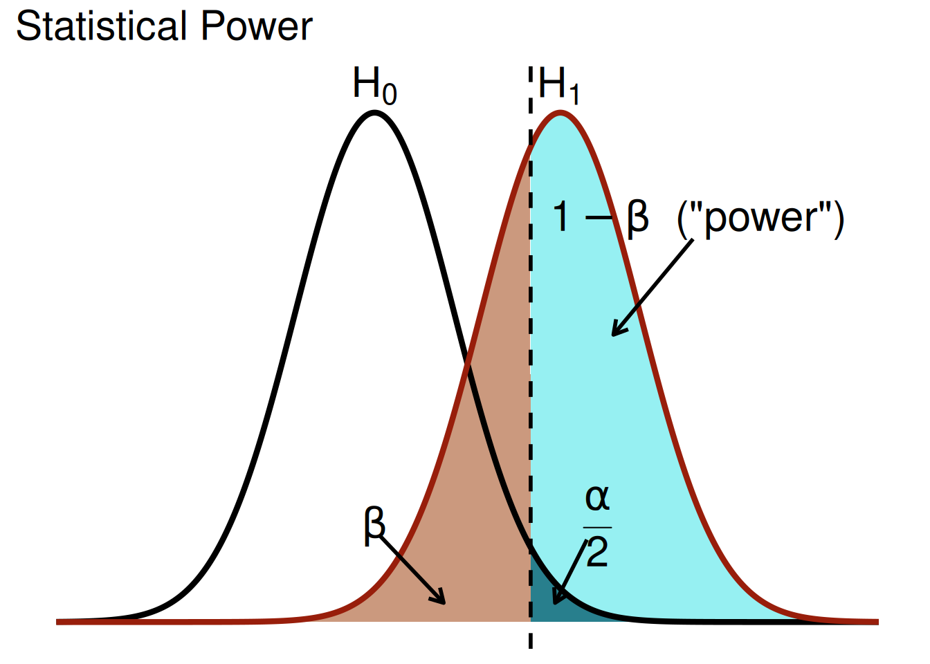
Interactive visualizations by Kristoffer Magnusson on p-values and null-hypothesis significance testing are below:
- https://rpsychologist.com/pvalue (Magnusson, 2021; archived at https://perma.cc/JP9F-9ZVY)
- https://rpsychologist.com/d3/pdist (Magnusson, 2015; archived at https://perma.cc/BE96-8LSJ)
- https://rpsychologist.com/d3/nhst (Magnusson, 2014; archived at https://perma.cc/ZU9A-37F3)
Twelve misconceptions about p-values (Goodman, 2008) are in Table 9.1.
| Number | Misconception |
|---|---|
| 1 | If \(p = .05\), the null hypothesis has only a 5% chance of being true. |
| 2 | A nonsignificant difference (eg, \(p > .05\)) means there is no difference between groups. |
| 3 | A statistically significant finding is clinically important. |
| 4 | Studies with \(p\)-values on opposite sides of .05 are conflicting. |
| 5 | Studies with the same \(p\)-value provide the same evidence against the null hypothesis. |
| 6 | \(p = .05\) means that we have observed data that would occur only 5% of the time under the null hypothesis. |
| 7 | \(p = .05\) and \(p < .05\) mean the same thing. |
| 8 | \(p\)-values are properly written as inequalities (e.g., “\(p \le .05\)” when \(p = .015\)). |
| 9 | \(p = .05\) means that if you reject the null hypothesis, the probability of a Type I error is only 5%. |
| 10 | With a \(p = .05\) threshold for significance, the chance of a Type I error will be 5%. |
| 11 | You should use a one-sided \(p\)-value when you don’t care about a result in one direction, or a difference in that direction is impossible. |
| 12 | A scientific conclusion or treatment policy should be based on whether or not the \(p\)-value is significant. |
That is, the p-value is not:
- the probability that the effect was due to chance
- the probability that the null hypothesis is true
- the size of the effect
- the importance of the effect
- whether the effect is true, real, or causal
Statistical significance involves the consistency of an effect/association/difference; it suggests that the association/difference is reliably non-zero. However, just because something is statistically significant does not mean that it is important. For instance, consider that we discover that players who consume sports drink before a game tend to perform better than players who do not (\(p < .05\)). However, what if consumption of sports drinks is associated with an average improvement of 0.002 points per game. A small effect such as this might be detectable with a large sample size. This effect would be considered to be reliable/consistent because it is statistically significant. However, such an effect is so small that it results in differences that are not practically important. Thus, in addition to statistical significance, it is also important to consider practical significance.
9.4.2 Practical Significance
Practical significance deals with how large or important the effect/association/difference is. It is based on the magnitude of the effect, called the effect size. Effect size can be quantified in various ways including:
- Cohen’s \(d\)
- Standardized regression coefficient (beta; \(\beta\))
- Correlation coefficient (\(r\))
- Cohen’s \(\omega\) (omega)
- Cohen’s \(f\)
- Cohen’s \(f^2\)
- Coefficient of determination (\(R^2\))
- Eta squared (\(\eta^2\))
- Partial eta squared (\(\eta_p^2\))
9.4.2.1 Cohen’s \(d\)
Cohen’s \(d\) is commonly used for evaluating the magnitude of group differences. Cohen’s \(d\) is calculated as in Equation 9.12:
\[ \begin{aligned} d &= \frac{\text{mean difference}}{\text{pooled standard deviation}} \\ &= \frac{\bar{x_1} - \bar{x_2}}{s} \\ \end{aligned} \tag{9.12}\]
where \(\bar{x_1}\) and \(\bar{x_2}\) is the mean for group 1 and group 2, respectively, and:
\[ s = \sqrt{\frac{(n_1 - 1)s_1^2 + (n_2 - 1)s_2^2}{n_1 + n_2 - 2}} \tag{9.13}\]
where \(n_1\) and \(n_2\) is the sample size of group 1 and group 2, respectively, and \(s_1\) and \(s_2\) is the standard deviation of group 1 and group 2, respectively.
Cohen’s \(d\) is interpreted as the mean of group 1 was _ standard deviation units [larger/smaller] than the mean of group 2.
9.4.2.2 Standardized Regression Coefficient (Beta; \(\beta\))
The standardized regression coefficient (beta; \(\beta\)) is used in multiple regression, and is calculated as in Equation 9.14:
\[ \beta_x = B_x \times \frac{s_x}{s_y} \tag{9.14}\]
where \(B_x\) is the unstandardized regression coefficient of the predictor variable \(x\) in predicting the outcome variable \(y\), \(s_x\) is the standard deviation of \(x\), and \(s_y\) is the standard deviation of \(y\). The standardized regression coefficient is interpreted such that, for every 1 standard deviation increase in \(x\), there was a _ standard deviation [increase/decrease] in \(y\).
9.4.2.3 Correlation Coefficient (\(r\))
The formula for the correlation coefficient is in Equation 9.28.
9.4.2.4 Cohen’s \(\omega\)
Cohen’s \(\omega\) is used in chi-square tests, and is calculated as in Equation 9.15:
\[ \omega = \sqrt{\frac{\chi^2}{N} - \frac{df}{N}} \tag{9.15}\]
where \(\chi^2\) is the chi-square statistic from the test, \(N\) is the sample size, and \(df\) is the degrees of freedom.
9.4.2.5 Cohen’s \(f\)
Cohen’s \(f\) is commonly used in ANOVA, and is calculated as in Equation 9.16:
\[ \begin{aligned} f &= \sqrt{\frac{R^2}{1 - R^2}} \\ &= \sqrt{\frac{\eta^2}{1 - \eta^2}} \end{aligned} \tag{9.16}\]
9.4.2.6 Cohen’s \(f^2\)
Cohen’s \(f^2\) is commonly used in regression, and is calculated as in Equation 9.17:
\[ \begin{aligned} f^2 &= \frac{R^2}{1 - R^2} \\ &= \frac{\eta^2}{1 - \eta^2} \end{aligned} \tag{9.17}\]
To calculate the effect size of a particular predictor, you can calculate \(\Delta f^2\) as in Equation 9.18:
\[ \begin{aligned} \Delta f^2 &= \frac{R^2_{\text{model}} - R^2_{\text{reduced}}}{1 - R^2_{\text{model}}} \\ &= \frac{\eta^2_{\text{model}} - \eta^2_{\text{reduced}}}{1 - \eta^2_{\text{model}}} \end{aligned} \tag{9.18}\]
where \(R^2_{\text{model}}\) is the \(R^2\) of the model with the predictor variable of interest and \(R^2_{\text{reduced}}\) is the \(R^2\) of the model without the predictor variable of interest.
9.4.2.7 Coefficient of Determination (\(R^2\))
The coefficient of determination (\(R^2\)) reflects the proportion of variance in the outcome variable that is explained by the predictor variable(s). \(R^2\) is commonly used in regression, and is calculated as in Equation 9.19:
\[ \begin{aligned} R^2 &= 1 - \frac{\sum (y_i - \hat{y}_i)^2}{\sum (y_i - \bar{y})^2} \\ &= 1 - \frac{SS_{\text{residual}}}{SS_{\text{total}}} \\ &= 1 - \frac{\text{sum of squared residuals}}{\text{total sum of squares}} \\ &= \frac{f^2}{1 + f^2} \\ &= \eta^2 \\ &= \frac{\text{variance explained in }y}{\text{total variance in }y} \end{aligned} \tag{9.19}\]
where \(y\) is the outcome variable, \(y_i\) is the observed value of the outcome variable for the \(i\)th observation, \(\hat{y}_i\) is the model predicted value for the \(i\)th observation, and \(\bar{y}\) is the mean of the observed values of the outcome variable. The total sum of squares is an index of the total variation in the outcome variable.
The coefficient of determination typically ranges from 0 to 1, but it can be negative. A negative coefficient of determination indicates that the predicted values are less accurate than using the mean of the actual values as the predicted values (i.e., predicting the mean of the observed values for every case).
9.4.2.8 Squared Semi-Partial Correlation (\(sr^2\))
Squared semi-partial correlations are described in Section 11.7.
9.4.2.9 Eta Squared (\(\eta^2\)) and Partial Eta Squared (\(\eta_p^2\))
Like \(R^2\), eta squared (\(\eta^2\)) reflects the proportion of variance in the dependent variable that is explained by the independent variable(s). \(\eta^2\) is commonly used in ANOVA, and is calculated as in Equation 9.20:
\[ \begin{aligned} \eta^2 &= \frac{SS_{\text{effect}}}{SS_{\text{total}}} \\ &= 1 - \frac{SS_{\text{residual}}}{SS_{\text{total}}} \\ &= 1 - \frac{\text{sum of squared residuals}}{\text{total sum of squares}} \\ &= \frac{f^2}{1 + f^2} \\ &= R^2 \end{aligned} \tag{9.20}\]
where \(SS_{\text{effect}}\) is the sum of squares for the effect of interest and \(SS_{\text{total}}\) is the total sum of squares.
Partial eta squared (\(\eta_p^2\)) reflects the proportion of variance in the dependent variable that is explained by the independent variable while controlling for the other independent variables. \(\eta_p^2\) is commonly used in ANOVA, and is calculated as in Equation 9.21:
\[ \eta_p^2 = \frac{SS_{\text{effect}}}{SS_{\text{effect}} + SS_{\text{error}}} \tag{9.21}\]
where \(SS_{\text{effect}}\) is the sum of squares for the effect of interest and \(SS_{\text{error}}\) is the sum of squares for the residual error term.
9.4.2.10 Effect Size Thresholds
Effect size thresholds (Cohen, 1988; McGrath & Meyer, 2006) for small, medium, and large effect sizes are in Table 9.2.
| Effect Size Index | Small | Medium | Large |
|---|---|---|---|
| Cohen’s \(d\) | \(\ge |.20|\) | \(\ge |.50|\) | \(\ge |.80|\) |
| Standardized regression coefficient (beta; \(\beta\)) | \(\ge |.10|\) | \(\ge |.24|\) | \(\ge |.37|\) |
| Correlation coefficient (\(r\)) | \(\ge |.10|\) | \(\ge |.24|\) | \(\ge |.37|\) |
| Cohen’s \(\omega\) | \(\ge .10\) | \(\ge .30\) | \(\ge .50\) |
| Cohen’s \(f\) | \(\ge .10\) | \(\ge .25\) | \(\ge .40\) |
| Cohen’s \(f^2\) | \(\ge .01\) | \(\ge .06\) | \(\ge .16\) |
| Coefficient of determination (\(R^2\)) | \(\ge .01\) | \(\ge .06\) | \(\ge .14\) |
| Squared semi-partial correlation (\(sr^2\)) | \(\ge .01\) | \(\ge .06\) | \(\ge .14\) |
| Eta squared (\(\eta^2\)) | \(\ge .01\) | \(\ge .06\) | \(\ge .14\) |
| Partial eta squared (\(\eta_p^2\)) | \(\ge .01\) | \(\ge .06\) | \(\ge .14\) |
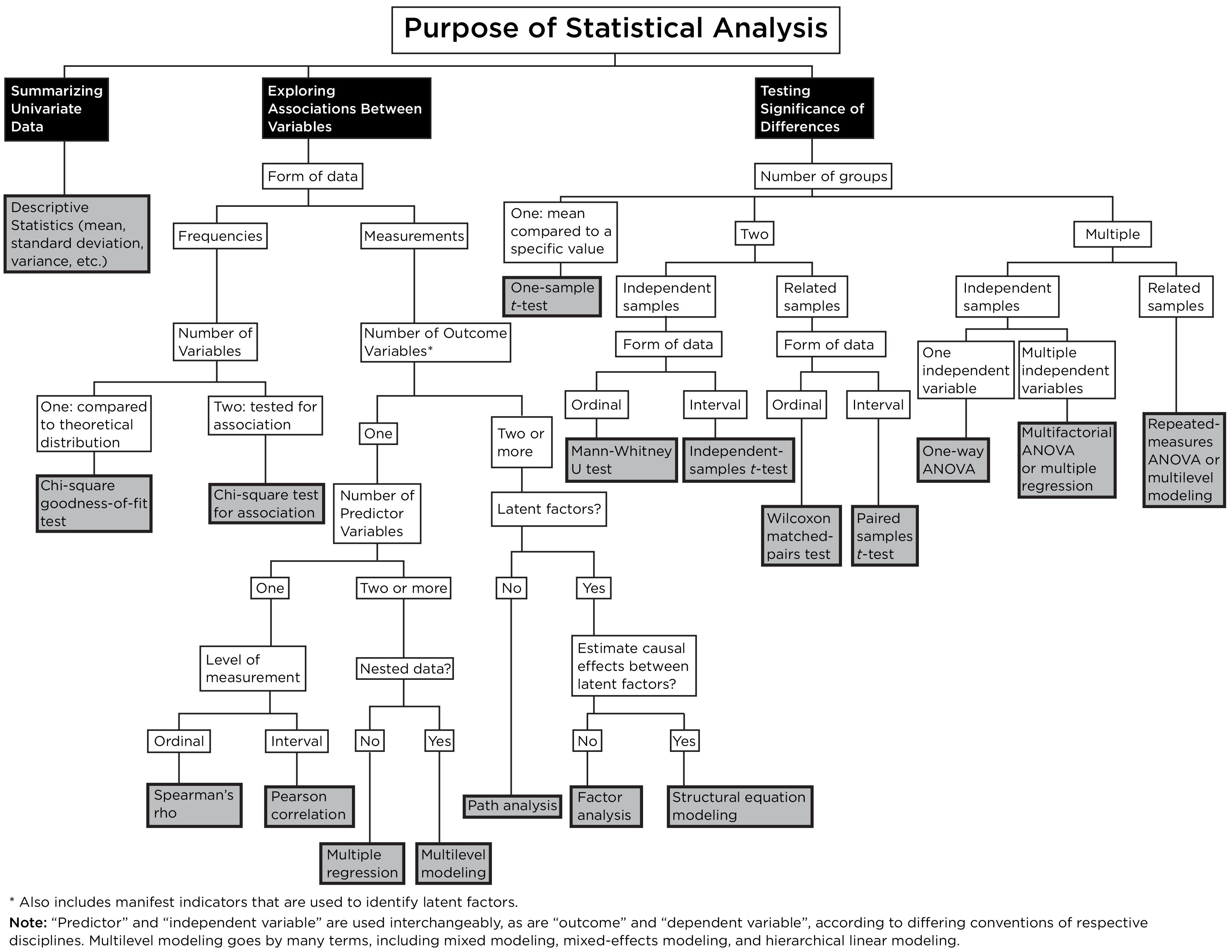
9.5 Statistical Decision Tree
A statistical decision tree is a flowchart or decision tree that depicts which statistical test to use given the purpose of analysis, the type of data, etc. An example statistical decision tree is depicted in Figure 9.8.
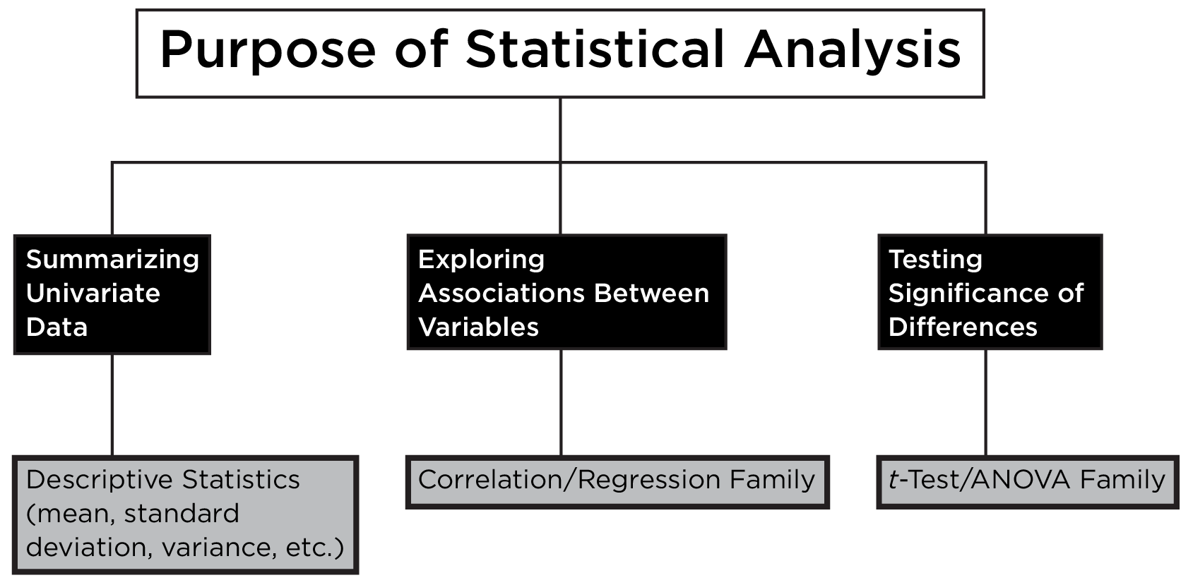
This statistical decision tree can be generally summarized such that associations are examined with the correlation/regression family, and differences are examined with the t-test/ANOVA family, as depicted in Figure 9.9.
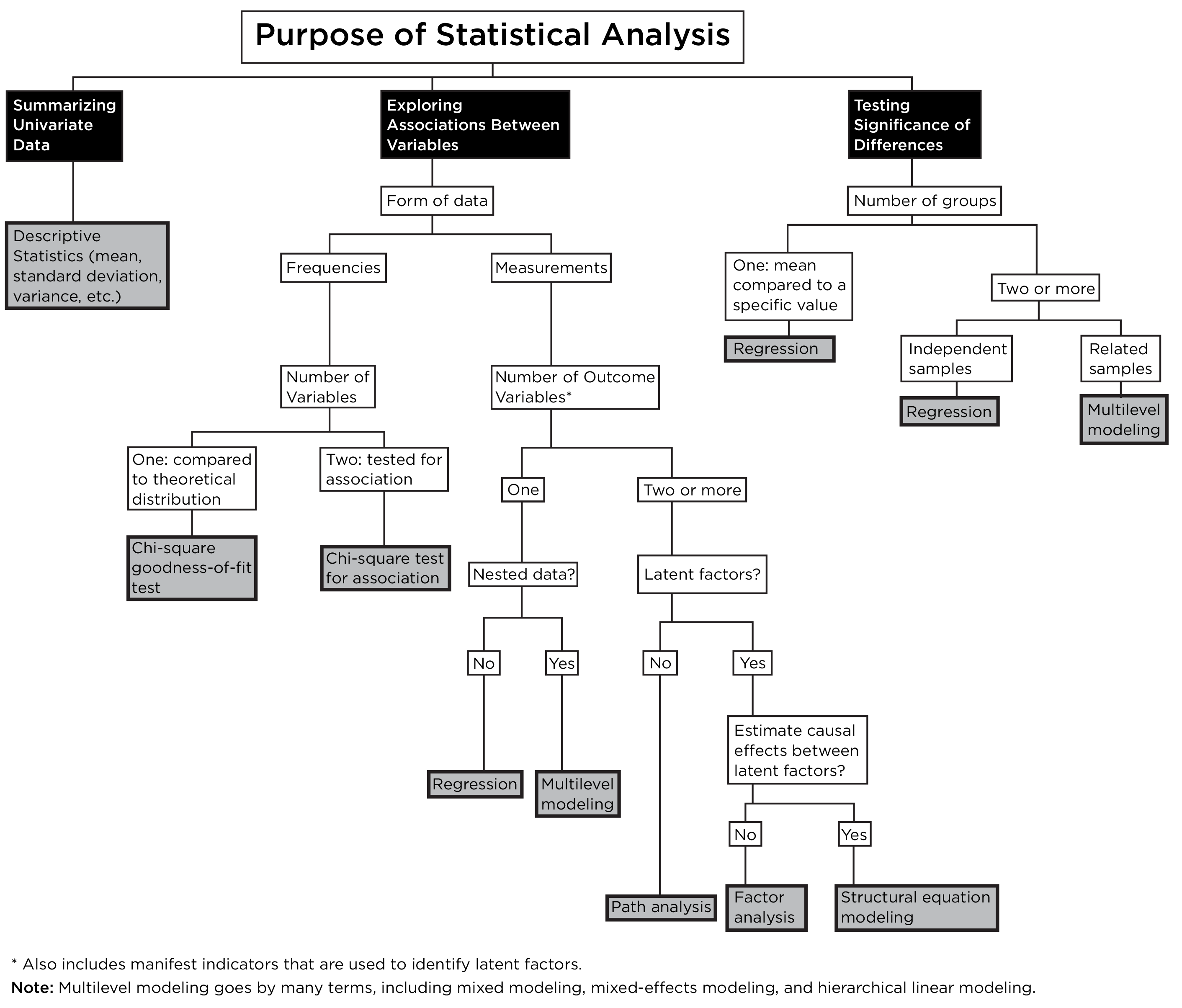
However, many statistical tests can be re-formulated in a regression framework, as in Figure 9.10.
Both associations and differences can be examined with the regression family, which greatly simplifies our summary of the statistical decision tree, as depicted in Figure 9.11.
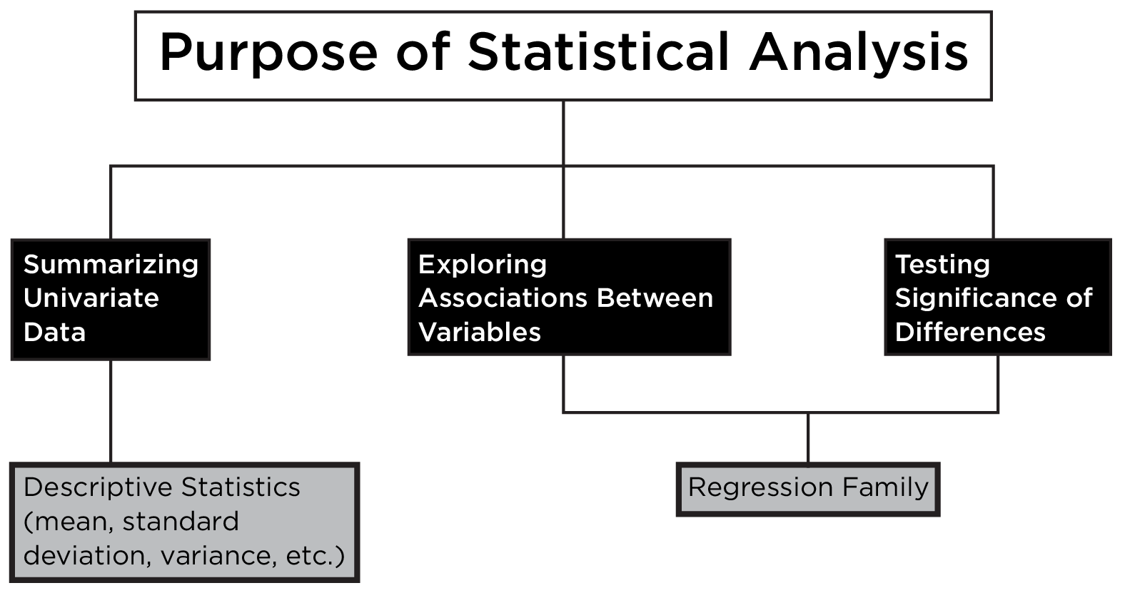
Thus, in most cases, the regression framework can be used to examine most questions regarding associations between variables or differences between groups. Indeed, t-test, ANOVA, and regression are all special cases of the general linear model, which in turn, is a special case of mixed models without random effects (Brauer & Curtin, 2018).
Jackson-Wood (2017) provides an online, interactive statistical decision tree to help you decide which statistical analysis to use: https://www.statsflowchart.co.uk
9.6 Statistical Tests
9.6.1 t-Test
There are several t-tests:
- one-sample t-test
- two-samples t-test
- independent samples t-test
- paired samples t-test
A one-sample t-test is used to evaluate whether a sample mean differs systematically from a particular value. The null hypothesis is that the sample mean does not differ systematically from the pre-specified value. The alternative hypothesis is that the sample mean differs systematically from the pre-specified value. For instance, let’s say you want to test out a new draft strategy. You could participate in a mock draft and draft players using the new strategy. Then, you could use a one-sample t-test to evaluate whether your new draft strategy yields players with more projected points than the average of players’ projected points for other teams.
Two-samples t-tests are used to test for differences between scores of two groups. If the two groups are independent, the independent samples t-test is used. If the two groups involve paired samples, the paired samples t-test is used. The null hypothesis is that the mean of group 1 does not differ systematically from the mean of group 2. The alternative hypothesis is that the mean of group 1 differs systematically from the mean of group 2. For instance, you could use an independent-samples t-test if you want to examine whether Quarterbacks tend to have have longer careers than Running Backs. By contrast, you could use a paired samples t-test if you want to examine whether Quarterbacks tend to score more points in the second year of their contract compared to their rookie year, because the same subjects were assessed twice (i.e., a within-subject design).
9.6.2 Analysis of Variance
Analysis of variance (ANOVA) allows examining whether groups differ systematically as a function of one or more factors. There are multiple variants of ANOVA:
- one-way ANOVA
- factorial ANOVA
- repeated measures ANOVA (RM-ANOVA)
- multivariate ANOVA (MANOVA)
The F statistic (which is used to determine statistical significance) in ANOVA is computed by first partitioning the sum of squares as in Equation 9.22:
\[ SS_{\text{total}} = SS_{\text{between}} + SS_{\text{within}} \tag{9.22}\]
where \(SS_{\text{total}}\) is the total sum of squares, which is equal to Equation 9.23:
\[ SS_{\text{total}} = \sum_{i = 1}^{k} \sum_{j = 1}^{n_i} \left( X_{ij} - \bar{X}_{..} \right)^2 \tag{9.23}\]
where \(X_{ij}\) is the raw data point (i.e., observation \(j\) within group \(i\)), \(n_i\) is the sample size of group \(i\), \(\bar{X}_{i.}\) is the mean of group \(i\), and \(\bar{X}_{..}\) is the grand mean (the mean across all observations from all groups).
\(SS_{\text{between}}\) is the between-groups sum of squares, which is equal to Equation 9.24:
\[ SS_{\text{between}} = \sum_{i = 1}^{k} n_i \left( \bar{X}_{i.} - \bar{X}_{..} \right)^2 \tag{9.24}\]
and \(SS_{\text{within}}\) is the within-groups sum of squares, which is equal to Equation 9.25:
\[ SS_{\text{within}} = \sum_{i = 1}^{k} \sum_{j = 1}^{n_i} \left( X_{ij} - \bar{X}_{i.} \right)^2 \tag{9.25}\]
Mean squares are then computed from the sum of squares as in Equation 9.26:
\[ \begin{aligned} MS_{\text{between}} &= \frac{SS_{\text{between}}}{df_{\text{between}}} &=& \frac{SS_{\text{between}}}{k - 1} \\ MS_{\text{within}} &= \frac{SS_{\text{within}}}{df_{\text{within}}} &=& \frac{SS_{\text{within}}}{N - k} \end{aligned} \tag{9.26}\]
where \(df_{\text{between}}\) is the between-groups degrees of freedom, \(df_{\text{within}}\) is the within-groups degrees of freedom, \(k\) is the number of groups, and \(N\) is the sample size.
Then, the F statistic is computed as the ratio of between-groups mean squares to within-groups mean squares as in Equation 9.27:
\[ F = \frac{MS_{\text{between}}}{MS_{\text{within}}} \tag{9.27}\]
In sum, ANOVA examines the ratio of between-groups sum of squares to within-groups sum of squares (after adjusting for degrees of freedom).
Like two-samples t-tests, ANOVA allows examining whether groups differ as a function of an independent variable. However, unlike a t-test, ANOVA allows examining multiple independent variables and more than two groups. The null hypothesis is that the the groups’ mean value does not differ systematically. The alternative hypothesis is that the groups’ mean value differs systematically.
A one-way ANOVA examines whether two or more groups differ as a function of an independent variable. For instance, you could use a one-way ANOVA to evaluate if you want to evaluate whether multiple positions differ in their length of career. Factorial ANOVA examines whether two or more groups differ as a function of multiple independent variables. For instance, you could use factorial ANOVA to evaluate whether one’s length of career depends on one’s position and weight. Repeated measures ANOVA examines whether scores differ across repeated measures (e.g., across time) for the same participants. For instance, you could use repeated-measures ANOVA to evaluate whether rookies score more points as the season progresses. Multivariate ANOVA examines whether multiple dependent variables differ as a function of one or more factor(s). For instance, you could use MANOVA to evaluate whether one’s contract length and pay differ as a function of one’s position.
ANOVA has key limitations. ANOVA cannot handle continuous independent or predictor variables that vary within units (Brauer & Curtin, 2018). In addition, ANOVA poorly handles missing data—it uses listwise deletion and thus excludes participants with missing values on any of the independent or dependent variables (Brauer & Curtin, 2018).
9.6.3 Correlation
Correlation examines the association between a predictor and outcome variable. The null hypothesis is that the the two variables are not associated. The alternative hypothesis is that the two variables are associated.
The Pearson correlation coefficient (\(r\)) is calculated as in Equation 9.28:
\[ \small \begin{aligned} r &= \frac{\frac{1}{n - 1} \sum_{i=1}^{n} (x_i - \bar{x})(y_i - \bar{y})} {\sqrt{\frac{1}{n - 1} \sum_{i=1}^{n} (x_i - \bar{x})^2} \sqrt{\frac{1}{n - 1} \sum_{i=1}^{n} (y_i - \bar{y})^2}} && \quad \text{the numerator is the covariance; the denominator is the standard deviations} \\ &= \frac{\sum_{i=1}^{n} (x_i - \bar{x})(y_i - \bar{y})} {\sqrt{\sum_{i=1}^{n} (x_i - \bar{x})^2} \sqrt{\sum_{i=1}^{n} (y_i - \bar{y})^2}} && \quad \text{$n-1$ cancels out in numerator and denominator (typical formula for Pearson correlation)} \\ &= \frac{\frac{1}{n - 1} \sum_{i=1}^{n} (x_i - \bar{x})(y_i - \bar{y})}{s_x \cdot s_y} && \quad \text{adding back $n-1$, replacing denominator from line 1 with standard deviation symbols} \\ &= \frac{\text{Cov}(x, y)}{s_x \cdot s_y} && \quad \text{replacing numerator with covariance notation} \\ &= \frac{\sum z_x z_y}{n - 1} \end{aligned} \tag{9.28}\]
where \(x\) is the predictor variable, \(y\) is the outcome variable, \(\text{Cov}(x, y)\) is the covariance between \(x\) and \(y\), \(s_x\) is the standard deviation of \(x\), \(s_y\) is the standard deviation of \(y\), \(n\) is the sample size, \(z_x\) is the z scores for \(x\), and \(z_y\) is the z scores for \(y\).
9.6.4 (Multiple) Regression
Regression, like correlation, examines the association between a predictor and outcome variable. However, unlike correlation, regression allows multiple predictor variables.
Regression with a single predictor takes the form in Equation 11.2. A regression line is depicted in Figure 11.29. Multiple regression (i.e., regression with multiple predictors) takes the form in Equation 11.3.
The null hypothesis is that the the predictor variable(s) are not associated with the outcome variable. The alternative hypothesis is that the predictor variable(s) are associated with the outcome variable.
9.6.5 Chi-Square Test
There are two primary types of chi-square tests:
- chi-square goodness-of-fit test
- chi-square test for association (aka test of independence)
The chi-square goodness-of-fit test evaluates whether a set of categorical data came from a specified distribution. The null hypothesis is that the data came from the specified distribution. The alternative hypothesis is that the data did not come from the specified distribution.
The chi-square test for association evaluates whether two categorical variables are associated. The null hypothesis is that the two variables are not associated. The alternative hypothesis is that the two variables are associated.
9.6.6 Formulating Statistical Tests in Terms of Partitioned Variance
Many statistical tests can be formulated in terms of partitioned variance.
For instance, the t statistic from the independent-samples t-test and the F statistic from ANOVA can be thought of as the ratio of between-group variance to within-group variance, as in Equation 9.29:
\[ t \text{ or } F = \frac{\text{between-group variance}}{\text{within-group variance}} \tag{9.29}\]
The correlation coefficient can be thought of as the ratio of shared variance (i.e., covariance) to total variance, as in Equation 9.30:
\[ r = \frac{\text{shared variance}}{\text{total variance}} \tag{9.30}\]
The coefficient of determination (\(R^2\)) is the proportion of variance in the outcome variable that is explained by the predictor variables. \(\eta^2\) is the proportion of variance in the dependent variable that is explained by the independent variables. The coefficient of determination and \(\eta^2\) can be expressed as the ratio of variance explained in the outcome or dependent variable to the total variance in the outcome or dependent variable, as in Equation 9.31:
\[ R^2 \text{ or } \eta^2 = \frac{\text{variance explained in the outcome variable}}{\text{total variance in the outcome variable}} \tag{9.31}\]
9.6.7 Critical Value
The critical value is the test value for a given test, above which the effect is considered to be statistically significant. The critical value for statistical significance for each test can be determined based on the degrees of freedom and alpha level. The degrees of freedom (df) refer to the number of values in the calculation of a test statistic that are free to vary.
9.6.7.1 One-Sample t-Test
For a one-sample t-test, the degrees of freedom is in Equation 9.32:
\[ df = N - 1 \tag{9.32}\]
where \(N\) is sample size.
One-tailed test (stats::qt()):
Two-tailed test (stats::qt()):
9.6.7.2 Independent-Samples t-Test
For an independent-samples t-test, the degrees of freedom is in Equation 9.33:
\[ df = n_1 + n_2 - 2 \tag{9.33}\]
where \(n_1\) is the sample size of group 1 and \(n_2\) is the sample size of group 2.
One-tailed test (stats::qt()):
Two-tailed test (stats::qt()):
9.6.7.3 Paired-Samples t-Test
For a paired-samples t-test, the degrees of freedom is in Equation 9.34:
\[ df = N - 1 \tag{9.34}\]
where \(N\) is sample size (i.e., the number of paired observations).
One-tailed test (stats::qt()):
Two-tailed test (stats::qt()):
9.6.7.4 One-Way ANOVA
For a one-way ANOVA, the degrees of freedom is in Equation 9.35:
\[ \begin{aligned} df_\text{between} &= g - 1 \\ df_\text{within} &= N - g \end{aligned} \tag{9.35}\]
where \(N\) is sample size and \(g\) is the number of groups.
One-tailed test (stats::qf()):
Two-tailed test (stats::qf()):
9.6.7.5 Factorial ANOVA
For a factorial two-way ANOVA, the degrees of freedom is in Equation 9.36:
\[ \begin{aligned} df_\text{Factor A} &= a - 1 \\ df_\text{Factor B} &= b - 1 \\ df_\text{Interaction} &= (a - 1)(b - 1) \\ df_\text{error} &= ab(N - 1) \end{aligned} \tag{9.36}\]
where \(N\) is sample size, \(a\) is the number of levels for factor A, and \(b\) is the number of levels for factor B.
Factor A (one-tailed test; stats::qf()):
Factor B (one-tailed test; stats::qf()):
Interaction (one-tailed test; stats::qf()):
Factor A (two-tailed test; stats::qf()):
Factor B (two-tailed test; stats::qf()):
Interaction (two-tailed test; stats::qf()):
9.6.7.6 Repeated Measures ANOVA
For a repeated measures ANOVA, the degrees of freedom is in Equation 9.37:
\[ \begin{aligned} df_1 &= T - 1 \\ df_2 &= (T - 1)(N - 1) \end{aligned} \tag{9.37}\]
where \(N\) is sample size and \(T\) is the number of measurements (i.e., the number of levels of the within-person factor: e.g., timepoints or conditions).
One-tailed test (stats::qf()):
Two-tailed test (stats::qf()):
9.6.7.7 Correlation
For a correlation, the degrees of freedom is in Equation 9.38:
\[ df = N - 2 \tag{9.38}\]
where \(N\) is sample size.
One-tailed test (stats::qt()):
Two-tailed test (stats::qt()):
9.6.7.8 Multiple Regression
For multiple regression, the degrees of freedom is in Equation 9.39:
\[ \begin{aligned} df_1 &= p \\ df_2 &= N - p - 1 \end{aligned} \tag{9.39}\]
where \(N\) is sample size and \(p\) is the number of predictors.
One-tailed test (stats::qf()):
Two-tailed test (stats::qf()):
9.6.7.9 Chi-Square Goodness-of-Fit Test
For the chi-square goodness-of-fit test, the degrees of freedom is in Equation 9.40:
\[ df = c - 1 \tag{9.40}\]
where \(c\) is the number of categories.
One-tailed test (stats::qchisq()):
Two-tailed test (stats::qchisq()):
9.6.7.10 Chi-Square Test for Association
For the chi-square test for association, the degrees of freedom is in Equation 9.41:
\[ df = (r - 1) \times (c - 1) \tag{9.41}\]
where \(r\) is the number of rows in the contingency table and \(c\) is the number of columns in the contingency table.
One-tailed test (stats::qchisq()):
Two-tailed test (stats::qchisq()):
9.6.8 Statistical Power
As described above, statistical power is the probability of detecting an effect, if, in fact, the effect exists. Statistical power for a given test can be calculated based on three factors:
- effect size
- sample size
- alpha level (Type I error rate)
Knowing any three of the following, you can calculate the fourth (assuming the assumptions of the statistical test are met): statistical power, effect size, sample size, and alpha level (Type I error rate). Below is R code for calculating power for each of various statistical tests (i.e., a power analysis). We use the pwr (Champely, 2020) and pwrss (Bulus, 2023) packages to estimate statistical power. For free point-and-click software for calculating statistical power, see G*Power: https://www.psychologie.hhu.de/arbeitsgruppen/allgemeine-psychologie-und-arbeitspsychologie/gpower.html
When designing a study, it is important to consider power and the sample size needed to detect the hypothesized effect size. If your sample size is too small and you do not detect an effect (i.e., \(p > .05\)), you do not know whether your failure to detect the effect was because a) the effect does not exist, or b) the effect exists but you did not have enough power to detect it.
9.6.8.1 One-Sample t-Test
Solving for statistical power achieved (given effect size, sample size, and alpha level; pwr::pwr.t.test()):
Code
     One-sample t test power calculation

              n = 200
              d = 0.5
      sig.level = 0.05
          power = 0.9999998
    alternative = two.sided
Solving for sample size needed (given effect size, power, and alpha level):
Code
     One-sample t test power calculation

              n = 33.36713
              d = 0.5
      sig.level = 0.05
          power = 0.8
    alternative = two.sided
Solving for the minimum detectable effect size (given sample size, power, and alpha level):
9.6.8.2 Independent-Samples t-Test
9.6.8.2.1 Balanced Group Sizes
Solving for statistical power achieved (given effect size, sample size per group, and alpha level; pwr::pwr.t.test()):
Code
     Two-sample t test power calculation

              n = 200
              d = 0.5
      sig.level = 0.05
          power = 0.9987689
    alternative = two.sided

NOTE: n is number in *each* group
Solving for sample size per group needed (given effect size, power, and alpha level):
Code
     Two-sample t test power calculation

              n = 63.76561
              d = 0.5
      sig.level = 0.05
          power = 0.8
    alternative = two.sided

NOTE: n is number in *each* group
Solving for the minimum detectable effect size (given sample size per group, power, and alpha level):
9.6.8.2.2 Unbalanced Group Sizes
Solving for statistical power achieved (given effect size, sample size per group, and alpha level; pwr::pwr.t2n.test()):
Code
     t test power calculation

             n1 = 150
             n2 = 150
              d = 0.5
      sig.level = 0.05
          power = 0.9907677
    alternative = two.sided
Solving for sample size per group needed (given effect size, power, and alpha level):
Code
     t test power calculation

             n1 = 150
             n2 = 40.22483
              d = 0.5
      sig.level = 0.05
          power = 0.8
    alternative = two.sided
Solving for the minimum detectable effect size (given sample size per group, power, and alpha level):
9.6.8.3 Paired-Samples t-Test
Solving for statistical power achieved (given effect size, sample size per group, and alpha level; pwr::pwr.t.test()):
Code
     Paired t test power calculation

              n = 200
              d = 0.5
      sig.level = 0.05
          power = 0.9999998
    alternative = two.sided

NOTE: n is number of *pairs*
Solving for sample size per group needed (given effect size, power, and alpha level):
Code
     Paired t test power calculation

              n = 33.36713
              d = 0.5
      sig.level = 0.05
          power = 0.8
    alternative = two.sided

NOTE: n is number of *pairs*
Solving for the minimum detectable effect size (given sample size per group, power, and alpha level):
9.6.8.4 One-Way ANOVA
Solving for statistical power achieved (given effect size, sample size per group, and alpha level; pwr::pwr.anova.test()):
     Balanced one-way analysis of variance power calculation

              k = 4
              n = 200
              f = 0.25
      sig.level = 0.05
          power = 0.9999962

NOTE: n is number in each group
Solving for sample size per group needed (given effect size, power, and alpha level; pwr::pwr.anova.test()):
     Balanced one-way analysis of variance power calculation

              k = 4
              n = 44.59927
              f = 0.25
      sig.level = 0.05
          power = 0.8

NOTE: n is number in each group
Solving for the minimum detectable effect size (given sample size per group, power, and alpha level; pwr::pwr.anova.test()):
     Balanced one-way analysis of variance power calculation

              k = 4
              n = 200
              f = 0.117038
      sig.level = 0.05
          power = 0.8

NOTE: n is number in each group
9.6.8.4.1 Simulation
The power analysis code above assumes the groups are of equal size (i.e., a balanced design). If the design is unbalanced (i.e., there are different numbers of participants in each group), it may be necessary to conduct a power analysis via a simulation. Below is an example of evaluating the statistical power for detecting an effect unbalanced designs via simulation using the SimDesign (Chalmers, 2025; Chalmers & Adkins, 2020) package. We discuss simulation more in Chapter 24.
9.6.8.4.1.1 1. Design Matrix
First, we set up the design matrix using the SimDesign::createDesign() function:
9.6.8.4.1.2 2. Generate
Second, we set up the Generate() function:
Code
Generate <- function(condition, fixed_objects = NULL) {
  with(condition, {
    # Means for each group
    mean1 <- 0
    mean2 <- f * sqrt((nGroup1 + nGroup2) / 2)

    # Generate data
    group1 <- rnorm(nGroup1, mean = mean1, sd = 1)
    group2 <- rnorm(nGroup2, mean = mean2, sd = 1)

    data.frame(
      value = c(group1, group2),
      group = factor(rep(c("Group1", "Group2"),
                         c(nGroup1, nGroup2)))
    )
  })
}
9.6.8.4.1.3 3. Analyse
Third, we set up the Analyse() function:
9.6.8.4.1.4 4. Summarise
Fourth, we set up the Summarise() function:
9.6.8.4.1.5 5. Run the Simulation
Fifth, we run the simulation using the SimDesign::runSimulation() function:
9.6.8.4.1.6 Simulation Results
Here are the simulation results:
9.6.8.5 Factorial ANOVA
The power analysis code below assumes the groups are of equal size (i.e., a balanced design). If the design is unbalanced (i.e., there are different numbers of participants in each group), it may be necessary to conduct a power analysis via a simulation. See Section 9.6.8.4 for an example power analysis simulation for one-way ANOVA.
Solving for statistical power achieved (given effect size, sample size per group, and alpha level; pwr::pwr.anova.test()):
     Balanced one-way analysis of variance power calculation

              k = 3
              n = 200
              f = 0.25
      sig.level = 0.05
          power = 0.9999238

NOTE: n is number in each group
     Balanced one-way analysis of variance power calculation

              k = 4
              n = 200
              f = 0.25
      sig.level = 0.05
          power = 0.9999962

NOTE: n is number in each group
Code
     Balanced one-way analysis of variance power calculation

              k = 7
              n = 200
              f = 0.25
      sig.level = 0.05
          power = 1

NOTE: n is number in each group
Solving for sample size per group needed (given effect size, power, and alpha level):
     Balanced one-way analysis of variance power calculation

              k = 3
              n = 52.3966
              f = 0.25
      sig.level = 0.05
          power = 0.8

NOTE: n is number in each group
     Balanced one-way analysis of variance power calculation

              k = 4
              n = 44.59927
              f = 0.25
      sig.level = 0.05
          power = 0.8

NOTE: n is number in each group
Code
     Balanced one-way analysis of variance power calculation

              k = 7
              n = 32.05196
              f = 0.25
      sig.level = 0.05
          power = 0.8

NOTE: n is number in each group
Solving for the minimum detectable effect size (given sample size per group, power, and alpha level):
     Balanced one-way analysis of variance power calculation

              k = 3
              n = 200
              f = 0.1270373
      sig.level = 0.05
          power = 0.8

NOTE: n is number in each group
     Balanced one-way analysis of variance power calculation

              k = 4
              n = 200
              f = 0.117038
      sig.level = 0.05
          power = 0.8

NOTE: n is number in each group
Code
     Balanced one-way analysis of variance power calculation

              k = 7
              n = 200
              f = 0.09889082
      sig.level = 0.05
          power = 0.8

NOTE: n is number in each group
9.6.8.6 Repeated Measures ANOVA
Solving for statistical power achieved (given effect size, sample size per group, and alpha level; WebPower::wp.rmanova()):
Code
Repeated-measures ANOVA analysis

      n    f ng nm nscor alpha     power
    200 0.25  4  4     1  0.05 0.8484718

NOTE: Power analysis for between-effect test
URL: http://psychstat.org/rmanova
Code
Repeated-measures ANOVA analysis

      n    f ng nm nscor alpha     power
    200 0.25  4  4     1  0.05 0.8536292

NOTE: Power analysis for within-effect test
URL: http://psychstat.org/rmanova
Code
Repeated-measures ANOVA analysis

      n    f ng nm nscor alpha     power
    200 0.25  4  4     1  0.05 0.6756298

NOTE: Power analysis for interaction-effect test
URL: http://psychstat.org/rmanova
Solving for sample size per group needed (given effect size, power, and alpha level):
Code
Repeated-measures ANOVA analysis

           n    f ng nm nscor alpha power
    178.3971 0.25  4  4     1  0.05   0.8

NOTE: Power analysis for between-effect test
URL: http://psychstat.org/rmanova
Code
Repeated-measures ANOVA analysis

           n    f ng nm nscor alpha power
    175.7692 0.25  4  4     1  0.05   0.8

NOTE: Power analysis for within-effect test
URL: http://psychstat.org/rmanova
Code
Repeated-measures ANOVA analysis

           n    f ng nm nscor alpha power
    253.2369 0.25  4  4     1  0.05   0.8

NOTE: Power analysis for interaction-effect test
URL: http://psychstat.org/rmanova
Solving for the minimum detectable effect size (given sample size per group, power, and alpha level):
Code
Repeated-measures ANOVA analysis

      n         f ng nm nscor alpha power
    200 0.2358259  4  4     1  0.05   0.8

NOTE: Power analysis for between-effect test
URL: http://psychstat.org/rmanova
Code
Repeated-measures ANOVA analysis

      n         f ng nm nscor alpha power
    200 0.2342726  4  4     1  0.05   0.8

NOTE: Power analysis for within-effect test
URL: http://psychstat.org/rmanova
Code
Repeated-measures ANOVA analysis

      n         f ng nm nscor alpha power
    200 0.2817486  4  4     1  0.05   0.8

NOTE: Power analysis for interaction-effect test
URL: http://psychstat.org/rmanova
9.6.8.7 Correlation
Solving for statistical power achieved (given effect size, sample size per group, and alpha level; pwr::pwr.r.test()):
     approximate correlation power calculation (arctangh transformation)

              n = 200
              r = 0.24
      sig.level = 0.05
          power = 0.9310138
    alternative = two.sided
Solving for sample size per group needed (given effect size, power, and alpha level):
     approximate correlation power calculation (arctangh transformation)

              n = 133.1299
              r = 0.24
      sig.level = 0.05
          power = 0.8
    alternative = two.sided
Solving for the minimum detectable effect size (given sample size per group, power, and alpha level):
9.6.8.8 Multiple Regression
Solving for statistical power achieved (given effect size, sample size, and alpha level; pwr::pwr.f2.test()):
Code
     Multiple regression power calculation

              u = 5
              v = 194
             f2 = 0.06
      sig.level = 0.05
          power = 0.7548031
Code
+--------------------------------------------------+
|                POWER CALCULATION                 |
+--------------------------------------------------+

Linear Regression Coefficient (T-Test)

----------------------------------------------------
Hypotheses
----------------------------------------------------
  H0 (Null)        : beta - null.beta  = 0
  H1 (Alternative) : beta - null.beta != 0

----------------------------------------------------
Results
----------------------------------------------------
  Target Effect (Std. beta) = 0.240
  Sample Size               = 200
  Type 1 Error (alpha)      = 0.050
  Type 2 Error (beta)       = 0.064
  Statistical Power         = 0.936  <<
Solving for sample size needed (given effect size, power, and alpha level)—\(v = N - \text{numberOfPredictors} - 1\); thus, \(N = v + \text{numberOfPredictors} + 1\):
Code
     Multiple regression power calculation

              u = 5
              v = 213.3947
             f2 = 0.06
      sig.level = 0.05
          power = 0.8
Code
[1] 219.3947Code
+--------------------------------------------------+
|             SAMPLE SIZE CALCULATION              |
+--------------------------------------------------+

Linear Regression Coefficient (T-Test)

----------------------------------------------------
Hypotheses
----------------------------------------------------
  H0 (Null)        : beta - null.beta  = 0
  H1 (Alternative) : beta - null.beta != 0

----------------------------------------------------
Results
----------------------------------------------------
  Target Effect (Std. beta) = 0.240
  Sample Size               = 131  <<
  Type 1 Error (alpha)      = 0.050
  Type 2 Error (beta)       = 0.198
  Statistical Power         = 0.802
Solving for the minimum detectable effect size (given sample size, power, and alpha level):
9.6.8.9 Chi-Square Goodness-of-Fit Test
Solving for statistical power achieved (given effect size, sample size, and alpha level; pwr::pwr.chisq.test()):
     Chi squared power calculation

              w = 0.3
              N = 200
             df = 5
      sig.level = 0.05
          power = 0.9269225

NOTE: N is the number of observations
Solving for sample size needed (given effect size, power, and alpha level):
Code
     Chi squared power calculation

              w = 0.3
              N = 142.529
             df = 5
      sig.level = 0.05
          power = 0.8

NOTE: N is the number of observations
Solving for the minimum detectable effect size (given sample size, power, and alpha level):
9.6.8.10 Chi-Square Test for Association
Solving for statistical power achieved (given effect size, sample size, and alpha level; pwr::pwr.chisq.test()):
Code
     Chi squared power calculation

              w = 0.3
              N = 200
             df = 4
      sig.level = 0.05
          power = 0.9431195

NOTE: N is the number of observations
Solving for sample size needed (given effect size, power, and alpha level):
Code
     Chi squared power calculation

              w = 0.3
              N = 132.6143
             df = 4
      sig.level = 0.05
          power = 0.8

NOTE: N is the number of observations
Solving for the minimum detectable effect size (given sample size, power, and alpha level):
9.6.8.11 Multilevel Modeling
Power analysis for multilevel modeling approaches is more complicated than it is for other statistical analyses, such as correlation, multiple regression, t-tests, ANOVA, etc.
There are free web applications for calculating power in multilevel modeling:
9.6.8.12 Path Analysis, Factor Analysis, and Structural Equation Modeling
Power analysis for latent variable modeling approaches like structural equation modeling (SEM) is more complicated than it is for other statistical analyses, such as correlation, multiple regression, t-tests, ANOVA, etc.
I provide an example of power analysis in SEM using Monte Carlo simulation in R here: https://isaactpetersen.github.io/Principles-Psychological-Assessment/sem.html#monteCarloPowerAnalysis (Petersen, 2025b).
There are also free web applications for calculating power in SEM:
9.6.8.13 Mediation and Moderation
There are free tools for calculating power for tests of mediation and moderation:
- https://schoemanna.shinyapps.io/mc_power_med (Schoemann et al., 2017)
-
https://www.causalevaluation.org/power-analysis.html (web application: https://powerupr.shinyapps.io/index/) (Ataneka et al., 2023), based on the
PowerUpRpackage (Bulus et al., 2021) - https://webpower.psychstat.org/wiki/models/index (Zhang & Yuan, 2018)
9.7 Ethics of Reporting Statistics
It is important to report statistics ethically and responsibly. People can use statistics to lie (Huff, 2023). It is important to present statistics fairly and accurately even if they are not convenient to your preferred narrative. In addition, it is important to consider practical significance in addition to statistical significance.
9.8 Conclusion
Descriptive statistics are used to describe the data, including the center, spread, or shape of data. Inferential statistics are used to draw inferences regarding differences between groups or associations between variables. Null hypothesis signficance testing is a framework for inferential statistics, in which there is a null hypothesis and alternative hypothesis. The null hypothesis is that there is no difference between groups or that there is no association between variables. Statistical significance is evaluated with a \(p\)-value, which represents the probability of obtaining a result at least as extreme as the result observed if the null hypothesis is true. Effects with p-values less than .05 are considered statistically significant. However, it is also important to consider practical significance and effect sizes. When designing a study, it is important to consider statistical power and the sample size needed to detect the hypothesized effect size. You can determine a study’s power based on the effect size, sample size, and alpha level.
9.9 Session Info
R version 4.6.1 (2026-06-24)
Platform: x86_64-pc-linux-gnu
Running under: Ubuntu 24.04.4 LTS

Matrix products: default
BLAS:   /usr/lib/x86_64-linux-gnu/openblas-pthread/libblas.so.3
LAPACK: /usr/lib/x86_64-linux-gnu/openblas-pthread/libopenblasp-r0.3.26.so;  LAPACK version 3.12.0

locale:
 [1] LC_CTYPE=C.UTF-8       LC_NUMERIC=C           LC_TIME=C.UTF-8
 [4] LC_COLLATE=C.UTF-8     LC_MONETARY=C.UTF-8    LC_MESSAGES=C.UTF-8
 [7] LC_PAPER=C.UTF-8       LC_NAME=C              LC_ADDRESS=C
[10] LC_TELEPHONE=C         LC_MEASUREMENT=C.UTF-8 LC_IDENTIFICATION=C

time zone: UTC
tzcode source: system (glibc)

attached base packages:
[1] grid      parallel  stats     graphics  grDevices utils     datasets
[8] methods   base

other attached packages:
 [1] lubridate_1.9.5   forcats_1.0.1     stringr_1.6.0     dplyr_1.2.1
 [5] purrr_1.2.2       readr_2.2.0       tidyr_1.3.2       tibble_3.3.1
 [9] ggplot2_4.0.3     tidyverse_2.0.0   SimDesign_2.25    psych_2.6.5
[13] WebPower_0.9.4    PearsonDS_1.3.2   lavaan_0.6-21     lme4_2.0-1
[17] Matrix_1.7-5      MASS_7.3-65       pwrss_1.2.0       pwr_1.3-0
[21] DescTools_0.99.60 petersenlab_1.2.3

loaded via a namespace (and not attached):
  [1] RColorBrewer_1.1-3    rstudioapi_0.19.0     audio_0.1-12
  [4] jsonlite_2.0.0        magrittr_2.0.5        farver_2.1.2
  [7] nloptr_2.2.1          rmarkdown_2.31        fs_2.1.0
 [10] vctrs_0.7.3           minqa_1.2.8           base64enc_0.1-6
 [13] htmltools_0.5.9       haven_2.5.5           cellranger_1.1.0
 [16] Formula_1.2-5         parallelly_1.48.0     htmlwidgets_1.6.4
 [19] plyr_1.8.9            testthat_3.3.2        rootSolve_1.8.2.4
 [22] lifecycle_1.0.5       pkgconfig_2.0.3       R6_2.6.1
 [25] fastmap_1.2.0         rbibutils_2.4.1       future_1.70.0
 [28] digest_0.6.39         Exact_3.3             colorspace_2.1-3
 [31] Hmisc_5.2-6           labeling_0.4.3        progressr_1.0.0
 [34] timechange_0.4.0      mgcv_1.9-4            httr_1.4.8
 [37] compiler_4.6.1        proxy_0.4-29          withr_3.0.3
 [40] htmlTable_2.5.0       S7_0.2.2              backports_1.5.1
 [43] DBI_1.3.0             R.utils_2.13.0        sessioninfo_1.2.4
 [46] gld_2.6.8             tools_4.6.1           pbivnorm_0.6.0
 [49] foreign_0.8-91        otel_0.2.0            future.apply_1.20.2
 [52] clipr_0.8.1           nnet_7.3-20           R.oo_1.27.1
 [55] glue_1.8.1            quadprog_1.5-8        nlme_3.1-169
 [58] checkmate_2.3.4       cluster_2.1.8.2       reshape2_1.4.5
 [61] generics_0.1.4        gtable_0.3.6          tzdb_0.5.0
 [64] R.methodsS3_1.8.2     class_7.3-23          data.table_1.18.4
 [67] lmom_3.3              hms_1.1.4             stringfish_0.19.0
 [70] pillar_1.11.1         mitools_2.4           splines_4.6.1
 [73] lattice_0.22-9        tidyselect_1.2.1      pbapply_1.7-4
 [76] mix_1.0-13            knitr_1.51            reformulas_0.4.4
 [79] gridExtra_2.3.1       stats4_4.6.1          xfun_0.60
 [82] expm_1.0-0            brio_1.1.5            stringi_1.8.7
 [85] yaml_2.3.12           boot_1.3-32           evaluate_1.0.5
 [88] codetools_0.2-20      beepr_2.0             cli_3.6.6
 [91] RcppParallel_5.1.11-2 rpart_4.1.27          xtable_1.8-8
 [94] Rdpack_2.6.6          mirai_2.7.1           Rcpp_1.1.2
 [97] readxl_1.5.0          globals_0.19.1        nanonext_1.10.1
[100] listenv_1.0.0         viridisLite_0.4.3     mvtnorm_1.4-2
[103] scales_1.4.0          e1071_1.7-17          rlang_1.3.0
[106] qs2_0.2.2             mnormt_2.1.2